Villain action in lattice gauge theory

Abstract

We prove that Villain interaction applied to lattice gauge theory can be obtained as the limit of both Wilson and Manton interactions on a larger graph which we call the carpet graph. This is the lattice gauge theory analog of a well-known property for spin $O(N)$ models where Villain type interactions are the limit of $\mathbb{S}^{N-1}$ spin systems defined on a cable graph.

Perhaps surprisingly in the setting of lattice gauge theory, our proof also applies to non-Abelian lattice theory such as $SU(3)$-lattice gauge theory and its limiting Villain interaction.

In the particular case of an Abelian lattice gauge theory, this allows us to extend the validity of Ginibre inequality to the case of the Villain interaction.

1 Introduction

1.1 Context

Our main result (Theorem 1.5 below) states that the Villain action in lattice gauge theory, for any compact connected structure group $G$, is the limit of any other action on so-called carpet graphs that we introduce, provided this action satisfies reasonable assumptions. See Figure 1 for an illustration of the carpet graph and Section 2 for the precise assumptions on the class of actions we consider. Standard actions such as Wilson and Manton (and trivially Villain) satisfy our assumptions.

This result can be seen as analogous to the fact that the 2D Villain model is the 1D scaling limit of the $XY$ model, see [AHPS21, Appendix A].

The Villain action has played a prominent role in the study of spin-$O(N)$ models on $\mathbb{Z}^{d}$ since the 70’s. For example the derivation by Berezinskii of the Berezinskii-Kosterlitz-Thouless phase transition relied on the special duality properties of the Villain interaction (see [berezinskii1971destruction, jose1977renormalization]). See also the recent works [AHPS21, lammers2023bijecting, garban2023quantitative] as well as [dubedat2022random] for a random-cluster perspective on the Villain spin model.

The importance of Villain interaction in $O(N)$ spin systems is two-fold: $i)$ first it provides a natural extension of these spin-systems to the so-called cable graph allowing for a more powerful use of Markov’s property (this idea was popularized in the context of the Gaussian free field on $\mathbb{Z}^{d}$ by Lupu in [lupu2016loop]). And $ii)$, when the spins are $\mathbb{S}^{1}$-valued, the duality with integer-valued height functions is particularly elegant as it involves discrete Gaussians.

This paper focuses instead on lattice gauge theory where the basic randomness is now sampled along (oriented) edges. We refer the reader to [seiler1982gauge, frohlich1982massless, chatterjee2019yang, chatterjee2020wilson, garban2023improved, forsstrom2023wilson, cao2023random] and references therein for background on lattice gauge theory. It turns out that the Villain interaction has also long been considered in this setting of lattice gauge theory, for example in the work of Migdal [Migdal75] on the integrability of 2D quantum Yang–Mills theory (see also [Driver89, Witten91, Levy03]) as well as in the seminal work [frohlich1982massless]. It also plays a key role in the proof of confinement at all temperatures in the breakthrough work by Göpfert-Mack [gopfert1982proof] where Villain lattice gauge theory on $\mathbb{Z}^{3}$ is in duality with the integer-valued Gaussian free field $\Psi\colon\mathbb{Z}^{3}\to\mathbb{Z}$. This duality between Villain lattice gauge theory and $\mathbb{Z}$-valued $k$-forms is also used in [garban2023improved]. The Villain action was also recently used in [CC22] in the study of ultraviolet stability of the Abelian lattice Higgs model.

As far as we know, the fact that such a Villain interaction appears as the limit of a Wilson lattice gauge theory along a “cable-type” graph has not been made explicit in the literature. This is the purpose of this paper where the limit goes through a plaquette version of the cable-graph which we call the carpet graph. See Figure 1. As we shall see below and perhaps somewhat surprisingly, such an extension is also valid for non-Abelian lattice gauge theories.

In the special case of Abelian symmetry, one consequence of this work is the validity of Ginibre correlation inequality for lattice gauge theory with Villain interaction which is obtained through a limiting procedure as in [AHPS21, Appendix A]. See Corollary 1.6 below. It is unclear to us how to deduce such a correlation inequality without going through the carpet graph limit, see Remark 1.7.

This paper is self-contained modulo several analytic results that we reference.

1.2 Preliminaries

Let $\Lambda^{d}=\{x\in\mathbb{Z}^{d}\,:\,|x|_{\infty}\leq L\}$ be a box in $\mathbb{Z}^{d}$ with side length $2L$, where $|x|_{\infty}=\mathop{\mathrm{max}}_{i=1,\ldots,d}|x_{i}|$. Let $e_{1},\ldots,e_{d}$ be the canonical basis of $\mathbb{R}^{d}$. Let E = {(x,e_j)  :  x∈Λ^d, x+e_j ∈Λ^d, 1≤j≤d} denote the positively oriented edges that are contained in $\Lambda^{d}$. Let P={(x,e_i,e_j) :  x,x+e_i,x+e_j∈Λ, 1≤i¡j≤d} denote the set of plaquettes of $\Lambda^{d}$.

Let $G$ be a compact matrix group with a Haar measure $\mathop{}\!\mathrm{d}x$. Consider a function $Q\colon G\to[0,\infty)$ such that $Q(xyx^{-1})=Q(y)$ and $Q(x)=Q(x^{-1})$ and $\int_{G}Q(x)\mathop{}\!\mathrm{d}x=1$ (one should think that $Q=e^{-S}$ for an action $S$ on $G$). Define the probability measure $\mu_{Q}$ on $G^{E}$ by [eq:LGT] μ_Q(​dU) = Z_Q^-1 ∏_p∈PQ(U_p) ​dU where $Z_{Q}$ is a normalisation constant and where U_p =defU_(x,e_i)U_(x+e_i,e_j)U_(x+e_j,e_i)^-1U_(x,e_j)^-1 is the holonomy of $U$ around $p=(x,e_{i},e_{j})\in P$, and $\mathop{}\!\mathrm{d}U$ is the Haar measure on $G^{E}$.

1.3 Main result

Definition 1.1 (Carpet graph)

For $N\geq 1$, let $\Lambda^{d}_{N}$ denote the lattice $\Lambda^{d}$ where we tile every plaquette $p\in P$ with $N^{2}$ plaquettes of size $\varepsilon\times\varepsilon$ where $\varepsilon\stackrel{{\scriptstyle\mbox{\tiny def}}}{{=}}N^{-1}$. Let $E_{N}$ denote the positively oriented edges $(x,\varepsilon e_{j})$ of $\Lambda^{d}_{N}$ and $P_{N}$ its set of plaquettes $(x,\varepsilon e_{i},\varepsilon e_{j})$. This is what we call the carpet graph (each plaquette $p\in P$ becomes a carpet of microscopic plaquettes). See Figure 1.

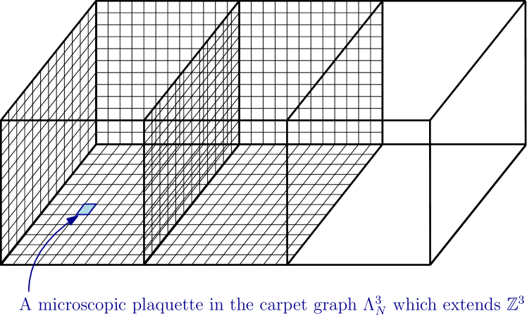
Figure 1:

For $Q\colon G\to[0,\infty)$, let $\mu_{Q,N}$ be the probability measure on $G^{E_{N}}$ defined by [eq:LGTN] μ_Q,N(​dU) = Z_Q,N^-1 ∏_p∈P_NQ(U_p) ​dU . The difference between (LABEL:eq:LGT) and (LABEL:eq:LGTN) is that the product in the latter is over $p\in P_{N}$.

Remark 1.2

Every $U\in G^{E_{N}}$ canonically defines an element of $U\in G^{E}$ by taking ordered products along edges. Let $\pi_{N}\colon G^{E_{N}}\to G^{E}$ denote this projection.

Definition 1.3 (Villain action)

For $\beta>0$, define $V_{\beta}\colon G\to(0,\infty)$ by V_β(x) = e^12β^-1Δ(x) , where $\Delta=\sum_{a}T^{a}T^{a}$ is the Laplace–Beltrami operator on $G$.

Example 1.4 (Abelian Villain action)

When $G=U(1)=\mathbb{S}^{1}$, then the Villain interaction reads as follows: for any $\theta\in[0,2\pi)$,

$$V_{\beta}(\theta)=\frac{1}{Z}\sum_{m\in\mathbb{Z}}\mathop{\mathrm{exp}}\nolimits(-\frac{\beta}{2}(\theta+2\pi m)^{2})\,.$$

The following is our main result.

Theorem 1.5

Suppose $p_{N}$ satisfies Assumption 2.1 below. Then (π_N)_* μ_p_N,N →μ_V_β in total variant distance.

In the special case of Abelian symmetry, $G=U(1)$, let us introduce a lattice gauge theory with edge-dependent Villain interactions on $\Lambda^{d}=\{x\in\mathbb{Z}^{d}\,:\,|x|_{\infty}\leq L\}$. Let $\bar{\beta}=(\beta_{e})_{e\in E(\Lambda^{d})}$ be a field of non-negative coupling constants. We define the Villain lattice gauge theory with coupling constants $\bar{\beta}$ to be μ_V, ¯β(​dU) = Z_V, ¯β^-1 ∏_p∈P(Λ^d) e^12 β_e^-1 Δ(U_p) ​dU

Corollary 1.6

When $G=U(1)$, all Wilson loop observables are monotone in the coupling constants $\bar{\beta}=(\beta_{e})_{e\in E(\Lambda^{d})}$ assigned to edges.

Proof.

This monotony is known for Wilson($=$XY) lattice gauge theory on any graph thanks to the Ginibre inequality [ginibre1970general]. By using the carpet graph limit used in Section LABEL:s.Proof together with the fact that Wilson loop observables do not depend on any edges in $E_{N}\setminus\tilde{E}_{N}$ (see the notations in Section LABEL:s.Proof which contains the proof Theorem 1.5), we obtain the desired monotony.  

Remark 1.7

It is nicely explained, for example in [van2023duality], that one can deduce such monotonies readily from the Ginibre inequality (without considering such geometric limits via cable/carpet graphs) for any interaction $\theta\mapsto\mathop{\mathrm{exp}}\nolimits(-U(\theta))$ which is such that $\theta\mapsto-U(\theta)$ is positive definite (i.e. all its Fourier coefficients $\{-\hat{U}(k)\}_{k\neq 0}$ are non-negative). Unfortunately, it can be checked that

$$\theta\mapsto\mathop{\mathrm{log}}\nolimits{\left(\sum_{m\in\mathbb{Z}}\mathop{\mathrm{exp}}\nolimits(-\frac{\beta}{2}(\theta+2\pi m)^{2})\right)}$$

is not positive definite. Therefore, the present limiting procedure seems to be a necessary step in order to prove the monotony property stated in Corollary 1.6.

1.4 Idea of proof.

The proof handles the following two main difficulties which are addressed respectively in Sections LABEL:s.commute and LABEL:sec:transition:

1. Restoring some commutativity. When the gauge group $G$ is non-Abelian, we may fear (we did at least!) that we may not be able to split the interaction over plaquettes into microscopic interactions over many plaquettes. For example, it is well known that when $G$ is non-Abelian, we cannot express Wilson loop observables as a product over a spanning surface of microscopic loop observables. Also, spanning trees, which can be used to remove gauge freedom, help to reduce the problem when $d=2$ to a problem about random walks in a group but this is in general not the case when $d\geq 3$ (though see [chatterjee2016leading] where spanning trees are used in the form of axial gauge fixing for any $d\geq 2$). It turns out we can still restore enough commutativity thanks to the straightforward Lemma LABEL:l.easy and ideas from planar (2D) gauge theory in the form of Lemma LABEL:lem:reduction.

2. Strong convergence of the heat-kernel. The second difficulty which naturally arises is more analytical. When a plaquette $p$ is divided into $N^{2}$ small plaquettes each with inverse temperature $\beta_{N}=N^{2}\beta$, we end up with the heat-kernel on the Lie Group $G$ after $T=N^{2}$ steps of a random walk $G$ with small random displacements. The convergence of this random-walk heat-kernel towards the heat-kernel of the limiting Brownian motion on the Lie-Group $G$ is well known (see for example [Stroock_Varadhan_73, jorgensen1975central]). But it is only established in the weaker notion of convergence in distribution. In the present situation, each plaquette contributes such a heat-kernel and we need to control products of these heat-kernels. Since such products behave very poorly under weak convergence, we crucially need to upgrade the notion of convergence of RW-heat-kernels to the $G$-valued Brownian motion heat-kernel. This is the purpose of Section LABEL:sec:transition which is greatly inspired by [Hebisch_Saloff_Coste_93] and [CS23].

Acknowledgments. The authors wish to thank Fabrice Baudoin, Diederik van Engelenburg and Avelio Sepúlveda for useful discussions as well as the University of Geneva (Unige) where this work has been initiated in Spring 2023. I.C. acknowledges support from the EPSRC via the New Investigator Award EP/X015688/1. C.G. acknowledges support from the Institut Universitaire de France (IUF), the ERC grant VORTEX 101043450 and the French ANR grant ANR-21-CE40-0003.

2 Assumption on actions

Denote by $\mathfrak{g}$ the Lie algebra of $G$ and equip $\mathfrak{g}$ with the inner product ${\langle X,Y\rangle}=-\operatorname{Tr}(XY)$, which is $\mathrm{Ad}$-invariant. Let $D$ denote the dimension on $\mathfrak{g}$ and let $T^{1},\ldots,T^{D}$ be an orthonormal basis of $\mathfrak{g}$. Recall that a function $f\colon G\to\mathbb{R}$ is called a class function if $f(xyx^{-1})=f(y)$ for all $x,y\in G$ and is called symmetric if $f(x)=f(x^{-1})$ for all $x\in G$.

Assumption 2.1

Let $p_{N}\colon G\to[0,\infty)$ be a symmetric class function such that $\int_{G}p_{N}(x)\mathop{}\!\mathrm{d}x=1$. (Recall $\mathop{}\!\mathrm{d}x$ stands for the Haar measure on $G$). We make the following two assumptions.

1. $p_{N}^{\star N^{2}}(x)\mathop{}\!\mathrm{d}x\to V_{\beta}(x)\mathop{}\!\mathrm{d}x$ in distribution as $N\to\infty$.

2. There exist $r,\theta,\Theta>0$ such that, for all $N\geq 1$, we can write $p_{N}(x)=Z_{N}^{-1}e^{-S_{N}(x)}$ with the property that ∀x∈B_N^-1 r=def{x∈G :  ϱ(x,1_G)¡N^-1 r} : S_N(x) ≤ΘN^2ϱ(x,1_G)^2 and ∀x∈G : S_N(x) ≥θN^2 ϱ(x,1_G)^2 , where $\varrho$ is the geodesic distance on $G$ induced by ${\langle\cdot\rangle}$ and $1_{G}$ is the identity element of $G$.

Example 2.2 (Wilson action)

Define $W_{\beta}\colon G\to(0,\infty)$ by W_β(x) = Z^-1exp(-β(ReTr(1_G-x) )) where $Z$ is such that $\int_{G}W_{\beta}=1$. Define $p_{N}=W_{N^{2}\beta}(x)$. Then by [CS23, Example 9.16], $p_{N}$ satisfies Assumption 2.1(b). Assumption 2.1(a), i.e. that $p_{N}^{\star N^{2}}(x)\mathop{}\!\mathrm{d}x\to V_{\beta}(x)\mathop{}\!\mathrm{d}x$ in distribution, follows from Proposition 2.6 below.

Example 2.3 (Manton action)

Define $M_{\beta},\colon G\to(0,\infty)$ by M_β(x) = Z^-1exp(-βϱ(x,1)^2) where $Z$ is such that $\int_{G}M_{\beta}=1$. Then $p_{N}\stackrel{{\scriptstyle\mbox{\tiny def}}}{{=}}M_{N^{2}\beta}(x)$ trivially satisfies Assumption 2.1(b). Assumption 2.1(a) follows from Proposition LABEL:prop:Manton_conv below.

We next give a general way to verify the convergence $\mathbb{P}_{N}^{\star N^{2}}\to V_{\beta}(x)\mathop{}\!\mathrm{d}x$ in distribution. Let $\xi^{1},\ldots,\xi^{D}\in{\mathcal{C}}^{\infty}(G,\mathbb{R})$ be local exponential coordinates of the first kind associated to the basis $T^{a}$, i.e. the map $\xi\colon G\to\mathfrak{g}$ defined by ξ(x) =def∑_a=1^D ξ^a(x) T^a satisfies $e^{\xi(x)}=x$ for all $x$ in a neighbourhood of $1_{G}$. We assume without loss of generality that $\xi$ is odd, i.e. $\xi(x)=-\xi(x^{-1})$ (otherwise we can replace $\xi^{a}(x)$ by $\frac{1}{2}\xi^{a}(x)-\frac{1}{2}\xi^{a}(x^{-1})$).

Suppose $\mathbb{P}_{N}$ are probability measures on $G$, let $\mathbb{E}_{N}$ denote the associated expectations, and define B_N = E_N[ξ] , A^a,b_N = E_N[ξ^aξ^b] , 1≤a,b ≤D .

For $Q\colon G\to[0,\infty)$, let $Q^{\star k}$ denote the $k$-fold convolution of $Q$ with itself, i.e. Q^⋆k(x)=∫_G^k-1 Q(x_1)Q(x_1^-1 x_2) Q(x_2^-1x_3)…Q(x_k-1^-1 x) ​dx_1…​dx_k-1 . More generally, if $\mathbb{P}$ is a probability measure on $G$, we let $\mathbb{P}^{\star k}$ denote its $k$-fold convolution, which is just the law of the $k$-th step $X_{k}$ of the random walk on $G$ with $X_{0}=1_{G}$ and whose increments $X_{i-1}^{-1}X_{i}$ are i.i.d. and distributed by $\mathbb{P}$.

Lemma 2.4

Suppose $\mathop{\mathrm{lim}}_{N\to\infty}\mathbb{P}_{N}(C)=0$ for every closed set $C\subset G$ such that $1_{G}\notin C$. Suppose further that $NB_{N}\to 0$ and $NA^{a,b}_{N}\to A^{a,b}$ as $N\to\infty$.

Then $\mathbb{P}_{N}^{\star N}\to\mathbb{P}$ in distribution where $\mathbb{P}(\mathop{}\!\mathrm{d}x)=e^{{\mathcal{L}}}(x)\mathop{}\!\mathrm{d}x$ is the law at time $1$ of the $G$-valued diffusion with generator ${\mathcal{L}}=\frac{1}{2}\sum_{a,b=1}^{D}A^{a,b}T^{a}T^{b}$ (i.e. $e^{t{\mathcal{L}}}$ is the heat-kernel of ${\mathcal{L}}$).

Remark 2.5

This result does not require orthonormality of $T^{a}$ or compactness of $G$; it is a special case of a general “functional” central limit theorem for walks with independent increments that applies to any connected Lie group, see [Feinsilver78, Stroock_Varadhan_73, jorgensen1975central] or [Chevyrev18, Sec. 2.2], the notation of which we follow. It also follows from Wehn’s central limit theorem [Wehn_thesis, Wehn62, Grenander63], see also the survey [Breuillard_07].

Proposition 2.6

For the Wilson action from Example 2.2, we have

$$W_{N\beta}^{\star N}(x)\mathop{}\!\mathrm{d}x\to V_{\beta}(x)\mathop{}\!\mathrm{d}x$$

in distribution as $N\to\infty$.

Proof.

Let $\mathbb{P}_{N}(\mathop{}\!\mathrm{d}x)=W_{N\beta}(x)\mathop{}\!\mathrm{d}x$ and follow notation as above. By symmetry and the assumption that $\xi$ is odd, note that $B_{N}=0$.

There exists a connected domain $F\subset\mathfrak{g}$ such that $\mathop{\mathrm{exp}}\nolimits\colon F\to G$ is a bijection (e.g. $F=\{X\in\mathfrak{g}\,:\,\sigma(X)\subset(-i\pi,i\pi]\}$ where $\sigma(X)$ is the spectrum of $X$). Equip $\mathfrak{g}$ with the Lebesgue measure $\mathop{}\!\mathrm{d}X$ that assigns unit volume to the unit cube with respect to ${\langle\cdot,\cdot\rangle}$ (i.e. the map $\mathfrak{g}\ni\sum_{a}X^{a}T^{a}\mapsto\sum_{a}X^{a}e^{a}\in\mathbb{R}^{D}$ is a measure preserving isometry for the standard Lebesgue measure on $\mathbb{R}^{D}$). Let $J\colon F\to[0,\infty)$ denote the Jacobian of $\mathop{\mathrm{exp}}\nolimits$, i.e. the pushforward of $J(X)\mathop{}\!\mathrm{d}X$ via $\mathop{\mathrm{exp}}\nolimits$ is the Haar measure on $G$. Then [eq:xi2_Wilson] N E_N [ξ⊗ξ] = Z_N^-1 ∫_F N ξ(e^X)