The Quasar Catalogue for S-PLUS DR4 (QuCatS) and the estimation of photometric redshifts

Abstract

The advent of massive broad-band photometric surveys enabled photometric redshift estimates for unprecedented numbers of galaxies and quasars. These estimates can be improved using better algorithms or by obtaining complementary data such as narrow-band photometry, and broad-band photometry over an extended wavelength range. We investigate the impact of both approaches on photometric redshifts for quasars using data from S-PLUS DR4, GALEX DR6/7, and unWISE in three machine learning methods: Random Forest (RF), FlexCoDE, and Bayesian Mixture Density Network (BMDN). Including narrow-band photometry improves the root-mean-square error by 11% in comparison to a model trained with only broad-band photometry. Narrow-band information only provided an improvement of 3.8% when GALEX and WISE colours were included. Thus narrow bands play a more important role for objects that do not have GALEX or WISE counterparts, which respectively makes 92% and 25% of S-PLUS data considered here. Nevertheless, the inclusion of narrow-band information provided better estimates of the probability density functions obtained with FlexCoDE and BMDN . We publicly release a value-added catalogue of photometrically-selected quasars with the photo-z predictions from all methods studied here. The catalogue provided with this work covers the S-PLUS DR4 area ($\sim 3000\text{deg}^{2}$), containing 645 980, 244 912, 144 991 sources with the probability of being a quasar higher than, 80%, 90%, 95% up to $r<21.3$ and good photometry quality in the detection image. More quasar candidates can be retrieved from the S-PLUS database by considering less restrictive selection criteria.

1 Introduction

Quasars are known to be the most energetic objects in the Universe (Kormendy & Ho 2013). Since the first quasar discovery by Schmidt (1963), the number of confirmed quasars increased to almost a million. Among many surveys that have contributed to the discovery of new quasars, the Sloan Digital Sky Survey (SDSS; York et al., 2000) has provided the largest number of confirmed quasars with the SDSS-I/II/III/IV phases, including the extended Baryon Oscillation Spectroscopic Survey (eBOSS; Dawson et al. 2016). The SDSS DR16 quasar catalogue from DR16 (DR16Q; Lyke et al. 2020) includes objects from all SDSS programs and contains 920 110 spectroscopic observations of 750 414 quasars. The SDSS success in finding quasars is due to multiple efficient techniques for candidate quasar selection and redshift estimation based on optical and mid-infrared colours (see Myers et al. 2015 for an overview).

Information needed to select candidate quasars for follow-up spectroscopic observations is typically provided by photometric sky surveys. Furthermore, if adequate colours are available, quasars redshifts can be estimated using photometry alone, thus bypassing the need for expensive spectroscopic observations. Techniques to estimate redshifts using photometric observations (photometric redshifts or photo-zs) are well studied in the literature, but they remain an active research topic. There are two main approaches to photo-zs: SED (spectral energy distribution) template fitting (e.g. Salvato et al. 2009, Babbedge et al. 2004) and empirical methods based on training samples (e.g. Wu & Jia 2010, Brescia et al. 2013, Nakoneczny et al. 2021, Yang & Shen 2022), each with their own pros and cons. In general, machine learning as an empirical approach provides more accurate photo-z predictions than SED template fitting (e.g. Schmidt et al. 2020). However, the robust performance of such methods is limited to the parameter space of the training set, while SED template fitting has no such limitations (see Brescia et al. 2021 for further discussion).

In this work, we analyze the performance of photometric redshift estimates based on 12-band photometric data from the Southern Photometric Local Universe Survey (S-PLUS; Mendes de Oliveira et al. 2019). S-PLUS is a large-area sky survey that will cover $\sim$9300 deg² of the Southern Sky with the same optical system used in the Javalambre Photometric Local Universe Survey (J-PLUS; Cenarro et al. 2019). This optical system consists of seven narrow bands and five $ugriz$ broad bands ($griz$ are similar to the SDSS bands; Fukugita et al. 1996), providing effectively low-resolution spectra that are expected to improve photometric redshift estimates compared to those based on broad-band photometry alone. We also extend S-PLUS data with photometry from GALEX (Martin et al. 2005) and WISE (Wright et al. 2010) surveys to study how photo-z estimates improve due to an extended wavelength range compared to improvements due to the addition of narrow-band photometry. We focus here on photo-z techniques based on machine learning.

We tested three different and independent machine learning algorithms: Random Forest, FlexCoDE, and Bayesian Mixture Density Network. We discuss the advantages and disadvantages of each method, and in particular assess the importance of the narrow-band photometry for the photo-z regression. Using three independent methods allows us to check for consistency in the interpretation of our results. We provide a value-added catalogue of quasar candidates for spectroscopic follow-up with their assigned probabilities of being a quasar (obtained from the star/quasar/galaxy classification by Nakazono et al. 2021) and their estimated photometric redshifts from this work. Estimates from all three methods are provided separately in the catalogue.

This paper is organised as follows: data sets used to estimate photo-zs are described in Section 2 and photo-z methods are described in Section 3. We present our results in Section 4 and how to select quasar candidates in Section 5. Finally, our main findings are discussed in Section 6.

2 Photometric Surveys and Datasets

In this section, we describe three photometric surveys, S-PLUS, WISE and GALEX, that provided photometry for photo-z estimation. In addition, a reliable sample of known quasars with spectroscopic redshifts is needed for training supervised machine learning methods and we used the SDSS DR16Q quasar catalogue (Lyke et al., 2020). In Table 1, we list the bands used in this work together with their effective wavelength, width and magnitude depth.

2.1 The Southern Photometric Local Universe Survey (S-PLUS)

The S-PLUS survey is an ongoing survey that, by the end, will cover $\sim$9300 deg² of the Southern Sky with the T80-South telescope located at Cerro Tololo Interamerican Observatory (CTIO), Chile. The S-PLUS optical filter system includes five broad bands: $u$, $g$, $r$, $i$, $z$ (similar to the SDSS filter system, except for the $u$ band) and seven narrow-band filters: J0378, J0395, J0410, J0430, J0515, J0660 and J0861, centred on [OII], Ca H+K, H$\gamma$, G-band, Mgb triplet, H$\alpha$ and Ca triplet features, respectively (Marín-Franch et al., 2012).

We use aperture fluxes computed within a circular diameter of 3 arcsecs and corrected for the fraction of the flux falling outside this limit (see Almeida-Fernandes et al. 2022 for more details). The procedure for data reduction and calibration of S-PLUS Data Release 4 (DR4), used in this work, is the same as used for S-PLUS DR2 (Almeida-Fernandes et al., 2022) and DR3. The S-PLUS DR4 comprises $\sim$3000 deg², including the area from past S-PLUS data releases. There are 645 980, 244 912, 144 991 sources photometrically classified as quasars with 80%, 90%, and 95% probabilities in S-PLUS with $r<21.3$ and good photometry flag in the detection image (SEX_FLAGS_DET $=0$). We corrected the data for reddening using dust maps from Schlegel et al. (1998) and the extinction law from Cardelli et al. (1989)

In Fig. 1 we show the SEDs of five examples of quasars from our sample with redshifts of 1.639, 2.238, 2.516, 3.207, and 4.435. The figure shows how the S-PLUS SEDs are shaped when one or more emission lines fall in the region of a narrow band. For instance, for $z\sim 1.63$, CIV is detected in J0410; for $z\sim 2.24$, Ly$\alpha$ is detected in J0395; for $z\sim 2.52$, Ly$\alpha$ is detected in J0430; for $z\sim 3.21$, Ly$\alpha$ is detected in J0515. At the red side of the optical wavelength range, S-PLUS has the J0660 narrow band with a magnitude limit of about 21.4 mag, which is deeper than all other narrow bands, and deeper than the $z$ band (see Table 1). Note from the bottom panel of Fig. 1 that the Ly$\alpha$ can be detected at the J0660 band in $z\sim 4.4$. Considering the large area of the southern sky that will be surveyed by S-PLUS, it will play an important role in finding quasar candidates that are under-represented in the SDSS spectroscopic sample.

2.2 The Wide-field Infrared Survey Explorer (WISE)

The Wide-field Infrared Survey Explorer (WISE; Wright et al. 2010) is an all-sky infrared survey that obtained photometry in four bands, in the wavelength range from 3.4 $\mu$m to 22 $\mu$m. In this work, we use the W1 and W2 bands from the unWISE catalog (Schlafly et al., 2019), with effective wavelengths 3.4 $\mu$m and 4.6 $\mu$m, respectively. The addition of these two infrared bands is known to significantly improve the performance of photo-zs for quasars (e.g. Bovy et al. 2012, Brescia et al. 2013, DiPompeo et al. 2015, Yang et al. 2017). WISE magnitudes are reported on the Vega System and their conversion to AB system is given by Eq. 1:

$$m_{\text{AB}}=m_{\text{vega}}+\Delta{m},$$ (1)

where $\Delta{m}=2.699$ and $\Delta{m}=3.339$ for W1 and W2, respectively. It is recommended to subtract a 4 mmag and a 32 mmag offset to the unWISE measurements (Schlafly et al., 2019). The Vega to AB offsets, as constants, do not affect machine learning photo-z methods as long as the feature space for the training set and for the unlabelled data are defined in the same way. Therefore, we do not convert these magnitudes to the AB system for this work. To apply our trained models in all sources observed in S-PLUS, we perform a CDS crossmatch with the unWISE catalogue within 2″. There are 75% out of 39 168 373 ($14<r<21.3$) sources with WISE counterpart in the S-PLUS DR4 area but only 54% have detection in the W2 band.

2.3 The Galaxy Evolution Explorer (GALEX)

The Galaxy Evolution Explorer (GALEX; Martin et al. 2005) is an all-sky ultraviolet survey that obtained photometry in two bands: far-UV (FUV) and near-UV (NUV). We retrieved data for both bands from GALEX DR6+7 (Bianchi et al., 2017) using CDS cross-match within 2″. The addition of these two UV bands is known to significantly improve the performance of photo-zs for quasars (e.g. Ball et al. 2008, Bovy et al. 2012, Brescia et al. 2013). There are 8% out of 39 168 373 ($14<r<21.3$) sources with GALEX counterpart in the S-PLUS DR4 area but only 2% have measurements in the FUV band.

Table 1: Optical filter system characterization of GALEX ($5\sigma$, Morrissey et al. 2007), S-PLUS (peak of the magnitude distribution at $\text{S/N}>3$, Almeida-Fernandes et al. 2022) and WISE (50% completeness at $\text{S/N}>5$, Schlafly et al. 2019). The effective wavelengths and widths are given in Angstroms, and the depths are given in AB magnitudes.

Survey	Band	Effective Wavelength	Width	Depth
GALEX	FUV	1528	442	19.90
	NUV	2310	1060	20.80
S-PLUS (broad bands)	u	3536	352	21.0
	g	4751	1545	21.3
	r	6258	1465	21.3
	i	7690	1506	20.9
	z	8831	1182	20.1
S-PLUS (narrow bands)	J0378	3770	151	20.4
	J0395	3940	103	19.9
	J0410	4094	201	20.0
	J0430	4292	201	20.0
	J0515	5133	207	20.2
	J0660	6614	147	21.1
	J0861	8611	408	19.9
WISE	W1	34000	6600	20.72
	W2	46000	10400	19.97

(a)

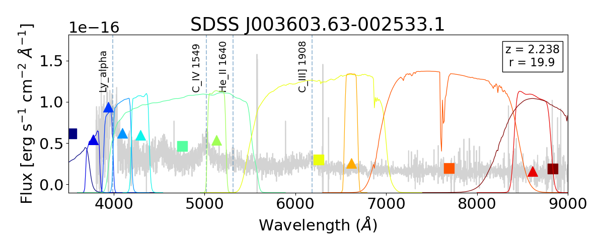
(b)

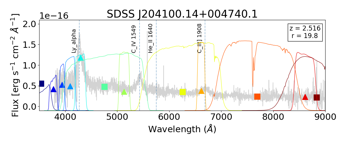
(c)

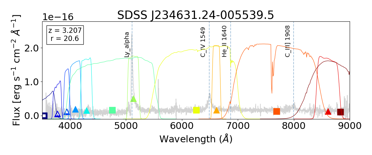
(d)

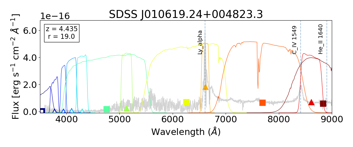
(e)

Figure 1: Spectral energy distribution of five quasars with spectroscopic redshifts of 1.639, 2.238, 2.516, 3.207, and 4.435 (top to bottom) showing an emission line being detected at an S-PLUS narrow band. In gray, we plot the spectra observed by the SDSS programs, with the identified emission lines being plotted in vertical dashed lines. The coloured triangles (squares) represent the flux measured in the S-PLUS narrow (broad) bands, from left to right: $u$, J0378, J0395, J0410, J0430, $g$, J0515, $r$, J0660, $i$, J0861, $z$. The filter responses are shown accordingly. Empty triangles/squares represent the error in AB magnitude above 0.5 or non-detection at that particular band.

2.4 Spectroscopic quasar sample

We cross-matched SDSS DR16Q with S-PLUS DR4 within 1″ radius, using data from the SDSS Stripe 82 equatorial region for our analysis ($\sim$300 deg²) resulting in 33 151 matches. Stripe 82 region dominates the current overlap between SDSS DR16Q and S-PLUS DR4, and represents the best-studied region in the SDSS footprint. We selected a total of 33 151 quasars with $r\leq 22$ and $z\leq 5$ for our analyses, which were cross-matched with unWISE and GALEX within 2″. A fraction of 93.1% and 85.9% out of 33 151 have detection in W1 and W2 bands from unWISE, respectively. For GALEX, only 30.8% and 11.1% have detection in NUV and FUV bands, respectively. Note that GALEX does not provide full sky coverage and therefore some of the missing-band values are due to non-observation. Ideally, non-detection and non-observation cases should be distinguished in the training process but determining the exact fraction of non-observation is not a trivial task. For the time being, we treat all non-observation missing values as they were non-detection (see §3.4 for further details).

3 Methods

In this work, we assess the importance of narrow-band photometry in improving the quality of quasar photo-z’s predictions. First, we discuss how much is the photo-z prediction improved when narrow-band photometry is added into a feature space that only contains broad-band photometry. In order to answer this question, we compare single-point estimates from Random Forest experiments trained with fixed hyperparameters and datasets using two different feature colour spaces:

• broad: $u-r$, $g-r$, $r-i$, $r-z$

• broad+narrow: the above four broad-band colours extended with the following seven narrow-band colours: $J0378-r$, $J0395-r$, $J0410-r$, $J0430-r$, $J0515-r$, $r-J0660$, and $r-J0861$.

We then discuss how the improvement factor changes when the GALEX and WISE broad-band photometry is also available. Similarly, as before, we compare two experiments trained with the following feature spaces:

• broad+GALEX+WISE: $u-r$, $g-r$, $r-i$, $r-z$, $FUV-r$, $NUV-r$, $r-W1$, $r-W2$

• broad+GALEX+WISE+narrow: the above eight broad-band colours extended with the same seven narrow-band colours as in the first case.

As GALEX and WISE bands improve photo-z’s predictions even when narrow-band colours are not included (see Section 4), we only consider the broad+GALEX+WISE and broad+GALEX+WISE+narrow feature spaces for further analyses. Testing three independent methods allows us to check the consistency of our conclusions about the importance of narrow-band photometry. Moreover, different methods can generally learn different patterns from the data and thus we also evaluate an ensemble of the three methods. Lastly, we also estimate photo-z’s probability density functions (PDFs) using FlexCoDE and Bayesian Mixture Density Network.

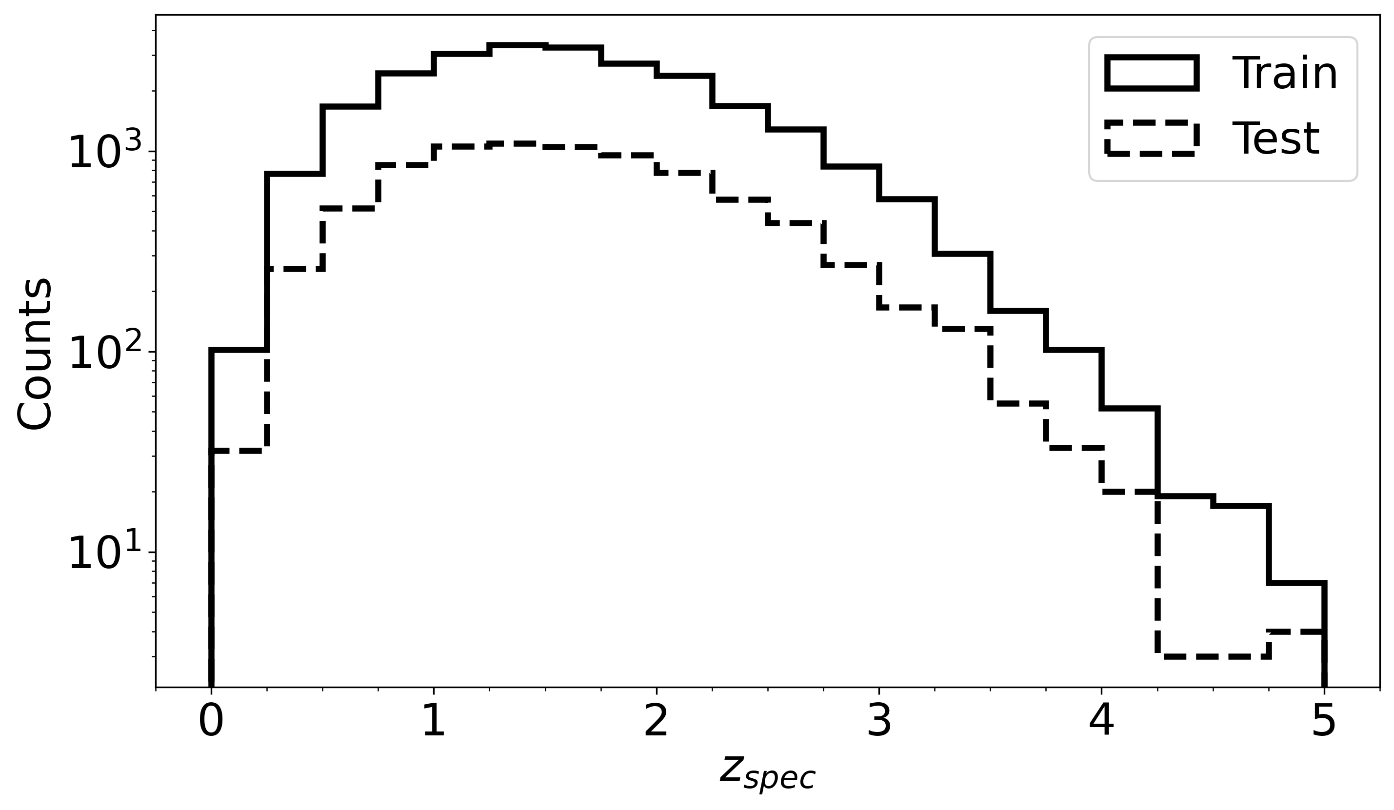
Figure 2: Distributions of spectroscopic redshift for the training and testing samples.

The quasar sample described in Section 2 is randomly split into training (75%) and testing (25%) sets. Their spectroscopic redshift distribution is shown in Fig. 2. Note that there are only few objects in the testing set for $z>4.2$, which may affect the performance estimation in this range. Here we introduce the methods used in this work: Random Forest (§3.1), FlexCoDE (§3.2), and Bayesian Mixture Density Network (§3.3). In §3.4 we discuss how we handled missing-band values and outliers. Finally, in §3.5 we discuss the metrics considered in this work to evaluate our model performance.

3.1 Random Forest

Random Forest (RF) is a non-parametric method that is robust to outliers, noise and over-fitting. Moreover, it is fast-learning, and, in some sense, interpretable due to the computation of feature importance. These characteristics and its known ability to provide high accuracy in diverse fields of study make RF an attractive algorithm. Since RF has been extensively used in astronomy, for more details we simply refer the reader to Breiman (2001). Regarding the specific task of estimating photometric redshifts, please see: Carliles et al. 2010 (galaxies), Henghes et al. 2021 (galaxies), and Nakoneczny et al. 2021 (quasars).

We use the Python implementation of RF in scikit-learn (version 1.1.3) package. We utilized the complete colour space (broad+GALEX+WISE+narrow) to run a grid search, resulting in the following configuration: n_estimators$=$400, min_samples_split$=$2, min_samples_leaf$=$2, max_depth$=$None, bootstrap$=$True. The photometric redshift is estimated as the mean value of the 400 predictions. We set random_state to 47 for all processes, in order to enable reproducibility. The remaining hyperparameters were kept at default values of scikit-learn v1.3.0. In this work, we do not provide an estimated probability density function for the photometric redshift with RF.

3.2 FlexCoDE

FlexCoDE (Flexible Nonparametric Conditional Density Estimation; Izbicki & Lee 2017; Dalmasso et al. 2020) is a non-parametric method that estimates conditional densities. FlexCoDE was applied to estimate photometric redshift distributions in the mock data produced for Vera Rubin Observatory’s LSST (Schmidt et al., 2020), providing the best Conditional Density Estimation (CDE) loss (see §3.5 for details) among several other methods. It is implemented in R (Izbicki & Pospisil 2019, the implementation used in this work), and Python (Pospisil et al., 2019).

Let $f(z|\textbf{x})$ be the probability density function of the redshift $z$ of a quasar with photometric covariates x. The key idea of FlexCoDE is to project $f(z|\textbf{x})$ on an orthonormal basis $(\phi_{i})_{i\in\mathbb{N}}$ (we use the Fourier basis):

$$f(z|\textbf{x})=\sum_{i\in\mathbb{N}}\beta_{i}(\textbf{x})\phi_{i}(z),$$ (2)

where $\beta_{i}(\textbf{x})$ are the expansion coefficients. By construction, these coefficients are given by

$$\beta_{i}(\mathbf{x})=\langle f(\cdot|\mathbf{x}),\phi_{i}\rangle=\int_{\mathbb{R}}\phi_{i}(z)f(z|\mathbf{x})dz=\mathbb{E}[\phi_{i}(Z)|\mathbf{x}],$$ (3)

and thus each coefficient $\beta_{i}$ can be estimated by regressing $\phi_{i}(Z)$ on x using the spectroscopic sample. In this paper, we use Random Forests to estimate each of these coefficients. The estimated density is then given by $\hat{f}(z|\mathbf{x})=\sum_{i=1}^{I}\hat{\beta_{i}}(\mathbf{x})\phi_{i}(z)$, where $I$ is a hyperparameter that defines the total number of expansion coefficients in the model. In practice, we choose the value of $I$ that minimizes the CDE loss function computed on a validation set (Equation 9). The single-point estimate is derived as the mode of the estimated probability density function.

3.3 Bayesian Mixture Density Network

We call as Bayesian Mixture Density Network (BMDN) the combination of two types of architectures: a Bayesian Neural Network (Bishop, 1997) and a Mixture Density Network (Bishop, 1994). BMDN is similar to a Dense network, where all neurons from one layer are connected to all neurons in the previous and following layers. The strength of these connections is given by weights, represented as single values.

In the Bayesian framework, these single-value weights are replaced by probability distributions. In our case, we assume a Gaussian distribution. For the implementation, we used the Tensorflow Probability (Dillon et al., 2017). The Mixture Density section of the network is what allows the estimation of distributions as output. This combination of architectures enables the network to represent arbitrary probability distributions while also allowing for an estimation of the epistemic (due to the model) and aleatoric (due to the data collection process) uncertainties, and provides a way to deal with the colour-redshift degeneracy (see §4.2). The architecture used in this work is shown in Fig. 3.

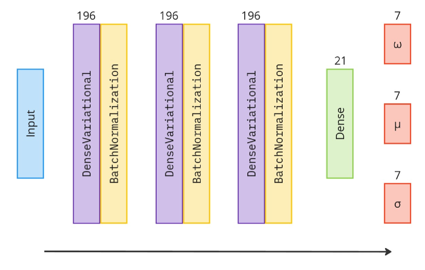
Figure 3: Architecture of the Bayesian Mixture Density Network. The input layer is followed by three blocks of DenseVariational and BachNormalization layers and a Dense layer. The numbers represent the number of neurons in that layer. The output layer (a MixtureNormal, in red) returns 7 weights ($w$), means ($\mu$) and standard deviations ($\sigma$).

The MixtureNormal layer of the network outputs 7 Gaussian functions described by 2 parameters: the mean ($\mu$) and the standard deviation ($\sigma$). Each Gaussian has an associated weight ($w$), so the photo-z’s probability density function is a combination of these Gaussian functions. For each object, we also derive a single-point estimate by computing the mode of the estimated probability density function.

3.4 Dealing with missing-band values

Missing-band values are intrinsic to astronomical data. We assume that any missing data in a non-detection case is "missing not at random" (MNAR; see Rubin 1976 for more information). An example of MNAR is a high-redshift quasar that is not detected in the blue bands due to the Lyman Break (e.g., see the two bottom panels in Fig. 1). These missing values have physical meaning and cannot be ignored. For MNAR, the removal of objects from our training set (also known as the complete-case method), or the mean/median imputation would bias our models (Dong & Peng, 2013).

For tree-based methods (such as Random Forest and FlexCoDE), we can handle the non-ignorable missing-band values by replacing them with an arbitrary out-of-the-range value (e.g., 99). The colours are calculated after the missing-band replacements.

For the Bayesian Mixture Density Network, we first replace any missing-band values in S-PLUS by the minimum magnitude of a non-detection given in the error column for each band. Then, we standardize the data and re-scale them to the range [0,1], without taking into consideration the missing-band values in GALEX and unWISE. The last scaling process is motivated by the suggested procedure from Chollet (2017) of replacing missing features by zeros. Since this can only be done if the value zero is not meaningful for the problem, and since colours can have this value, we use this second scaling function to shift the distribution. After the scaling processes, we replace any missing-band values in GALEX and unWISE by zeros.

3.5 Model Evaluation

Here we present the performance metrics considered in this work. Let $z$ be the (true) spectroscopic redshift and $\hat{z}$, the estimated photometric redshift (sometimes, especially in figures, we also refer to them as z${}_{\text{spec}}$ and z${}_{\text{phot}}$, respectively).

Defining $\delta z=z-\hat{z}$, $\delta z_{\text{norm}}=\delta z/(1+z)$ and considering $N$ being the number of evaluated objects, we define the following performance metrics for the single-point predictions:

• Root-mean-squared error:

  $$\sigma_{\text{RMSE}}=\sqrt{\frac{1}{N}\sum_{i=1}^{N}{(\delta z_{i})^{2}}},$$ (4)

• Normalized median absolute deviation:

  $$\sigma_{\text{NMAD}}=1.48\times\text{median}\Big{(}\frac{|\delta z-\text{median}(\delta z)|}{1+z_{\text{spec}}}\Big{)}$$ (5)

• Bias:

  $$\mu=\overline{\delta z}=\frac{\sum_{i=1}^{N}\delta z_{i}}{N},$$ (6)

• Fraction of objects with residual above a cutoff $c$:

  $$\eta_{c}=\frac{N_{|\delta z_{\text{norm}}|>c}}{N}.$$ (7)

The $\sigma_{\text{NMAD}}$ is commonly used to evaluate redshift estimates as it is less sensitive to outliers (Salvato et al., 2019). Photo-z single-point estimates are better when these metrics are closer to zero.

Now, let $\hat{f}$ be the estimated probability density function, and let $\hat{F}$ be the estimated cumulative density function. In order to evaluate the probability density functions estimated by FlexCoDE and Bayesian Neural Networks, we use the following metrics:

• Probability Integral Transform (PIT), which should be uniformly distributed if the density is well calibrated (Freeman et al., 2017; Polsterer et al., 2016; Zhao et al., 2021; Dey et al., 2022):

  $$PIT(\hat{f},z)=1-\hat{F}(z\>|\>\mathbf{x})=1-\int_{0}^{z}\hat{f}(z\>|\>\mathbf{x})dz,$$ (8)

• Conditional Density Estimate (CDE) loss function (Izbicki & Lee, 2016; Izbicki et al., 2017), $\hat{L}(f,\hat{f})$, which is an estimate of:

  $$L(f,\hat{f})=\int\int\left(f(z\>|\>\textbf{x})-\hat{f}(z\>|\>\textbf{x})\right)^{2}dzdP(\textbf{x}).$$ (9)

4 Results

In this section, we analyze the importance of the narrow-band photometry for estimating quasar photometric redshifts using RF, FlexCoDE, and BMDN, because different methods might learn different underlying relations between the colour space and the true redshift. We first use RF with a 5-fold cross-validation method to evaluate all feature spaces described in Section 3. After narrowing the possible choices of feature spaces, we then evaluate the single-point estimates of all the three methods (see §4.1). In §4.2 we evaluate the estimated probability density functions from FlexCoDE and BMDN. Finally, in §4.3 we show the feature importances obtained from the tree-based models.

4.1 Assessing the importance of narrow-band photometry

Here, we compare the performance of Random Forest experiments trained on different feature spaces with fixed hyperparameters and fixed training/validation sets. With the choice of feature spaces described in Section 3, we aim to provide insights into the importance of narrow-band photometry for this regression problem. The quantitative comparisons were done with $\sigma_{\text{RMSE}}$, $\sigma_{\text{NMAD}}$, $\mu$, $\eta_{0.15}$, and $\eta_{0.3}$ under a 5-fold cross validation scheme. These metrics are shown in Table 2.

Table 2: Performances from cross-validation with Random Forest algorithm in terms of the root-mean-squared error ($\sigma_{\text{RMSE}}$), normalized median absolute deviation ($\sigma_{\text{NMAD}}$), bias ($\mu$), and the fraction of sources with residual above 0.15 ($\eta_{0.15}$) and 0.3 ($\eta_{0.3}$). Standard deviations are typically of order 10^-3.

Colour space	$\sigma_{\text{RMSE}}$	$\sigma_{\text{NMAD}}$	$\mu$	$\eta_{0.15}$	$\eta_{0.3}$
broad	0.647	0.217	0.001	0.492	0.225
broad+narrow	0.576	0.179	0.001	0.428	0.185
broad+GALEX+WISE	0.425	0.102	-0.001	0.228	0.070
broad+GALEX+WISE+narrow	0.410	0.093	0.001	0.217	0.066

Table 3: This table shows the mean performance improvement in per cent due to the addition of narrow-band information for the subset of sources without GALEX (FUV and NUV) or WISE (W1 and W2) counterparts. Here we only compare broad+narrow and broad colour spaces. The improvements are slightly below the 11% ($\sigma_{\text{RMSE}}$) and 17% ($\sigma_{\text{NMAD}}$) calculated from Table 2. For completeness, we also show the results for the complementary subsets.

Sample Subset	Decrease in $\sigma_{\text{RMSE}}(\%)$	Decrease in $\sigma_{\text{NMAD}}(\%)$	Sample size
Without GALEX	9.6	14.1	3405$\sim$3478
With GALEX	15.6	25.4	1494$\sim$1567
Without WISE	9.2	16.5	288$\sim$301
With WISE	11.2	17.6	4642$\sim$4684

When narrow-band colours are added to the broad-band colour space, there is a decrease in the values of $\sigma_{\text{RMSE}}$ and $\sigma_{\text{NMAD}}$ by about 11% and 17%, respectively. As is discernible from Table 2, in all cases $\sigma_{\text{RMSE}}$ is much larger than $\sigma_{\text{NMAD}}$ due to the influence of outliers. The impact of outliers is also well-tracked through $\eta$ metrics. The $\eta_{0.15}$ metric decreased from 49% to 43%, while $\eta_{0.3}$ also decreased from 23% to 19%. The biases are sufficiently small for all cases with an order of $10^{-3}$.

These improvements are smaller than the improvements observed when GALEX and WISE colours are added to broad-band colours (i.e., without using narrow-band colours). As shown in Table 2, the extended wavelength range due to the addition of GALEX and WISE colours improve $\sigma_{\text{NMAD}}$ and $\eta_{0.15}$ metrics by as much as about a factor of two. When all the data are used, broad-band colours, GALEX and WISE colours and narrow-band colours, only slight additional improvements are observed. These improvements are visualized using the histograms of the residuals ($z_{\text{spec}}-z_{\text{phot}}$) in Fig. 4; the residual distribution is more concentrated around zero when information from all bands is included in our model. Figure 5 shows how $\sigma_{\text{RMSE}}$ and $\eta_{0.30}$ vary with the apparent magnitude $r$. The addition of narrow-band and/or GALEX and WISE colours improves the regression performance, especially for brighter objects.

Figure 4: Distribution of the residuals ($z_{\text{phot}}-z_{\text{spec}}$) from the Random Forest model trained with broad (blue), broad+narrow (orange), broad+GALEX+WISE (green), broad+GALEX+WISE+narrow (pink).

As discussed above, the addition of GALEX and WISE colours to broad-band colours improves the performance of photo-z more than the addition of narrow-band colours to broad-band colours. However, we emphasize that GALEX and WISE bands are effectively shallower than the S-PLUS bands and for faint objects, only narrow-band photometry is available, besides broad-band photometry. To address these cases where narrow-band photometry will play a more important role, we calculate the metrics on subsets of the validation folds that do not have GALEX or WISE counterparts (see Table 3). For $\sigma_{\text{RMSE}}$ the improvement is of an order of $\sim$9% for both cases. Regarding $\sigma_{\text{NMAD}}$, the improvement is 14.1% for sources without GALEX counterpart, and 16.5% for sources without WISE counterpart.

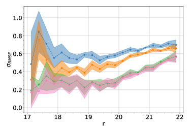
(a)

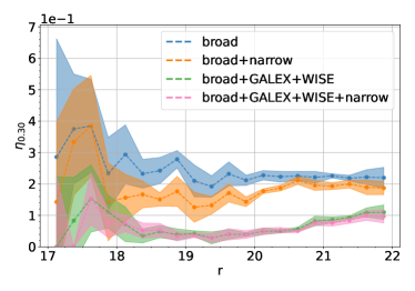
(b)

Figure 5: Median performance ($\pm$ 1$\sigma$) of Random Forest experiments trained on: broad, broad+narrow, broad+GALEX+WISE, and broad+GALEX+WISE+narrow. (a) $\sigma_{\text{RMSE}}$ per magnitude $r$ and (b) $\eta_{0.30}$ per magnitude $r$.

For further analyses that include FlexCoDE and BMDN, we only consider the broad+GALEX+WISE and broad+GALEX+WISE+narrow colour spaces. In Table 4 we show the metrics for all three methods; they all show small improvements from the addition of narrow bands regarding $\sigma_{\text{RMSE}}$, $\eta_{0.15}$, and $\eta_{0.30}$. There is an interesting behaviour observed for $\sigma_{\text{NMAD}}$: without narrow bands, all three methods have similar performance but when narrow bands are added, FlexCoDE and BMDN outperform RF method by a factor of two, approximately. On the other hand, RF method achieves about an order of magnitude smaller bias in comparison to FlexCoDE and BMDN for all models, except for the BMDN with the narrow bands. When we average the predictions from these three models, $\sigma_{\text{RMSE}}$ and $\eta_{0.30}$ are improved compared to each individual model. Note that the first two rows in Table 4 are not identical to the last two rows in Table 2 because the former is based on the testing set while the latter is based on the validation sets.

Table 4: Final performances calculated on the test set for Random Forest, FlexCoDE and Bayesian Mixture Density Network. The last two rows correspond to the performance when we average the single-point estimates from these three models. The best metric values are highlighted in bold.

	Feature Space	$\sigma_{\text{RMSE}}$	$\sigma_{\text{NMAD}}$	$\mu$	$\eta_{0.15}$	$\eta_{0.30}$
Random Forest	Without narrow bands	0.423	0.100	-0.002	0.225	0.068
	With narrow bands	0.408	0.090	0.003	0.220	0.066
FlexCoDE	Without narrow bands	0.477	0.084	0.044	0.222	0.084
	With narrow bands	0.455	0.039	0.016	0.209	0.078
Bayesian Mixture Density Network	Without narrow bands	0.458	0.083	0.025	0.212	0.074
	With narrow bands	0.427	0.048	$\mathbf{10^{-4}}$	0.187	0.068
Average	Without narrow bands	0.420	0.086	0.023	0.204	0.063
	With narrow bands	0.392	0.058	0.006	0.188	0.058

4.2 Probability density functions

Performance analyses from single-point estimates, however, do not account for the uncertainties in the photo-z predictions. It is expected that the photo-z’s PDFs can be multi-modal due to the colour-redshift degeneracy, which can be seen in Figure 6 for a random selection of 9 quasars from the test set at different ranges of spectroscopic redshift and magnitude. For instance, the colours of the quasar SDSS J232043.35-003049.3 are related to, approximately, two apart single-point estimates for FlexCoDE narrow-band model (i.e. broad+GALEX+WISE+narrow in pink curves), for which the PDF’s second highest peak is the one centred on the correct value. Nevertheless, the PDFs’ primary peak from FlexCoDE with the narrow-band model covers well the “true” redshift for most of the examples shown.

In comparison with BMDN, the FlexCoDE PDFs are generally more accurate for these particular model and examples. It is notable, however, that the PDFs are less certain on the predicted photo-z (i.e. distributions present more peaks) for the cases in the tail of the spectroscopic redshift distribution of the training sample beyond the $r$ magnitude depth of S-PLUS ($r>21.3$). This behaviour is also seen with the broad-band model (i.e. broad+GALEX+WISE, in green curves) and therefore might be related to the increasing photometric uncertainties at fainter magnitudes. Although the PDFs show more confusion at this range, the single-point prediction still agrees fairly well to the “true” redshift but only with the narrow-band model.

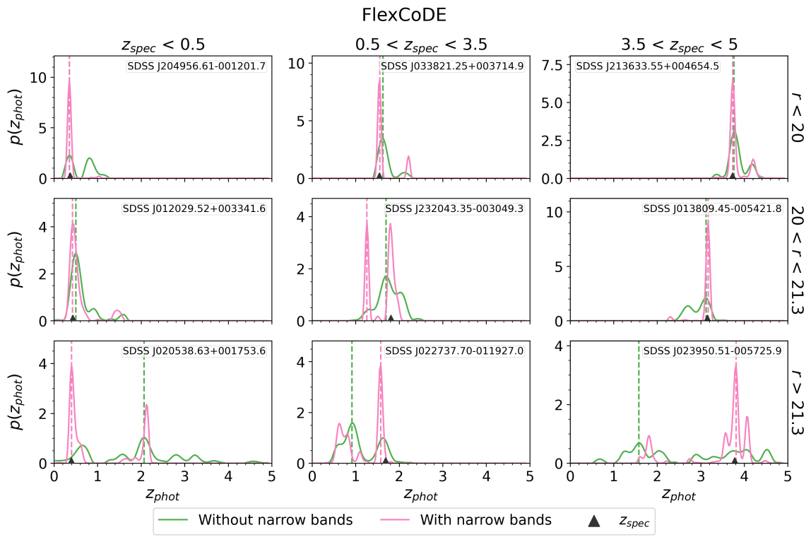
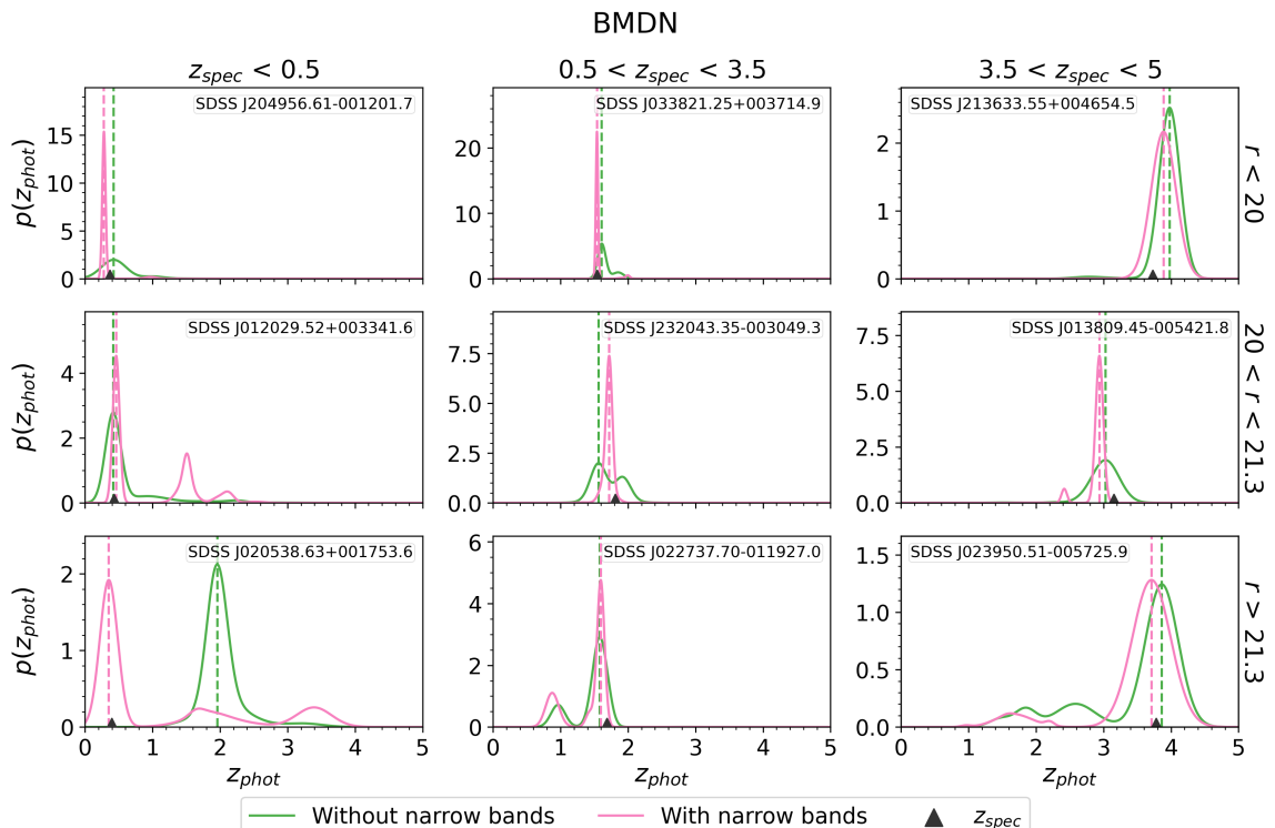
Figure 6: Density estimations $p(z)$ and single-point estimates from FlexCoDE and BMDN for the photometric redshift of 12 quasars sampled from the testing set. The spectroscopic redshift is pointed out with a triangle marker. Curves in green represent the model trained with broad+GALEX+WISE, while curves in pink represent the model trained with broad+GALEX+WISE+narrow. The single-point estimates are shown with dashed vertical lines.

Other quantitative comparisons should also be considered in order to evaluate the whole PDF information, such as the PIT distribution and the CDE loss function. As we have seen in Fig. 6, narrow-band model PDFs are generally sharper than broad-band model PDFs for both FlexCoDE and BMDN, suggesting that the predicted distribution is more precise (but not necessarily more accurate) when narrow-band information is included in the model. On the other hand, this could mean that the predictive uncertainties are not being properly accounted for and the distributions are sharper than they should be. The high edges (U-shape) of the PIT distributions shown in Fig. 7 agree with the suggestion of underdispersed PDFs. From this figure, we see that the narrow-band PDFs are more underdispersed than the broad-band PDFs. It then requires a better calibration of these PDFs that can either be achieved with a different machine learning architecture or with a re-calibration process (e.g. Dey et al., 2021), which is planned to be pursued in future work.

Nevertheless, we showed good evidence that the inclusion of narrow-band photometry is valuable for the precision of photometric redshift estimates. This is also supported by the calculated CDE losses, for which each individual PDF is evaluated (note that the loss can be estimated even if the true PDF is unknown). The CDE loss functions for FlexCoDE are -3.27 and -1.36 when trained with and without narrow bands, respectively. For BMDN, these values are -2.47 and -1.31. Therefore the FlexCoDE narrow-band model provided the best photo-z predictions during the testing process.

Given that the feature space and the training sample are the same, the differences in PDF shapes are model intrinsic. Different algorithms can learn different underlying patterns from the data, hence these PDFs could be combined to provide more powerful information. Assessing the possible combination of these PDFs is beyond the scope of this paper but we provide the PDFs from both methods in our value-added catalogue (see Section 5). Based on the CDE loss, the FlexCoDE trained with narrow bands delivered the best photo-zs and is our general recommendation for broad usage.

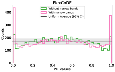
(a)

(b)

Figure 7: PIT distribution for (a) FlexCoDE trained without narrow bands (broad+GALEX+WISE) and with narrow bands (broad+GALEX+WISE+narrow); (b) BMDN trained without narrow bands and with narrow bands. The PDFs are considered well-calibrated if the distribution of PIT is described by a Uniform distribution.

4.3 Feature importances from tree-based models

In Fig. 8 we show the estimated feature importances for the Random Forest and the FlexCoDE models. In both models, the top two most important features for the quasar photo-z estimation are the same or strongly correlated. In first place, we have $r-W1$ for RF, and $r-W2$ for FlexCoDE. These two features are strongly correlated with Pearson correlation of 0.98. In the second place, the colour $u-r$ appears for both methods. These features ($r-W1$, $r-W2$, and $u-r$) measure the overall shape of the SED over the wide wavelength range. Beyond the second place, there is no interpretation agreement between the two models. While the first narrow-band ($J0378-r$) appears in 8th place for Random Forest, this same colour is the third most influential feature for FlexCoDE. This difference could be explained by the correlations between some of the colours, which can mislead the interpretation of the feature importances and does not necessarily mean that less important features are not relevant. Interestingly, not only do narrow-band colours have higher importances for FlexCoDE but also the overall importances are more equally distributed than RF. The importances shown in this figure might also be closely related to the relative depths of each band (see Table 1) but further investigation would be needed. Note that the interpretation of these importances is limited to understanding what features had the most influence in these particular prediction models and no physical or general conclusions can be taken from those. Nevertheless, there are good indications of the narrow-band importance in predicting more accurate photo-zs, as suggested by the FlexCoDE importances estimates and, especially, considering the CDE loss estimates discussed in the last section.

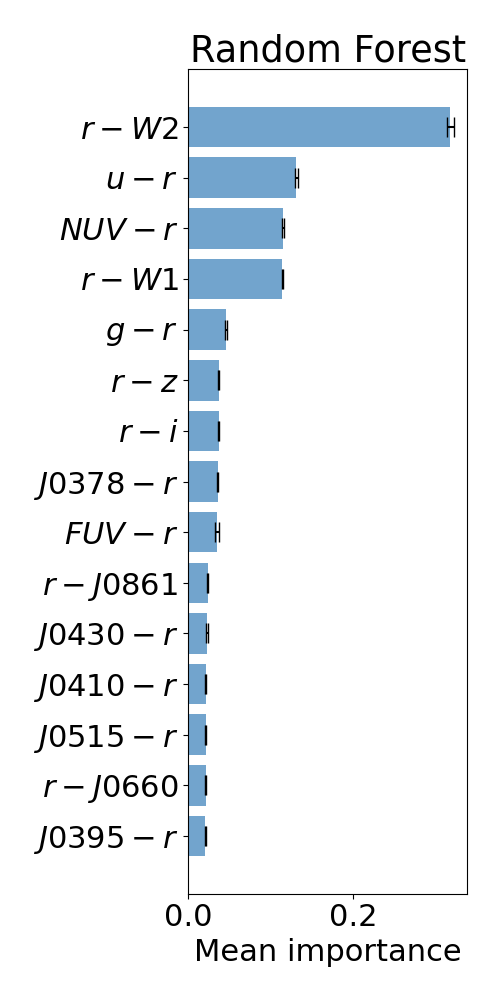
(a)

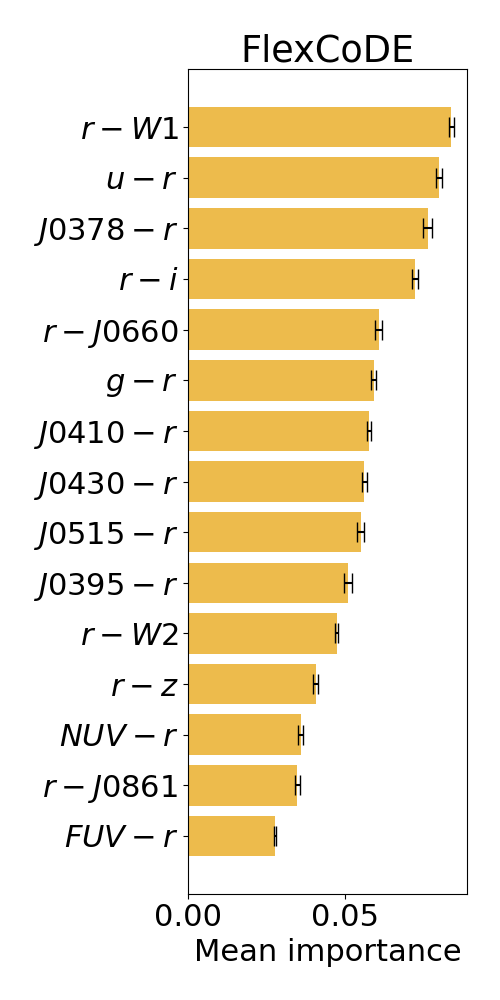
(b)

Figure 8: Average estimated importances and standard deviation for (a) Random Forest and (b) FlexCoDE.

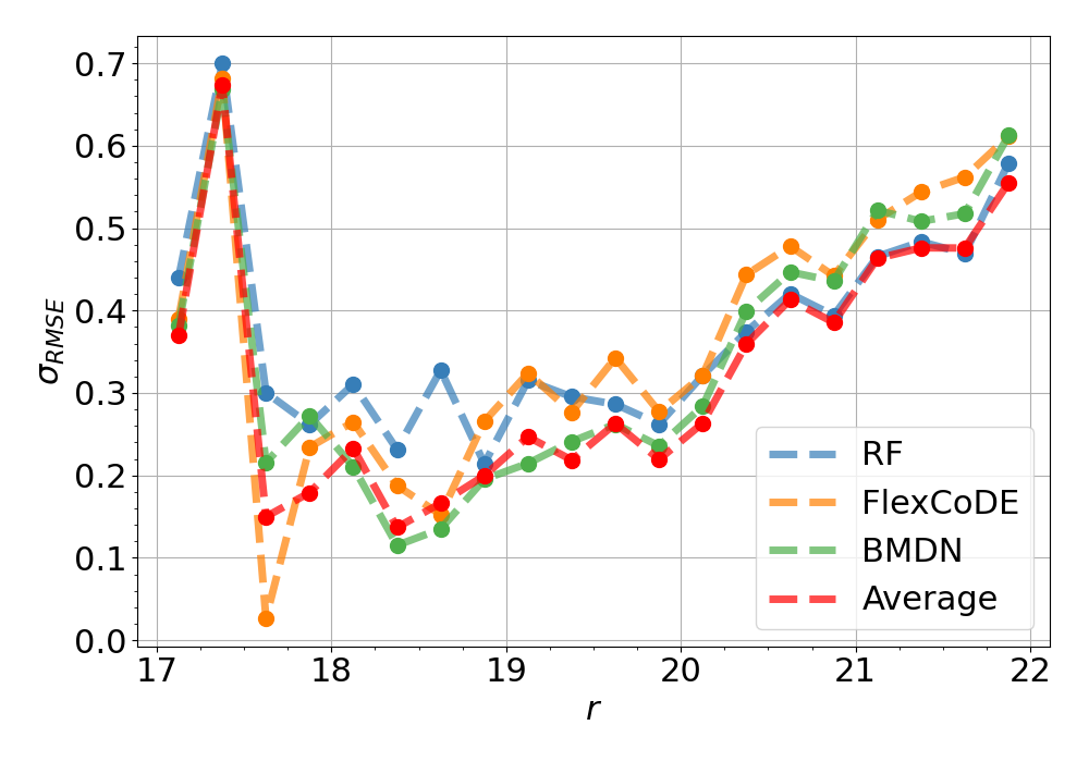
(a)

(b)

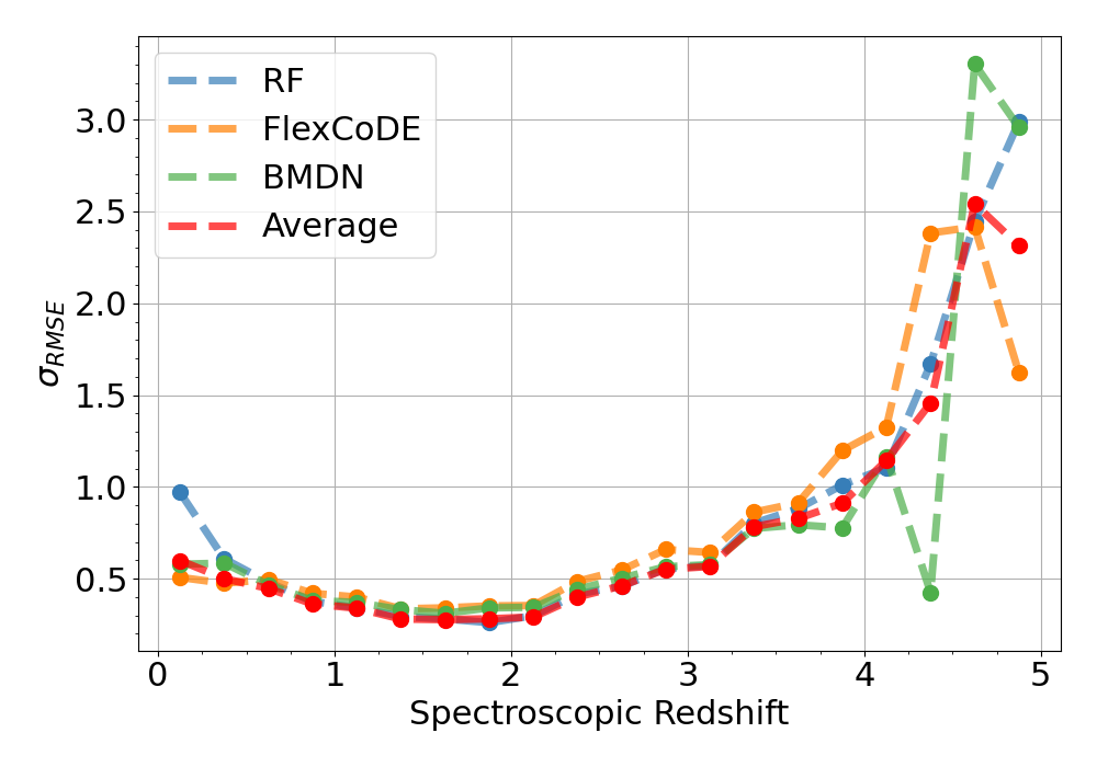
(c)

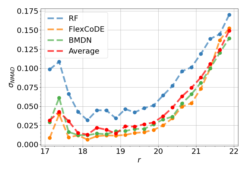
(d)

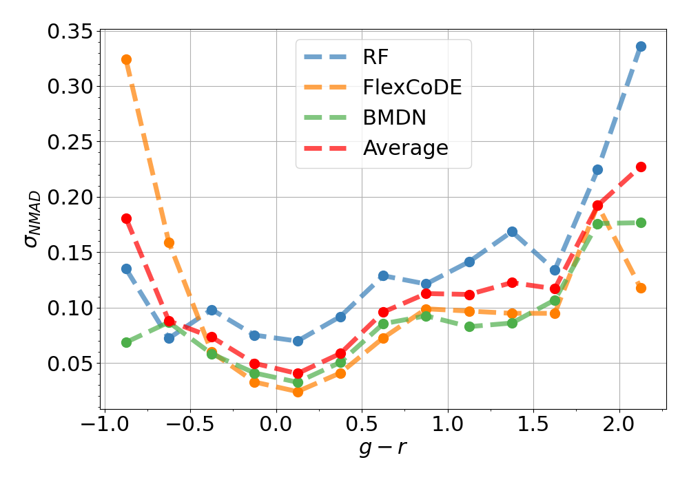
(e)

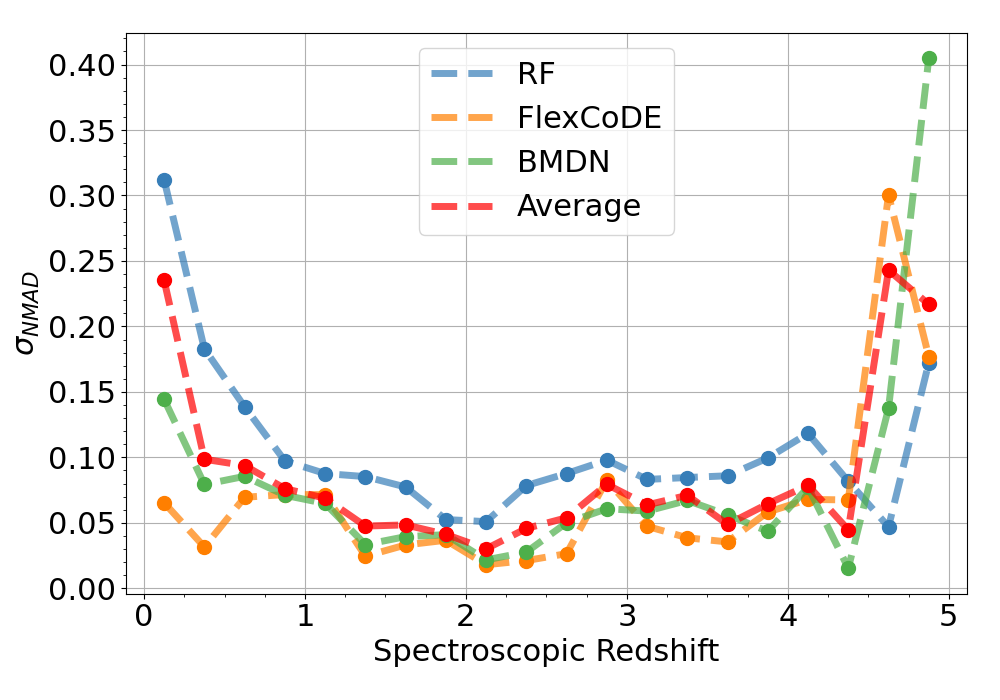
(f)

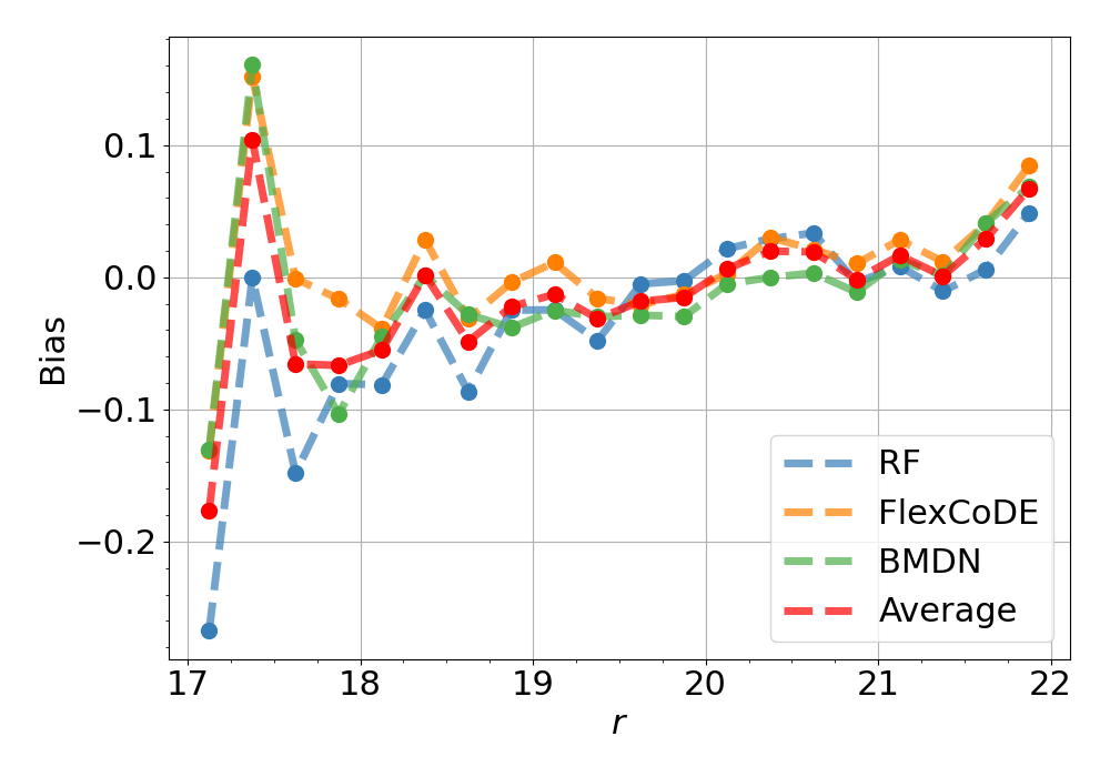
(g)

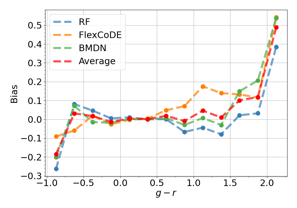
(h)

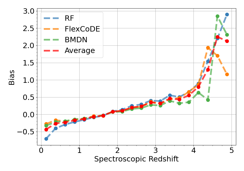
(i)

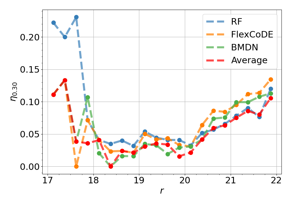
(j)

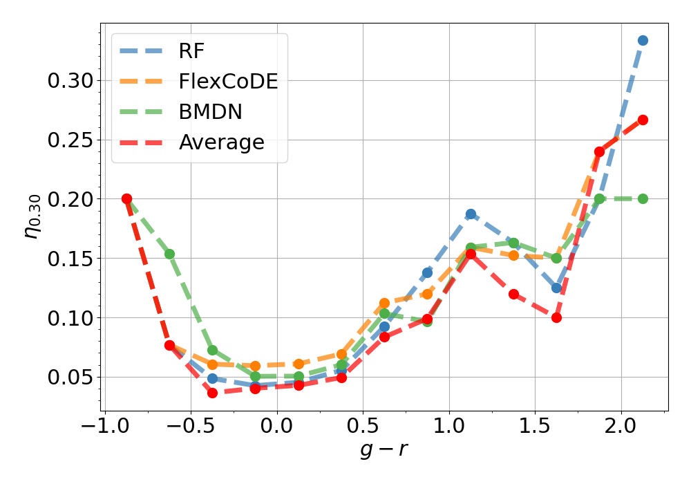
(k)

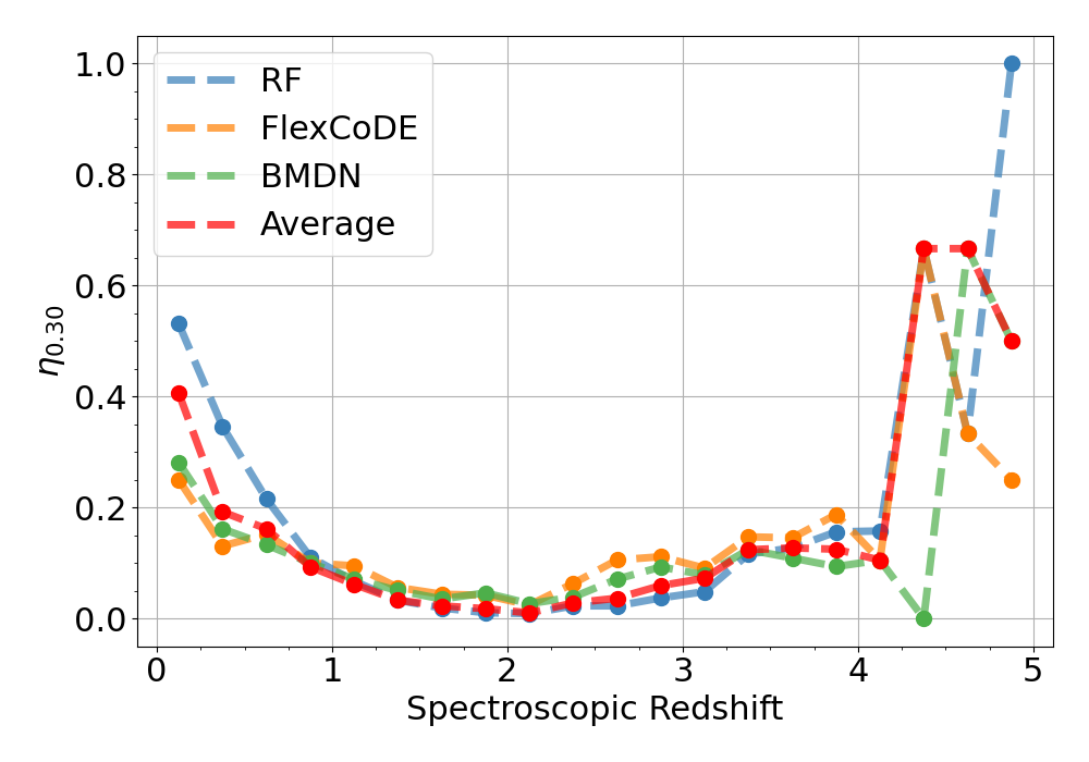
(l)

Figure 9: Performances in terms of $\sigma_{\text{RMSE}}$ (panels a, b, c), $\sigma_{\text{NMAD}}$ (panels d, e, f) , $\mu$ (panels g, h, i), and $\eta_{0.30}$ (panels j, k, l) per bin of magnitude r (left panels), colour g $-$ r middle panels), and spectroscopic redshift (right panels). The curves shown in the plots refer to the Random Forest (blue), FlexCoDE (orange), and Bayesian Mixture Density Network (green) trained with the broad+GALEX+WISE+narrow colour space. We show in red colour the performance when we average the predictions from the three methods.

5 QUCATS: The Quasar Catalogue for S-PLUS

The Quasar Catalogue for S-PLUS (QuCatS) provided with this paper contains 645 980 quasar candidates with classification probabilities above 80% up to the photometric depth of $r$ band ($r<21.3$) and good photometry quality in the detection image (SEX_FLAGS_DET $=0$) that comes from SExtractor. For the selection of quasar candidates, we use the star/quasar/galaxy classification probabilities from Nakazono et al. 2021 that were obtained with a Random Forest fit on S-PLUS and WISE magnitudes, and morphological parameters extracted from the S-PLUS images. Sources observed in the CCD borders that were observed in multiple fields were removed from this catalogue via an internal cross-match in RA and Dec within 1″. Our catalogue covers a total of 1414 fields from S-PLUS DR4, totalling approximately 3 000 $\text{deg}^{2}$ of the southern sky. This value-added catalogue is downloadable at https://splus.cloud/files/QuCatS_Nakazono_and_Valenca_2024.csv and its columns are described in Table 5. We do not make any cuts in photometric errors for the catalogue we provide in this paper but we advise users to make proper cuts for their specific science cases.

Below, we show an example of an ADQL query. The selection criteria can be easily modified in this query to retrieve more (or less) sources, where [columns] are defined by the user. We strongly recommend that a “WHERE det.Field = [field]” condition is added to this query in order to run one query per field, as big queries can overload the server. Note that one can relax the selection criteria and retrieve more quasar candidates from the S-PLUS database, as we derived photo-z estimations for all objects in each field regardless of their classification. Likewise, one can be more conservative with the selection criteria in order to improve the purity of the selected sample.

SELECT [columns] from dr4_vacs.dr4_qso_photoz as z
JOIN dr4_vacs.dr4_star_galaxy_quasar
as sqg on sqg.id = z.id
JOIN dr4_dual.dr4_dual_r
as r on r.id = z.id
JOIN dr4_dual.dr4_detection
as det on det.id = z.id
WHERE sqg.PROB_QSO >= 0.8 and
r.r_PStotal < 21.3 and
det.SEX_FLAGS_DET = 0

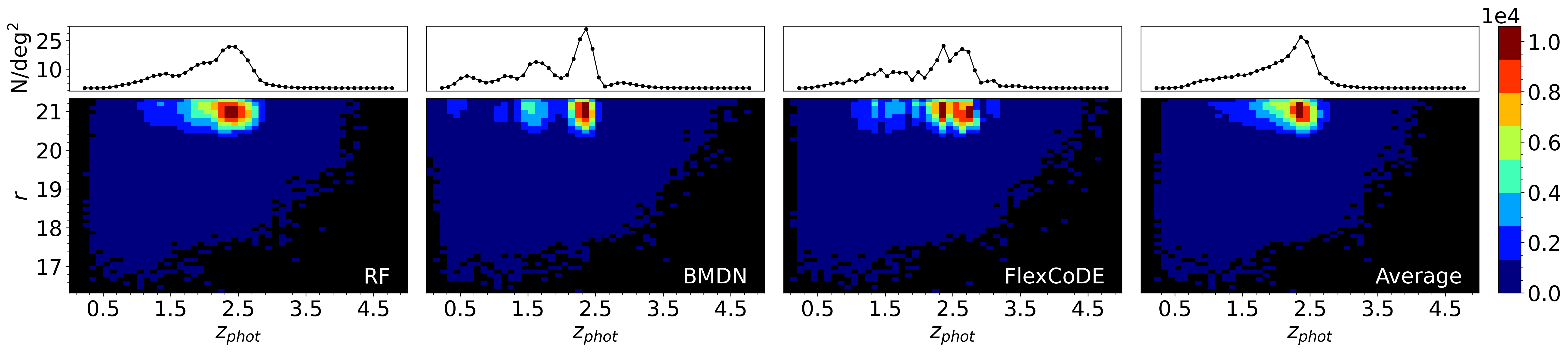
Figure 10: Density maps of photometrically selected quasar in S-PLUS DR4 with classification probabilities above 80% (Nakazono et al., 2021) and photometric redshift estimated with RF, BMDN, FlexCoDE, and the average of these three methods. Only sources with good photometry flag ($\texttt{SEX\_FLAGS\_DET}=0$) and $r<21.3$ are plotted. The colour map indicates the number of quasar candidates in bins of 0.1 for both apparent magnitude $r$ and photo-z. In the upper panels, we show the number of quasar candidates per squared degree for 0.1 bins of photo-z.

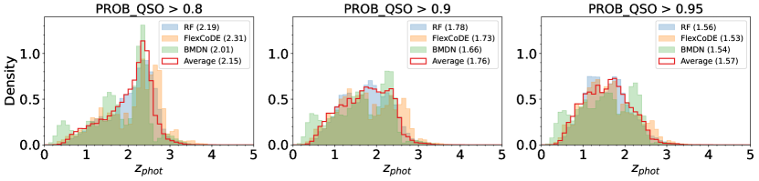
Figure 11: Distribution of photometric redshift for the sources that are photometrically classified as quasars in S-PLUS with a probability above 0.8, 0.9, and 0.95. Only sources with good photometry flag ($\texttt{SEX\_FLAGS\_DET}=0$) and $r<21.3$ are plotted. We can note that different estimation methods are leading to more alike photo-z distributions for high-confident quasar candidates ($\texttt{PROB\_QSO}>0.95$). The median of each distribution is given in the legend.

Density maps for the selected quasar candidates show a multi-modal distribution of photo-zs for BMDN and FlexCoDE, while RF deliver a smoother single-peak distribution (Fig. 10). In Fig. 11 we show the photo-z distribution for the quasar candidates in the catalogue provided in this paper with probability of being a quasar down to 0.8, 0.9, and 0.95. We can see that as we restrict our sample to more high-confident quasars, there is an increasing convergence among the photo-z distributions estimated by the different methods considered in this work. For high-confident quasar candidates (PROB_QSO $>$ 0.95), the distributions have medians at $z_{\text{phot}}\sim 1.55$.

Confirming which method is generalising better for unseen data is not trivial due to the intrinsic biases of using spectroscopic datasets to train the models. We advise users to use the information we provide in the catalogue with extra caution for the candidates that extrapolate the colour space distribution of the spectroscopic sample (for instance, see Fig. 12). Although we recommend FlexCoDE as it presented the lowest CDE loss, some science cases will demand certain requirements over specific magnitude/redshift ranges. For those, the performances per bin of magnitude $r$, colour $g-r$ and spectroscopic redshift allow for a more precise decision on which method to use (Fig. 9). Note that performances are poorer for lower ($z\lesssim 0.5$) and higher ($z\gtrsim 4.2$) probably due to the lack of objects in this range (see Fig. 2). Performances for brighter ($r\lesssim 17.5$) or bluer/redder ($|g-r|\gtrsim 0.5$) objects are also affected for the same reason (see Fig. 12). The performance decrease as magnitude increases is most likely related to increasing photometric uncertainties.

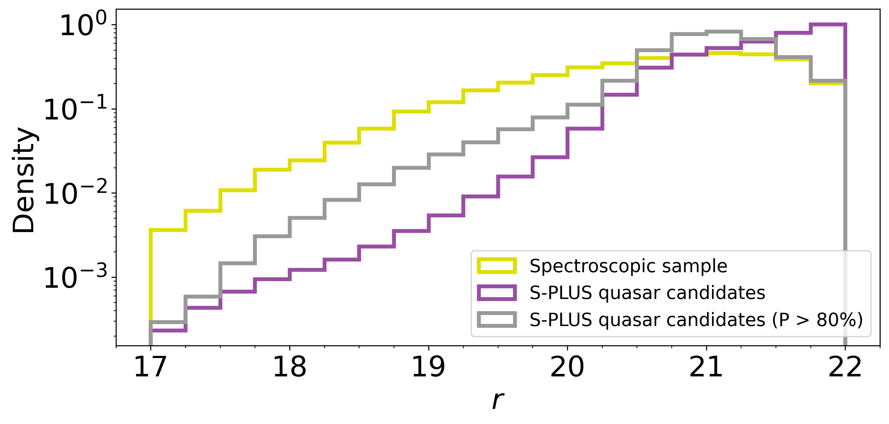
(a)

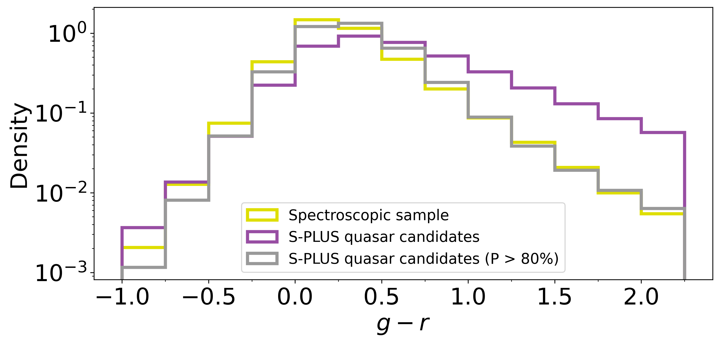
(b)

Figure 12: Distributions of (a) magnitude $r$ and (b) colour $g-r$ for the full spectroscopic sample (yellow), all quasar candidates in S-PLUS DR4 (purple), and high-confidence quasar candidates with probabilities down to 80% (grey). Sample sizes are 33 075, 15 908 524, and 1 078 149, respectively. The $g-r$ histogram comprises 99.2%, 93.1%, and 99.6% of each sample, respectively, in the plotted range.

Table 5: Description of the information provided in QuCatS. All columns here described are type float32. We also include useful information from the main survey (ID, Field, RA, DEC, PStotal magnitudes and their corresponding errors) and the classification value-added catalogues (PROB_QSO, PROB_STAR, PROB_GAL, model_flag). These extra columns are described in https://splus.cloud/documentation/DR4.

Column name	Description
z_rf	Photo-z estimated with RF
z_bmdn_peak	Photo-z estimated with BMDN (peak of the PDF)
z_flex_peak	Photo-z estimated with FlexCoDE (peak of the PDF)
z_mean	Average of {z_rf, z_bmdn_peak, and z_flex_peak}
z_std	Standard deviation of {z_rf, z_bmdn_peak, and z_flex_peak}
n_peaks_bmdn	Number of peaks for BMDN’s PDF
z_bmdn_pdf_weight_[1-7]	Weight of the [1-7]-th Gaussian distribution estimated with BMDN
z_bmdn_pdf_mean_[1-7]	Mean of the [1-7]-th Gaussian distribution estimated with BMDN
z_bmdn_pdf_std_[1-7]	Standard deviation of the [1-7]-th Gaussian distribution estimated with BMDN
z_flex_pdf_[1-200]	Probability for the [1-200]-th redshift within the interval [0.034, 4.913] estimated with FlexCoDE

6 Discussion and Conclusions

Up to this point, S-PLUS is the southern hemisphere survey that provided data within the largest area ($\sim$3000 square degrees in DR4) and the highest number of narrow bands. This makes S-PLUS a good laboratory for empirically evaluating the narrow-band importance in tasks such as photometric redshift (photo-z) regression. In this work, we compared three independent methods (Random Forest, FlexCoDE, Bayesian Mixture Density Network) trained with S-PLUS, GALEX, and WISE colours to obtain quasar photo-zs.

A reasonable improvement in quasar photo-z predictions was observed when narrow-band colours were included in the model over training with only broad-band colours. On the other hand, narrow-band information provided a small impact on the single-point estimates when GALEX and WISE colours were available. Thus narrow bands play a more important role for objects that do not have GALEX or WISE counterparts, which respectively makes 92% and 25% of the S-PLUS data. This conclusion is consistent with all tested algorithms.

As multi-modal photo-z distributions are expected due to the colour-redshift degeneracy, it is more appropriate to use the whole PDF information instead of single-point estimate summaries when evaluating performances. The models trained with narrow-band provide sharper distributions than the broad-band models, suggesting that the prediction uncertainties are not being properly accounted. This is confirmed through the PIT distributions, which show that the estimated PDFs are underdispersed for both FlexCoDE and BMDN (in this work, we do not analyse RF’s PDFs) and a re-calibration procedure is still needed. Nevertheless, for the scope of this paper, we have good indications that narrow-band photometry is helping to provide more accurate photo-zs, based on the CDE loss (which accounts for the PDF and not only the single-point estimates) and feature importance estimates for the tree-based models (especially from FlexCoDE).

Within this paper, we provide a value-added catalogue of photometric redshifts from all tested methods for 1414 fields ($\sim$3 000 $\text{deg}^{2}$) of S-PLUS DR4. We broadly recommend using the narrow-band FlexCoDE model as it presents the best CDE loss.

We conclude with a comment about the next-generation survey, the Rubin Observatory’s Legacy Survey of Space and Time (LSST; Ivezić et al. 2019). LSST will obtain broad-band photometry for billions of galaxies and millions of quasars. Given our analysis here, photometric redshift performance for these objects could be improved in two principal ways. First, the wavelength coverage could be extended over that accessible to Rubin Observatory using near-infrared space-based survey facilities such as Euclid (Laureijs et al., 2011) and Roman Space Telescope (Spergel et al., 2015). Alternatively, narrow-band photometry could be obtained after the initial 10-year broad-band survey is completed using the same telescope and camera as for LSST, but with an updated filter set as discussed in e.g., Yoachim et al. (2019) and Kahn et al. (2019).

Data Availability

The data underlying the machine learning training processes of this article are available in a GitHub repository at https://github.com/marixko/qucats_paper/tree/main/_survey/crossvalidation. Data products from this article are publicly available for queries at https://splus.cloud/.

References

- Almeida-Fernandes et al. (2022) Almeida-Fernandes F., et al., 2022, MNRAS, 511, 4590
- Babbedge et al. (2004) Babbedge T. S. R., et al., 2004, MNRAS, 353, 654
- Ball et al. (2008) Ball N. M., Brunner R. J., Myers A. D., Strand N. E., Alberts S. L., Tcheng D., 2008, ApJ, 683, 12
- Bianchi et al. (2017) Bianchi L., Shiao B., Thilker D., 2017, ApJS, 230, 24
- Bishop (1994) Bishop C., 1994, Workingpaper, Mixture density networks. Aston University
- Bishop (1997) Bishop C. M., 1997, J. Braz. Comput. Soc., 4
- Bovy et al. (2012) Bovy J., et al., 2012, ApJ, 749, 41
- Breiman (2001) Breiman L., 2001, Machine Learning, 45, 5
- Brescia et al. (2013) Brescia M., Cavuoti S., D’Abrusco R., Longo G., Mercurio A., 2013, ApJ, 772, 140
- Brescia et al. (2021) Brescia M., Cavuoti S., Razim O., Amaro V., Riccio G., Longo G., 2021, Frontiers in Astronomy and Space Sciences, 8, 70
- Cardelli et al. (1989) Cardelli J. A., Clayton G. C., Mathis J. S., 1989, ApJ, 345, 245
- Carliles et al. (2010) Carliles S., Budavári T., Heinis S., Priebe C., Szalay A. S., 2010, ApJ, 712, 511
- Cenarro et al. (2019) Cenarro A. J., et al., 2019, A&A, 622, A176
- Chollet (2017) Chollet F., 2017, Deep Learning with Python. Manning
- Dalmasso et al. (2020) Dalmasso N., Pospisil T., Lee A. B., Izbicki R., Freeman P. E., Malz A. I., 2020, Astronomy and Computing, 30, 100362
- Dawson et al. (2016) Dawson K. S., et al., 2016, AJ, 151, 44
- Dey et al. (2021) Dey B., Newman J. A., Andrews B. H., Izbicki R., Lee A. B., Zhao D., Rau M. M., Malz A. I., 2021, arXiv e-prints, p. arXiv:2110.15209
- Dey et al. (2022) Dey B., Zhao D., Newman J. A., Andrews B. H., Izbicki R., Lee A. B., 2022, arXiv preprint arXiv:2205.14568
- DiPompeo et al. (2015) DiPompeo M. A., Bovy J., Myers A. D., Lang D., 2015, MNRAS, 452, 3124
- Dillon et al. (2017) Dillon J. V., et al., 2017, TensorFlow Distributions, doi:10.48550/ARXIV.1711.10604, https://arxiv.org/abs/1711.10604
- Dong & Peng (2013) Dong Y., Peng J., 2013, SpringerPlus, 2, 222
- Freeman et al. (2017) Freeman P. E., Izbicki R., Lee A. B., 2017, Monthly Notices of the Royal Astronomical Society, 468, 4556
- Fukugita et al. (1996) Fukugita M., Ichikawa T., Gunn J. E., Doi M., Shimasaku K., Schneider D. P., 1996, AJ, 111, 1748
- Henghes et al. (2021) Henghes B., Pettitt C., Thiyagalingam J., Hey T., Lahav O., 2021, MNRAS, 505, 4847
- Ivezić et al. (2019) Ivezić Ž., et al., 2019, ApJ, 873, 111
- Izbicki & Lee (2016) Izbicki R., Lee A. B., 2016, Journal of Computational and Graphical Statistics, 25, 1297
- Izbicki & Lee (2017) Izbicki R., Lee A. B., 2017, Electronic Journal of Statistics, 11, 2800
- Izbicki & Pospisil (2019) Izbicki R., Pospisil T., 2019, rizbicki/FlexCoDE: R implementation of FlexCode, doi:10.5281/zenodo.3366065, https://doi.org/10.5281/zenodo.3366065
- Izbicki et al. (2017) Izbicki R., Lee A. B., Freeman P. E., 2017, The Annals of Applied Statistics, 11, 698
- Kahn et al. (2019) Kahn S., et al., 2019, in Bulletin of the American Astronomical Society. p. 273 (arXiv:1907.10487)
- Kormendy & Ho (2013) Kormendy J., Ho L. C., 2013, ARA&A, 51, 511
- Laureijs et al. (2011) Laureijs R., et al., 2011, arXiv e-prints, p. arXiv:1110.3193
- Lyke et al. (2020) Lyke B. W., et al., 2020, ApJS, 250, 8
- Marín-Franch et al. (2012) Marín-Franch A., et al., 2012, in Navarro R., Cunningham C. R., Prieto E., eds, Society of Photo-Optical Instrumentation Engineers (SPIE) Conference Series Vol. 8450, Modern Technologies in Space- and Ground-based Telescopes and Instrumentation II. p. 84503S, doi:10.1117/12.925430
- Martin et al. (2005) Martin D. C., et al., 2005, ApJ, 619, L1
- Mendes de Oliveira et al. (2019) Mendes de Oliveira C., et al., 2019, MNRAS, 489, 241
- Morrissey et al. (2007) Morrissey P., et al., 2007, ApJS, 173, 682
- Myers et al. (2015) Myers A. D., et al., 2015, ApJS, 221, 27
- Nakazono et al. (2021) Nakazono L., et al., 2021, MNRAS, 507, 5847
- Nakoneczny et al. (2021) Nakoneczny S. J., et al., 2021, A&A, 649, A81
- Polsterer et al. (2016) Polsterer K. L., D’Isanto A., Gieseke F., 2016, arXiv e-prints, p. arXiv:1608.08016
- Pospisil et al. (2019) Pospisil T., Dalmasso N., Inacio M., 2019, tpospisi/FlexCode 0.1.5, doi:10.5281/zenodo.3364860, https://doi.org/10.5281/zenodo.3364860
- Rubin (1976) Rubin D. B., 1976, Biometrika, 63, 581
- Salvato et al. (2009) Salvato M., et al., 2009, ApJ, 690, 1250
- Salvato et al. (2019) Salvato M., Ilbert O., Hoyle B., 2019, Nature Astronomy, 3, 212
- Schlafly et al. (2019) Schlafly E. F., Meisner A. M., Green G. M., 2019, ApJS, 240, 30
- Schlegel et al. (1998) Schlegel D. J., Finkbeiner D. P., Davis M., 1998, ApJ, 500, 525
- Schmidt (1963) Schmidt M., 1963, Nature, 197, 1040
- Schmidt et al. (2020) Schmidt S. J., et al., 2020, MNRAS, 499, 1587
- Spergel et al. (2015) Spergel D., et al., 2015, arXiv e-prints, p. arXiv:1503.03757
- Wright et al. (2010) Wright E. L., et al., 2010, AJ, 140, 1868
- Wu & Jia (2010) Wu X.-B., Jia Z., 2010, MNRAS, 406, 1583
- Yang & Shen (2022) Yang Q., Shen Y., 2022, arXiv e-prints, p. arXiv:2206.08989
- Yang et al. (2017) Yang Q., et al., 2017, AJ, 154, 269
- Yoachim et al. (2019) Yoachim P., Graham M., Bet S., Vučetić M., Ivezić Ž., Boyer M., Arbutina B., Jones O., 2019, BAAS, 51, 303
- York et al. (2000) York D. G., et al., 2000, AJ, 120, 1579
- Zhao et al. (2021) Zhao D., Dalmasso N., Izbicki R., Lee A. B., 2021, in Uncertainty in Artificial Intelligence. pp 1830–1840