The generalized second law in Euclidean Schwarzschild black hole
![[Uncaptioned image]](/html/2404.09923/assets/x1.png) G. Scorza
G. Scorza ![[Uncaptioned image]](/html/2404.09923/assets/x2.png) N. F. Svaiter
N. F. Svaiter ![[Uncaptioned image]](/html/2404.09923/assets/x3.png) C. D. Rodríguez-Camargo
C. D. Rodríguez-Camargo ![[Uncaptioned image]](/html/2404.09923/assets/x4.png)
Abstract
We discuss the Bekenstein generalized entropy of Schwarzschild black hole, with the contribution of an external matter field affected by degrees of freedom inside the event horizon. To take into account this effect to the generalized entropy, we use Euclidean functional methods. In the Euclidean section of the Schwarzschild manifold, we consider an Euclidean quantum effective model, a scalar theory in the presence of an additive quenched disorder. The average the Gibbs free energy over the ensemble of possible configurations of the disorder is obtained by the distributional zeta-function method. In the series representation for the average free energy with respective effective actions emerges the generalized Schrödinger operators on Riemannian manifolds. Finally, is presented the generalized entropy density with the contributions of the black hole geometric entropy and the external matter fields affected by the internal degrees of freedom. The validity of the generalized second law using Euclidean functional methods is obtained.
pacs:
05.20.-y, 75.10.NrI Introduction
The aim of this work is to study a model in a Schwarzschild black hole where the effects of the internal degrees of freedom, inside the event horizon, on the external matter fields are taken into account and how it contributes to the generalized entropy. In the proposed model, using methods of constructive field theory, we are able to show the validity of the generalized second law of thermodynamics.
The quantum revolution is related to the question: in our empirical world what is meant a measurements [1, 2]? The answer for such a question is that they are local processes where states of nature corresponds to elements of a Hilbert spaces and observables are described using a noncommutative algebra. Based in the principle of causality and positivity of energy, the relativistic quantum theory of fields incorporates the principles of quantum mechanics to the classical theory of fields. The connection between relativistic fields and measurable particles is given by asymptotic relations in the LSZ formalism, which establishes the connection between the time-ordered product of the fields and results of measurements, in the distant past and future, characterizing states corresponding to non-interacting point-like particles [3]. This local field theory obtained an impressive agreement between theory and experimental results, describing non-gravitational phenomena.
However, some technical difficulties emerged during all the construction of the theory. Three of them are the following. First, the divergence of the formal power series for the renormalized correlation functions of different models, for instance the series used in the Dyson-Feynman-Schwinger perturbative expansion of the -matrix in quantum electrodynamics [4, 5, 6]. In particular, in the case of a two-dimensional theory, was proved that the correlation functions of the theory are not analytic in the coupling constant at zero coupling [7]. Second, yet in quantum electrodynamics, Landau and collaborators proved that there are ghost states or the renormalized coupling constant is zero [8, 9, 10]. Third, in the fifties and sixties, an inability to describe the strong and weak interactions. These two last problems have been solved with the discovery of asymptotic freedom (the ultraviolet behaviour in the renormalization group running coupling constants with some scale) and the construction of non-abelian gauge theories, with a controlled ultraviolet behaviour and the standard model. Even so, in the second half of the past century, the community began to look critically the whole conceptual structure of quantum field theory. Efforts were made using mathematical rigorous methods, to discuss the fundamentals of the theory. Two of these approaches are the axiomatic [11, 12, 13, 14] and constructive approach [15, 16, 17, 18].
Axiomatic field theory, is related with the sixth Hilbert problem [19], and discuss general properties that quantum field theory must satisfy. In the axiomatic approach quantum fields are operator value distributions defined on test function spaces. The construction of smeared field operators is a natural consequence of the Bohr-Rosenfeld discussion [20, 21]. Also, in a relativistic quantum field theory, the local field operators should be governed by hyperbolic partial differential equations. This is a crucial point because, even for classical fields we exclude the possibility of unphysical action at distance. Locality (also called microcausality) means that the fields commute (for integer spin fields) and anticommute (for odd half-integer spin fields) at spacelike separations. Using test functions, and scalar fields the commutator if the supports of and are space-like separated. In this program one postulates the Wightman axioms, for Minkowski correlation functions. For the case of a single scalar field, the Wightman axioms transform into the following properties for the Wightman distributions: Poincaré invariance, spectral condition, hermiticity, causality/locality, positive definiteness of the metric in Hilbert space and cluster decomposition. From the Wigner’s classification of representations of the inhomogeneous Lorentz group, there is also an unique normalized vacuum state invariant under Poincaré tranformations [22]. Any state in the Hilbert state is constructed applying the field operators in the vacuum state (postulate of cyclicity). Finally, the expectation values of the fields are defined for a dense set of vectors in a separable Hilbert space.
The second formulation is the constructive program, in which is used Euclidean methods, with elliptic partial differential operators defining Euclidean correlation functions. This program is connected with the question: does quantum field theory can be formulated using a probabilistic language with classical elements [23, 24, 25]? Classical elements means that instead of using a noncommutative probability theory with probability amplitudes, we assign probabilities to elementary events using the postulates of measure theory, with the axioms of additivity and complementarity. In the same way that from a mathematical point of view, classical statistics physics can be considered a branch of probability theory, with the study of probabilities measures on the phase space of systems, the constructive program develop a mathematical formulation of quantum field theory, using classical probabilistic approach. This program with classical elements could be implemented, since Dyson [26] and late Wick [27] (in the context of Bethe-Salpeter equation) and others [28, 29, 30] discussed that one may consider the analytic continuation of a Lorentzian manifold to an Euclidean space with a positive defined metric. Using the positive energy condition, the correlation functions of a scalar model, i.e., the so called Schwinger functions are defined as the vacuum expectation values of products of the field operators analytically continued to the Euclidean region.
A fundamental contribution to this program was made by Symanzik. He redrew the landscape scenario of our interpretation of quantum fields. First, for him the Lorentz symmetry appears as an analytic continuation of Euclidean symmetry. Second he realized that for scalar fields, the Euclidean correlation functions are moments of a Euclidean invariant measure on function space of classical fields. Therefore the Schwinger functions have a classical probabilistic interpretation. In Euclidan quantum field theory, the inhomogeneous Lorentz group becomes the Euclidean group and commutative operators become random variables. For the case of a free scalar field, we have that the covariance operator is the Green’s function of the Laplacian operator in . To go further we have to consider random linear functionals in [31, 32]. To make contact with physical measurable quantities, using the reflection positivity, the axioms of Osterwalder and Schraeder allows to recover the correlation functions in the physical Lorentzian spacetime [33, 34]. We finish this short review pointing out that modern developments in the quantum theory of fields have giving meaning to nonrenormalizable field theories, as continuum effective field theory, as useful phenomenological tools [35].
Even with this modern approach toward renomalization, the limits of applicability of quantum field theory was put to the test by the formulation of quantum fields in curved spacetime, where problems of different nature appears [36, 37, 38, 39]. After the concept of black hole entropy be introduced by Bekenstein [40, 41], Hawking discussed free quantum fields in a fixed background spacetime geometry. It was proved that a black hole of mass emits thermal radiation at the temperature which is proportional to the surface gravity of the horizon (a null hypersurface generated by a congruence of null geodesics) [42, 43]. This effect, originally derived for a non-rotation neutral black hole is still a subject of a continuing debate and is a fertile ground to test new ideas and techniques [44, 45, 46, 47, 48, 49, 50, 51, 52]. Several derivations of the thermal radiation were presented in the literature. Some of them are: (i) Hartle and Hawking discussed the semiclassical propagator for a scalar field in the maximally extended Fronsdal-Kruskal manifold with an analytic continuation in the time variable to complex values [53, 54, 55], (ii) making a paralel with thermofield dynamics [56, 57] (iii) using the scenario of the mechanism of tunneling, the Hawking effect was also derived [58, 59], (iv) finally, it was proved that the Hawking effect is consequence of assuming a Hadamard form for the two-point correlation function and the behavior of it near the horizon for late times [60]. Actually, the Hawking effect is a particular case of a more general situation where relativistic quantum fields, with some kind of restriction [61, 62, 63], satisfying the KMS condition [64, 65]. The thermal properties of a quantum field theory appears also for observers in Minkowski space with rectilinear uniformly accelerated motion. An uniformly accelerated observer carring a particle detector perceive the Minkowski vacuum as a thermal bath. This result follows the fact that, using a formalism with infinitelly many degrees of freedom, there are unitarily inequivalent representation of the canonical commutation relations [66, 67]. This instructive example is the result of the Fulling quantization [68] and is called in the literature as the Unruh-Davies effect [69, 70, 71, 72, 73, 74]. A uniformly accelerated detector interacting with a field in the Poincaré invariant vacuum state feels a bath of thermalized Rindler-Fulling particles. We must bear in mind that this result can also be derived in an Euclidean language [75, 76].
Here in this work we focus our attention in two questions. The first one is the following: since inside the event horizon of a black hole, the metric is governed by an anisotropic homogeneous cosmology [77], how to use Euclidean functional methods [78, 79], to investigate the influence of internal degrees of freedom, behind the event horizon, over the external matter fields [80, 81, 82, 83]? Second, is it possible to prove the generalized second law [84] making use of randomness and Euclidean functional methods?
To answer such questions one should first construct functional integrals in Riemannian manifolds. Such a formulation is possible in an ultrastatic spacetimes [85, 86, 87]. Based in the Refs. [88, 89, 90, 91, 92], we define in the Euclidean geometry an effective model with randomness. We are inspired in statistical field theory, where disorder has also been used for modelling systems with complex or unknown interactions, and the quenched free energy must be defined for systems with quenched disorder [93, 94]. To take into account the influence of internal degrees of freedom, coming from the region near the event horizon to the generalized entropy, over the matter fields we study a self-interaction theory defined in a Euclidean section of a Schwarzschild manifold. In the Euclidean theory defined in a compact domain, we introduce an additive random field and the generating functional of connected correlations functions must be average over all the realization of the disorder.
There are in the literature many ways to calculate the average of the generating functional of connected correlations functions or the quenched free energy. Here we use the distributional zeta-method [95, 96, 97]. For infinitely many terms of the series that defines the average generating functional, we obtain respective effective actions. For some specifics choices for the covariance of the disorder, the mathematical level of the problem is raised to the domain of spectral theory of singular differential operators on Riemannian manifolds. In this situation with a quenched disorder, we have to discuss the self-adjointness of the Schrödinger operator defined by the effective actions [98, 99]. Up to the best of our knowledge, such a connection is new in the literature. Since we are working in a compact domain, the Schrödinger operators has discrete spectra. With countable sets of eigenvalues, we are able to define a spectral entropy. Finally using functional determinants, we discuss the generalized entropy density with the contribution of external matter fields affected by the internal degrees of freedom to the total entropy of the black hole. Our main result is that the generalized total entropy preserves the second law thermodynamics in black hole physics. Previous results are the Refs. [100, 101].
The structure of this work follows. In Sec. II we discuss a self-interacting scalar field in Euclidean section of the Schwarzschild manifold in the presence of a disorder. In section III we implement the distributional zeta-function to computing the average of the generating functional of connected correlation functions. Our choice of the covariance of the disorder arises the theory of generalized Schrödinger operators in Riemannian manifolds. The necessary and sufficient condition for essential self-adjointness of the generalized Schrödinger operator is discussed. In section IV the generalized entropy density of the black hole with effects of the internal degrees of freedom in the matter fields is discussed. Conclusions are given in Sec. V. We use the units .
II The Euclidean Field theory in a random environment
The Birkhoff theorem on manifolds ensures that any vacuum spherical symmetric solution of the Einstein equation is locally isometric to a region in Schwarzschild spacetime. Therefore we start from the pseudo-Riemannian manifold with the Schwarzschild metric in a -dimensional spacetime [102]. The line element reads
| (1) |
The Schawrzschild radius is proportional to the product of the -dimensional Newton’s constant and the black hole mass ,
| (2) |
For simplicity, in the following we use that . With such a definition, in four dimensions, the quantity has unities of length.
After a Wick rotation in the time coordinate we obtain the -dimensional Hawking instanton, i.e., a positive definite Euclidean metric for .
| (3) |
This manifold has a conic singularity. The singularity in is removed if we assume that the imaginary time coordinate is a periodic coordinate with period . The bifurcate Killing horizon becomes a rotation axis. This Euclidean section of the Schwarzschild solution, with compactified imaginary time, is homeomorphic to .
In such a manifold one defines the Israel-Hawking-Hartle vacuum state. Any quantum field defined in this manifold behave as if they are being held at a temperature . In the Matsubara formalism, the periodicity in imaginary time is associated to finite temperature states, where the Euclidean space is homeomorphic to [103, 104]. Since that at principle we do not have mathematical control of our expressions on the infinite volume limit, one need to enclose the black hole within a finite-volume box imposing some boundary condition. From now on we assume Dirichlet boundary condition on the surface of the confining box. The volume total of the system is Vol. Here we would like to point out that in the case of Euclidean interacting field theories confined in compact domais it is necessary to introduce surface counterterms [105, 106, 107, 108, 109, 110].
In the following we do need to define our operators in the Riemannian manifold. Once in the next we are considering a scalar field, one will need the Lapace-Beltrami operator. In any smooth connected diemnsional Riemaniann manifold, , such a operator is defined by
| (4) |
where , and . We are working in a local arbitrary curvilinear coordinate system . As usual, let us define the Riemannian -volume defined by . Usually we are interested in the Hilbert space of square integrable functions defined on a compact domain, that is, , where compact.
Using the fact that in the case of an interacting field theory, the black hole can remain in thermal equilibrium with a thermal bath [111], here we consider a Euclidean self-interacting scalar model. The action functional for a single self-interacting scalar field is given by
| (5) |
The symbol denotes the Laplace-Beltrami operator in Euclidean section of the Schwarzschild manifold , the bare coupling constant and spectral parameter of the model. Also, the notation means that we have a periodic time coordinate , that is, . Therefore, . We defined , as the radial coordinate. In such a manifold, the Laplace-Beltrami operator is explicitly given by
| (6) |
where denotes the Laplace-Beltrami operator in the the -dimensional unit sphere, i.e., the contribution from the angular part. Finally, as previously stated, we are assuming Dirichlet boundary conditions. We write , since we are considering the whole system inside a reflecting wall. Such a procedure is needed to the system have a finite volume and the spatially cut-off Schwinger function be well defined.
Introducing an external source , one can define the generating functional of all -point correlation functions as [112, 113]
| (7) |
where is a functional measure, i.e., a formal measure, given by . It is clear that has only a symbolic meaning, because we have a non-countable product of measures. We have in mind that the integral functional is taken over field periodic with respect to the imaginary time, with period . The next step is to define the generating functional of connected correlation functions and the Gibbs free energy density.
The next step in our model is to introduce a random source in which we are taking averages. However to support such a construction and obtain a physical interpretation of such modeling we present some heuristic arguments. Working in the pseudo-Riemannian manifold, with functional integrals, the degrees of freedom defined inside the event horizon must be integrating out. In the semi-classical approximation this procedure is standard, since the effects of the quantum fields defined in the region behind the event horizon may not propagate outside the black hole. Remember that the black hole interior geometry can be described in by the line element
| (8) |
This metric describes an anisotropic homogeneous cosmology. The spatial coordinate is defined for while . In the extended Schwarzschild manifold contains an anisotropic collapsing universe that describes the blak hole interior. Near the singularity at we may write the Schwarzschild metric as a Kasner universe, given by the line element
| (9) |
where and . One should notice that the metric (9) is Bianchi type I. On the other hand, near the metric can be written as a flat Kasner solution. When we get
| (10) |
Quantum field theory in Bianchi type I spacetime was discussed in Ref. [114]. See also the Ref. [115].
Since there is no interior solution in the Euclidean section of Schwarzschild manifold, to model the influence of internal degrees of freedom of the pseudo-Riemannian manifold () over matter fields, we define a coarse grained variable (a reduced description of internal degrees of freedom), i.e., an additive quenched disorder. It seems that an attempt to model the environment fluctuations of the degrees of freedom, outside the event horizon, led us to introduce a disorder in thermodynamical equilibrium with the scalar field, that is, an annealed disorder. Therefore, is reasonable to suppose that to describe the effects of the internal degrees of freedom over the matter field we must introduce a quenched disorder. The action functional for the scalar field in the presence of the disorder is given by
| (11) |
where is the Euclidean action functional defined in Eq. (5), and is the additive disorder. At this point, let us introduce the functional , the generating functional of correlation functions in the presence of disorder, where we use a auxiliary external source , to generate the -point correlation functions of the model. We write
| (12) |
As in the pure system case, one can define a generating functional of connected correlation functions in the presence of disorder, the generating functional of connected correlation functions for one disorder realization, . For the case of quenched disorder, one can define an average generating functional of connected correlation functions, performing the average over the ensemble of all realizations of the disorder. Since the entropy is an additive function, to obtain a physical (self-averaging) generating functional, we define the disordered average of the generating functional . We have the average generating functional of connected correlation functions written as
| (13) |
where is a functional measure, given by , and the probability distribution of the disorder field is written as . This procedure is similar to the one used in statistical field theory where the free energy must be self-averaging over all the realizations of the disorder. In the next section we discuss the method that we use to take such an average, the distributional zeta-function. Also is discussed some conditions that a Schrödinger operator must satisfy to be well defined.
III The distributional zeta-function method
A technical problem is how to calculate . There are different proposed in the literature, discussing systems with quenched disorder in statistical mechanics and also statistical field theory. There are many ways in the literature to perform such an average. Some of them are: the replica trick [116, 117, 118, 119], the dynamical [120, 121, 122], and the supersymmetric approaches [123]. An alternative method that has been discussed in the literature is the distributional zeta-function method.
For a general disorder probability distribution, using the functional integral given by Eq. (12), the distributional zeta-function, , is defined as
| (14) |
for , this function being defined in the region where the above integral converges. The average generating functional can be written as
| (15) |
where one defines the complex exponential , with . Using analytic tools, the average generating functional of connected correlation functions, or the quenched free energy, can be represented as
| (16) |
where is a dimensionless arbitrary constant, is the Euler-Mascheroni constant [124], , given by
| (17) |
For large , is quite small, therefore, the dominant contribution to the average generating functional of connected correlation functions is given by the moments of the generating functional of correlation functions of the model. As have been seem in a set of previous works, the limit of large is associated to the thermodynamic limit [125, 126]. Later we will absorb such a quantity in the total volume. Once that we are already assuming that is large enough, we can write
| (18) |
where we defined .
We are interested to use the concept of quenched disorder to model the effects of the internal degrees of freedom of the black hole over the external matter fields. Such a effect will changes the thermodynamic properties of the matter fields. Once that the average will be taken, the covariance of the disorder field must be chosen with some care. If one chooses a Gaussian disorder, all the points of the Euclidean manifold will feel the effects in the same way. However, it does not seem cover our interested to justify the black hole as the physical source of such a disorder. Once that we are in the simplest case of a black hole, Euclidean Schwarzschild black hole, we must expect that the effects increases in the vicinity of the black hole horizon, that is, that they only depend on the distance from the black hole horizon. To model that we choose the the covariance of the disorder to be given by
| (19) |
where we are assuming that , for positive definite, and is a constant with dimension of length. Remember that , therefore is spherical symmetric. After integrating over all the realizations of the disorder we get that each moment of the generating functional of connected correlation functions can be written as
| (20) |
where the effective action describing the field theory with -field components is given by
| (21) |
A remarkable aspect of the formalism is that after the averaged procedure with a reduced description of these degree of freedom, one gets new collective variables, i.e., multiplets of fields in all moments. In some papers it was used the following configuration of the scalar fields , in the function space and also . All the terms of the series have the same structure and one minimizes each term of the series one by one [127, 128, 129, 125, 130]. A different strategy was recently adopted. Instead of assume that all the fields are equal for each moment, it is not imposed any constraint over such fields [131, 126]. Once that we are interested only in the thermodynamic properties of the model, we have no need to generate the correlation functions. So, for now on, we set , . For now on we are omitting the argument in all quantities. Let us discuss the Gaussian contribution of the action (21), once that is enough to access the thermodynamic properties. The free part of the effective action can be recast as
| (22) |
The differential operator is not diagonal in the -space. Let us define the matrix, where
| (23) |
where we have used the following definition
| (24) |
As can be readily checked, the matrix is a symmetric matrix, since that is a real-valued function. So can be diagonalized by an orthogonal transformation, .Define as the diagonal matrix. One can check explicitly that the matrix will be given by
| (25) |
Using that is the vector of components , we can use the matrix to construct the vector . Denote the components of the vector by . Disregarding the interacting action, one can use the fact that the the matrix is orthogonal and the Eq. (25) to write
| (26) |
where we are denoting ,
| (27) |
and
| (28) |
Performing all the Gaussian integrations we can rescast our quenched free energy, Eq. (18), in a enlightening form
| (29) |
One should notice that the first determinant is a usual one, expected in the analyses of a scalar field on a Riemaniann manifold. The regularity and self-adjointness of such a operator follows from the regularity of the Laplace-Beltrami operator. However, the second determinant is a more complex situation. Such a operator is a Schrödinger operator on a Riemaniann manifold. Some care must be taken in the analyses of such an operator.
The self-adjointness of the Schrödinger operator on a Riemaniann manifold in a Hilbert space alongside with its spectral properties must be determined. For the in , the Fourier transform establishes self-adjointness on a domain , the Sobolev space. If the Schrödinger operator is not proven to be essentially self-adjoint, there may be an infinite set of self-adjoint extensions. For singular potentials, where one can not define the action of it on compactly supported smooth functions, since applying the differential operator to such functions results in functions outside [132, 133, 134, 135]. Which condition does the potential must satisfies to ensure that the Schrödinger operator is essentially self-adjoint? An important result was obtained by Oleikin [136]. This author proved that in the absence of local singularities in the potential, the Schrödinger operator in a Riemannian manifold is essential self-adjoint. This result may be used to define the contribution to the generalized entropy of the matter fields in a Schwarzschild black hole. Note that is a real-valued function which is locally summable in and globally semi-bounded, i.e., for , with a constant . Therefore we have a self-adjoint operator in the Hilbert space .
In the next section we define the generalized entropy density with the contribution of internal degrees of freedom acting over external matter fields. The key point is that for non-compact Riemannian manifold, the spectrum of the generalized Schrödinger operators is continuous. In the case of a discrete spectrum, with a countably set of eigenvalues, we are able to define a spectral entropy. Using the result of this section, Eq.(III), to express the generalized entropy density as the ratio between two functional determinants.
IV The generalized entropy density
Since black holes are thermodynamic systems [137], to preserve the universality of the second law of thermodynamics one define the total entropy of the system that satisfies the generalize second law as
| (30) |
where is the Bekenstein-Hawking entropy, proportional to the horizon area. Usually interpreted as the measure of the missing information of the black hole internal state for an outside observer. The second contribution, , is the correction of matter and radiation fields. The Euclidean functional integral of geometry, i.e., Einstein gravity and matter fields at finite temperature is written as
| (31) |
where the functional integral is taken over matter fields and gravitational fields, which are assumed periodic with respect to the imaginary time, with period . One can write the total action as a contribution from the gravitational action and matter fields as
| (32) |
The standard argument to obtain the one-loop correction is to work with metrics with conical singularities, discussing matter fields fluctuations in a conical singularity background. In the semi-classical approximation, in the one-loop approximation one obtain the Bekenstein-Hawking entropy, and the entanglement entropy can be view as is the first quantum correction to the Bekenstein-Hawking entropy. Yet in the semi-classical approximation, we are proposing another path to go beyond the geometric contribution. Keeping these general considerations in mind, it is natural to investigate the consequences of model the influence of internal degrees of freedom over the matter fields, near the event horizon, introducing a additive quenched disorder. We now proceed to discuss the contribution given by .
Since, in our case, we have a system with infinitely many degrees of freedom, we must use the concept of mean entropy, i.e., the entropy per unit volume [138], i.e.,
| (33) |
Using the fact that , in a Euclidean quantum field theory we can derive the generalized entropy density from the Gibbs free energy. In the case of a compact Riemannian manifold, the contribution of the quantum fields to the generalized entropy in the absence of the disorder is
| (34) |
where is the partition function. Here we have a Gibbs entropy of a classical probability distribution.
In the presence of disorder, we defined the contribution of external matter fields, affected by the internal degrees of freedom, to the generalized entropy density as
| (35) |
By the expression that we obtained for the quenched free energy, Eq. (III), and using the series of the distributional zeta-funtion, Eq (18), we obtain that
| (36) |
where , that is, we absorb into the total volume.
The entropy, in physical grounds depends on the covariance of the disorder. One has to specify to obtain . As will become clear later, we will obtain the values of the functional determinants using they eigenfunctions. One can be verify in Eq. (II), that the operator contains always the angular Laplace-Beltrami, . Once that does not depends on the angular variables, we are going ignore such a angular operator. In practice, it is equivalent to work in . In the neighbourhood of the event horizon is expected to the effects of the internal degrees of freedom be more relevant. Going to such a region, , we can define the radial coordinate , the line element can be written as
| (37) |
where the horizon is located at . The equation of motion for the free field in the Euclidean Rindler space is given by
| (38) |
where stands for the Laplace-Beltrami operator in the Rindler coordinates, Eq. (37). That is, it is near the horizon after one disregard the angular part.
In the near horizon approximation, that is , the potential of the Schrödinger operator can be recast as
| (39) |
Using the fact that the coordinate is periodic, the total entropy density will be a sum over all the Matsubara modes
| (40) |
Where is given by Eq. (IV) in the near the horizon approximation with the angular part disregarded.
Note that for small and defining we get that one determinant can be written as
| (41) |
We have an effective mass for each effective action given by . To continue, let us discuss the solution of the differential equation for each Matsubara mode. We have that satisfies
| (42) |
Defining , the general solution of the above equation is written as
| (43) |
where is the Bessel function of the first kind and is the Bessel function of the second kind. Using the fact that the large Matsubara modes give the main contribution to the generalized entropy [83, 48], we can write an asymptotic expansion for and , since that can be negative for some we write as
| (44) |
Denotining by the largest interger , we define a critical given by . Using that , we have
| (45) |
and
| (46) |
where is the shifted effective mass.
Since the spectrum of the Schrödinger operator is unknown, we used an alternative procedure to calculate the above expression. One can show that the derivative of the spectral zeta function can be rewrite in terms of the eigenfunctions as
| (47) |
where denotes the respective eigenfunctions. This is know as the Gel’fand-Yaglom method, that consists in manipulate the eigenfunctions instead of the eigenvalues. Using this procedure it is possible to evaluate the generalized entropy density. One can see that a eigenfunction which repeats in both limits will cancel out. This justifies the fact that we disregarded the angular Laplace-Beltrami in Eq. (37). Since the eigenfunctions of such operator are going to be spherical harmonics, which are independent. For we find that
| (48) |
A similar result can be find for
| (49) |
The generalized second law was introduced to ensure that the total entropy of the system also increases (). To show that the external matter field under influences of the internal degrees of freedom contributes to increases the entropy of the system, let us work again with the entropy . We have that . We can write,
| (50) |
and for the corresponding contribution yields,
| (51) |
If one considers the two angular variables that have been disregarded the result is preserved, as can be seem by Eq. (47). Further corrections must been analysed.
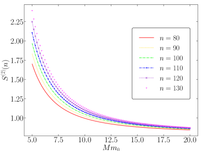
In Fig. 1 we depict the behaviour of the entropy in function of the dimensionless parameter . Since we have redefined the mass of the black hole as , we can observe that, for a fixed scalar-field mass, the matter contribution agrees with the generalized second law.
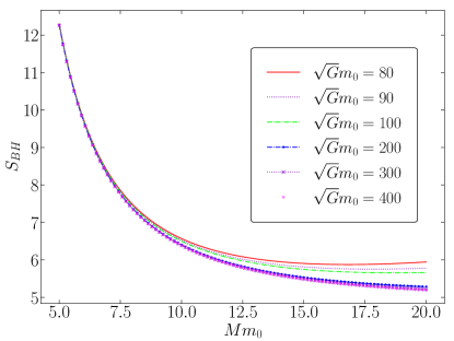
In Fig.2 we show the validity of the generalized second law of thermodynamics in black hole physics, where the total entropy of the system is the Bekenstein-Hawking entropy of the event horizon plus the contribution of the external matter fields correted by the influence of internal degrees of freedom defined inside the event horizon.
V Conclusions
We discussed, the limits of applicability of quantum field theory was put to the test by the formulation of quantum fields in curved spacetime. In this scenario, the concept of black hole entropy was introduced by Bekenstein. The concept of entropy can be formulated in many different ways. The thermodynamic or Boltzmann entropy which satisfies an additivity and non-decreasing condition which is related to observational states which are deterministic. By the other hand, the Gibbs entropy is defined in terms of ensembles. It is a function of the probabilities in a statistical ensemble. Both definitions are used for ordinary matter systems, i.e., usual thermodynamic systems. Since black holes are not such kind of systems, the literature has been emphasized that microscopic degrees of freedom are responsible for the Bekenstein-Hawking entropy. This idea of microscopic degrees of freedom of the internal configuration of the black hole have been used to discuss the definition of a statistical entropy. The total or generalized entropy of the black hole in four dimensions is given by the area of the event horizon , which is proportional to the Bekenstein-Hawking entropy of the system, and the contribution from the quantized matter. The first contribution is coming from the Euclidean action of the black hole instanton. Note that the usual way to compute the second contribution is that this quantity is the von Neumann entropy of the density matrix of the matter field outside the event horizon. This entanglement entropy across the boundary is ultraviolet divergent, that must be regularized and renormalized.
The constructive program claim that there is a unique formalism of quantum field theory and statistical mechanics of classical fields, given by probability theory. We discuss a quantum scalar field in the Euclidean section of the Schwarzschild manifold, i.e., a quantum field theory analytically continue to imaginary time. We use it to discussed a second contribution, defining the generalized entropy density of the black hole with contributions from external matter fields affected by the internal degrees of freedom inside the event horizon.
A conceptually simple way to model the influence of internal degrees of freedom over the matter fields, is to introduce a quenched disorder linearly coupled with the scalar field. To perform the integration over all the realizations of the disorder, we use the distributional zeta-function method. After integration over all the realizations of the disorder, we obtain a series representation of the averaged generating functional of connected correlation functions, in terms of the moments of the generating functional of correlation functions. Effective actions are defined for each of these moments. We show that this approach led us to the theory of Schrödinger operators in Riemannian manifolds. As far we known nowhere in the literature established this connection between the black hole thermodynamics and Schrödinger operators in Riemannian manifolds. The necessary and sufficient condition for essential self-adjointness of the generalized Schrödinger operator, constructed with the Laplace-Beltrami operator is discussed. If it is possible to define self-adjoint operators, the generating functional of connected correlation functions, can be defined. Finally, we present the generalized entropy density of the black hole with contributions from matter fields with the effective contribution of the internal degrees of freedom defined in the region inside the event horizon. We showed the validity of the generalized second law in the model here considered.
So far we have considered the influences of internal degrees of freedom over matter fields, modeled by an additive quenched disorder. One must consider also a multiplicative disorder situation [139]. As has been discussed in the literature, the main difference between the multiplicative and additive disorder, is that in the former, the effects of the disorder fluctuations does depend on the state of the system. This problem is under investigation by the authors.
Acknowledgments
The authors are grateful to S. A. Dias, B. F. Svaiter, A. M. S. Macedo, C. Farina, and G. Krein for fruitful discussions. This work was partially supported by Conselho Nacional de Desenvolvimento Científico e Tecnológico (CNPq), grant no. 305000/2023-3 (N.F.S.). G.S. thanks to Conselho Nacional de Desenvolvimento Científico e Tecnológico (CNPq) due the MSc. scholarship. G.O.H. thanks to Fundação Carlos Chagas Filho de Amparo à Pesquisa do Estado do Rio de Janeiro (FAPERJ) due the Ph.D. scholarship. C.D.R.C acknowledges the funding from the Engineering and Physical Sciences Research Council (EPSRC) (Grants No. EP/R513143/1 and No. EP/T517793/1).
References
- Rosenfeld [1965] L. Rosenfeld, Progress of Theoretical Physics Supplement E65, 222 (1965).
- Wheeler and Zurek [1983] J. A. Wheeler and W. H. Zurek, Quantum Theory and Measurement (Princeton University Press, New Jersey, USA, 1983).
- Lehmann et al. [1955] H. Lehmann, K. Symanzik, and W. Zimmermann, Nuovo Cimento 1, 205 (1955).
- Dyson [1952] F. J. Dyson, Phys. Rev. 85, 631 (1952).
- Petermann [1953] A. Petermann, Phys. Rev. 89, 1160 (1953).
- Svaiter [2005] N. Svaiter, Physica A 345, 517 (2005).
- Jaffe [1965] A. Jaffe, Comm. math. Phys. 1, 127 (1965).
- Landau et al. [1954a] L. D. Landau, A. A. Abrikosov, and I. M. Khalatnikov, Dokl. Akad. Nauk SSSR 95, 10.1016/b978-0-08-010586-4.50084-5 (1954a).
- Landau et al. [1954b] L. D. Landau, A. A. Abrikosov, and I. M. Khalatnikov, Dokl. Akad. Nauk SSSR 95, 1177 (1954b).
- Landau and Pomeranchuk [1955] L. D. Landau and I. Y. Pomeranchuk, Dokl. Akad. Nauk SSSR 102, 489 (1955).
- Wightman [1956] A. S. Wightman, Phys. Rev. 101, 860 (1956).
- Jaffe [1969] A. M. Jaffe, Rev. Mod. Phys. 41, 576 (1969).
- Streater [1975] R. F. Streater, Rep. Prog. Phys. 38, 771 (1975).
- Streater and Wightman [2000] R. Streater and A. Wightman, PCT, Spin and Statistics, and All that, Princeton landmarks in mathematics and physics (Princeton University Press, Princeton, USA, 2000).
- Symanzik [1964] K. Symanzik, A modified model of Euclidean quantum field theory, Tech. Rep. IMM-NYU 327 (New York University, Courant Institute of Mathematical Sciences, 1964).
- Guerra et al. [1975] F. Guerra, L. Rosen, and B. Simon, Ann. Math. 101, 111 (1975).
- Glimm and Jaffe [1981] J. Glimm and A. Jaffe, Quantum Physics A Functional Integral Point of View (Springer Verlag, New York, 1981).
- Jaffe [1985] A. Jaffe, Nucl. Phys. B 254, 31 (1985).
- Hilbert [1901] D. Hilbert, Archiv der Mathematik und Physik 3d (1901).
- Bohr and Rosenfeld [1933] N. Bohr and L. Rosenfeld, Mat. -fysiske Medd. 12 (1933).
- Bohr and Rosenfeld [1950] N. Bohr and L. Rosenfeld, Phys. Rev. 78, 794 (1950).
- Wigner [1939] E. P. Wigner, Ann. Math. 40, 149 (1939).
- Kolmogorov and Bharucha-Reid [2018] A. N. Kolmogorov and A. T. Bharucha-Reid, Foundations of the theory of probability (Dover, New York, USA, 2018).
- Kac [1959] M. Kac, Probability and Related Topics in Physical Sciences, Lectures in applied mathematics (American Mathematical Society) ; 1.A (Interscience Publishers, Providence, USA, 1959).
- Cramér [1999] H. Cramér, Mathematical Methods of Statistics (PMS-9) (Princeton University Press, Princeton, USA, 1999).
- Dyson [1949] F. J. Dyson, Phys. Rev. 75, 1736 (1949).
- Wick [1954] G. C. Wick, Phys. Rev. 96, 1124 (1954).
- Schwinger [1958] J. Schwinger, Proc. Natl. Acad. Sci. 44, 956 (1958).
- Nakano [1959] T. Nakano, Prog. Theo. Phys. 21, 241 (1959), https://academic.oup.com/ptp/article-pdf/21/2/241/5456644/21-2-241.pdf .
- Symanzik [1966] K. Symanzik, J. Math. Phys. 7, 510 (1966).
- Itô [1954] K. Itô, Memories of the College of Science, University Kyoto. Series A: Math. 28, 209 (1954).
- Yaglom [1957] A. M. Yaglom, Theory and Probability and its Applications 2, 273 (1957).
- Osterwalder and Schrader [1973] K. Osterwalder and R. Schrader, Comm. math. Phys. 31, 83 (1973).
- Osterwalder and Schrader [1975] K. Osterwalder and R. Schrader, Comm. math. Phys. 42, 281 (1975).
- Georgi [1993] H. Georgi, Annu. Rev. Nucl. Part. Sci. 43, 209 (1993).
- DeWitt [1975] B. S. DeWitt, Phys. Rep. 19, 295 (1975).
- Birrell and Davies [1982] N. D. Birrell and P. C. W. Davies, Quantum Fields in Curved Space, Cambridge Monographs on Mathematical Physics (Cambridge University Press, Cambridge, UK, 1982).
- Fulling [1989] S. A. Fulling, Aspects of quantum field theory in curved spacetime, 17 (Cambridge University Press, Cambridge, UK, 1989).
- Ford [1997] L. H. Ford, (1997), arXiv:gr-qc/9707062 [gr-qc] .
- Bekenstein [1972] J. D. Bekenstein, Lett. Nuovo Cimento 4, 737 (1972).
- Bekenstein [1973] J. D. Bekenstein, Phys. Rev. D 7, 2333 (1973).
- Hawking [1974] S. W. Hawking, Nature 248, 30 (1974).
- Hawking [1975] S. W. Hawking, Comm. math. Phys. 43, 199 (1975), [Erratum: Comm. math.Phys. 46, 206 (1976)].
- Davies [1978] P. C. Davies, Rep. Prog. Phys. 41, 1313 (1978).
- Kay and Wald [1991] B. S. Kay and R. M. Wald, Phys. Rep. 207, 49 (1991).
- Jacobson and Parentani [2003] T. Jacobson and R. Parentani, Found. of Phys. 33, 323 (2003).
- Hossenfelder and Smolin [2010] S. Hossenfelder and L. Smolin, Phys. Rev. D 81, 064009 (2010).
- Solodukhin [2011] S. N. Solodukhin, Living Rev. Relativity 14, 1 (2011).
- Carlip [2014] S. Carlip, Int. J. Mod. Phys. D 23, 1430023 (2014), arXiv:1410.1486 [gr-qc] .
- Hollands and Wald [2015] S. Hollands and R. M. Wald, Phys. Rep. 574, 1 (2015), arXiv:1401.2026 [gr-qc] .
- Harlow [2016] D. Harlow, Rev. Mod. Phys. 88, 015002 (2016), arXiv:1409.1231 [hep-th] .
- Raju [2022] S. Raju, Phys. Rep. 943, 1 (2022), arXiv:2012.05770 [hep-th] .
- Fronsdal [1959] C. Fronsdal, Phys. Rev. 116, 778 (1959).
- Kruskal [1960] M. D. Kruskal, Phys. Rev. 119, 1743 (1960).
- Hartle and Hawking [1976] J. B. Hartle and S. W. Hawking, Phys. Rev. D 13, 2188 (1976).
- Israel [1976] W. Israel, Phys. Lett. A 57, 107 (1976).
- Umezawa [1993] H. Umezawa, Advanced Field Theory: Micro, Macro, and Thermal Physics (American Inst. of Physics, New York, USA, 1993).
- Srinivasan and Padmanabhan [1999] K. Srinivasan and T. Padmanabhan, Phys. Rev. D 60, 024007 (1999), arXiv:gr-qc/9812028 .
- Parikh and Wilczek [2000] M. K. Parikh and F. Wilczek, Phys. Rev. Lett. 85, 5042 (2000).
- Fredenhagen and Haag [1990] K. Fredenhagen and R. Haag, Comm. math. Phys. 127, 273 (1990).
- Sewell [1980] G. L. Sewell, Phys. Lett. A 79, 23 (1980).
- Sewell [1982] G. L. Sewell, Ann. Phys. 141, 201 (1982).
- Fulling and Ruijsenaars [1987] S. Fulling and S. Ruijsenaars, Phys. Rep. 152, 135 (1987).
- Kubo [1957] R. Kubo, J. Phys. Japan 12, 570 (1957).
- Martin and Schwinger [1959] P. C. Martin and J. S. Schwinger, Phys. Rev. 115, 1342 (1959).
- Gârding and Wightman [1954] L. Gârding and A. Wightman, Proc. Nat. Acad. Sci. 40, 617 (1954), https://www.pnas.org/doi/pdf/10.1073/pnas.40.7.617 .
- Wightman and Schweber [1955] A. S. Wightman and S. S. Schweber, Phys. Rev. 98, 812 (1955).
- Fulling [1973] S. A. Fulling, Phys. Rev. D 7, 2850 (1973).
- Unruh [1976] W. G. Unruh, Phys. Rev. D 14, 870 (1976).
- Davies [1975] P. C. W. Davies, J. Phys. A 8, 609 (1975).
- Sciama et al. [1981] D. W. Sciama, P. Candelas, and D. Deutsch, Adv. Phys. 30, 327 (1981).
- Takagi [1986] S. Takagi, Prog. Theor. Phys. 88, 1 (1986).
- Svaiter and Svaiter [1992] B. F. Svaiter and N. F. Svaiter, Phys. Rev. D 46, 5267 (1992).
- Soares et al. [2021] M. S. Soares, N. F. Svaiter, C. A. D. Zarro, and G. Menezes, Phys. Rev. A 103, 042225 (2021), arXiv:2009.03970 [hep-th] .
- Christensen and Duff [1978] S. M. Christensen and M. J. Duff, Nucl. Phys. B 146, 11 (1978).
- Svaiter and Zarro [2008] N. F. Svaiter and C. A. D. Zarro, Class. Quant. Grav. 25, 095008 (2008).
- Hiscock et al. [1997] W. A. Hiscock, S. L. Larson, and P. R. Anderson, Phys. Rev. D 56, 3571 (1997).
- Gelfand and Yaglom [1960] I. M. Gelfand and A. M. Yaglom, J. Math. Phys. 1, 48 (1960).
- Fradkin [1963] E. S. Fradkin, Nucl. Phys. 49, 624 (1963).
- York [1983] J. W. York, Jr., Phys. Rev. D 28, 2929 (1983).
- Frolov and Novikov [1993] V. P. Frolov and I. Novikov, Phys. Rev. D 48, 4545 (1993), arXiv:gr-qc/9309001 .
- Barvinsky et al. [1995] A. O. Barvinsky, V. P. Frolov, and A. I. Zelnikov, Phys. Rev. D 51, 1741 (1995), arXiv:gr-qc/9404036 .
- Frolov and Fursaev [1998] V. P. Frolov and D. V. Fursaev, Class. Quant. Grav. 15, 2041 (1998), arXiv:hep-th/9802010 .
- Bekenstein [1974] J. D. Bekenstein, Phys. Rev. D 9, 3292 (1974).
- Wald [1979] R. M. Wald, Comm. math. Phys. 70, 221 (1979).
- Haag et al. [1984] R. Haag, H. Narnhofer, and U. Stein, Comm. math. Phys. 94, 219 (1984).
- Jaffe and Ritter [2007] A. Jaffe and G. Ritter, Comm. math. Phys. 270, 545 (2007), arXiv:hep-th/0609003 .
- Bombelli et al. [1986] L. Bombelli, R. K. Koul, J. Lee, and R. D. Sorkin, Phys. Rev. D 34, 373 (1986).
- Callan and Wilczek [1994] C. G. Callan, Jr. and F. Wilczek, Phys. Lett. B 333, 55 (1994), arXiv:hep-th/9401072 .
- Kabat [1995] D. N. Kabat, Nucl. Phys. B 453, 281 (1995), arXiv:hep-th/9503016 .
- Terashima [2000] H. Terashima, Phys. Rev. D 61, 104016 (2000), arXiv:gr-qc/9911091 .
- Das et al. [2008] S. Das, S. Shankaranarayanan, and S. Sur, Phys. Rev. D 77, 064013 (2008), arXiv:0705.2070 [gr-qc] .
- Brout [1959] R. Brout, Phys. Rev. 115, 824 (1959).
- Klein and Brout [1963] M. W. Klein and R. Brout, Phys. Rev. 132, 2412 (1963).
- Svaiter and Svaiter [2016a] B. F. Svaiter and N. F. Svaiter, Int. J. Mod. Phys. A 31, 1650144 (2016a), arXiv:1603.05919 [cond-mat.stat-mech] .
- Svaiter and Svaiter [2016b] B. F. Svaiter and N. F. Svaiter, Disordered field theory in and distributional zeta-function (2016b), arXiv:1606.04854 [math-ph] .
- Acosta Diaz et al. [2020] R. J. Acosta Diaz, C. D. Rodríguez-Camargo, and N. F. Svaiter, Polymers 12, 10.3390/polym12051066 (2020).
- Shubin [1992] M. A. Shubin, Astérisque 207, 35 (1992).
- Braverman et al. [2002] M. Braverman, O. Milatovic, and M. Shubin, Russian. Math. Survays 57, 641 (2002).
- Sorkin [1986] R. D. Sorkin, Phys. Rev. Lett. 56, 1885 (1986).
- Wall [2012] A. C. Wall, Phys. Rev. D 85, 104049 (2012), [Erratum: Phys.Rev.D 87, 069904 (2013)], arXiv:1105.3445 [gr-qc] .
- Myers and Perry [1986] R. C. Myers and M. J. Perry, Ann. Phys. 172, 304 (1986).
- Kadanoff and Baym [1989] L. P. Kadanoff and G. Baym, Perseus Books (Cambridge, Massachusetts, 1989).
- Landsman and van Weert [1987] N. P. Landsman and C. G. van Weert, Phys. Rep. 145, 141 (1987).
- Symanzik [1981] K. Symanzik, Nucl. Phys. B 190, 1 (1981).
- Diehl and Dietrich [1981] H. W. Diehl and S. Dietrich, Phys. Rev. B 24, 2878 (1981).
- Fosco and Svaiter [2001] C. D. Fosco and N. F. Svaiter, J. Math. Phys. 42, 5185 (2001), arXiv:hep-th/9910068 .
- Caicedo and Svaiter [2004] M. I. Caicedo and N. F. Svaiter, J. Math. Phys. 45, 179 (2004), arXiv:hep-th/0207202 .
- Svaiter [2004] N. F. Svaiter, J. Math. Phys. 45, 4524 (2004), arXiv:hep-th/0410016 .
- Aparicio Alcalde et al. [2006] M. Aparicio Alcalde, G. Flores Hidalgo, and N. F. Svaiter, J. Math. Phys. 47, 052303 (2006), arXiv:hep-th/0512100 .
- Gibbons and Perry [1976] G. W. Gibbons and M. J. Perry, Phys. Rev. Lett. 36, 985 (1976).
- Rivers [1988] R. J. Rivers, Path integral methods in quantum field theory (Cambridge University Press, Cambridge, UK, 1988).
- Zinn-Justin [2021] J. Zinn-Justin, Quantum field theory and critical phenomena, Vol. 171 (Oxford University Press, Oxford, UK, 2021).
- Matyjasek [2018] J. Matyjasek, Phys. Rev. D 98, 104054 (2018), arXiv:1811.00993 [gr-qc] .
- Arcuri et al. [1994] R. C. Arcuri, N. F. Svaiter, and B. F. Svaiter, Mod. Phys. Lett. A 9, 19 (1994).
- Edwards and Anderson [1975] S. F. Edwards and P. W. Anderson, J. Phys. F 5, 965 (1975).
- Emery [1975] V. J. Emery, Phys. Rev. B 11, 239 (1975).
- Mézard et al. [1987] M. Mézard, G. Parisi, and M. A. Virasoro, Spin glass theory and beyond: An Introduction to the Replica Method and Its Applications, Vol. 9 (World Scientific Publishing Company, Singapore, 1987).
- Dotsenko [2005] V. Dotsenko, Introduction to the Replica Theory of Disordered Statistical Systems (2005).
- De Dominicis [1978] C. De Dominicis, Phys. Rev. B 18, 4913 (1978).
- Sompolinsky and Zippelius [1981] H. Sompolinsky and A. Zippelius, Phys. Rev. Lett. 47, 359 (1981).
- De Dominicis and Giardina [2006] C. De Dominicis and I. Giardina, Random fields and spin glasses: a field theory approach (Cambridge University Press, Cambridge, UK, 2006).
- Efetov [1983] K. B. Efetov, Adv. Phys. 32, 53 (1983).
- Abramowitz and Stegun [1965] M. Abramowitz and I. Stegun, Handbook of Mathematical Functions: With Formulas, Graphs, and Mathematical Tables, Applied mathematics series (Courier Corporation, Massachusetts, USA, 1965).
- Rodríguez-Camargo et al. [2022] C. D. Rodríguez-Camargo, A. Saldivar, and N. F. Svaiter, Phys. Rev. D 105, 105014 (2022), arXiv:2108.02330 [cond-mat.dis-nn] .
- Heymans et al. [2024] G. O. Heymans, N. F. Svaiter, B. F. Svaiter, and G. Krein, Critical Casimir effect in a disordered -symmetric model (2024), arXiv:2402.01588 [cond-mat.soft] .
- Diaz et al. [2017] R. A. Diaz, G. Menezes, N. F. Svaiter, and C. A. D. Zarro, Phys. Rev. D 96, 065012 (2017), arXiv:1705.06403 [hep-th] .
- Diaz et al. [2018] R. A. Diaz, G. Krein, N. F. Svaiter, and C. A. D. Zarro, Phys. Rev. D 97, 065017 (2018), arXiv:1712.07990 [cond-mat.stat-mech] .
- Rodríguez-Camargo et al. [2021] C. D. Rodríguez-Camargo, E. A. Mojica-Nava, and N. F. Svaiter, Phys. Rev. E 104, 034102 (2021), arXiv:2102.11977 [cond-mat.dis-nn] .
- Heymans et al. [2022] G. O. Heymans, N. F. Svaiter, and G. Krein, Phys. Rev. D 106, 125004 (2022), arXiv:2207.06927 [hep-th] .
- Heymans et al. [2023] G. O. Heymans, N. F. Svaiter, and G. Krein, Int. J. Mod. Phys. D 32, 2342019 (2023), arXiv:2305.07990 [hep-th] .
- Kato [1973] T. Kato, Israel J. of Math. 13, 10.1007/BF02760233 (1973).
- Lieb [1976] E. Lieb, Bull. Amer. Math. Soc. 82, 751 (1976).
- Davies [2002] E. B. Davies, Bull. London Math. Soc. 34, 513 (2002).
- Diyab and Reddy [2022] F. Diyab and B. S. Reddy, Comm. math. Applic. 13, 1475 (2022).
- Olejnik [1993] I. M. Olejnik, Math. Notes 54, 934 (1993).
- Bardeen et al. [1973] J. M. Bardeen, B. Carter, and S. W. Hawking, Comm. math. Phys. 31, 161 (1973).
- Robinson and Ruelle [1967] D. W. Robinson and D. Ruelle, Comm. math. Phys. 5, 288 (1967).
- Soares et al. [2020] M. S. Soares, N. F. Svaiter, and C. A. D. Zarro, Class. Quant. Grav. 37, 065024 (2020).