Nonlinear chiral quantum optics with giant-emitter pairs
Xin Wang
wangxin.phy@xjtu.edu.cnInstitute of Theoretical Physics, School of Physics, Xi’an
Jiaotong University, Xi’an 710049, People’s Republic of China
Theoretical Quantum Physics Laboratory, RIKEN Cluster for
Pioneering Research, Wako-shi, Saitama 351-0198, Japan
Jia-Qi Li
Institute of Theoretical Physics, School of Physics, Xi’an
Jiaotong University, Xi’an 710049, People’s Republic of China
Zhihai Wang
Center for Quantum Sciences and School of Physics, Northeast
Normal University, Changchun 130024, People’s Republic of China
Anton Frisk Kockum
Department of Microtechnology and Nanoscience, Chalmers
University of Technology, 41296 Gothenburg, Sweden
Lei Du
Department of Microtechnology and Nanoscience, Chalmers
University of Technology, 41296 Gothenburg, Sweden
Tao Liu
liutao0716@scut.edu.cnSchool of Physics and Optoelectronics, South China University of
Technology, Guangzhou 510640, People’s Republic of China
Franco Nori
Theoretical Quantum Physics Laboratory, RIKEN Cluster for
Pioneering Research, Wako-shi, Saitama 351-0198, Japan
Center for Quantum Computing, RIKEN, Wako-shi, Saitama 351-0198,
Japan
Physics Department, The University of Michigan, Ann Arbor,
Michigan 48109-1040, USA
Abstract
We propose a setup which combines giant emitters (coupling to light at
multiple points separated by wavelength distances) with nonlinear quantum
optics and its correlated photons. In this setup, we reveal a mechanism
for multiphoton chiral emission: the propagation phase of the center of
mass of two strongly correlated photons (a doublon), and the phases
encoded in the coupling points of two giant emitters, can yield
completely destructive interference in one propagation direction while
supporting emission in the other direction. The degree of chirality can
be tuned by the phases of the couplings.
We show that the proposed setup can provide directional quantum many-body
resources, and can be configured as a building block for a chiral quantum
network with “correlated flying qubits”, enabling distinct applications
beyond linear chiral setups. Our findings point toward a rich landscape
of tailoring multiphoton propagation and correlation properties by
exploiting interference effects of giant emitters coupling to nonlinear
photonic baths.
Introduction.—Chiral quantum optics, where photons can be routed
without information backflow, is a prerequisite for communication protocols
in a scalable quantum network [1, 2, 3, 4, 5, 6, 7, 8, 9, 10]. Directional photons (serving as flying qubits) can connect
remote nodes deterministically and underpin unique applications beyond
conventional bidirectional networks [11, 12, 13, 14, 15, 16, 17, 18, 19, 20, 21]. Recently, the nonlinear
(multiphoton) regime of chiral quantum optics, which can provide directional
many-body resources in quantum communication, metrology, and
sensing [22, 23, 24, 25, 26], has yielded many interesting proposals [27, 28, 29, 30, 31, 32, 33]. For example, due to the interplay of nonlinearity and chiral
transport, many-body ordered states of light can be produced in a
waveguide [34]. However, in conventional optical materials,
the nonlinearity is ultraweak [35, 36] and the
unidirectional photons are usually uncorrelated. Reaching the nonlinear
regime of chiral quantum optics is therefore challenging and so far less
studied.
Meanwhile, another recently introduced paradigm of quantum optics, giant
atoms, has attracted growing interest [37, 38, 39, 40, 41, 42, 43, 44, 45, 46, 47, 48, 49]. The size of a giant atom is
comparable to the wavelength of the photons it interacts with; this relation
can be realized by having multiple coupling points with photonic (or
phononic) baths [38, 39, 50, 51, 52, 53, 54, 55, 56, 40, 57, 58, 59, 60, 61, 62, 63, 64, 65]. The interference [38, 60] and time-retardation [51, 54] effects due
to the multiple coupling points of giant atoms can lead to exotic quantum
phenomena such as dipole-dipole interactions free of
decoherence [66, 40, 57, 44, 46, 67], oscillating bound states [59, 56, 48, 68, 69], and chiral quantum
phenomena [55, 42, 70, 62, 65, 71]. However, most studies on giant atoms consider linear quantum
optics, where photons are usually uncorrelated.
In this Letter, we merge these two fields by considering giant-emitter pairs
interacting with nonlinear waveguides. In this setup, we find a mechanism for
chiral emission of strongly correlated photons. Unlike conventional
single-photon chiral setups, our proposal can be a building block for a
nonlinear cascaded quantum network mediated by “correlated flying qubits”,
which can be encoded with information to manipulate many-body states of
remote nodes.
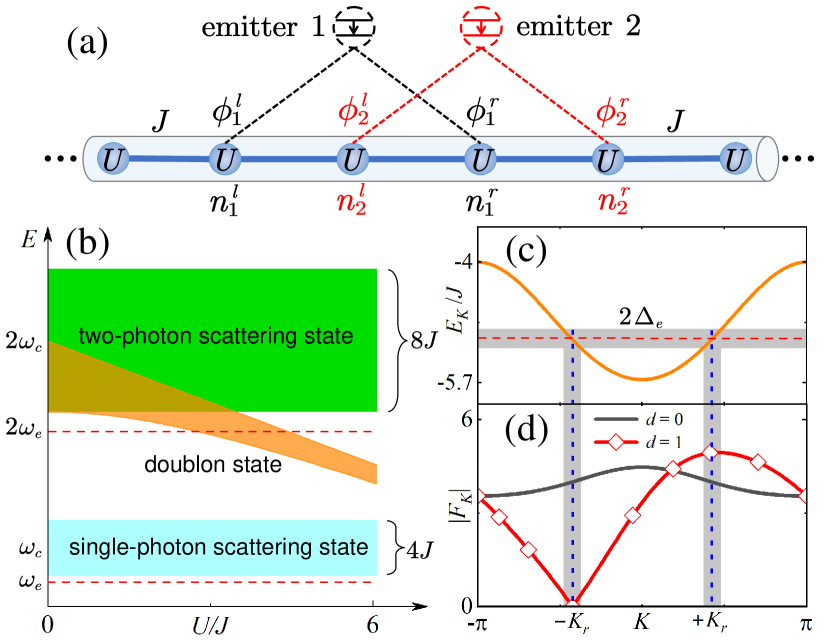
Figure 1: (a) Sketch of a giant-emitter pair (GEP) coupled to a nonlinear
waveguide (a coupled-cavity array with hopping rates and on-site
nonlinear potentials ). Giant emitter couples to the waveguide at
with phases . The emitter size is ; the emitter centers are separated by a distance .
(b) Waveguide spectrum as a function of . The upper (lower) red
dashed line marks the GEP (single emitter) frequency
().
(c) Doublon dispersion relation .
(d) Effective coupling strength as a function of doublon wave
vector for different . When , is the optimal
chiral point.
Parameters: , , and .
Model—The nonlinear waveguide in our setup consists of an array of
coupled nonlinear cavities, as depicted in Fig. 1(a). In the frame
rotating with the cavity frequency , the waveguide Hamiltonian is
()
(1)
where () is the photon annihilation (creation) operator of
the th cavity, is the nearest-neighbor hopping rate, and is the
on-site photon-photon interaction strength. Due to the nonlinear potential, a
photonic state called “doublon” [72, 73, 74, 75, 76, 77, 78, 79, 80, 81, 82], where two photons are bound
together when propagating along the waveguide, emerges in the two-photon
subspace. The dispersion relation of the doublon state with wave vector
is [see Fig. 1(c)]. The
corresponding eigenwavefunction is , where
exponentially decays with the distance
between the two photons (at and ) and
is the center-of-mass coordinate. A detailed derivation is provided in Sec. I
in the Supplemental Material [83].
We now consider a giant-emitter pair (GEP) interacting with the waveguide.
The two coupling points of emitter are located at [; see Fig. 1(a)]. The full system Hamiltonian is
(2)
with ( is the emitter frequency),
the coupling strength at each coupling point, a Pauli matrix,
and the lowering operator. A local phase is
assumed at each coupling point. The size of emitter is and the distance between the centers of the two emitters is . When is significantly
gapped from scattering states, i.e., , emission of a single
photons is suppressed. We set lying inside the doublon spectrum
[see Fig. 1(b)] such that the GEP will emit correlated photons,
i.e., doublons [80].
We assume that, initially, the two emitters are in their excited states and
the waveguide is in its vacuum state. Since the Hamiltonian in Eq. (2)
conserves the total excitation number, the system state is
(3)
where [] is the probability amplitude for the GEP (doublon
mode ) being excited, is the creation operator of
doublon mode , are the
photonic operators in momentum space, and is the probability for
both the th giant emitter and the single-photon mode being
excited. Given that , we can adiabatically
eliminate the single-photon intermediate states by assuming
. The evolution of and is then given
by [83]
(4)
(5)
(6)
where is a summation of correlation functions of different coupling
points:
(7)
with . The amplitude of is with .
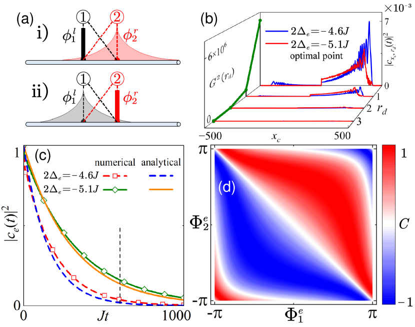
Figure 2: (a) Sketches of the dual transition processes described by .
(b) The two-photon field distributions at [dashed line in
(c)].
The two-point correlation function is plotted for (optimal point). (c) Evolution of for .
(d) Chiral factor as a function of and . The
coupling strength is set to ; other parameters are the
same as in Fig. 1(d).
Taking schematically depicted in
Fig. 2(a) as an example, we see that this correlation function
represents dual processes: emitter 1 (2) excites a single-photon
intermediate state spreading around the point () with an
encoded phase (). Meanwhile, emitter 2 (1) emits a
single photon at point () with encoded phase
(). The overlap between the wave functions of these photon pairs
and the doublon state is proportional to (cf. Sec. II in Ref. [83]).
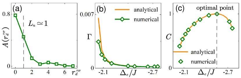
Interference-induced supercorrelated chiral emission—We assume
that the effective coupling strength is sufficiently weak
compared to the doublon bandwidth that the Born–Markov approximation
holds [84]. The supercorrelated decay of the GEP then becomes
(8)
where , is the group velocity, and ()
denotes the supercorrelated emission rate to the right (left). These rates
define the chiral factor . In Ref. [83], we prove that only the
relative coupling phases of each emitter, i.e., , affect the dynamics.
Setting , , and , we plot the waveguide
field distribution and the evolution of in
Fig. 2(b)-(c). The numerically calculated evolution is an
exponential decay, in excellent agreement with analytical results. Due to the
local nonlinear potential, the two photons are strongly bunched; the spatial
correlation function has its maximum at . Most
strikingly, the emission of this correlated photon pair exhibits a strong
chiral preference, as shown in Fig. 2(b).
Increasing (fixing ), the chiral factor changes little, while the
decay rate quickly decreases to zero [83]. The ordering of the
coupling points, crucial in Ref. [66], has no significant effect
on the chiral dynamics. Details on the effect of varying and are
given in Ref. [83]. Figure 2(d) plots
as a function of the phases , showing that strong chirality
is robust to relatively large imprecision in and that can
be smoothly tuned in the full range by changing
. These key results indicate that the proposed setup may serve
well as a source for directional correlated photons.
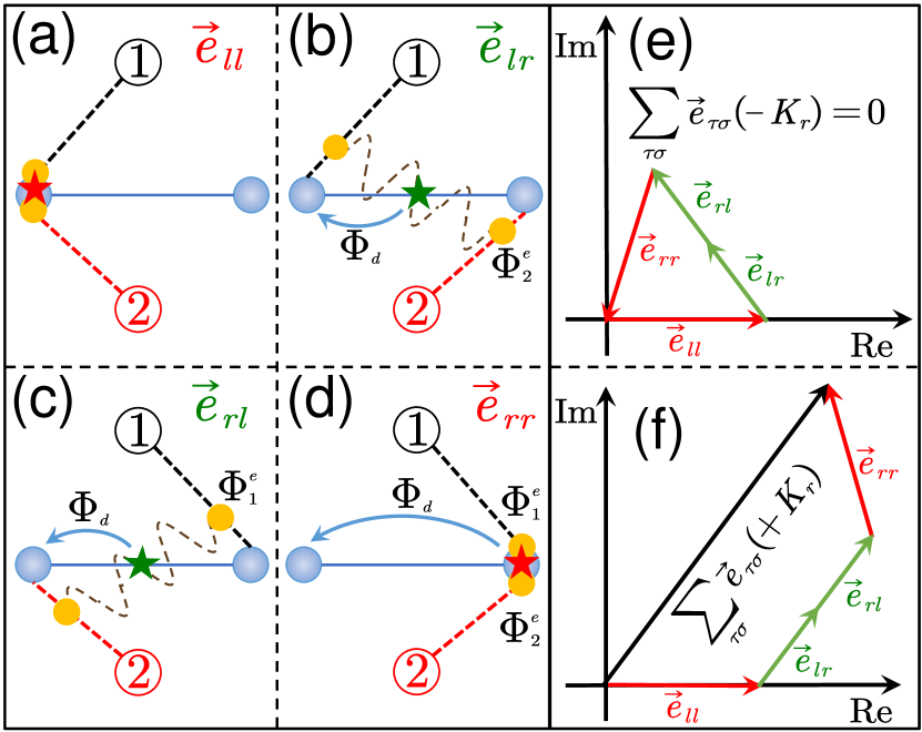
Figure 3: (a–d) Sketches of the four decay channels () of a GEP releasing two correlated
photons into the waveguide. Orange dots represent single photons emitted
from individual emitters, while stars denote centers of mass of the
correlated photon pairs.
(e, f) Summation of at the optimal point for right- (left-) propagating modes.
To better understand the mechanism for chirality, we depict the four
supercorrelated decay channels in Fig. 3(a)-(d), with orange dots
denoting single photons emitted from distinct emitters and stars centers of
mass of correlated photon pairs. We represent
as four vectors in complex space. The phase of
consists of the local phases and the accumulated propagation phase associated with the center of mass of
the correlated photon pair (not the single-photon propagation phase).
Therefore , which corresponds
to interference between these channels. With as the
reference point, the propagation phases for the channels are , , and .
Figure 1(d) shows as a function of for
different . When , the emitters are small and
always, regardless of , so there is no chiral emission.
However, for giant emitters with , chiral emission of correlated
photon pairs emerges when . As shown in
Fig. 3(e)-(f), at the optimal point , the
interferences for the left- and right-propagating modes become asymmetric:
the four vectors for form a closed loop, i.e.,
.
The interaction between the GEP and the left-propagating mode vanishes [see
Fig. 1(d)] and the GEP only emits correlated photons into the right
direction, yielding . When is biased away from the
optimal point, decreases, as indicated in Fig. 2(b).
Note that our examples are the simplest giant emitters with two coupling
points. For GEPs with coupling points per emitter, there are
supercorrelated decay channels interfering with each other,
which is much more complicated than single-photon interference in one giant
atom [38, 85, 63]. When , it is
possible to realize broadband chiral emission for doublons by considering the
optimal methods in Ref. [71], which could be addressed in future
work.
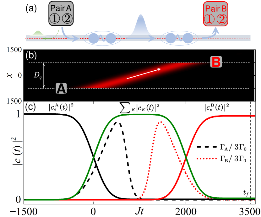
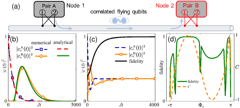
Figure 4: (a) Sketch of the nonlinear cascaded quantum system, where
correlated photon pairs are unidirectionally emitted by GEP A and
subsequently absorbed by GEP B without back-scattering.
(b) The evolution of two-photon field distribution at and
(c) populations for the GEPs and a doublon during the two-photon
transfer process. The dashed lines in (b) mark the positions of GEP A
and B, which are separated by a distance . The
modulations of the couplings are given by Eq. (10). Same
parameters as in Fig. 2.
Chiral quantum network with correlated photons—Our proposal can be
extended into a chiral quantum network where propagating photon pairs are
unidirectionally transferred without information backflow. In contrast to
standard setups with single flying qubits, more quantum information can be
encoded into “correlated flying qubits”. Figure 4(a)
depicts a minimal example setup with two separate GEPs, A and B, interacting
with a common waveguide. The interaction Hamiltonian is
approximately [83]
(9)
where is the
joint-quantum-jump operator for GEP with the
lowering operator of emitter and the correlation
functions of GEP [see Eq. (6)]. The collective and individual
supercorrelated decay rates for the two GEPs are (), where () represents propagation to the right
(left) [83]. Given that each GEP couples chirally to the
waveguide with , a
photon pair can be unidirectionally radiated by GEP A and subsequently
absorbed by the GEP B without back-scattering. In Ref. [83], we
derive the master equation for this cascaded quantum system with
joint-quantum-jump processes under the Markovian approximation.
Many applications in linear cascaded quantum networks [12, 13, 14] can find their nonlinear counterparts in GEPs
connected by doublons. Moreover, the correlated flying qubits can enhance
numerous applications which are not accounted for in a linear chiral
interface, e.g., manipulating many-body quantum states involving remote
nodes. Such many-body states are essential to quantum-enhanced metrology and
quantum simulations [23, 24, 25, 26]. By applying strong coherent drives to two remote GEPs, we show
that those emitters can be trapped in stationary four-partite entangled
states [83]. Below, we demonstrate another intriguing process
for high-fidelity entangled-state transfer: maintaining dark-state conditions
with time-dependent decay rates. Contrasting single-qubit state transfer in
linear chiral systems [1, 14, 17, 18], our proposal enables high-fidelity entangled-state transfer
between remote GEPs.
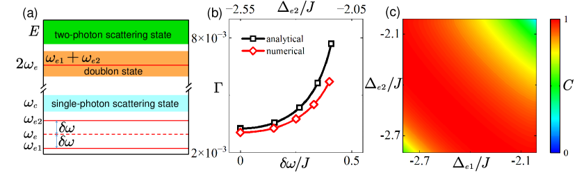
We assume that the decay rates for two GEPs [separated with a distance ;
see Fig. 4(b)] undergo the following
modulation [13, 65]:
(10)
where with the decay rate of
GEP A at , and is the propagation time from A to
B. The modulating pulses in Eq. (10) minimize irreversible quantum jump
processes and tailor the wavepacket of the correlated photons with
time-reversal symmetry. Therefore, GEP B will perfectly absorb two correlated
photons emitted by GEP A [13]. Because in our proposal [cf. Eq. (S48)], the
modulated decay rates can be exactly mapped to time-dependent interactions
. We numerically simulate two-excitation transfer
between two GEPs in Fig. 4(b)-(c). Because dark-state conditions
always hold in this nonlinear cascaded system, the correlated-two-photon
field is trapped between the two GEPs without leaking outside. At the final
time , one finds that . The absorption efficiency is [83], which enables a high-fidelity
entangled-state transfer between two remote GEPs given that the initial state
of GEP A is . In Ref. [83], we show that, by reversing the signs of
and instead of modulating the couplings, the proposed setup can be
engineered as a nonlinear phase-conjugate mirror for
doublons [86, 87], which also can be employed for
high-fidelity entangled-state transfer processes.
Conclusion—We show how to realize unidirectional transport of
strongly correlated photons in a nonlinear waveguide interacting with
giant-emitter pairs. Compared to the single-photon case, the interference
channels are more complicated, and the propagating phase related to the
center of mass of the correlated photons plays an important role in
interference between those channels. Another key ingredient, the local
coupling phases of GEPs, does not only lead to asymmetric interference
relations for oppositely propagating modes, but also provides the necessary
degree of freedom for tuning the chiral directions. Our setup can potentially
be implemented as a building block for a chiral quantum network with
“correlated flying qubits”, which underpins unique applications beyond
linear chiral setups.
Our proposal is feasible in circuit-QED systems [88, 89, 90], where giant emitters have been implemented in
experiments [40, 60, 65]. An array of coupled
transmon qubits [91], extensively studied in Refs. [92, 93, 94, 95], can be configured as the nonlinear
waveguide. Time-dependent interactions between superconducting giant atoms
and the waveguide can be realized with the methods in
Ref. [65]. Our work demonstrates a striking example of how
correlated emission is significantly modified by the interplay of giant atoms
and the nonlinearity of a bath, which might inspire future studies with
correlated photons beyond pairs, e.g., “trions” [96]. We believe
it offers interesting new perspectives for harnessing many-body states and
provides a powerful toolbox for large-scale quantum information processing.
Acknowledgments.
The numerical simulations of quantum dynamics are based on the
open-source Python package QuTiP [97, 98].
X.W. is supported by the National Natural Science Foundation of China
(NSFC) (Grant No. 12174303).
Z.H.W. acknowledges the support from National Natural Science Foundation
of China (Grant No. 12375010).
T.L. acknowledges the support from National Natural Science Foundation of
China (Grant No. 12274142), the Startup Grant of South China University
of Technology (Grant No. 20210012) and Introduced Innovative Team Project
of Guangdong Pearl
River Talents Program (Grant No. 2021ZT09Z109).
A.F.K. acknowledges support from the Swedish Research Council (grant
number 2019-03696), the Swedish Foundation for Strategic Research (grants
numbers FFL21-0279 and FUS21-0063), the Horizon Europe programme
HORIZON-CL4-2022-QUANTUM-01-SGA via the project 101113946
OpenSuperQPlus100, and from the Knut and Alice Wallenberg Foundation
through the Wallenberg Centre for Quantum Technology (WACQT).
F.N. is supported in part by: Nippon Telegraph and Telephone Corporation
(NTT) Research, the Japan Science and Technology Agency (JST) [via the
Quantum Leap Flagship Program (Q-LEAP), and the Moonshot R&D Grant
Number JPMJMS2061], the Asian Office of Aerospace Research and
Development (AOARD) (via Grant No. FA2386-20-1-4069), and the Office of
Naval Research (ONR) (via Grant No. N62909-23-1-2074).
References
Cirac et al. [1997]J. I. Cirac, P. Zoller,
H. J. Kimble, and H. Mabuchi, Quantum State Transfer and Entanglement
Distribution among Distant Nodes in a Quantum Network, Phys. Rev. Lett. 78, 3221 (1997).
Mitsch et al. [2014]R. Mitsch, C. Sayrin,
B. Albrecht,
P. Schneeweiss, and A. Rauschenbeutel, Quantum state-controlled directional
spontaneous
emission of photons into a nanophotonic waveguide, Nature Communications 5, 5713 (2014).
Pichler et al. [2015]H. Pichler, T. Ramos,
A. J. Daley, and P. Zoller, Quantum optics of chiral spin networks, Phys. Rev. A 91, 042116 (2015).
Bliokh and Nori [2015]K. Y. Bliokh and F. Nori, Transverse and longitudinal angular
momenta of light, Phys. Rep. 592, 1 (2015).
Söllner et al. [2015]I. Söllner, S. Mahmoodian, S. L. Hansen, L. Midolo,
A. Javadi, G. Kirsanske, T. Pregnolato, H. El-Ella, E. H. Lee, J. D. Song, S. Stobbe, and P. Lodahl, Deterministic
photon-emitter coupling in chiral photonic circuits, Nature Nanotechnology 10, 775 (2015).
Lodahl et al. [2017]P. Lodahl, S. Mahmoodian,
S. Stobbe, A. Rauschenbeutel, P. Schneeweiss, J. Volz, H. Pichler, and P. Zoller, Chiral
quantum optics, Nature 541, 473 (2017).
Barik et al. [2018]S. Barik, A. Karasahin,
C. Flower, T. Cai, H. Miyake, W. DeGottardi, M. Hafezi, and E. Waks, A
topological quantum optics interface, Science 359, 666 (2018).
Ozawa et al. [2019]T. Ozawa, H. M. Price,
A. Amo, N. Goldman, M. Hafezi, L. Lu, M. C. Rechtsman, D. Schuster, J. Simon,
O. Zilberberg, and I. Carusotto, Topological photonics, Rev. Mod. Phys. 91, 015006 (2019).
De Bernardis et al. [2023]D. De Bernardis, F. S. Piccioli, P. Rabl, and I. Carusotto, Chiral Quantum Optics in the Bulk
of
Photonic Quantum Hall Systems, PRX Quantum 4, 030306 (2023).
Maffei et al. [2024]M. Maffei, D. Pomarico,
P. Facchi, G. Magnifico, S. Pascazio, and F. Pepe, Directional emission and photon bunching from a qubit pair in
waveguide, arXiv:2402.01286 (2024).
Stannigel et al. [2010]K. Stannigel, P. Rabl,
A. S. Sørensen,
P. Zoller, and M. D. Lukin, Optomechanical Transducers for Long-Distance Quantum
Communication, Phys. Rev. Lett. 105, 220501 (2010).
Stannigel et al. [2011]K. Stannigel, P. Rabl,
A. S. Sørensen,
M. D. Lukin, and P. Zoller, Optomechanical transducers for
quantum-information
processing, Phys. Rev. A 84, 042341 (2011).
Stannigel et al. [2012]K. Stannigel, P. Rabl, and P. Zoller, Driven-dissipative preparation of
entangled states in cascaded quantum-optical networks, New Journal of Physics 14, 063014 (2012).
Northup and Blatt [2014]T. E. Northup and R. Blatt, Quantum
information
transfer using photons, Nature Photonics 8, 356 (2014).
Mahmoodian et al. [2016]S. Mahmoodian, P. Lodahl, and A. S. Sørensen, Quantum Networks with
Chiral-Light–Matter Interaction in Waveguides, Phys. Rev. Lett. 117, 240501 (2016).
Vermersch et al. [2017]B. Vermersch, P.-O. Guimond, H. Pichler, and P. Zoller, Quantum State Transfer via Noisy
Photonic and Phononic Waveguides, Phys. Rev. Lett. 118, 133601 (2017).
Xiang et al. [2017]Z.-L. Xiang, M. Zhang,
L. Jiang, and P. Rabl, Intracity Quantum Communication via Thermal Microwave
Networks, Phys. Rev. X 7, 011035 (2017).
Calajó et al. [2019]G. Calajó, M. J. A. Schuetz, H. Pichler,
M. D. Lukin,
P. Schneeweiss, J. Volz, and P. Rabl, Quantum acousto-optic control of light-matter interactions in
nanophotonic networks, Phys. Rev. A 99, 053852 (2019).
Guimond et al. [2020]P.-O. Guimond, B. Vermersch,
M. L. Juan,
A. Sharafiev, G. Kirchmair, and P. Zoller, A unidirectional on-chip photonic interface for
superconducting
circuits, npj Quantum Information 6, 32 (2020).
Kannan et al. [2023]B. Kannan, A. Almanakly,
Y. Sung, A. Di Paolo, D. A. Rower, J. Braumüller, A. Melville, B. M. Niedzielski, A. Karamlou, K. Serniak, A. Vepsäläinen, M. E. Schwartz, J. L. Yoder, R. Winik, J. I.-J. Wang,
T. P. Orlando,
S. Gustavsson, J. A. Grover, and W. D. Oliver, On-demand directional microwave photon emission using
waveguide quantum electrodynamics, Nature Physics 19, 394 (2023).
Imoto et al. [1985]N. Imoto, H. A. Haus, and Y. Yamamoto, Quantum nondemolition measurement
of
the photon number via the optical Kerr effect, Phys. Rev. A 32, 2287 (1985).
Nagata et al. [2007]T. Nagata, R. Okamoto,
J. L. O’Brien,
K. Sasaki, and S. Takeuchi, Beating the Standard Quantum Limit with Four-Entangled
Photons, Science 316, 726 (2007).
Giovannetti et al. [2011]V. Giovannetti, S. Lloyd, and L. Maccone, Advances in quantum metrology, Nature Photonics 5, 222 (2011).
Gatto Monticone et al. [2014]D. Gatto Monticone, K. Katamadze, P. Traina,
E. Moreva, J. Forneris, I. Ruo-Berchera, P. Olivero, I. P. Degiovanni, G. Brida, and M. Genovese, Beating the Abbe Diffraction Limit in Confocal Microscopy via
Nonclassical
Photon Statistics, Phys. Rev. Lett. 113, 143602 (2014).
Paulisch et al. [2019]V. Paulisch, M. Perarnau-Llobet, A. González-Tudela, and J. I. Cirac, Quantum
metrology with one-dimensional superradiant photonic states, Phys. Rev. A 99, 043807 (2019).
Chang et al. [2014]D. E. Chang, V. Vuletic, and M. D. Lukin, Quantum nonlinear optics – photon
by
photon, Nature Photonics 8, 685 (2014).
Dorfman et al. [2016]K. E. Dorfman, F. Schlawin, and S. Mukamel, Nonlinear optical signals and
spectroscopy with quantum light, Rev. Mod. Phys. 88, 045008 (2016).
Mahmoodian et al. [2018]S. Mahmoodian, M. Čepulkovskis, S. Das, P. Lodahl, K. Hammerer, and A. S. Sørensen, Strongly Correlated Photon Transport in Waveguide Quantum
Electrodynamics
with Weakly Coupled Emitters, Phys. Rev. Lett. 121, 143601 (2018).
Prasad et al. [2020]A. S. Prasad, J. Hinney,
S. Mahmoodian,
K. Hammerer, S. Rind, P. Schneeweiss, A. S. Sørensen, J. Volz, and A. Rauschenbeutel, Correlating photons using the collective nonlinear response of atoms
weakly
coupled to an optical mode, Nature Photonics 14, 719 (2020).
Kusmierek et al. [2022]K. J. Kusmierek, S. Mahmoodian, M. Cordier,
J. Hinney, A. Rauschenbeutel, M. Schemmer, P. Schneeweiss, J. Volz, and K. Hammerer, Higher-order mean-field theory of chiral waveguide QED, arXiv:2207.10439 (2022).
Cordier et al. [2023]M. Cordier, M. Schemmer,
P. Schneeweiss,
J. Volz, and A. Rauschenbeutel, Tailoring Photon Statistics with an Atom-Based
Two-Photon
Interferometer, Phys. Rev. Lett. 131, 183601 (2023).
Solano et al. [2023]P. Solano, P. Barberis-Blostein, and K. Sinha, Dissimilar collective decay and directional emission from two quantum
emitters, Phys. Rev. A 107, 023723 (2023).
Mahmoodian et al. [2020]S. Mahmoodian, G. Calajó, D. E. Chang,
K. Hammerer, and A. S. Sørensen, Dynamics of Many-Body Photon Bound
States in Chiral Waveguide QED, Phys. Rev. X 10, 031011 (2020).
Peyronel et al. [2012]T. Peyronel, O. Firstenberg, Q.-Y. Liang, S. Hofferberth,
A. V. Gorshkov,
T. Pohl, M. D. Lukin, and V. Vuletic, Quantum nonlinear optics with single photons enabled by
strongly
interacting atoms, Nature 488, 57 (2012).
Roy et al. [2017]D. Roy, C. M. Wilson, and O. Firstenberg, Colloquium: Strongly interacting
photons in one-dimensional continuum, Rev. Mod. Phys. 89, 021001 (2017).
Frisk Kockum [2020]A. Frisk Kockum, Quantum Optics with Giant
Atoms – the
First Five Years, in Mathematics for Industry (Springer Singapore, 2020) pp. 125–146.
Frisk Kockum et al. [2014]A. Frisk Kockum, P. Delsing, and G. Johansson, Designing
frequency-dependent relaxation rates and Lamb shifts for a
giant artificial
atom, Phys. Rev. A 90, 013837 (2014).
Gustafsson et al. [2014]M. V. Gustafsson, T. Aref,
A. F. Kockum,
M. K. Ekström, G. Johansson, and P. Delsing, Propagating phonons coupled to an artificial atom, Science 346, 207 (2014).
Kannan et al. [2020]B. Kannan, M. J. Ruckriegel, D. L. Campbell, A. Frisk Kockum, J. Braumüller, D. K. Kim, M. Kjaergaard,
P. Krantz, A. Melville, B. M. Niedzielski, A. Vepsäläinen, R. Winik, J. L. Yoder, F. Nori, T. P. Orlando, S. Gustavsson, and W. D. Oliver, Waveguide
quantum
electrodynamics with superconducting artificial giant atoms, Nature 583, 775 (2020).
Ask et al. [2020]A. Ask, Y.-L. L. Fang, and A. F. Kockum, Synthesizing electromagnetically
induced transparency without a control field in waveguide QED
using small and
giant atoms, arXiv:2011.15077 (2020).
Wang et al. [2021]X. Wang, T. Liu, A. F. Kockum, H.-R. Li, and F. Nori, Tunable Chiral Bound States with Giant Atoms, Phys. Rev. Lett. 126, 043602 (2021).
Vega et al. [2021]C. Vega, M. Bello,
D. Porras, and A. González-Tudela, Qubit-photon bound states in
topological waveguides with long-range hoppings, Phys. Rev. A 104, 053522 (2021).
Du et al. [2022]L. Du, Y. Zhang, J.-H. Wu, A. F. Kockum, and Y. Li, Giant Atoms in a Synthetic Frequency Dimension, Phys. Rev. Lett. 128, 223602 (2022).
Soro et al. [2023]A. Soro, C. S. Muñoz, and A. F. Kockum, Interaction between giant atoms in
a
one-dimensional structured environment, Phys. Rev. A 107, 013710 (2023).
Du et al. [2023a]L. Du, L. Guo,
Y. Zhang, and A. F. Kockum, Giant emitters in a structured bath with non-hermitian
skin effect, Phys. Rev. Res. 5, L042040 (2023a).
Terradas-Briansó et al. [2022]S. Terradas-Briansó, C. A. González-Gutiérrez, F. Nori, L. Martín-Moreno, and D. Zueco, Ultrastrong waveguide QED with giant atoms, Phys. Rev. A 106, 063717 (2022).
Qiu et al. [2023]Q.-Y. Qiu, Y. Wu, and X.-Y. Lü, Collective radiance of giant atoms in
non-Markovian regime, Sci. China Phys. Mech. 66 (2023).
Aref et al. [2016]T. Aref, P. Delsing,
M. K. Ekström,
A. F. Kockum,
M. V. Gustafsson, G. Johansson, P. J. Leek, E. Magnusson, and R. Manenti, Quantum Acoustics with Surface Acoustic Waves, in Superconducting Devices in Quantum Optics, edited by R. H. Hadfield and G. Johansson (Springer, 2016).
Guo et al. [2017]L. Guo, A. Grimsmo,
A. F. Kockum,
M. Pletyukhov, and G. Johansson, Giant acoustic atom: A single quantum system with a
deterministic time delay, Phys. Rev. A 95, 053821 (2017).
Manenti et al. [2017]R. Manenti, A. F. Kockum,
A. Patterson,
T. Behrle, J. Rahamim, G. Tancredi, F. Nori, and P. J. Leek, Circuit quantum
acoustodynamics with surface acoustic waves, Nature Communications 8, 975 (2017).
Satzinger et al. [2018]K. J. Satzinger, Y. P. Zhong, H.-S. Chang,
G. A. Peairs,
A. Bienfait, M.-H. Chou, A. Y. Cleland, C. R. Conner, É. Dumur, J. Grebel, I. Gutierrez, B. H. November, R. G. Povey, S. J. Whiteley, D. D. Awschalom, D. I. Schuster, and A. N. Cleland, Quantum
control of
surface acoustic-wave phonons, Nature 563, 661 (2018).
Andersson et al. [2019]G. Andersson, B. Suri,
L. Guo, T. Aref, and P. Delsing, Non-exponential decay of a giant artificial atom, Nature Physics 15, 1123 (2019).
González-Tudela et al. [2019]A. González-Tudela, C. S. Muñoz, and J. I. Cirac, Engineering
and Harnessing
Giant Atoms in High-Dimensional Baths: A Proposal for
Implementation with
Cold Atoms, Phys. Rev. Lett. 122, 203603 (2019).
Guo et al. [2020a]S. Guo, Y. Wang, T. Purdy, and J. Taylor, Beyond spontaneous emission: Giant atom bounded in the
continuum, Phys. Rev. A 102, 033706 (2020a).
Carollo et al. [2020]A. Carollo, D. Cilluffo, and F. Ciccarello, Mechanism of decoherence-free
coupling
between giant atoms, Phys. Rev. Res. 2, 043184 (2020).
Zhao and Wang [2020]W. Zhao and Z. Wang, Single-photon scattering and bound
states in an atom-waveguide system with two or multiple coupling
points, Phys. Rev. A 101, 053855 (2020).
Guo et al. [2020b]L. Guo, A. F. Kockum,
F. Marquardt, and G. Johansson, Oscillating bound states for a giant atom, Phys. Rev. Res. 2, 043014 (2020b).
Vadiraj et al. [2021]A. M. Vadiraj, A. Ask,
T. G. McConkey,
I. Nsanzineza, C. W. S. Chang, A. F. Kockum, and C. M. Wilson, Engineering the level structure of a giant artificial
atom
in waveguide quantum electrodynamics, Phys. Rev. A 103, 023710 (2021).
Du et al. [2021]L. Du, Y.-T. Chen, and Y. Li, Nonreciprocal frequency conversion with chiral
-type atoms, Phys. Rev. Res. 3, 043226 (2021).
Chen et al. [2022]Y.-T. Chen, L. Du, L. Guo, Z. Wang, Y. Zhang, Y. Li, and J.-H. Wu, Nonreciprocal and
chiral single-photon scattering for giant atoms, Communications Physics 5, 215 (2022).
Wang et al. [2022]Z.-Q. Wang, Y.-P. Wang,
J. Yao, R.-C. Shen, W.-J. Wu, J. Qian, J. Li, S.-Y. Zhu, and J. Q. You, Giant spin ensembles in waveguide magnonics, Nature Communications 13, 7580 (2022).
Joshi et al. [2023]C. Joshi, F. Yang, and M. Mirhosseini, Resonance Fluorescence of a Chiral
Artificial Atom, Phys. Rev. X 13, 021039 (2023).
Kockum et al. [2018]A. F. Kockum, G. Johansson, and F. Nori, Decoherence-Free Interaction between Giant
Atoms
in Waveguide Quantum Electrodynamics, Phys. Rev. Lett. 120, 140404 (2018).
Du et al. [2023b]L. Du, L. Guo, and Y. Li, Complex decoherence-free interactions between
giant atoms, Phys. Rev. A 107, 023705 (2023b).
Noachtar et al. [2022]D. D. Noachtar, J. Knörzer, and R. H. Jonsson, Nonperturbative treatment of giant atoms using chain
transformations, Phys. Rev. A 106, 013702 (2022).
Lim et al. [2023]K. H. Lim, W. K. Mok, and L. C. Kwek, Oscillating bound states in non-Markovian
photonic lattices, Phys. Rev. A 107, 023716 (2023).
Zhang et al. [2021]Y. X. Zhang, C. R. I
Carceller, M. Kjaergaard, and A. S. Sørensen, Charge-Noise
Insensitive Chiral Photonic Interface for Waveguide Circuit
QED, Phys. Rev. Lett. 127, 233601 (2021).
Wang et al. [2024]X. Wang, H.-B. Zhu,
T. Liu, and F. Nori, Realizing quantum optics in structured environments
with
giant atoms, Phys. Rev. Res. 6, 013279 (2024).
Winkler et al. [2006]K. Winkler, G. Thalhammer,
F. Lang, R. Grimm, J. Hecker Denschlag, A. J. Daley, A. Kantian, H. P. Büchler, and P. Zoller, Repulsively bound atom pairs in an optical lattice, Nature 441, 853 (2006).
Piil and Mølmer [2007]R. Piil and K. Mølmer, Tunneling
couplings in
discrete lattices, single-particle band structure, and
eigenstates of
interacting atom pairs, Phys. Rev. A 76, 023607 (2007).
Wang and Liang [2010]Y.-M. Wang and J.-Q. Liang, Repulsive
bound-atom pairs
in an optical lattice with two-body interaction of nearest
neighbors, Phys. Rev. A 81, 045601 (2010).
Calajó et al. [2016]G. Calajó, F. Ciccarello, D. Chang, and P. Rabl, Atom-field dressed states in slow-light
waveguide
QED, Phys. Rev. A 93, 033833 (2016).
Gorlach and Poddubny [2017]M. A. Gorlach and A. N. Poddubny, Topological
edge states
of bound photon pairs, Phys. Rev. A 95, 053866 (2017).
Tai et al. [2017]M. E. Tai, A. Lukin, M. Rispoli, R. Schittko, T. Menke, D. Borgnia, P. M. Preiss, F. Grusdt, A. M. Kaufman, and M. Greiner, Microscopy
of the
interacting Harper–Hofstadter model in the two-body
limit, Nature 546, 519 (2017).
Lyubarov and Poddubny [2019]M. Lyubarov and A. Poddubny, Edge states
of photon
pairs in cavity arrays with spatially modulated nonlinearity, Phys. Rev. A 100, 053813 (2019).
Wang et al. [2020]Z. Wang, T. Jaako,
P. Kirton, and P. Rabl, Supercorrelated Radiance in Nonlinear Photonic
Waveguides, Phys. Rev. Lett. 124, 213601 (2020).
Talukdar and Blume [2022]J. Talukdar and D. Blume, Two emitters
coupled to a
bath with Kerr-like nonlinearity: Exponential decay,
fractional populations,
and Rabi oscillations, Phys. Rev. A 105, 063501 (2022).
Talukdar and Blume [2023]J. Talukdar and D. Blume, Photon-induced
dropletlike
bound states in a one-dimensional qubit array, Phys. Rev. A 108, 023702 (2023).
[83]See Supplementary Material at http://xxx
for
detailed derivations of our main results, also citing.
Scully and Zubairy [1997]M. O. Scully and M. S. Zubairy, Quantum
optics (Cambridge University Press, 1997).
Ramos et al. [2016]T. Ramos, B. Vermersch,
P. Hauke, H. Pichler, and P. Zoller, Non-Markovian dynamics in chiral quantum networks with
spins and
photons, Phys. Rev. A 93, 062104 (2016).
Yanik and Fan [2004]M. F. Yanik and S. Fan, Time Reversal of Light with Linear
Optics and Modulators, Phys. Rev. Lett. 93, 173903 (2004).
Wang et al. [2012]C. Wang, R. Martini, and C. P. Search, Time-reversing light pulses by adiabatic
coupling
modulation in coupled-resonator optical waveguides, Phys. Rev. A 86, 063832 (2012).
Gu et al. [2017]X. Gu, A. F. Kockum,
A. Miranowicz,
Y.-X. Liu, and F. Nori, Microwave photonics with superconducting quantum circuits, Phys. Rep. 718-719, 1 (2017).
Krantz et al. [2019]P. Krantz, M. Kjaergaard,
F. Yan, T. P. Orlando, S. Gustavsson, and W. D. Oliver, A quantum engineer’s guide to superconducting
qubits, Appl. Phys. Rev. 6, 021318 (2019).
Blais et al. [2021]A. Blais, A. L. Grimsmo,
S. M. Girvin, and A. Wallraff, Circuit quantum electrodynamics, Rev. Mod. Phys. 93, 025005 (2021).
Koch et al. [2007]J. Koch, T. M. Yu,
J. Gambetta,
A. A. Houck, D. I. Schuster, J. Majer, A. Blais, M. H. Devoret, S. M. Girvin, and R. J. Schoelkopf, Charge-insensitive qubit design derived from the Cooper pair
box, Phys. Rev. A 76, 042319 (2007).
Ye et al. [2019]Y.-S. Ye et al., Propagation
and Localization of Collective Excitations on a 24-Qubit
Superconducting
Processor, Phys. Rev. Lett. 123, 050502 (2019).
Carusotto et al. [2020]I. Carusotto, A. A. Houck, A. J. Kollar,
P. Roushan,
D. I. Schuster, and J. Simon, Photonic materials in circuit quantum
electrodynamics, Nature Physics 16, 268 (2020).
Mansikkamäki et al. [2022]O. Mansikkamäki, S. Laine, A. Piltonen, and M. Silveri, Beyond Hard-Core Bosons in
Transmon
Arrays, PRX Quantum 3, 040314 (2022).
Xiang et al. [2023]Z.-C. Xiang, K. Huang,
Y.-R. Zhang,
T. Liu, Y.-H. Shi, C.-L. Deng, T. Liu, H. Li, G.-H. Liang,
Z.-Y. Mei,
H. Yu, G. Xue, Y. Tian, X. Song, Z.-B. Liu,
K. Xu, D. Zheng, F. Nori, and H. Fan, Simulating
Chern insulators on a superconducting quantum processor, Nature Communications 14, 5433 (2023).
Liu et al. [2019]E. Liu, J. van
Baren,
Z. Lu, M. M. Altaiary, T. Taniguchi, K. Watanabe, D. Smirnov, and C. H. Lui, Gate Tunable Dark Trions in Monolayer
, Phys. Rev. Lett. 123, 027401 (2019).
Johansson et al. [2012]J. R. Johansson, P. D. Nation, and F. Nori, QuTiP: An open-source Python
framework for the dynamics of open quantum systems, Comput. Phys. Commun. 183, 1760 (2012).
Johansson et al. [2013]J. R. Johansson, P. D. Nation, and F. Nori, QuTiP 2: A Python framework for
the
dynamics of open quantum systems, Comput. Phys. Commun. 184, 1234 (2013).
Supplementary Material for
Nonlinear Chiral Quantum Optics with Giant-Emitter Pairs
Xin Wang1,2, Jia-Qi Li1, Zhi-Hai Wang3, Anton Frisk
Kockum4, Lei Du4, Tao Liu5, and Franco Nori2,6,7
1Institute of Theoretical Physics, School of Physics,
Xi’an Jiaotong University,
Xi’an 710049, People’s Republic of
China
2Theoretical Quantum Physics Laboratory, RIKEN
Cluster for Pioneering Research,
Wako-shi, Saitama 351-0198, Japan
3Center for Quantum Sciences and School of Physics,
Northeast Normal University, Changchun 130024, People’s Republic of
China
4Department of Microtechnology and Nanoscience,
Chalmers University of Technology,
41296 Gothenburg, Sweden
5School of Physics and Optoelectronics, South China
University of Technology, Guangzhou 510640, People’s Republic of
China
6Center for Quantum Computing, RIKEN, Wako-shi,
Saitama 351-0198, Japan
7Physics Department, The University of Michigan, Ann
Arbor, Michigan 48109-1040, USA
In Sec. S1, we derive the dispersion relation and
wave function of a doublon (i.e., a correlated photon pair) in a
waveguide with on-site photon-photon interactions. In
Sec. S2, we derive the analytical solutions for the
spontaneous decay rate and explain the mechanism for chiral emission. We
also demonstrate how the geometric structure, the encoded phases, and
frequency mismatch affect the chiral behavior of the giant-emitter pair
(GEP). In Sec. S3, we derive the analytical master
equation for a cascaded system involving two GEPs. In
Sec. S4, we demonstrate two applications of our
proposal: generating stationary four-body entangled states between remote
GEPs and reversing the shape of an arbitrary correlated-photon pulse.
S1 Doublon spectrum
We consider a waveguide composed of an array of coupled cavities with
nearest-neighbor coupling strength and nonlinear potential . When (), the photon-photon interaction is repulsive (attractive). The
resonance frequency of the cavities is set to . For convenience, we
set the length of one unit site to . In a frame rotating with
, the waveguide Hamiltonian is then
(S1)
In the two-photon subspace, the waveguide state is expressed
as [1, 2]
(S2)
where is the probability amplitude of two photons being
excited, one at position and one at position . By substituting
and into the Schrödinger equation, we obtain
(S3)
Written in the center-of-mass and relative coordinates, i.e., and , Eq. (S3) becomes
(S4)
The wave function can be expressed in terms of a separable solution
(S5)
where is the center-of-mass quasi-momentum. The discrete eigen-equation
is then transformed into
(S6)
In the absence of , the unperturbed Green’s function is [1]
(S7)
Applying the Fourier transform to both sides of Eq. (S7), it
becomes
(S8)
where . Note
that is an eigenvector of , i.e.,
(S9)
Therefore, is derived as
(S10)
The full Green’s function is obtained via the
Lippmann-Schwinger equation:
(S11)
where and the first term corresponds to the
eigensolution of the non-interacting Hamiltonian , representing the
scattering state.
Here, we focus on the doublon state, where two photons are bound together in
the presence of the nonlinear potential . Therefore, we
require [1, 2]
(S12)
(S13)
Finally, the dispersion relation of the doublon state is derived by solving
Eq. (S13), yielding
(S14)
(S15)
Note that . We plot the dispersion relation
in Fig. 1(c) in the main text by assuming . The wave function
for mode is written as
(S16)
where is a normalization factor and the decay length for two-photon
correlations in space is
(S17)
with . Note that rapidly decreases when
increasing the nonlinear parameter . Eventually, the wave function of the
doublon state is written as
(S18)
S2 Chiral emission of correlated photon pairs
S2.1 Effective transitions between bath and GEP
As depicted in Fig. 1(a) in the main text, we consider a giant-emitter pair
(GEP) interacting with the nonlinear waveguide at points
with coupling phases . The frequencies of the two emitters
are assumed to lie within the doublon spectrum, which leads to the
supercorrelated emission from the GEP [2]. In the following,
we focus on the evolution dynamics of the GEP and discuss the influence of
the GEP geometric layout and the coupling phases on the chiral emission.
By using , the
Hamiltonian of the whole system is written as
(S19)
(S20)
where is the wave function of the scattering state with
eigenenergy and is the creation operator for
a doublon state with wave vector , i.e., . As depicted in Fig. 1(b) in the main text,
we set to be inside the continuous doublon spectrum, while being
well separated from the two-photon scattering state. Therefore, we can
neglect the scatting states in the following discussion. The
state of the system can be expanded as
(S21)
where is the probability amplitude for the two giant emitters
simultaneously being in their excited states, is the probability
amplitude for the doublon mode being excited, and denotes the
probability amplitude for both the th giant emitter and the single-photon
mode being excited. By substituting from
Eq. (S21) and from Eq. (S19) into the
Schrödinger equation, we obtain the evolution equations
(S22)
(S23)
(S24)
where , with , , and
. The notations and represent different
giant emitters, i.e., , and represent the left/right interaction points of each giant emitter. The
coupling-matrix element is
(S25)
which describes the process of creating a doublon state with wave vector
by annihilating a photon with wave vector and a photon at position
[2].
In our discussion, we assume that is significantly detuned from
the single-photon scattering state. Consequently, the single-photon
transitions are suppressed, which enables us to adiabatically
eliminate by assuming , i.e.,
(S26)
By substituting Eq. (S26) into Eq. (S22) and Eq. (S24),
respectively, the evolution equations then become
(S27)
(S28)
where we have neglected the Stark shift and the interactions between
different doublon modes, the contributions of which to supercorrelated decay
is weak (see discussions in Ref. [2]). Note that the
coefficient is
Figure S1: (a) The amplitude of as a function of the distance between two coupling points. The
two-photon correlation length for the doublon wavefunction of resonant
mode is . When , .
(b) The decay rate and (c) the chiral factor as a function of the
frequency of the emitters, plotted
from numerical simulations (green diamonds); analytical results
(orange curve) are given by Eq. (S48). The parameters are the
same as those in Fig. 2 of the main text.
We now focus on the interference of the dynamics. By substituting
Eq. (S25) into Eq. (S30), we obtain
(S33)
which represents the following process: emitter excites a single-photon
intermediate state spreading around the point with an encoded
phase . Meanwhile, emitter emits another photon at point
with encoded phase . The summation over
gives the overlap between the wave function of this photon pair
and the doublon state , which is proportional
to the transition rate. Here, the and denote the coupling
points of different emitters.
The expression for is simplified as
(S34)
where
(S35)
denotes the contribution of each mode to exciting the doublon mode .
Note that contains four terms, i.e., four decay channels
(S36)
which correspond to the processes that the GEP emits the photon pair via the
coupling points and . Therefore, interference effects
exist among these channels. To reveal these effects, we rewrite Eq. (S34) as
(S37)
(S38)
where . Here,
(S39)
with . The physical
mechanism represented by has been
discussed in connection with Eq. (7) in the main text. We plot as a function of in Fig. S1(a).
When
increasing , , which is the overlap
area between the wave function of the photon pair
and the doublon state , rapidly decreases. When is
larger than the two-photon correlation length , , indicating that the contribution of the channel
almost vanishes.
As discussed in the main text,
can be represented with a vector in complex space.
Therefore, is reformulated as the summation of these four vectors:
(S40)
The dependence of on is illustrated for various in Fig. 1(d) of
the main text. For simplicity, we consider a scenario where two giant
emitters couple to the same locations, i.e., and . We set as the origin. In that case, the four decay
channels are simplified as
(S41)
(S42)
(S43)
(S44)
where is the global reference phase, which
does not affect the dynamics. We find that the interference is solely
determined by the phase difference between the two coupling points of each
giant emitter, i.e., (). The interferences of the four channels are illustrated in
Fig. 3 in the main text.
Under the Markovian approximation, the dynamics are approximately determined
by the interactions between the GEP and the modes around . The
resonant mode is . We approximate as a
constant because only the modes around are significantly
excited. Therefore,
(S45)
Here, we separate the summation into , because the interference of the
four decay channels results in . We approximate
the dispersion of the doublon state as linear around , delineated by a
group velocity . Therefore, ,
with . Under the Markovian approximation, we obtain
(S46)
Finally, the evolution equation for the GEP is
(S47)
The supercorrelated decay is given by
(S48)
where denote the emission rates into the right and left
propagation directions. To characterize the unidirectional emission, we
define the chiral factor as
(S49)
Figure S1(b, c) displays the decay rate and
the chiral factor as functions of the emitter frequency ,
obtained by numerical simulations with a finite waveguide. In the same figure
panels, we also plot the analytical results from Eq. (S48) and
Eq. (S49), respectively. When approaches , the
single-photon process will have apparent effects. Therefore, the
supercorrelated decay rate predicted by Eq. (S48) cannot match well
with the numerical simulations for those parameter values.
Under the conditions and , the chiral
factor reaches its maximum at (),
coinciding with the zero point of [dashed line in
Fig. S1(c)], which we refer to as the “optimal point” for chiral
emission. Once is biased away from this point, the chiral factor
decreases. Notably, the photon field mostly distributes around the line , indicating that two photons in the emission field strongly bind together.
To describe the spatial correlation properties of the photonic field, we
define the two-point correlation function for the photonic field at :
(S50)
Figure 2(b) in the main text shows that, in the presence of the local
nonlinear potential, the two-photon field exhibits the strongest correlation
at , which rapidly decreases with the two-photon separation distance
, i.e., . Thus our proposal successfully
generates chiral emission of strongly correlated photon pairs (SCPPs).
S2.3 Effects of the geometric layout of the GEP and coupling phases
Figure S2: (a) The bubble chart illustrates the effects of the geometric
layout of a giant-emitter pair on the decay rate and the chirality. The
bubble size represents the decay rate, while the color shows the
chirality.
(b, c) The decay rate as a function of by fixing and , respectively.
(d) The decay rate as a function of for . The different
layouts are represented in the insets. Bar graphs inside (b–d)
represent the contributions of the four decay channels. We fix
: the other parameters are the same as
in Fig. 2 in the main text.
We now discuss how the size of a giant emitter, , and the distance between
the giant emitters, , affect the interference among the decay channels. As
indicated by Eq. (S38), we find that the distance between two
points and influences both the amplitude and the propagation phase
of each channel .
To demonstrate their effects we present, in Fig. S2, a bubble chart,
showing the decay rate and the chiral factor as functions of
and . The size (color) of the bubble represents the decay rate
(chiral factor ). Additionally, we depict three sections of the bubble
chart along the lines , , and , which are respectively
plotted in Fig. S2(b)-(d). The red squares depict the decay rates
obtained from numerical simulations, while the curves with circles represent
the analytical solution using Eq. (S48). The bar graphs depict the
amplitudea of the four vectors , which represent the
contribution weights of the four decay channels. The chosen parameters are
and . We plot the
corresponding GEP layout in the insets for each case. In Fig. S2(a),
we first find that when increasing (fixing ), the chiral factor
changes little while the decay rate quickly decreases to zero.
We also find that:
i) and . In this case, all the four decay channels
will interfere with each other. Both the decay rate and the chiral factor are
decided by the interference between these channels, as discussed in the main
text.
which indicates that only the two channels and contribute
significantly to the interference, while the channels and
have vanishingly small contributions. Therefore, the decay rate is
approximately
(S52)
Meanwhile, the chiral factor is simplified as
(S53)
iii) and . As shown in
Fig. S2(c), under this condition, the channels and
approximately vanish, with . The SPCC can be
emitted from a single channel , with and , as depicted in the inset of Fig. S2. Therefore, the decay rate is
(S54)
which shows that only one channel has significant effect, and the
interference disappears, with no chirality for the emitted field. This point
can be verified from Fig. S2(a, c), where along the diagonal dashed
grey lines , the chiral factor is .
Figure S3: (a) Decay rate and (b) chiral factor, as functions of
and for different giant-emitter sizes . The parameters are
the same as in Fig. 2 of the main text.
In Fig. S3, we plot the decay rate and the chiral factor as functions
of and for different . Here we fix and , which simplifies the contributions of the four decay channels as
(S55)
We find that and change with and with
different interference patterns for different distance relations:
i) . All the four channels will contribute considerably to
the emission process. Both the decay rate and the chiral factor are decided
by the summation of all four vectors.
ii) . Under this condition, and .
Therefore, Eq. (S52) and Eq. (S53) is valid, and thus
the decay rate of the GEP and the chiral factor are only decided by the
summation of the emitter’s encoded phases, i.e., ,
rather than the individual phases or .
Moreover, when (the diagonal line of each plot in
Fig. S3(b)), is valid
regardless of , and the chiral factor .
From the discussions above, we conclude that both the GEP super-correlated
decay and the chiral factor can be modulated by changing the GEP geometric
layout through and , and by changing the encoded phases .
S2.4 Effects of frequency mismatch of a single emitter
Figure S4: (a) The relations between the energy levels of the two emitters
with frequencies and and the waveguide
spectrum.
(b) The decay rate as a function of the frequency mismatch . The analytical results (black squares) are plotted using
Eq. (S60).
(c) The chiral factor as a function of the frequency of the two
emitters . The
parameters are the same as in Fig. 2 in the main text.
In the previous discussion, we assumed that the two emitters in one pair were
identical with the same frequency, i.e., . Now we explore how a slight shift in the frequencies of the
individual emitters influences the dynamics. As shown in Fig. S4(a),
we introduce a detuning in the frequency of each emitter, while keeping the
sum of the frequencies constant, i.e.,
(S56)
In the frame rotating with , when , the single emitter remains below the single-photon scattering band,
and the frequency sum still lies in the doublon state. Therefore, the GEP
continues to emit a super-correlated photon pair, but with a slightly
different effective coupling strength. The evolution equation is modified as
Substituting the expression of into , we rewrite as
(S59)
In the scenario where , [,
], and , the sine
part of becomes zero. Equation (S59) is then simplified
to
(S60)
which differs from in Eq. (S34) only by a small coefficient .
In Fig. S4(b), we plot the decay rate as a function of via numerical simulations with a finite waveguide, which match well
with the analytical results predicted by Eq. (S60). We find that
the decay rate increases with the frequency mismatch . When
becomes sufficiently large, resulting in or
lying within the single-photon scattering state, single-photon
emission occurs, leading to the disappearance of super-correlated emission.
Figure S4(c) illustrates the chiral factor as a
function of the single-emitter frequencies and .
We find that the chirality does not change much with the frequency mismatch
of a single emitter. The reason can be understood as being the following: the
amplitude of each vector is slightly shifted by the
frequency mismatch, but the encoded phase and the propagation phase remain
the same. Therefore, the imprecision of the frequency of the emitter pair has
little effect on the chirality.
S3 Cascaded master equation for two giant-emitter pairs
Figure S5: (a) The cascaded quantum system with two nodes connected by
correlated photon pairs.
(b) Time evolutions of the occupation probabilities in the cascaded
system, obtained via numerical simulations with a finite waveguide
and through simulation of the analytically derived master equation.
The probabilities of the two emitters in pair A/B simultaneously
being excited are denoted . At ,
we assume that GEP A (B) is in its excited (ground) states.
(c) Time evolution of the fidelity for the four-body entangled
states (black curve), (dashed blue
curve), and (orange curve with squares)
in the presence of the coherent drive .
(d) Fidelity (green curve) and chiral factor (dashed orange
curve) as a function of . Same parameters as
in Fig. 2 in the main text.
Analogously to conventional chiral quantum setups with uncorrelated single
photons, a cascaded system is naturally formed when considering multiple
nodes chirally interacting with the same waveguide. Different from the linear
setup, in our proposal, the “flying qubits” propagating along the waveguide
are super-correlated photon pairs. We start to derive the master equation by
considering the simplest case with two identical GEPs and coupling to
the same waveguide, as illustrated in Fig. 4(a) in the main text. The
interaction Hamiltonian is
(S61)
Here, , , and . The label represents the th emitter of pair
coupling to the waveguide at the position . Note
that the two Pauli operators must denote two different emitters, i.e.,
. We introduce the doublon state
creation operator
(S62)
which creates a pair of supercorrelated photons located at the positions
and in the waveguide; is given by
Eq. (S38). We assume that the two GEPs have the same geometric
layout but are separated by a distance . To prevent supercorrelated
emission between emitters in different pairs, we assume is
sufficiently larger than . Consequently, the interaction
Hamiltonian is simplified as
(S63)
Here, and
. By expanding
the Schrödinger equation, the evolution of the system is expressed as
(S64)
The correlation relations for a doublon in the waveguide satisfy
and . Then, we obtain
(S65)
where the coefficient is
(S66)
Since only the modes centered around are excited with high probability,
the summation over can be approximated as
(S67)
where is the time delay
between the two pairs, corresponding to the propagation time between pairs A
and B with being the positions of GEPs . By
employing the properties of the function,
(S68)
the coefficients are written as ()
(S69)
(S70)
(S71)
where we neglect the time-retardation effects by assuming , and correspond to the decay
rates into the right- and left-propagating modes, respectively.
Finally, the master equation is
(S72)
Note that () are joint-quantum-jump
operators describing the two emitters in GEP A (B) simultaneously jumping to
their ground states. Given that the two GEPs only interact with
right-propagating modes, i.e., , the master
equation can be written as
(S73)
(S74)
(S75)
The second term of is unique to the cascaded system. It
describes the process where a correlated photon pair is initially radiated by
GEP A and subsequently absorbed by the other emitter pair without
back-scattering. By setting the frequency of the four emitters to be
identical and the GEP A initially in its excited state, in
Fig. S5(a), we plot the time evolution of the two emitter pairs via
numerical simulations with a finite waveguide (), which matches
well with the results from the master equation. The correlated photons
emitted by GEP A are absorbed by GEP B without back-scattering. Therefore,
GEP A will not be re-excited when .
S4 Applications with chiral correlated photon pairs
Many applications in linear cascaded quantum networks, where quantum
information is carried by single photons [3, 4, 5], can find their nonlinear counterparts
with
GEPs emitting and absorbing doublons. Moreover, comparing with a single
flying qubit, more quantum information can be encoded into “correlated
flying qubits”, enabling distinct applications beyond linear chiral setups.
Our proposal is feasible in circuit-QED systems [6, 7, 8], where giant emitters have been implemented in
experiments [9, 10, 11]. An array of
coupled transmon qubits [12], extensively studied in
Refs. [13, 14, 15, 16], can be
configured
as the nonlinear waveguide. In the following application discussions, we take
the circuit-QED platform as an example.
S4.1 Steady four-partite entangled states between remote GEPs
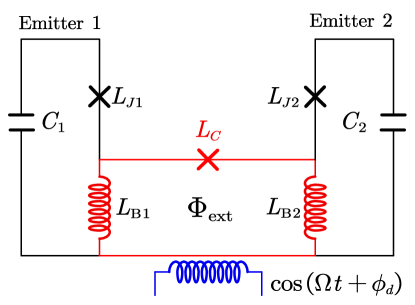
Figure S6: Schematic realization of parametric driving for two emitters. We
take circuit QED as an example, with two transmons in the form of
Josephson junctions (with effective inductances ) shunted by
their capacitances . The parametric coupling loop is composed of
two shared inductances and a coupling Josephson inductance
. To induce a time-dependent interaction, an external flux
is applied through the loop.
Based on the above cascaded quantum systems mediated by “correlated flying
qubits”, we show how to generate steady four-partite entangled states
between two remote nodes by applying additional parametric coherent drives to
the two GEPs. As depicted in Fig. S6, we take circuit QED
as an example.
Giant emitters 1 and 2 are coupled together via a Josephson loop, which is
composed of two shared branches with inductances and a Josephson
junction with an inductance . To realize a parametric drive on the two
emitters, we assume that a time-dependent flux through the loop is applied.
As discussed in Refs. [17, 18], the Hamiltonian of
the whole system is
(S76)
where the effective coupling between two emitters is controlled via the
external flux produced by the current in the coil. For simplicity, we assume
that the circuit parameters of the two emitters are identical, i.e.,
, , and . In the
limit , the relation between the coupling strength and the
external flux is [17]
(S77)
We assume that is composed of a dc and an ac part, i.e.,
. In the
limit , is approximately given by
(S78)
Given that , only the counter-rotating
terms in Eq. (S76) are resonant and should be kept. The
Jaynes–Cummings terms are rapidly
oscillating and can be neglected. In the rotating frame of emitter
frequencies, is reduced to a parametric-driving form, i.e.,
(S79)
where we set . When the parametric drives are applied to
both GEP A and B, the effective Hamiltonian in Eq. (S75) becomes
(S80)
We assume that the chiral factor is and that the two GEPs
exclusively emit correlated photons into the right direction. Similar to the
linear chiral quantum setups, the interplay between driving and chiral
dissipation leads to a dark state for the two GEPs [5]:
(S81)
By solving the above equation, we find that the two GEPs will be trapped in a
four-body entangled steady state
(S82)
Moreover, in the limit , the dark state is
approximately a four-body maximally entangled state
(S83)
By defining the fidelity , we plot the
time evolutions of the four emitters governed by in
Fig. S5(c), which shows that the two GEPs will be deterministically
trapped in the state in the steady state at long times. By
setting , we plot the fidelity and chiral factor as
functions of in Fig. S5(d). In the regions of right
emission with , the fidelity can reach . When
is biased away from the chiral regime, the whole setup becomes bidirectional,
and the fidelity for entangled states decreases accordingly, as shown in
Fig. S5(d).
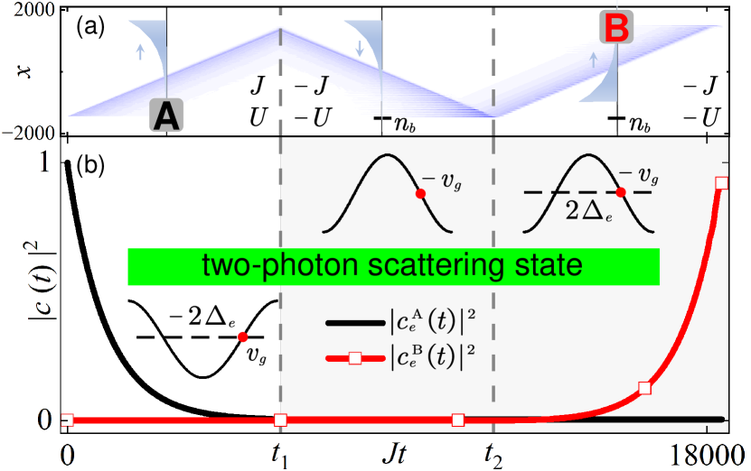
S4.2 Time-reversal operation for correlated-photon pulses
Figure S7: (a) The evolution of field distribution and
(b) populations for GEP A/B during the time-reversal operations for
the pulse of correlated photon pairs. At time , the signs of
and are reversed, and the dispersion relation is flipped by
keeping the momentum information, as depicted in the inset of (b). At
, the left-propagating field begins to be reflected by the break
point , and the pulse shape is time-reversed, which can be
absorbed by GEP B with a high efficiency. Here we set
, and the other parameters are the
same as in Fig. 2 in the main text.
We first prove that by changing the signs of and , the wave packet of
correlated photon pairs still retains the same shape, but with an opposite
propagation direction.
When , we set and . The
eigen-wavefunction for the nonlinear waveguide is , where satisfies Eq. (S6). The
corresponding eigenenergy is [see
Eq. (S15)]. We set the frequency of the GEP A to the
optimal point with [see Fig. 1(d) in
the main text]. Therefore, the GEP A spontaneously emits a photon pair in the
right direction. The wave packet, whose momentum is centered around ,
propagates along the waveguide with a positive group velocity . Its wave function is
(S84)
where is the amplitude for mode .
When , we reverse the signs of both the hopping rates and the
nonlinearity, i.e., and . It is easy to verify that
is still the eigen-wavefunction for the
waveguide because satisfies Eq. (S6), but the
eigenfrequency is reversed as [see
Eq. (S15)]. Therefore, the eigen-wavefunctions of the
nonlinear waveguide remain unchanged (i.e., preserving wave-vector
information), but the dispersion relation is reversed. When , the
wave packet is written as
(S85)
The group velocity is . Eventually, the wave packet maintains
its form while propagating in the opposite direction. When the pulse is
reflected by the boundary, its shape will be reversed compared to the
original wave packet emitted from GEP A.
Therefore, by reversing the signs of and , the proposed setup can be
engineered as a nonlinear phase-conjugate mirror for
doublons [19, 20], which can be employed for
high-fidelity entangled-state transfer processes. The detailed process,
illustrated in Fig. S7, for perfect absorption of the doublon wave
packet by controlling the system’s parameters is as follows:
i) . The GEP A (with total frequency ) emits a correlated photon pair, whose momentum is centred at .
The emitted pulse propagates chirally to the right in the waveguide with a
positive group velocity ; the wavefront is assumed to not yet reach GEP
B at .
ii) . We reverse the signs of and , and cut
off the hopping between sites and ( is on the left-hand
side of the pulse tail), as shown in the inset of Fig. S4(b). The
eigenwavefunctions of the nonlinear waveguide remain unchanged (i.e.,
preserve wave-vector information), but the dispersion relation is reversed as
. The group velocity is reversed as , and the
emitted field begins propagating to the left.
iii) At , the pulse begins to touch the breakpoint and is
reflected as a right-propagating photon pair. Compared with the original
pulse during , the shape of the wave packet is time-reversed.
In this scenario, the absorption by GEP B can be viewed as time-reversal
process of spontaneous emission, where the efficiency can approach 1.
In Fig. S7(a), we numerically simulate two-excitation transfer
between two GEPs; the evolution of the corresponding two-photon field is
plotted in Fig. S7(b). We find that the field shape of the
correlated photon pair is successfully reversed when and the
absorption efficiency is at . The infidelity is
mainly caused by intermediate single-photon states. We infer that, for a more
general case where GEP A initially is in the entangled state , this entangled state can be
deterministically transferred to GEP B with a high fidelity by following the
proposed protocol.
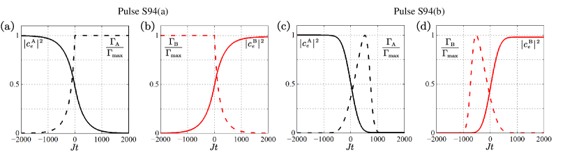
S4.3 State transfer via modulating the coupling strength
By modulating the decay rate with time, the shape of the directional wave
packet can be tailored freely. Under this mechanism, a perfect single-qubit
state transfer process via a photonic wave packet with time-reversal
symmetry, has been extensively explored in linear chiral
setups [21, 5, 22, 23]. In this
proposed nonlinear cascaded system, more quantum information can be encoded
into “correlated flying qubits”, and we show that a high-fidelity
entangled-state transfer between GEP A and B can be realized.
At time , the state of the cascaded system can be expanded as
(S86)
where () represents the two emitters of pair A (B)
both being excited, and denotes the waveguide in its
vacuum state. The dynamical phase factors are [24]
(S87)
where is the renormalized frequency of GEP A (B).
Note that the Stark shift of each emitter due to the single-photon scattering
state should be considered during state-transfer processes; it is given by
(S88)
(S89)
with the effective coupling strength. Note further
that when is modulated in time, the Stark shift for each
GEP will also be time-dependent.
Figure S8: Two-excitation transfer process between two GEPs. The solid
curves are the excitation probabilities of GEPs A and B. The dashed
curves correspond to the modulating pulses, which are given by
Eq. (S94c) for (a, b) and Eq. (S94d) for (c, d). The parameters
are the same as in Fig. 2 in the main text.
To realize a high-fidelity entangled-state transfer, we require that the
whole system satisfies the dark-state condition
(S90)
which restricts and [5]. Then, the evolution equations are
and
(S91)
(S92)
Additionally, the initial and final state should also satisfy the boundary
conditions
(S93)
where and are the initial and final times, respectively. For
convenience, we assume . As discussed in
Ref. [5], the following two types of control sequences can
meet all above conditions:
(S94c)
(S94d)
where , and is given by
Eq. (S48). Because , the modulating
pulse can be mapped as time-dependent coupling strengths
according to Eq. (S89) and Eq. (S94). In
Fig. S8, by fixing , we numerically plot the
two-excitation energy transfer from GEP A to B under the control of the two
pulse sequences in a finite waveguide with a length . Note that the
Stark shifts in Eq. (S89) are compensated by modulating the
frequencies of two GEPs oppositely, i.e., . We find that
the transfer efficiency can reach , which enables a high-fidelity entangled-state transfer
between two GEPs.
References
Piil and Mølmer [2007]R. Piil and K. Mølmer, “Tunneling
couplings in discrete lattices, single-particle band
structure, and
eigenstates of interacting atom pairs,” Phys.
Rev. A 76, 023607
(2007).
Wang et al. [2020]Z. Wang, T. Jaako,
P. Kirton, and P. Rabl, “Supercorrelated Radiance in Nonlinear
Photonic
Waveguides,” Phys. Rev. Lett. 124, 213601 (2020).
Stannigel et al. [2010]K. Stannigel, P. Rabl,
A. S. Sørensen,
P. Zoller, and M. D. Lukin, “Optomechanical Transducers for Long-Distance
Quantum Communication,” Phys. Rev. Lett. 105, 220501 (2010).
Stannigel et al. [2011]K. Stannigel, P. Rabl,
A. S. Sørensen,
M. D. Lukin, and P. Zoller, “Optomechanical transducers for
quantum-information processing,” Phys.
Rev. A 84, 042341
(2011).
Stannigel et al. [2012]K. Stannigel, P. Rabl, and P. Zoller, “Driven-dissipative
preparation of entangled states in cascaded quantum-optical
networks,” New J. Phys. 14, 063014 (2012).
Gu et al. [2017]X. Gu, A. F. Kockum,
A. Miranowicz,
Y.-X. Liu, and F. Nori, “Microwave photonics with superconducting
quantum
circuits,” Phys. Rep. 718-719, 1 (2017).
Krantz et al. [2019]P. Krantz, M. Kjaergaard,
F. Yan, T. P. Orlando, S. Gustavsson, and W. D. Oliver, “A quantum engineer’s guide to
superconducting
qubits,” Appl. Phys. Rev. 6, 021318 (2019).
Blais et al. [2021]A. Blais, A. L. Grimsmo,
S. M. Girvin, and A. Wallraff, “Circuit quantum electrodynamics,” Rev. Mod. Phys. 93, 025005 (2021).
Kannan et al. [2020]B. Kannan, M. J. Ruckriegel, D. L. Campbell, A. Frisk Kockum, J. Braumüller, D. K. Kim, M. Kjaergaard,
P. Krantz, A. Melville, B. M. Niedzielski, A. Vepsäläinen, R. Winik, J. L. Yoder, F. Nori, T. P. Orlando, S. Gustavsson, and W. D. Oliver, “Waveguide
quantum electrodynamics with superconducting artificial giant
atoms,” Nature 583, 775 (2020).
Vadiraj et al. [2021]A. M. Vadiraj, A. Ask,
T. G. McConkey,
I. Nsanzineza, C. W. S. Chang, A. F. Kockum, and C. M. Wilson, “Engineering the level structure of a giant
artificial atom in waveguide quantum electrodynamics,” Phys. Rev. A 103, 023710 (2021).
Joshi et al. [2023]C. Joshi, F. Yang, and M. Mirhosseini, “Resonance fluorescence
of a
chiral artificial atom,” Phys. Rev. X 13, 021039 (2023).
Koch et al. [2007]J. Koch, T. M. Yu,
J. Gambetta,
A. A. Houck, D. I. Schuster, J. Majer, A. Blais, M. H. Devoret, S. M. Girvin, and R. J. Schoelkopf, “Charge-insensitive qubit design derived from the Cooper pair
box,” Phys. Rev. A 76, 042319 (2007).
Ye et al. [2019]Y.-S. Ye et al., “Propagation and Localization of Collective Excitations on a
24-Qubit
Superconducting Processor,” Phys. Rev. Lett. 123, 050502 (2019).
Carusotto et al. [2020]I. Carusotto, A. A. Houck, A. J. Kollar,
P. Roushan,
D. I. Schuster, and J. Simon, “Photonic materials in circuit quantum
electrodynamics,” Nat. Phys. 16, 268 (2020).
Mansikkamäki et al. [2022]O. Mansikkamäki, S. Laine, A. Piltonen, and M. Silveri, “Beyond Hard-Core Bosons
in
Transmon Arrays,” PRX Quantum 3, 040314 (2022).
Xiang et al. [2023]Z.-C. Xiang, K. Huang,
Y.-R. Zhang,
T. Liu, Y.-H. Shi, C.-L. Deng, T. Liu, H. Li, G.-H. Liang,
Z.-Y. Mei,
H. Yu, G. Xue, Y. Tian, X. Song, Z.-B. Liu,
K. Xu, D. Zheng, F. Nori, and H. Fan, “Simulating Chern insulators on a superconducting quantum
processor,” Nat. Commun. 14, 5433 (2023).
Geller et al. [2015]M. R. Geller, E. Donate,
Y. Chen, M. T. Fang, N. Leung, C. Neill, P. Roushan, and J. M. Martinis, “Tunable coupler for superconducting Xmon qubits:
Perturbative
nonlinear model,” Phys. Rev. A 92, 012320 (2015).
Wulschner et al. [2016]F. Wulschner, J. Goetz,
F. R. Koessel,
E. Hoffmann, A. Baust, P. Eder, M. Fischer, M. Haeberlein,
M. J. Schwarz,
M. Pernpeintner, E. Xie, L. Zhong, C. W. Zollitsch, B. Peropadre, J.-J. Garcia-Ripoll, E. Solano, K. G. Fedorov,
E. P. Menzel,
F. Deppe, A. Marx, and R. Gross, “Tunable coupling of transmission-line microwave
resonators mediated by an rf SQUID,” EPJ Quantum Technol. 3, 10 (2016).
Yanik and Fan [2004]M. F. Yanik and S. Fan, “Time reversal of light
with
linear optics and modulators,” Phys. Rev. Lett. 93, 173903 (2004).
Wang et al. [2012]C. Wang, R. Martini, and C. P. Search, “Time-reversing light
pulses
by adiabatic coupling modulation in coupled-resonator optical
waveguides,” Phys. Rev. A 86, 063832 (2012).
Cirac et al. [1997]J. I. Cirac, P. Zoller,
H. J. Kimble, and H. Mabuchi, “Quantum State Transfer and
Entanglement
Distribution among Distant Nodes in a Quantum
Network,” Phys. Rev. Lett. 78, 3221 (1997).
Vermersch et al. [2017]B. Vermersch, P.-O. Guimond, H. Pichler, and P. Zoller, “Quantum State Transfer
via
Noisy Photonic and Phononic Waveguides,” Phys. Rev. Lett. 118, 133601 (2017).
Xiang et al. [2017]Z.-L. Xiang, M. Zhang,
L. Jiang, and P. Rabl, “Intracity Quantum Communication via Thermal
Microwave Networks,” Phys. Rev. X 7, 011035 (2017).