Mapping the anisotropic Galactic stellar halo with Blue Horizontal Branch stars

We use Legacy Survey photometric data to probe the stellar halo in multiple directions of the sky using a probabilistic methodology to identify Blue Horizontal Branch (BHB) stars. The measured average radial density profile follows a double power law in the range $5<r_{gc}/{\rm kpc}<120$, with a density break at $r_{gc}\approx 20$ kpc. This description, however, falls short, depending on the chosen line-of-sight, with some regions showing no signature of a break in the profile and a wide range of density slopes, e.g. outer slope $-5.5\lesssim\alpha_{out}\lesssim-4$, pointing towards a highly anisotropic stellar halo. This explains in part the wide range of density profiles reported in the literature owing to different tracers and sky coverage. Using our detailed 3-D stellar halo density map, we quantify the shape of the Pisces overdensity associated with the transient wake response of the Galaxy’s (dark) halo to the Large Magellanic Cloud (LMC). Measured in the LMC’s coordinate system, Pisces stands above the background, is 60 degrees long and 25 degrees wide and aligned with the LMC’s orbit. This would correspond to a wake width of $\sim 32$ kpc at $\sim 70$ kpc. We do not find a statistically significant signature of the collective response in density as previously reported in the literature measured with K giant stars, despite our larger numbers. We release the catalogue constructed in this study with 95,446 possible BHB stars and their BHB probability.

1 Introduction

The Milky Way’s (MW) stellar halo provides valuable information about the Galaxy’s history since it contains most of the metal-poor, ${\rm[Fe/H]}\,<\,-1$, and oldest stars, age $>10$ Gyr (e.g. Beers & Christlieb 2005; Frebel & Norris 2015; Das et al. 2020). Although it is the most extended baryonic component of the Galaxy, reaching out to $\approx$ 200 kpc, its stellar content only contributes around 2% to the total stellar mass of the Galaxy (e.g., Deason et al. 2019). Moreover, the stellar halo is not smooth, but is comprised of substructures from globular clusters (e.g. Myeong et al. 2018; Massari et al. 2019; Forbes 2020; Limberg et al. 2022), to debris from past accretion events (e.g. Helmi et al. 1999; Koppelman et al. 2019; Naidu et al. 2020; Yuan et al. 2020; Limberg et al. 2021; Malhan et al. 2022), and satellite dwarf galaxies (e.g. McConnachie 2012). Throughout the manuscript, we will refer to the Galactic stellar halo as the “halo” unless otherwise explicitly stated when referring to the dark matter halo of the MW.

Determining the structure of the MW halo involves counting stars across the sky. With the current photometric surveys, this task is limited by dust extinction, the survey’s magnitude limit and its footprint, which are encoded into the survey selection function. Knowing the survey selection function is crucial for a rigorous approach to measuring the radial density profile of the halo in order to interpret observations with theoretical models. For instance, a non-smooth halo would imply a recent merging activity whereas a smooth one would reveal a more quiescent formation history (Johnston et al. 2008; Deason et al. 2013). We expect both, with varying degrees of contributions, in the hierarchical formation scenario (e.g. Searle & Zinn 1978; White & Frenk 1991; Springel et al. 2006).

Despite the difficulties in obtaining a sample of stars that homogeneously covers the Galaxy, numerous studies mapped the halo density profile albeit with a not-well-established consensus on the shape of the profile. The radial density profile has typically been described by a single-, double-power law, or Einasto profile (e.g. Deason et al. 2011; Xue et al. 2015; Hernitschek et al. 2018; Wu et al. 2022b) with the choice adopted partially due to the sample and survey limitations. A halo described by a double power law also defines the radius at which the inner and outer slopes change, known as the break radius, $r_{br}$.

Deason et al. (2013) showed that a broken radial density profile is a signature of apocenter pile-ups of accreted dwarf galaxies. They studied the radial density profiles of idealized simulations with accreted satellites from Bullock & Johnston (2005) and argued that the presence of a break radius results from a massive merger event, i.e. a merger that contributes the most to the total stellar halo mass. They concluded that the presence of a break radius in the MW stellar halo density profile is, therefore, a signature of a massive merger event (see e.g. Brook et al. 2003; Gilmore et al. 2002; Meza et al. 2005 for other signatures of the same merger). Recently, the accreted dwarf that dominates the MW stellar halo, and likely causes the observed broken profile, was identified as the Gaia-Sausage/Enceladus (GSE; Belokurov et al. 2018; Helmi et al. 2018; Haywood et al. 2018) and is estimated to constitute up to 3/4 of the inner ($r_{gc}<30$ kpc) stellar halo (e.g. Wu et al. 2022a, but see also Lane et al. 2023). Interestingly, Han et al. (2022) and Yang et al. (2022), using different methodologies, found evidence for a doubly broken halo density profile, and associated the two break radii with the pericenters of the GSE orbit (Naidu et al. 2021).

Since then, the GSE debris properties have been extensively studied taking advantage of the Gaia data combined with large spectroscopic surveys. Its stellar mass, peak [Fe/H] and time of merger range from $0.15-1\times 10^{9}$ $\,\mathrm{M_{\odot}}$  (e.g. Feuillet et al. 2020; Naidu et al. 2020; Limberg et al. 2022; Lane et al. 2023), $-1.45<{\rm[Fe/H]}<-1.17$ (e.g. Amarante et al. 2020; Bird et al. 2021; Liu et al. 2022), 8-11 Gyr (e.g. Gallart et al. 2019; Montalbán et al. 2021; Xiang & Rix 2022), respectively. The differences arise from distinct selection criteria and samples used (see e.g. Carrillo et al. 2024 for a discussion). Despite the GSE merger event being estimated to have happened 10 Gyr ago, part of its debris is argued as being not completely phase-mixed. For instance, the Hercules-Aquila Cloud South and North (HAC-S, HAC-N, Belokurov et al. 2007a; Watkins et al. 2009; Simion et al. 2014) and Virgo Overdensity (VOD, Vivas et al. 2001; Newberg et al. 2002; Jurić et al. 2008) – overdensities observed in the stellar halo – are chemodynamically consistent with GSE stars (Simion et al. 2019; Perottoni et al. 2022). These substructures, except for HAC-N, have been argued to be a consequence of the GSE merger as seen in pure N-body models (Naidu et al. 2021). On the other hand, Donlon et al. (2020, 2023) argue that the presence of these substructures indicates a more recent time for the merger, circa $\sim$2–3 Gyr ago.

While the GSE debris is likely to dominate the stellar halo within the break radius, at larger distances, a more heterogeneous stellar halo, built from the debris of several other minor accretions, is found. The outer halo also comprises a myriad of known dwarf-satellite galaxies bound or in the process of being engulfed by the MW (e.g. Belokurov et al. 2007b; Koposov et al. 2015; Pace et al. 2022; Cerny et al. 2023). For instance, ongoing accretion events are observed for the Saggitarius dwarf (Sgr, e.g. Ibata et al. 1994; Johnston et al. 1995), and Small and Large Magellanic Clouds (SMC, LMC, e.g. Besla et al. 2007). Due to their relatively massive nature, pure N-body simulations of these two systems put into question the “Galaxy in equilibrium” approximation. The stellar content and the dark matter halo of the MW are strongly perturbed due to the interaction with Sgr (e.g Purcell et al. 2011; Gómez et al. 2013; Laporte et al. 2018b, 2019; Carr et al. 2022; Borbolato et al. 2023), and the LMC (e.g. Weinberg & Blitz 2006; Laporte et al. 2018a; Petersen & Peñarrubia 2020; Garavito-Camargo et al. 2019; Vasiliev 2023).

The LMC should induce a gravitational wake in the MW dark matter distribution and cause the sloshing of the stellar halo. In a classical Chandrasekhar (1943) sense from stars, and dark matter, being deflected behind the LMC’s orbit. Thus, the LMC’s orbit wake should create an overdensity in the stellar halo, known as the “transient wake” (Weinberg 1998; Laporte et al. 2018a; Garavito-Camargo et al. 2019; Petersen & Peñarrubia 2020; Erkal et al. 2021; Garavito-Camargo et al. 2021). Besides that, the movement of the MW-LMC system barycenter (Gómez et al. 2015) can also create a signature in the dark matter halo and consequently imprinted on the stellar component, namely the “collective response” (Weinberg 1989, 1998; Garavito-Camargo et al. 2019; Cunningham et al. 2020; Petersen & Peñarrubia 2021). Numerical work also predicts an overdensity of LMC-stripped stars at the track of the LMC orbit (Petersen et al. 2022).

Recently the Pisces overdensity (Sesar et al. 2007; Watkins et al. 2009; Kollmeier et al. 2009; Nie et al. 2015) has been interpreted as a signature of the local wake on the stellar halo (Belokurov et al. 2019). This has been corroborated further with K-giants by Conroy et al. (2021) which also suggested a detection of the collective response in star counts. To further complicate matters, retrograde debris has also been associated with GSE debris in the region close to Pisces (Chandra et al. 2023b).

Given these various contributions to the stellar halo, i.e. different accretion events and dynamical processes, a single-density profile would fall short of describing its complex structure. Ideally, by probing the whole sky with a homogeneous sample, one can measure any spatial dependence on the density profile. In fact, Hernitschek et al. (2018) has done it using RR-Lyrae from the Pan-STARRS1 survey (Sesar et al. 2017b) and fitted the stellar halo density profile for several bins in Galactic longitude, $l$ and Galactic latitude, $b$, with $30^{\circ}$ and $60^{\circ}$ width, respectively. After removing known overdensities, they concluded that the stellar halo is well fit either by a single power law or an Einasto profile in all directions, which at face value would be considered at odds with a broken profile and with an out-of-equilibrium MW stellar halo.

Probing the stellar halo at large distances depends on measuring accurate stellar distances. Currently, this is mainly done with “standard candles”. These are stars with relatively well-defined distance-module relations, such as red giant branch (RGB), RR Lyrae, and blue horizontal branch (BHB) stars. In this work, we will rely on BHB stars as they are in general associated with the MW stellar halo due to their old age (Dotter et al. 2010) and low metallicity (Santucci et al. 2015).

BHB stars have a relatively well-defined absolute magnitude range (e.g. Sirko et al. 2004) and they can be identified photometrically in the colour range, $-0.3<g-r<0$ (e.g. Yanny et al. 2000; Deason et al. 2011). Although spectroscopy is necessary to confirm BHB stars (e.g. Vickers et al. 2012; Barbosa et al. 2022), an appropriate colour selection can identify BHB stars with high confidence (e.g. Belokurov & Koposov 2016; Li et al. 2019; Starkenburg et al. 2019).

In this work, we use Legacy Survey data release 9 to probe the stellar halo density profile with BHB candidates. However, our measurement does not rely on identifying individual BHB stars. Similarly to Deason et al. (2011), we developed a methodology which takes into account the survey footprint, and for a given spatial selection, we measure the BHB fraction from the colour-colour distribution in a probabilistic fashion. This allows us to robustly estimate the halo density profile with its associated errors.

This paper is organised as follows: in Section 2 we present the Legacy Survey data selection and cleaning. In Section 3 we describe the methodology to calculate the BHB star fraction at a given spatial and magnitude selection, and how we model the radial density profile. We proceed by showing the density profiles for the MW, known overdensities regions, and several patches in the sky with high angular resolution, compared to previous studies, in Section 4. We discuss the implications of our findings for the structure of the MW stellar inner and outer halo in Section 5. Finally, in Section 6 we summarize our work and discuss future prospects.

2 Data

In this section, we briefly describe the Legacy Survey, the colour selection to discriminate BHB star candidates and possible sources of contamination.

2.1 Legacy Survey data selection

We use data from the Legacy Survey data release 9 (LSDR9 Dey et al. 2019). LSDR9 cover a total area of 14,000 deg², in the region $-18^{\circ}<\delta<+84^{\circ}$ and galactic latitude $|b|>18^{\circ}$. The data contain measurements of the $g$, $r$, $z$ photometric bands reaching a magnitude depth of approximately 24, 23.5 and 22.5 respectively. Its photometry coverage makes it an excellent database for photometrically identifying BHB star candidates.

We initially select objects within the extinction corrected colour intervals $-0.4<(g-r)<0.2$ and $-0.7<r-z<0.1$, and within the apparent magnitude range $12<g<24$. The first step of the data processing consisted of applying the LSDR9 bitmasks 12 and 13 which remove pixels touching a large galaxy and globular cluster, respectively. We also applied the $g,r,z$ bands offset correction given by Zhou et al. (2023). They showed the presence of an offset between LSDR9 with Gaia synthetic photometry which is also strongly correlated with sky position. We stress the importance of this correction, as without it, any colour-based study can be severely biased.

2.2 Colour-colour space

Figure 1 shows the $(g-r)\times(r-z)$ plane of our initial sample. BHB stars are well known to lie within $-0.3<(g-r)<0$ (e.g. Deason et al. 2011; Belokurov & Koposov 2016) and this is our starting point to define the BHB fraction in a probabilistic fashion. Li et al. (2019) defined the boundaries for BHB stars using $(g-r)$ and $(r-z)$ colours, and here we re-write their relation defining the $grz$ colour:

$$\begin{split}grz=&1.07163(g-r)^{5}-1.42272(g-r)^{4}+\\ &0.69476(g-r)^{3}-0.12911(g-r)^{2}+\\ &0.66993(g-r)-0.11368-(r-z),\end{split}$$ (1)

where BHB stars are scattered around $grz\approx 0$.

As seen in Figure 1, the region associated with BHB stars, within the dashed blue lines, is within the limits of previous studies. This is reassuring as, although we use the same photometric band, the calibration of LSDR9 could be significantly different to offset the BHB relation. Compared to previous studies, we only slightly modified the range on $(g-r)$ colour. Thus, throughout the paper, we only consider stars satisfying the following colour criteria:

$$\begin{split}&-0.14<grz<0.07\\ &-0.30<(g-r)<-0.05\end{split}$$ (2)

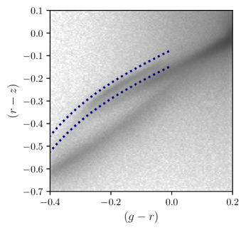
Figure 1: The $(g-r)\times(r-z)$ diagram for the first selected LSDR9 objects. The blue dotted lines are the boundaries for selecting BHB star candidates following Li et al. (2019).

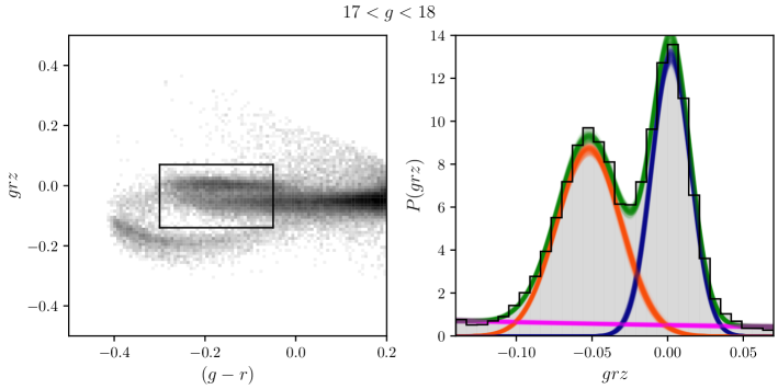
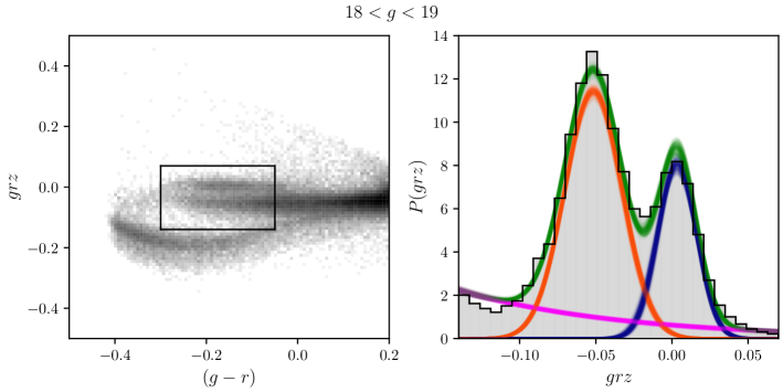
Figure 2: The left panels show $grz$ colour, see Equation 1, as a function $(g-r)$ at different $g$ ranges. The right panels show the $P(grz)$, in grey, of the stars within the selection box on the left panel. The corresponding fit to the data following Equation 3 as well as the BHB, BS and background component are represented in green, blue, orange and magenta, respectively. These two examples are part of the exercise illustrated in Figure 3 which assumes flat priors for the free parameters. Throughout this paper, we do use Gaussian priors for the BHB stellar component when calculating the BHB stellar densities, see Section 3.1 for details.

2.3 Possible sources of contamination

The colour-colour selection defined in Section 2.2 can be contaminated by blue stragglers (BS), quasars, and white dwarfs (see e.g Vickers et al. 2012). In the next section, we will explicitly take into account the BS contamination, and here we apply some criteria to minimize the number of quasars and white dwarfs contaminants.

At faint magnitudes and towards bluer colours, there is an increasing number of quasars among all the observed objects. Moreover, quasars have a large scatter over the colour space due to their different spectral energy distributions and redshifts (see e.g. Ross et al. 2012). To remove potential quasar objects, we use the fluxes on the LSDR9 $r-$band and the Wide-field Infrared Survey Explorer (WISE, Wright et al. 2010) photometric band $W1$, as the quasar’s dust emission makes them extremely bright in the $r-$band. We include the criterion $-0.09<{\rm F}_{W1}/{\rm F}_{r}<0.45$ to select objects of interest, where $F_{W1}$ and $F{r}$ are the observed fluxes in $W1$ and $r$, respectively. This selection is motivated by the fact that typical quasar objects have $F_{W1}/F_{r}\gtrsim 0.45$.

To estimate the amount of contamination from white dwarfs, we used the Gaia EDR3 white dwarf catalogue (Gentile Fusillo et al. 2021) and verified that they have negligible contamination in the BHB region of this work. For instance, white dwarfs start to populate the selection box for $g>17$ but mostly in the redder part of the $grz$ colour. See Appendix A for details.

We also removed stars that lie within 5 times the effective radius of known dwarf galaxies from McConnachie (2012) catalogue, except for the Large and Small Magellanic Clouds (LMC, SMC) which we removed stars within an angular separation of 12.5 degrees and 6.5 degrees from their centres, respectively. Finally, we also mask the region with $|\tilde{B}_{sgr}|<10.5^{\circ}$, where $\tilde{B}_{sgr}$ is the Sgr stream coordinate system as defined in Belokurov et al. (2014).

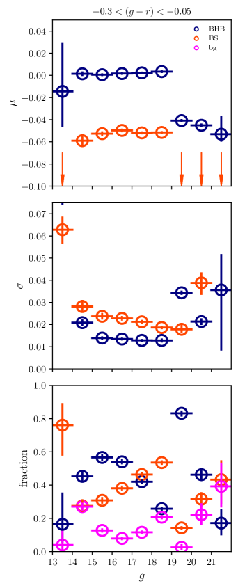
Figure 3: The variation of the free parameters while fitting Equation 3 as a function of $g$ assuming flat priors. While the horizontal lines correspond to the $g$ interval on which the fit was performed, the vertical lines correspond to the 16th-84th interval of the posterior distribution. The BHB stellar parameters are relatively constant within $15<g<19$ which motivated the use of Gaussian priors throughout this work, see Section 3.1 for discussion.

3 Methodology

In the previous section, we defined the colour-colour selection, Equation 2, of the main sample which contains most of the BHB stars, and removed contamination from other sources, namely quasars and white dwarfs. The top left panel in Figure 4 shows the Mollweide projection in Galactic coordinates, ($\ell,b$) of the stars satisfying these criteria. We now proceed with the methodology to obtain the fraction of BHB stars.

3.1 BHB stars fraction

For any given selection within our sample, the BHB stars’ contribution to the $grz$ distribution can be modelled as a Gaussian component with mean $\mu=0$ and dispersion, $\sigma$, due to the errors and scatter of the relation given by Equation 1. We illustrate this in Figure 2 where we show the $grz$ histogram for stars within two different $g$ intervals. In the first example, in the magnitude range $17<g<18$, the $grz$ colour distribution has a double peak shape, each associated with the BHB and BS components. Thus, we model the $grz$ probability density distribution, $P(grz)$, as a two-component Gaussian mixture with an additional exponential component representing other contaminant sources missed in the data cleaning of the previous section, i.e.:

$$P(grz)=w_{1}P(grz|BHB)+w_{2}P(grz|BS)+w_{3}P(grz|OTH)$$

$$=w_{1}G(grz,\mu_{1},\sigma_{1})+w_{2}G(grz,\mu_{2},\sigma_{2})+w_{3}\exp(\beta grz)$$ (3)

where $G(x,\mu_{i},\sigma_{i})$ is the probability density function (PDF) of the Normal distribution for the BHB and BS components with mean $\mu_{i}$ and standard deviation $\sigma_{i}$. The background exponential is characterised by the parameter $\beta$. The contribution fraction of each component is given by $w_{i}$, and their sum equals 1. Therefore, there are a total of eight free parameters.

Selecting BHB star candidates using a probabilistic model based on the star’s photometry (e.g. Deason et al. 2014; Thomas et al. 2018; Starkenburg et al. 2019; Yu et al. 2024) or based on spectroscopic parameters (Sirko et al. 2004; Xue et al. 2011; Santucci et al. 2015; Barbosa et al. 2022) and model their spatial distribution has been extensively explored. However, these approaches fail to select BHB stars at the faint end of the magnitude range, where the photometric or spectroscopic uncertainties are large and the overlap between BS and BHB is significant. The methodology presented in this work lies in estimating the number (or fraction) of BHB stars at any given selection within our sample, instead of selecting individual objects based on their probabilities (see, e.g. Deason et al. 2011; Fukushima et al. 2019).

We estimate the number of BHB stars by fitting the distribution given by Equation 3 and sample the model with the Affine Invariant Markov Chain Monte Carlo (MCMC) sampler, implemented in the emcee package (Foreman-Mackey et al. 2013). This allows us to obtain an error estimation from the posterior distribution of the eight free parameters of Equation 3. For each $w_{bhb,i}$ posterior, we calculate the number of BHB stars, $N_{bhb,i}$, as:

$$N_{bhb,i}=w_{bhb,i}*N_{P,i},$$ (4)

where $N_{P}$ is a random number drawn from a Poisson distribution with observed objects $\lambda=N_{tot}$, $N_{tot}$ is the total number of objects within a given magnitude and/or spatial selection, and $i$ is the posterior index. From the posterior distribution, we use the 50th percentile as the value of $N_{bhb}$, and the difference between the 84th and 16th percentiles as its error. We now proceed with a few tests to verify any dependence on colours and $g$-band for the BHB Gaussian component, $(\mu_{bhb},\sigma_{bhb})$, which could affect the modelling in the next section.

3.1.1 BHB star fraction test

We select stars with $-0.30<(g-r)<-0.05$ and fit the $grz$ distribution using Equation 3, including the errors of $grz$, for several intervals in $g$-band. Here we use flat priors for all the parameters. The right column of Figure 2 shows two examples of the fitting. While for the intervals shown the BHB stellar component is centred around $grz\approx 0$, this is not the case for the fainter intervals, $g>19$, where the flat priors fail to provide a good fit for the data. In fact, for the interval $15<g<19$, $\mu_{bhb}$ and $\sigma_{bhb}$ are relatively constant and they only deviate for stars at the very bright and faint end. This is seen in Figure 3 which shows the results of the $\mu$ and $\sigma$ for the BHB and BS components as well as their fractions for several $g$-band intervals. At the faint magnitude range, the errors in the $grz$ colours are larger and thus strongly affect the BHB Gaussian distribution.

Santucci et al. (2015) showed that BHB stars identified spectroscopically have a shift in the $(g-r)$, being redder towards larger distances, due to an age difference of $\sim 2$ Gyr. Motivated by this, we repeated the previous exercise for two colour intervals, $-0.3<(g-r)<-0.175$ and $-0.175<(g-r)<-0.05$, and verified that, for $P(grz)$ given by Equation 3, $\mu_{bhb}$ and $\sigma_{bhb}$ are consistent between the two intervals.

Based on these results, for the analysis described in the next sections, we complement the log-likelihood from Equation 3 by Gaussian priors on $\mu_{bhb}$ centred on 0.0005 with a width of 0.0005, and on $\sigma_{bhb}$, centred on 0.014 with a width of 0.001. We assume flat priors for $\mu_{bs}$, $\sigma_{bs}$, $\beta$, and the fractions $w_{i}$. Finally, in the next section, we included the criteria:

$$14.5<r<21.5,$$ (5)

avoiding saturation problems of LSDR9 photometry and completeness in the bright and faint ends, respectively.

3.2 BHB stars density

We now proceed and describe how we calculate the radial density profile for any given volume within the LSDR9 footprint. We use the BHB absolute magnitude relation from Belokurov & Koposov (2016):

$$\begin{split}M_{g,bhb}=&0.398-0.392(g-r)_{0}+2.729(g-r)_{0}^{2}+\\ &29.1128(g-r)_{0}^{3}+113.569(g-r)_{0}^{4},\end{split}$$ (6)

convert to heliocentric distance using the distance-modulus equation, and calculate the Cartesian Galactocentric coordinates, $(x,y,z)$, assuming the Sun’s position $(X_{\odot},Y_{\odot},Z_{\odot})=(-8.2,0,0.027)$ kpc (McMillan 2017; Bennett & Bovy 2019).

The stellar halo of the MW is also known to be flattened (e.g. Iorio et al. 2018; Hernitschek et al. 2018; Wu et al. 2022b; Yang et al. 2022), therefore we calculate the density profiles as a function of the flattened radius:

$$r_{q}=\sqrt{x^{2}+y^{2}+\left(\frac{z}{q(r)}\right)^{2}},$$ (7)

with $q$ being the flattening parameter. Although it is consistently found that the inner halo is flattened while the outer halo is more spherical, there is no consensus on how flat the MW halo truly is and whether its flattening varies with Galactocentric radius or not. It is out of the scope of the current work to fit for the parameter $q$, thus we assume $q=0.77$ for $r<30$ kpc and $q=0.99$ otherwise. This is motivated by results found in Hernitschek et al. (2018) and is in good agreement with the range of values found in the literature. We also verified that the results discussed below hold for different values of $q$ that can be found in the literature.

A necessary ingredient for spatial density estimation is not only the estimate of the number of stars but also the volume covered by the survey. We can explicitly calculate the volume encompassed by a sample defined within a Galactocentric distance-module range, i.e.:

$$a<g_{0}-M_{g,bhb}<b,$$ (8)

where $g_{0}$ is the extinction corrected apparent magnitude in the $g-$band and $M_{g,bhb}$ is given by Equation 6. For the same volume, we can also estimate $N_{bhb}$ and its error as described in Section 3.1 thus providing us with the estimate of the BHB number density, $n_{bhb}$, and its error, $n_{bhb,er}$, within the volume constrained by Equation 8 and the LSDR9 footprint.

3.3 Radial density profiles

The methodology described in the previous sections allows us to construct the radial density profile for the full LSDR9 footprint as well as for any direction or patch in the sky. Throughout this work, we fit the number density profiles with a double power law model:

$$n(r_{q})=\begin{cases}n_{\odot}r_{q}^{\alpha_{in}},&\text{if }r_{q}<r_{br}\\ n_{\odot}r_{br}^{\alpha_{in}}(r_{q}-r_{br})^{\alpha_{out}},&\text{otherwise}\end{cases}$$ (9)

where $n_{\odot}$ is the local density normalization, $r_{br}$ is the break radius, and $\alpha_{in}$/$\alpha_{out}$ is the inner/outer slope.

In the next section, we construct the density profiles calculating the BHB density and its error estimated as in Section 3.1 at several bins in Galactocentric distance. Ideally, it is preferred to perform a fitting using all the available data points and not binned data, but our methodology relies on calculating the probabilistic fraction of BHB stars, and not identifying them individually. Therefore, we follow the approach of Anders et al. (2021) and estimate the free parameters of Equation 9 minimising the $\chi^{2}$ function using the binned profile and taking into account the error in $n_{bhb}$. We use flat priors for all the four free parameters: $n_{\odot}$, $r_{br}$, $\alpha_{in}$, and $\alpha_{out}$, and emcee to sample from the posterior distributions. We take the median values as the parameter values, and the errors are from the 16th and 84th percentiles.

4 Results

With the data selection and methodology described in Sections 2 and 3, respectively, we now explore the Galactocentric radial density profile of the MW, as observed with LSDR9, and of regions with known identified substructures in Section 4.1, proceed to a higher angular resolution radial profile in Section 4.2, and depict the anisotropy of the stellar halo in Section 4.3.

Name	(l,b) [deg]	$d_{\odot}$ [kpc]	$r_{br}$ [kpc]	$(\alpha_{in},$ $\alpha_{out})$
HAC-S	$30^{\circ}<l<60^{\circ}$, $-45^{\circ}<b<-20^{\circ}$	10-20	$24.8^{+0.8}_{-1.0}$	$(-3.0^{+0.1}_{-0.1},$$-5.3^{+0.2}_{-0.2})$
HAC-N	$30^{\circ}<l<60^{\circ}$, $20^{\circ}<b<45^{\circ}$	10-20	$22.3^{+1.3}_{-1.2}$	$(-2.8^{+0.2}_{-0.2},$$-5.7^{+0.3}_{-0.3})$
VOD	$270^{\circ}<l<330^{\circ}$, $-45^{\circ}<b<-20^{\circ}$	10-20	$22.4^{+3.6}_{-3.4}$	$(-2.8^{+0.4}_{-0.3},$$-4.2^{+0.2}_{-0.2})$
Pisces	$(74^{\circ},-47^{\circ})$	60-100	–	$(-3.8^{+0.7}_{-2.5},$$-3.8^{+0.2}_{-0.3})$

Table 1: The Galactic coordinates and heliocentric distance used in this work for Hecules-Aquila Cloud South/North (HAC-S/N, Belokurov et al. 2007a; Watkins et al. 2009; Sesar et al. 2010; Simion et al. 2014), Virgo Overdensity (VOD, Jurić et al. 2008; Bonaca et al. 2012), and Pisces (Nie et al. 2015; Belokurov et al. 2019). For the latter, we indicate the centre of a $20^{\circ}$ region satisfying the regions associated with Pisces as in Belokurov et al. (2019) and Conroy et al. (2021). We also show the slopes and break radius, $r_{br}$, of a two-power law fit of these regions obtained in this work.

4.1 The radial density profile of the MW and known overdensities

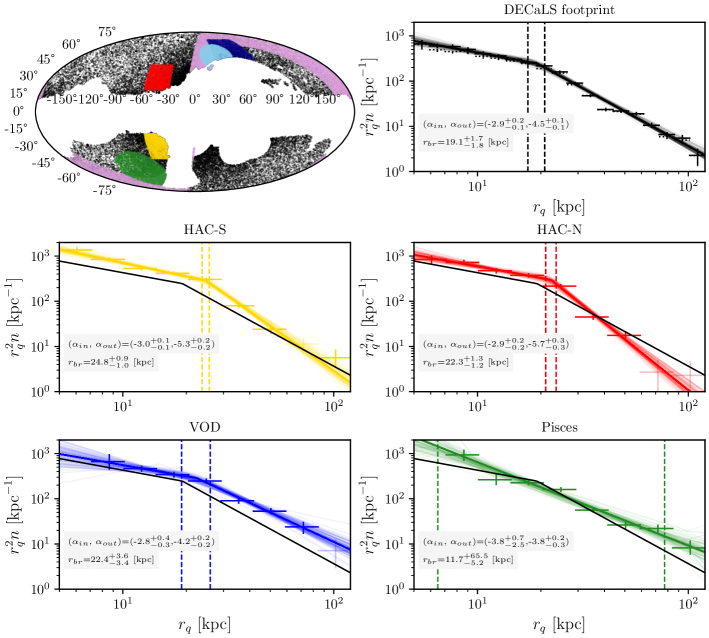
Figure 4: Top left panel: The Galactic Mollweide projection of LSDR9 stellar objects selected using Equation 2. The highlighted regions represent the location of known substructures: Sagittarius stream (pink), HAC-S (yellow), HAC-N (red), Pisces (green), VOD (blue) and OVO (cyan). Top right panel: The Galactocentric BHB stellar density profile of the whole LSDR9 footprint and without HAC-S, HAC-N and VOD regions as the solid and dotted markers, respectively. Bottom panels: The Galactocentric radial density profiles for the Galactic regions associated with HAC-N, HAC-S, VOD and Pisces. The crosses correspond to twenty and ten radial bins equally spaced in logarithm within $5<r_{q}/{\rm kpc}<120$ for LSDR9 footprint and overdensities, respectively. We also show the resulting fit for 100 samples drawn from the posterior distribution as the solid lines.

The top right panel in Figure 4 shows the Galactocentric radial density profile for the whole LSDR9 survey sky coverage. The BHB stars average profile has a clear break at $r_{q}=19.1^{+1.7}_{-1.8}$ kpc with inner and outer slope $(\alpha_{in},\alpha_{out})=(-2.85^{+0.17}_{-0.14},-4.55^{+0.11}_{-0.10})$. The location of the break and the inner and outer slopes are within the range of previously identified broken power law profiles in the MW halo, see for example table 6 in Medina et al. (2024) for a compilation of literature stellar halo density profiles. We defer the discussion and comparison with previous density profile estimations to Section 5.

The MW stellar halo harbours several substructures/overdensities that could potentially alter its density profile shape and some of them have been linked to previous merger events. We identify the regions associated with Hercules Aquila Cloud North & South (HAC-N & HAC-S), Virgo Overdensity (VO) and Pisces overdensity, whose coordinates are given in Table 1, in the top panel of Figure 4 as the coloured regions. We proceed and characterise the regions associated with the overdensities in the inner halo, $r_{q}<30$ kpc, HAC-N/S and VOD, and outer halo, Pisces. The second and third rows in Figure 4 show their radial density profile. The coloured markers correspond to the selected regions and the black solid line to the full LSDR9 profile, i.e. the average profile.

HAC-N, HAC-S and VOD have a broadly similar profile with a clear break radius, at the same position as the average profile, $r_{q}\approx 20$ kpc, and their slopes are within the errors as those estimated for the average sky. VOD shows an excess above the average density at all radii, while HAC-S and HAC-N only have excess within $r_{q}<20$ kpc, i.e. within the distance range previously reported in the literature. Moreover, HAC-N/S have a steeper outer slope compared to the average profile and VOD.

Noteworthy, this is the first time the radial density profile of these regions is shown for a large distance extension, $5<r_{q}/{\rm kpc}<120$, which allows showing clear evidence for the presence of a broken radial profile. HAC-S/N and VOD regions are known to be populated with stars with similar chemodynamical properties associated with the GSE merger (Simion et al. 2019; Perottoni et al. 2022). Nonetheless, in Section 4.2 we show that these overdensities profiles are consistent with the Galactocentric quadrants where they are located.

As HAC-N, HAC-S, and VOD have been associated with GSE, which likely dominates the stellar halo mass content, and they show a clear signature of a broken profile, one could argue that the global profile is broken due to the presence of these regions. We thus mask these three regions, as defined in Table 1, and recalculate the global density profile. However, after removing HAC-N, HAC-S and VOD, the shape of the halo is still well represented by a broken power law, dotted markers in Figure 4 top right panel, at odds with Hernitschek et al. (2017) whose methodology favours a single power law after removing these substructures. We stress, however, that we probe the halo from $5$ to $120$ kpc, while Hernitschek et al. (2017) only for $r_{q}>20$ kpc. Nonetheless, the outer slope of our profile is in agreement with the slope these authors found.

Among the regions with substructures, the Pisces region is the only one that shows no evidence of a break in its density profile. This is seen both in Figure 4 but also in measurements of the inner and outer slopes, which are consistent within uncertainties, as well as by the fact that the break radius is not well constrained. Pisces overdensity was identified at large radii, and here we detect excess in its profile at $r_{q}>50$ kpc. At its direction, there is also an overdensity at $r_{q}\approx 8$ kpc not previously reported. Furthermore, the density profile in its direction is less steep than the average outer stellar halo density profile.

The behaviour of the density profile in four different regions hints at an anisotropic density profile of the MW stellar halo which could be “direction-dependent” rather than being described by a single density profile stratified on simple surfaces like ellipsoids. Motivated by this, we proceed to study the radial density profile for several regions in the sky as seen in the Galactocentric angular coordinate system.

4.2 The radial density profile at distinct Galactocentric angular coordinates

In this subsection, we show the radial density profile in several Galactocentric directions. We convert from Galactocentric Cartesian $(x,y,z)$ to spherical coordinates and define the spherical angles $\Theta_{gc}$ and $\Phi_{gc}$ as the Galactocentric longitude and latitudes, respectively:

$$\Theta_{gc}=\arctan{\frac{z}{\sqrt{x^{2}+y^{2}}}}, \Phi_{gc}=\frac{y}{x}$$ (10)

Figure 5: The Galactocentric radial density profiles for the four quadrants of the Galactocentric projected sky. The crosses correspond to ten radial bins equally spaced in logarithm within $5<r_{q}/{\rm kpc}<120$. We also show the resulting fit for 100 samples drawn from the posterior distribution as the brown solid lines. The histogram corresponds to the posterior distribution of the break radius, $r_{br}$, and the dashed vertical lines are the corresponding 16th and 84th percentiles. The density profile of the full LSDR9 footprint, HAC-N, HAC-S, VOD and Pisces are shown as the black, red, yellow, blue, and green lines, respectively.

We first show the density profile for the four quadrants of the Galactocentric projected sky in Figure 5. We do not remove the substructures located within each quadrant. While the four quadrants have signatures of a break and similar outer slopes, within the errors, they differ in the steepness of the inner slopes, $\alpha_{in}$. For instance, the profile of the second ($\Phi_{gc}>0,\Theta_{gc}>0$) and fourth ($\Phi_{gc}>0,\Theta_{gc}>0$) quadrants are not as steep as the first ($\Phi_{gc}<0,\Theta_{gc}>0$) and third ($\Phi_{gc}<0,\Theta_{gc}<0$) ones.

There are also noticeable differences when comparing the profile of the regions associated with substructures to the Galactocentric quadrants in which they are located. HAC-N shows a distinct inner density profile, within the break radius, compared to the second quadrant, where it is located. This is shown in the left panel of Figure 5, where the brown markers represent the radial density for the quadrant and the red line is the best fit for HAC-N, as in the previous section. This quadrant’s profile closely follows the average profile (solid black line) in the inner parts, even without masking HAC-N when measuring it, in contrast to HAC-N. This reinforces the presence of HAC-N as a genuine overdensity, as this region neither follows the global profile nor that of the quadrant it is located.

The third quadrant, shown in the bottom left of Figure 5, includes two overdensities regions: HAC-S and Pisces, whose profiles are shown as the yellow and green lines respectively. While in the inner parts, the quadrant’s profile shows overall overdensity compared to the average one, its outskirts follows closely the average profile, in contrast to the Pisces region.

The first quadrant, top right panel of Figure 5, harbours the region associated with VOD. Its inner part follows closely the average profile, in contrast to the VOD profile (blue solid line), whereas the outer part also shows some overall overdensity. Finally, the fourth quadrant, which harbours the LMC and SMC but no known overdensity, differs only in the inner parts to the average profile having a less steep inner slope.

The differences and similarities between each quadrant, together with the regions associated with each overdensity, point to a directional dependence on the radial density profile which is generally not taken into account in previous studies. We investigate further the apparent asymmetry, and pixelized the projected Galactocentric sky using the Python package healpy (Górski et al. 2005; Zonca et al. 2019). We use $nside=2$ which divides the sky into 48 patches (healpixels) each with an equal projected area of 859.44 ${\rm deg}^{2}$. Note that the LSDR9 footprint does not cover all the patches and a fraction of them are not fully covered. Nevertheless, the density for each region defined by a healpixel takes into account the LSDR9 footprint.

We focus on the regions which contain known overdensities with a coherent coverage in Galactocentric radius and show their radial density profile in Figure 6 (see Appendix B for the profile of all patches). We identify the patch location in the Mollweide projection of the Galactocentric coordinates in the top right corner of each panel and its “nested ID” number. The purple crosses are the average density profile for the highlighted patch and the solid black line corresponds to the best fit for the LSDR9 footprint. For each region, we fit a double power law profile and show the interquartile of the posterior distribution of the break radius as the dashed vertical lines. We also explicitly highlight the locations associated with known substructures: HAC-N (red), HAC-S (yellow), Pisces (green), VOD/Outer Virgo Overdensity (OVO) (blue) and Sgr (pink). The darker the colour, the higher the contribution of the given substructure in a given pixel. For Sgr we use the trail and leading arms distance-relation from Hernitschek et al. (2017) (their table 4 and 5). We define OVO as a $20^{\circ}$ region centred in right ascension and declination, ${\rm R.A.}=207^{\circ},{\rm Decl.}=-7^{\circ}$, respectively (Sesar et al. 2017a).

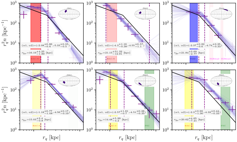
Figure 6: The radial density profile for several patches in the Galactocentric sky covering an area of $859.44\,{\rm deg}^{2}$. The purple crosses correspond to the radial densities of the highlighted region shown in the Mollweide map of each panel. The purple solid lines correspond to the double power law fit using 100 samples drawn from the parameters’ posterior distribution, and the dashed vertical lines correspond to the 16th and 84th percentiles of the $r_{br}$ posterior distribution. The black solid line is the best fit performed on the whole LSDR9 footprint. Each panel also shows the contribution of known substructures in a given region: HAC-N (red), VOD (blue), HAC-S (yellow), Pisces (green) and Sgr stream (pink). The darker the highlighted region is, the stronger the contribution of the substructure on the highlighted Galactocentric region.

Figure 6 shows the strength of the methodology developed in Section 3.1. By assigning a probabilistic BHB number for a given direction, we have a more detailed stellar halo profile compared to previous studies and can study any angular difference between the profiles. A similar approach was done by Hernitschek et al. (2018) as they probed the halo in several slices in $(l,b)$. However, they sliced in patches which cover an area in the sky almost twice as large as the ones depicted here, removed HAC and VOD overdensities, and excluded the inner parts of the Galaxy, $r_{q}<20$ kpc. We now detail the features in those regions which include the known overdensities.

The top left and middle panels in Figure 6 show the density profile of two patches which include the HAC-N overdensity, as defined by the coordinates given in Table 1. The former contains most of the overdensity, as highlighted by the darker red band compared to the latter, and its profile shows a clear break radius at $r<20$ kpc. At larger radii, the profile has a steeper decrease compared to the average LSDR9, but we note that the last two radial bins have a large uncertainty. On the other hand, the radial profile of the patch shown in the middle panel is consistent with a single power law and also shows an overall underdensity at radii greater than 20 kpc.

The top right panel in Figure 6 shows one of the sky patches that includes VOD. In this direction, the Sgr leading and trailing arms are expected to contribute at $r_{q}\approx 35$ kpc and $r_{q}\approx 60$ kpc, respectively, (as in Hernitschek et al. 2017). Although we have removed stars associated with Sgr (Section 2.3), there is still a slight overdensity at the distances associated with Sgr’s leading arm. Moreover, the overdensity associated with VOD seems to be at a slightly larger distance than what was previously reported, and closer to the break radius, i.e. at $r_{q}\approx$ 20 kpc.

The bottom row in Figure 6 shows the density profile in three patches of the Galactocentric sky which contain HAC-S and Pisces overdensities. In this coordinate system, they overlap in angular space, a feature which is missed in the Galactic coordinate system (see the top left panel in Figure 4). One can visualise it as being at the centre of the MW, looking towards a direction in the sky and seeing through two overdensities located at different radii. Firstly, the inner parts, located within the break radius, consistently show an overdensity associated with HAC-S. Secondly, the overdensity associated with Pisces seems to be mainly located in the patch centred at $\Phi_{gc}\approx 67.5$ deg and $\Theta_{gc}\approx-41.8$, and shown in the bottom right panel. This panel shows an overdensity through all radii, due to HAC-S and Pisces, and its outer slope is as steep as the average halo. These facts have implications on the interpretation of the possible origin scenarios of Pisces, as we will discuss in Section 5.

4.3 The anisotropy of the halo density profile

The anisotropy of the halo density profile is depicted in Figure 7. The top and middle panels show the inner and outer slopes, respectively, of the double power law model fit for regions shown in Figure 13. We only show the regions with more than four radial density bins available. The crosses indicate the patches where $|\alpha_{out}|-|\alpha_{in}|<1.5$, the orange-coloured pixels in the bottom panel. These patches do not show strong evidence for a broken power law profile, or the least their difference is lower than what is observed in the global profile.

The inner parts of the halo show significant differences in the profile across the Galactocentric sky, as indicated by $\alpha_{in}$. For instance, the regions associated with HAC-N, HAC-S and VOD have a flatter inner profile compared to the average LSDR9 profile, as indicated by the lighter-coloured pixels shown in the top panel, in contrast to most of the patches, except for regions in the fourth quadrant.

The regions marked with “x” indicate where $|\alpha_{out}|-|\alpha_{in}|>1.5$, white- to purple-coloured pixels in the bottom panel, but the error in the break radius is larger than 25%. Interestingly, this is observed in the regions where HAC-S and Pisces regions overlap (as shown in Figure 6), whereas the patch which includes only Pisces does not show evidence of a broken profile. The other three patches with significant differences between inner and outer profiles, but with $r_{br}$ poorly constrained, are either close to the Galactocentric plane, or near Sgr stream or LMC stellar halo contaminants.

Recently, Medina et al. (2024) showed how the density profile varies for four small patches, area $\lesssim 80\,{\deg}^{2}$, in the sky. They also highlighted the dependence of the halo density profile on the regions probed by a survey and the stellar tracer used. The results presented here do confirm significant differences in the stratified stellar halo, for rather larger sky patches, when compared to the global average. This has not been shown previously, as most studies either focused on a particular patch of the sky or did not probe the halo with a similar Galactocentric radial extent as done here.

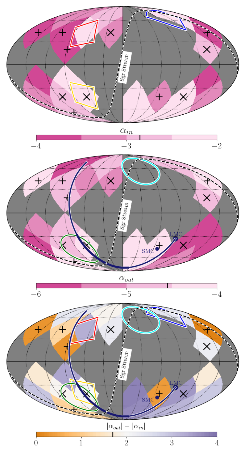
Figure 7: Mollweide projection of the Galactocentric coordinates $(\Phi_{gc},\Theta_{gc})$. The projection is divided into a grid of 48 pixels ($nside=2$) with equal area. The blue, red, yellow and orange regions delineate the regions associated with VOD, HAC-N, HAC-S and Pisces at their typical distances. Top panel: The inner slope, $\alpha_{in}$, measured at $r_{q}=15$ kpc, of the two power law model. Middle panel: The outer slope, $\alpha_{out}$, measured at $r_{q}=50$ kpc, of the two power law model. Bottom panel: The difference between $\alpha_{in}$ and $\alpha_{out}$. These panels highlight the anisotropy of the MW stellar halo profile, where several patches of the sky have distinct slopes compared to the average halo. We only show patches with more than four density points in the radial binning. The crosses and “x” indicate the regions with $|\alpha_{out}|-|\alpha_{in}|<1.5$, and $|\alpha_{out}|-|\alpha_{in}|>1.5$ with error in the break radius greater than 25%, respectively.

5 Discussion

In this current work, we found that the average density profile of the MW halo, as traced by the BHB stars, is described by a double power law (Figure 4, top right panel) corroborating with a plethora of similar studies. Medina et al. (2024) argues that the apparent lack of consensus on the exact profile shape, e.g. either single- or double power-law, can be understood by the tracer being used, the magnitude range available, and the spatial selection used, such as the minimum/maximum Galactocentric radius in the density profile construction. In addition to that, and most importantly, the discrepancy found in the literature is also caused by the heavily anisotropic halo shown here.

Overall, the studies which find evidence for a single power law profile do not cover the inner parts of the Galaxy, i.e. $r_{gc}\lesssim 20$ kpc. Those which include the inner halo, in general, do find evidence for a double-power law profile with outer slopes with an overall agreement with the slope of the single-power law studies.

In Section 4, we have shown evidence for a broken power law (BPL) density profile for the BHB stars in LSDR9 with a break radius at 20 kpc. The BPL profile is also observed when looking at the directions of HAC-N/S and VOD overdensities and in some patches in the Galactocentric sky. Moreover, we do find significant anisotropy in the inner and outer halo as several patches have distinct slopes, see Figures 7 and 14, where the latter also compares with slopes found in previous works. Moreover, some regions have a profile consistent with a single power law, e.g. in the direction of the Pisces overdensity.

We proceed and discuss how our results can shed light on the understanding of the structure of the stellar halo. We separate the discussion into two sections; in Section 5.1 we discuss the inner halo which is mainly associated with the GSE debris, $r_{gc}<20$ kpc, and in Section 5.2 we focus on the outer halo which hosts imprints of the LMC passage.

5.1 The inner halo and the GSE debris

Deason et al. (2013) made the connection between the presence of a broken profile and the merger history of the MW using Bullock & Johnston (2005) simulations. The break radius corresponds to the apocenter pile-up of the debris from a past massive merger. The inner part of the halo, within the break radius, is dominated by the debris of the main merger and thus has a less steep density profile compared to the outer parts, dominated by minor accretion events. As they observed this in the MW, they concluded the MW had gone through a main accretion event in its early stages. This was yet another strong evidence among others (e.g. Chiba & Beers 2000; Gilmore et al. 2002; Meza et al. 2005), of the GSE merger event later confirmed with Gaia data (Belokurov et al. 2018; Helmi et al. 2018; Haywood et al. 2018).

More recently and thanks to Gaia and large spectroscopic surveys, the halo density profile is also built with halo star candidates selected based on stellar chemistry and kinematics (Han et al. 2022; Yang et al. 2022; Lane et al. 2023). This methodology relies on the fact that the GSE debris is the major contributor to the stellar halo mass (e.g. Naidu et al. 2020). Intriguingly, this approach has also provided evidence for a doubly broken halo, i.e. a three-power law model, when selecting GSE star candidates chemically (Han et al. 2022) or with a metallicity-kinematic decomposition (Yang et al. 2022). Each break radii is associated with a pericenter passage of the GSE merger (Naidu et al. 2021).

Besides that, the GSE debris has been associated with HAC-N/S and VOD substructures. They have been shown to share similar dynamics Simion et al. (2019) and chemodynamical (Perottoni et al. 2022) signatures as the GSE near the Solar neighbourhood. In Section 4.1 we showed that these regions share a similar broken radial profile with $r_{br}\approx 20$ and similar inner and outer slopes, and a clear signature of the overdensity in the inner parts, where these substructures have been identified. In Section 4.2 we further explored these regions in smaller patches in the Galactocentric sky reinforcing the signature of the overdensities.

The density profile for these specific overdensity regions associated with the GSE merger serves as a constraint to idealised simulations that mimic this merger event. For instance, Naidu et al. (2021) presented an N-body model, without gas and star formation, which reproduces several properties of the observed GSE debris, including HAC-S and VOD overdensities, but does not reproduce the substructure in the HAC-N region. The latter is also an important constraint, and its overdensity is also observed in previous studies (e.g. Huang & Koposov 2022), due to its similarity with HAC-S and VOD. In simulations with gas and star formation, either tailored (Amarante et al. 2022) or in fully cosmological context (Orkney et al. 2023), the debris of GSE-like mergers fully phase mixes in the inner parts after a few Gyr and do not show evidence for clear overdensities like HAC-N/S and VOD.

To complicate matters further, Orkney et al. (2023) has also shown evidence that MW-like galaxies in the Auriga simulations (Grand et al. 2017) can have stellar halos with high radial velocity anisotropy, i.e. like the GSE component in the MW, being built with up to three main dwarf satellites of similar mass. These accreted stars have enough similarity in chemistry and dynamical space making it almost impossible to distinguish them apart solely on [Fe/H], [$\alpha$/Fe], and with dynamics.

It remains to be seen, whether the presence of the HAC-N, HAC-S and VOD can be indeed a feature of a unique merger event which happened 10 Gyrs ago, or if any of these overdensities are indeed signatures of a more recent merger as argued by Donlon et al. (2020, 2023).

5.2 The outer halo and the LMC wake

To have a general picture of the outer halo, we divided the Galactocentric sphere into 192 equal-sized area pixels, using healpy Python package with HEALPIX pixelisation $nside=4$, and calculated the halo density at $50<r_{q}/{\rm kpc}<120$ using the methodology described in Section 3.1. We then calculate the density contrast and show it in Figure 8. The LMC past trajectory is shown as the purple line (Vasiliev 2023), with the thicker part corresponding to the orbit within the distance range shown in the map.

Although we removed stars within 12.5 degrees from the LMC centre, there is still an overdensity seen in the pixels surrounding LMC’s current position. These are likely contaminants of LMC star members, as the LMC stellar halo can extend up to 30 degrees from the LMC as seen with BHB stars (Belokurov & Koposov 2016) and RR Lyrae (Petersen et al. 2022).

It is also evident from Figure 8 the presence of regions with several regions with a density contrast close to $-1$. Due to the steep density profile at these distances, $\alpha_{out}=-4.55$, the average density is dominated by the regions with overdensities. In fact, $\sim 55\%$ of the BHB stars, as estimated with our methodology, is within $\sim 20\%$ of the pixels. If the BHB stars followed a purely Poisson distribution, the same amount of stars would be within $\sim 40\%$ of the pixels. This reinforces the highly anisotropic stellar halo of the MW being dominated by a few patches with overdensities.

The Pisces overdensity, as highlighted approximately by the green circle in Figure 8, has been recently associated with the transient dark matter wake caused by the LMC passage. Its signature has been associated with an overdensity of RR Lyrae (Belokurov et al. 2019) and K-giant stars (Conroy et al. 2021), and is now also observed with the probabilistic BHB star mapping developed in this work. This transient response of MW’s (dark) halo to the LMC is akin to the Chandrasekhar dynamical friction wake (Chandrasekhar 1943) and traces the orbital path of the LMC in the halo at large distances (e.g. Garavito-Camargo et al. 2019). The shape of this transient wake signal should also be proportional to the mass and velocity of the LMC (and the DM density of the ambient medium). Our BHB stars map can thus be used to measure the extent of the transient wake response. To this end, we study the BHB star density variations along the sky patches crossed by the LMC’s past orbit from Vasiliev (2023)) for $50<r/{\rm kpc}<120$.

The top and bottom panels of Figure 9 show how the density varies along the Magellanic Stream Coordinates (Nidever et al. 2008). For this exercise, we coarsened the angular resolution, compared to Figure 8, to reduce the Poisson noise. Despite the relatively large patches, it clearly shows the density peak at the Pisces region, point $B_{1}$, and how it decreases going further away in $L_{MS}$ and $B_{MS}$. From Figure 9, we can see that the Pisces overdensity is observed on a scale of 60 degrees along and 25 degrees across the LMC’s orbit, which would correspond to a wake width of $\sim 32$ kpc at $\sim 70$ kpc. Future density profile maps along the orbital path of the LMC, as those shown in Figure 9, to characterise the transient wake signal will help further constrain models of the MW-LMC interaction and provide an important test for the nature of dark matter on Galactic scales. We note in passing that the Pisces overdensity region may also overlap with the Magellanic Stellar Stream (MSS, Chandra et al. 2023a) and kinematics together with chemical abundance information could help disentangle the MSS from the wake of the LMC.

Simulations of the MW-LMC interaction also predict the barycenter shift of the MW-LMC system (e.g. Gómez et al. 2015; Garavito-Camargo et al. 2019), i.e. the gravitational collective response or “global wake”. This effect has been observed kinematically (Erkal et al. 2021; Petersen & Peñarrubia 2021) and the density dipole associated with the collective response (Weinberg 1998; Laporte et al. 2018a; Petersen & Peñarrubia 2020) should also, in principle, be observed in star counts (Garavito-Camargo et al. 2019). Recently, Conroy et al. (2021) have reported a possible detection of this signal using K giant stars. Given that BHBs come in greater numbers, we attempt to measure the signal from the dipole in star counts.

We show in Figure 8 the approximate region in the Galactocentric sky of the region defined by Conroy et al. (2021), magenta dashed-line, which we refer to as the Northern overdensity. The BHB density contrast map shows no apparent significant overdensity in this region, but there is an overdensity just to the north of the Northern overdensity. Part of this region is located in the region associated with OVO, indicated by the cyan circle, and relatively close to the Sgr Stream, the latter being mostly removed. Nonetheless, this may be the remains of Sgr at very large distances (e.g Sesar et al. 2017b).

Figure 10 shows the total density contrast measured in the Pisces overdensity region and the Northern overdensity which are associated with the transient and global wake respectively. The purple contours show the interquartile of the density contrast measured obtained from the posteriors of the density estimation. While Pisces overdensity shows a clear signature where the density contrast is $>0.6$, the signal measured in the Northern overdensity has a large error and is consistent with being negligible. While the dipole signal most certainly exists in stellar density, the current BHB star data falls short of making a statistically meaningful measurement of this signal. This may need to await tracers that come in larger numbers in order to detect this signal, e.g. Main Sequence Turn Off stars.

We also show the results predicted from Garavito-Camargo et al. (2019) simulations which have significantly lower signatures in the density map. This can be caused by the fact that their stellar halo started as a smooth component and in the MW the stellar halo is heterogeneous and thus the LMC can enhance some previously existing overdensity(ies). Indeed as shown in this study and others (e.g. Bell et al. 2008), the stellar halo beyond 50 kpc is not smooth but inhabited by substructure which due to the long orbital timescales have not had time to fully phase mix over a Hubble time (e.g. Johnston et al. 2008).

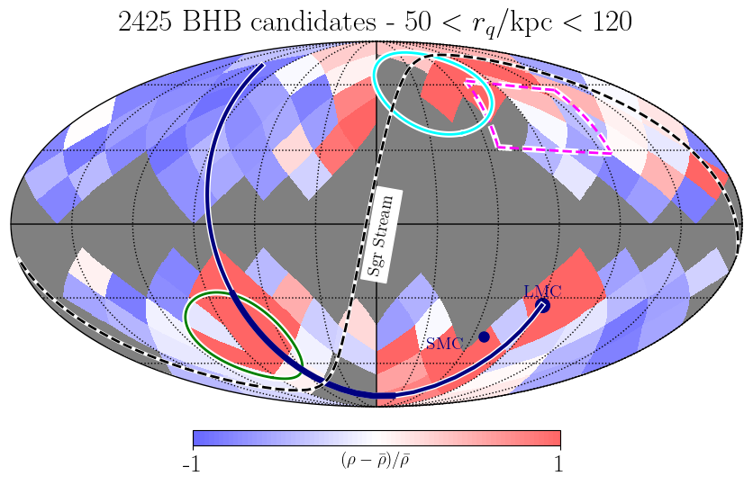
Figure 8: Density contrast of MW BHB stars in the stellar halo at $50<r_{q}/{\rm kpc}<120$ seen in Galactocentric coordinates $(\phi_{gc},\theta_{gc})$. The Mollweide projection is divided into a grid of 192 pixels ($nside=4$) with equal area. We delineate the approximate Galactocentric regions associated with OVO, Pisces, and Northern overdensity as the cyan, green, and magenta lines, respectively. The present-day position of the LMC and SMC are shown as the purple scatter points. LMC’s past trajectory (see Vasiliev 2023 for details) and Sgr stream are represented by the solid purple and dashed black lines, respectively.

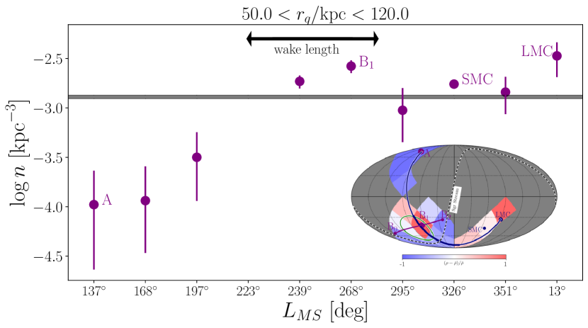
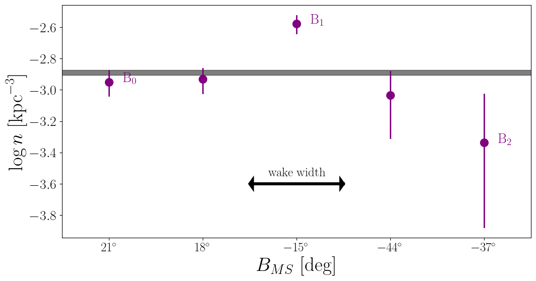
Figure 9: The BHB star density of the sky patches crossed by the LMC’s past orbit (Vasiliev 2023) as a function of the $(L_{MS},B_{MS})$ coordinates (Nidever et al. 2008). Each patch has an equal projected area of 859.44 ${\rm deg}^{2}$ (healpy using $nside=2$) and the density is calculated within $50<r/{\rm kpc}<120$. The 16th-84th percentiles of the average BHB density within this distance is shown by the shaded green line. Top panel: The density profile along LMC’s orbit from point $A$ to the pixel containing LMC. At $B_{1}$, the pixel dominated by Pisces overdensity, shows a clear signature of the overdensity in contrast to regions further away from it at $L_{MS}<230^{\circ}$. Bottom panel: The density profile as a function of $B_{MS}$ from point $B_{0}$ to $B_{1}$. At these large distances, and due to the steepness of the profile, the average density is dominated by the regions with the overdensities as illustrated in both panels.

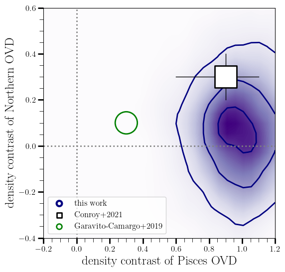
Figure 10: The BHB density contrast at $50<r_{q}/{\rm kpc}<120$ in the Pisces overdensity and the Northen overdensity regions, which are associated with the local wake and the collective response to the LMC orbit respectively. The purple contours to the shaded region correspond to the 16th, 50th and 84th confidence intervals calculated from the BHB fraction posteriors (see text for details). This result can not confirm the collective response of the MW stellar halo to the LMC passage. For comparison, we show previous measurements using K giant stars (Conroy et al. 2021) and predictions from MW-LMC interaction models (Garavito-Camargo et al. 2019).

6 Conclusion

We used LSDR9 photometric survey to study the density profile of the MW stellar halo. We developed a novel approach to modelling the $g-r$ and $r-z$ colour distribution allowing us to compute the fraction of BHB stars at any given direction. With this approach, we can robustly estimate the errors of the densities. We summarise our main results when probing the stellar halo within $5<r_{q}/{\rm kpc}<120$:

• The global stellar halo shows a broken power law density profile with inner and outer slopes, and break radius, $\alpha_{in}=-2.45^{+0.17}_{-0.14}$, $\alpha_{in}=-4.55^{+0.11}_{-0.1}$, $r_{br}=19.15^{+1.7}_{-1.8}$ kpc, respectively;

• HAC-S, HAC-N and VOD Galactic structures show a significant break in stellar density profiles at $r_{q}\approx 20$ kpc, with compatible density inner slopes (Figure 4). The presence of these three overdensities regions remains to be seen in tailored GSE-like merger models;

• The Pisces overdensity region is the only region where we see a density profile consistent with a single power law, in contrast to the previously mentioned overdensity regions;

• Even after excluding regions containing major overdensities we observe a density profile with a break which seems to indicate that the GSE debris is present in most directions in the Galaxy;

• We find strong evidence for an anisotropic stellar halo, indicated by significant differences in the steepness of the density profile when looking at different Galactocentric patches (Figure 7) and by $\sim 20\%$ of the sky containing $\sim 55\%$ of BHB stars at $r>50$ kpc (Section 5.2);

• The Pisces overdensity spans 60 degrees along and 25 degrees across the LMC’s orbital path in the sky (Figure 9);

• If thought to be associated with the transient wake response of the MW to the LMC, then the Pisces overdensity extension would correspond to a wake width of $\sim 32$ kpc at $\sim 70$ kpc (Section 5.2). Such a measurement may help set constraints on the mass and models of the MW-LMC system and also on the nature of dark matter;

• While we confirm the overdensity in the Pisces region, associated with the local wake induced by the LMC passage, our results do not show a statistically significant signature of the collective response in density (Figure 10).

The methodology developed in this work is a prelude to what will be possible with forthcoming photometric surveys such as the Chinese Space Station Telescope wide imaging survey (CSST, Zhan 2011; Cao et al. 2018), the Large Synoptic Survey Telescope (LSST, LSST Dark Energy Science Collaboration 2012), and Euclid space-based survey (Laureijs & et al. 2011). CSST will cover 17,500 ${\rm deg}^{2}$ ($\approx 40\%$ of the sky), observe in the $NUV$,$ugriz$ photometric bands, reaching a limiting magnitude of $r\approx 26.0$ and $r\approx 27.2$ for the wide and deep imaging survey (Qu et al. 2023), respectively. LSST main survey will cover 30,000 ${\rm deg}^{2}$ and reach up to $r\approx 27.5$ at the end of its mission. The depth to be reached by these surveys, with lower magnitude errors compared to LSDR9, will allow us to probe the stellar halo fraction at a higher spatial angular resolution and larger distances. This will refine the measurement of the gravitational wake width in the MW halo due to the LMC, as shown in Figure 9, particularly when extending this work’s methodology to Main Sequence Turn Off stars. These stars are not only more numerous than BHB stars (e.g. Bell et al. 2010), but they will reduce the Poisson noise and allow for finer measurements of density variations across/along the wake and across overdensities (Sanderson et al. 2019).

Finally, we present in Appendix C a catalogue of BHB star candidates with their respective probabilities calculated from Equation 3.

Appendix A White dwarf contamination

In this section, we investigate the possible white dwarf contamination in identifying BHB stars through our methodology described in Section 2.2.

We use the Gaia EDR3 white dwarf catalogue (Gentile Fusillo et al. 2021) to verify whether this stellar population could contaminate the BHB fraction estimation. As we are not interested in the purity of a white dwarf sample, but rather its contamination, we used all their white dwarf candidates to crossmatch with our LSDR9 sample. The left column in Figure 11 shows the $grz-(g-r)$ plane, at different $g$ intervals, the white dwarf candidates. The black rectangle highlights the region of interest in our study and in the right column, we show the $grz$ histogram, in light blue, for the objects inside it. We also show, in blue, the histogram for all star objects excluding the white dwarfs, that lie inside the selected region. The solid blue line is the histogram of all objects in the selected $grz-(g-r)$ region. It is clear that for $g>17$ there is a low contamination fraction of white dwarf candidates in the expected BHB region.

We verify the effect of not excluding white dwarf candidates on the BHB fraction estimation by fitting the $grz$ distribution for several intervals in $13<g<21$. We use the same methodology described in Section 3.1 and also include strong prior in the BHB Gaussian parameters. Figure 12 shows the fractions for the BHB, BS and background components in blue, orange and magenta, respectively. The dark/light markers exclude/include white dwarf candidates. We can see that the BHB fraction is independent of the removal or not of white dwarf candidates, at least in the color-color regime of our study. The most noticeable effect is on the BS and background contamination. We, therefore, verify that white dwarfs are not significant sources of contamination in our study.

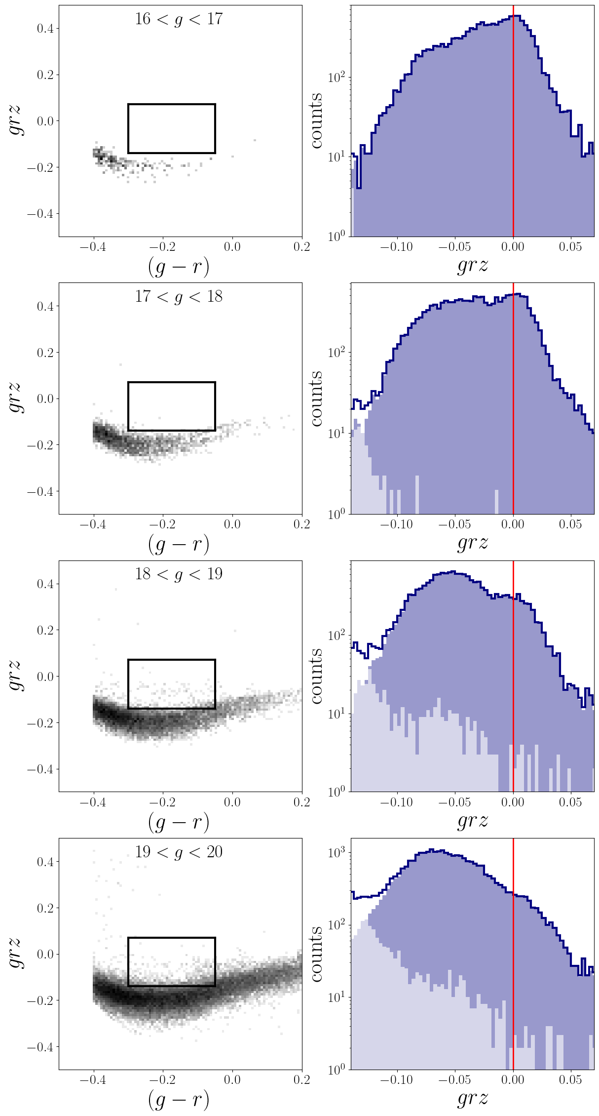
Figure 11: Left column: The $grz-(g-r)$ plane for the white dwarf stars in from the Gaia EDR3 catalogue (Gentile Fusillo et al. 2021). The black rectangle shows the region of interest in our study. Right column: The $grz$ histogram for objects inside the black rectangle. The white dwarf and non-white dwarf objects histograms are shown as the light and dark blue histograms, respectively. The solid blue line corresponds to their sum. The solid red line marks $grz=0$, the centre of the BHB distribution.

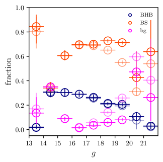
Figure 12: The fractions of each component from the MCMC modelling, described in Section 3.1, for objects with $-0.3<(g-r)<-0.05$ and $-0.14<grz<0.07$ in the LSDR9-Gaia EDR3 crossmatch. The BHB Gaussian component has a hard prior for the mean and standard deviation. The dark/light markers are the fractions for a given $g$ interval when white dwarf candidates are excluded/included. The white dwarf contamination in the BHB fractions is negligible throughout $g$.

Appendix B Radial density profiles

In Section 4.2, we divided the Galactocentric sky into 48 patches with the Python package healpy (Górski et al. 2005; Zonca et al. 2019) using $nside=2$. Each region has an equal projected area of 859.44 ${\rm deg}^{2}$. We constructed the density profiles, see Section 3 for details, for 10 bins equally space in logarithm in the range $5<r_{q}/{\rm kpc}<120$. Figure 13 shows the profiles of all the patches which have four or more bins in $r_{q}$.

Figure 14 shows the inner and outer slopes, from the broken-power law fitting (see Section 3.3) for each patch of the Galactocentric sky with four or more radial bins. The coordinates of the centre of each patch are given on the x-axis in degrees. The panel highlights the highly anisotropic stellar halo, as observed with BHB stars and discussed throughout in Section 5. We also show the slopes obtained by several studies as compiled by Yu et al. (2024).

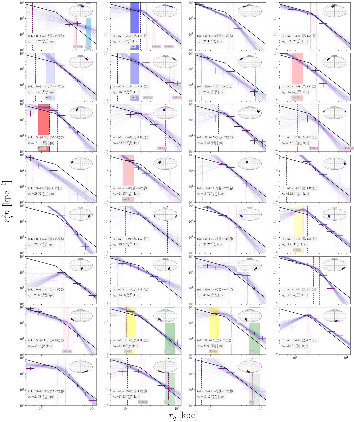
Figure 13: Radial density profiles for several patches in the Galactocentric sky as in Figure 6. We show all the regions with more than four radial bins. See Section 4.2 for details.

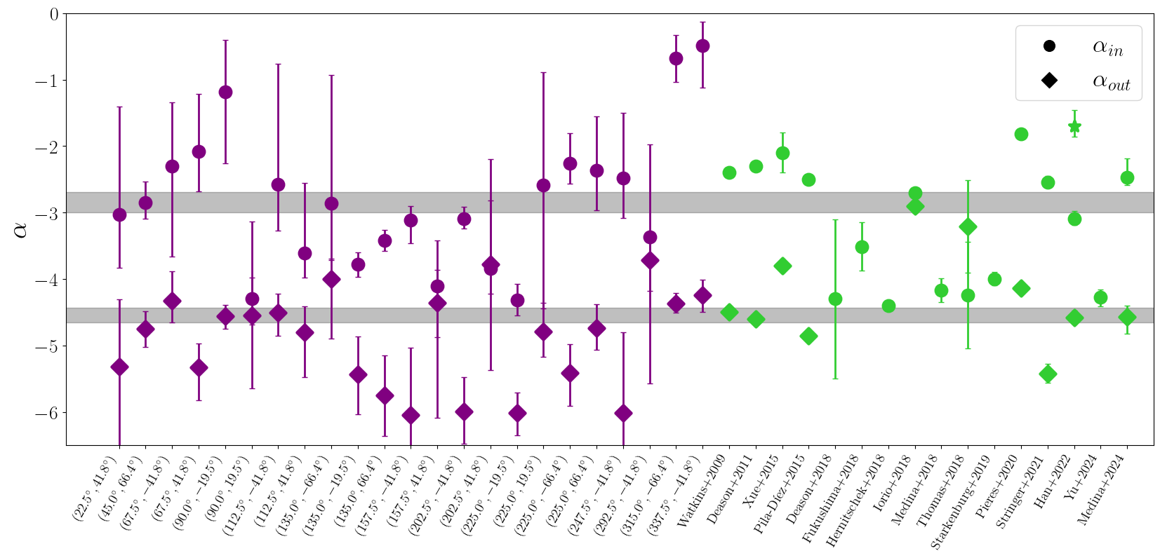
Figure 14: The inner (outer) slopes of the broken power law model fit of the density profiles shown in Figure 13 shown as purple square (diamond) markers. The x-axis shows the coordinates in degrees of the centre of the Galactocentric patch using healpy Python package with HEALPIX pixelisation $nside=2$. The shaded region corresponds to the slopes measured for the average radial density profile as in Section 4.1. We also included the list compiled by Yu et al. (2024) of several works studying the halo radial density profile: Watkins et al. (2009); Deason et al. (2011); Xue et al. (2015); Pila-Díez et al. (2015); Deason et al. (2018); Fukushima et al. (2018); Hernitschek et al. (2018); Iorio et al. (2018); Medina et al. (2018); Thomas et al. (2018); Starkenburg et al. (2019); Pieres et al. (2020); Stringer et al. (2021); Han et al. (2022); Yu et al. (2024); Medina et al. (2024). Han et al. (2022) favours a three-power-law model and thus the extra slope is shown as the star marker.

Appendix C LSDR9 BHB star candidates catalogue

We use objects from Legacy Survey Data Release 9 (Dey et al. 2019) with the colour selection of Equation 2. We then construct a catalogue with 95446 objects containing LSDR9 release, brickid and objid. These three parameters provide a unique identifier hash. The catalogue also includes R.A., Dec., the extinction corrected $g_{0}$, $r_{0}$, $z_{0}$, $grz$ (Equation 1), and the probability of a stellar object being a BHB star, $P_{BHB}$, calculated with Equation 3. Table 2 shows the header and first 10 rows of the catalogue and will be available online.

release	brickid	objid	R.A. [deg]	Dec [deg]	$g_{0}$	$r_{0}$	$z_{0}$	$grz$	$M_{g}$	$P_{BHB}$
9010	279546	378	211.46	-8.89	16.41	16.61	16.84	0.04	0.54	0.55
9010	279546	399	211.47	-8.88	19.04	19.22	19.49	-0.03	0.5	0.44
9010	282395	4350	211.54	-8.42	14.55	14.79	15.07	0.02	0.63	0.85
9010	282396	3890	211.75	-8.54	15.74	15.99	16.29	0.01	0.66	0.93
9010	283822	5900	211.79	-8.32	20.56	20.69	20.93	-0.05	0.46	0.15
9010	283819	817	210.84	-8.34	15.64	15.86	16.15	-0.0	0.58	0.91
9010	283819	3721	210.98	-8.33	16.21	16.28	16.48	-0.05	0.43	0.01
9010	285246	4170	210.96	-7.93	20.62	20.79	20.99	0.03	0.49	0.85
9010	286673	4635	210.73	-7.82	19.72	19.83	20.0	0.02	0.45	0.9
9010	286674	1976	210.85	-7.68	16.22	16.34	16.56	-0.01	0.46	0.77

Table 2: First 10 rows of the catalogue constructed with LSDR9 objects. See Appendix C for details.

References

- Amarante et al. (2022) Amarante, J. A. S., Debattista, V. P., Beraldo e Silva, L., Laporte, C. F. P., & Deg, N. 2022, ApJ, 937, 12
- Amarante et al. (2020) Amarante, J. A. S., Smith, M. C., & Boeche, C. 2020, MNRAS, 492, 3816
- Anders et al. (2021) Anders, F., Cantat-Gaudin, T., Quadrino-Lodoso, I., et al. 2021, A&A, 645, L2
- Barbosa et al. (2022) Barbosa, F. O., Santucci, R. M., Rossi, S., et al. 2022, ApJ, 940, 30
- Beers & Christlieb (2005) Beers, T. C. & Christlieb, N. 2005, ARA&A, 43, 531
- Bell et al. (2010) Bell, E. F., Xue, X. X., Rix, H.-W., Ruhland, C., & Hogg, D. W. 2010, AJ, 140, 1850
- Bell et al. (2008) Bell, E. F., Zucker, D. B., Belokurov, V., et al. 2008, ApJ, 680, 295
- Belokurov et al. (2019) Belokurov, V., Deason, A. J., Erkal, D., et al. 2019, MNRAS, 488, L47
- Belokurov et al. (2018) Belokurov, V., Erkal, D., Evans, N. W., Koposov, S. E., & Deason, A. J. 2018, MNRAS, 478, 611
- Belokurov et al. (2007a) Belokurov, V., Evans, N. W., Bell, E. F., et al. 2007a, ApJ, 657, L89
- Belokurov & Koposov (2016) Belokurov, V. & Koposov, S. E. 2016, MNRAS, 456, 602
- Belokurov et al. (2014) Belokurov, V., Koposov, S. E., Evans, N. W., et al. 2014, MNRAS, 437, 116
- Belokurov et al. (2007b) Belokurov, V., Zucker, D. B., Evans, N. W., et al. 2007b, ApJ, 654, 897
- Bennett & Bovy (2019) Bennett, M. & Bovy, J. 2019, MNRAS, 482, 1417
- Besla et al. (2007) Besla, G., Kallivayalil, N., Hernquist, L., et al. 2007, ApJ, 668, 949
- Bird et al. (2021) Bird, S. A., Xue, X.-X., Liu, C., et al. 2021, ApJ, 919, 66
- Bonaca et al. (2012) Bonaca, A., Jurić, M., Ivezić, Ž., et al. 2012, AJ, 143, 105
- Borbolato et al. (2023) Borbolato, L., Perottoni, H. D., Rossi, S., et al. 2023, arXiv e-prints, arXiv:2309.15321
- Brook et al. (2003) Brook, C. B., Kawata, D., Gibson, B. K., & Flynn, C. 2003, ApJ, 585, L125
- Bullock & Johnston (2005) Bullock, J. S. & Johnston, K. V. 2005, ApJ, 635, 931
- Cao et al. (2018) Cao, Y., Gong, Y., Meng, X.-M., et al. 2018, MNRAS, 480, 2178
- Carr et al. (2022) Carr, C., Johnston, K. V., Laporte, C. F. P., & Ness, M. K. 2022, MNRAS, 516, 5067
- Carrillo et al. (2024) Carrillo, A., Deason, A. J., Fattahi, A., Callingham, T. M., & Grand, R. J. J. 2024, MNRAS, 527, 2165
- Cerny et al. (2023) Cerny, W., Martínez-Vázquez, C. E., Drlica-Wagner, A., et al. 2023, ApJ, 953, 1
- Chandra et al. (2023a) Chandra, V., Naidu, R. P., Conroy, C., et al. 2023a, ApJ, 956, 110
- Chandra et al. (2023b) Chandra, V., Naidu, R. P., Conroy, C., et al. 2023b, ApJ, 951, 26
- Chandrasekhar (1943) Chandrasekhar, S. 1943, ApJ, 97, 255
- Chiba & Beers (2000) Chiba, M. & Beers, T. C. 2000, AJ, 119, 2843
- Conroy et al. (2021) Conroy, C., Naidu, R. P., Garavito-Camargo, N., et al. 2021, Nature, 592, 534
- Cunningham et al. (2020) Cunningham, E. C., Garavito-Camargo, N., Deason, A. J., et al. 2020, ApJ, 898, 4
- Das et al. (2020) Das, P., Hawkins, K., & Jofré, P. 2020, MNRAS, 493, 5195
- Deason et al. (2011) Deason, A. J., Belokurov, V., & Evans, N. W. 2011, MNRAS, 416, 2903
- Deason et al. (2013) Deason, A. J., Belokurov, V., Evans, N. W., & Johnston, K. V. 2013, ApJ, 763, 113
- Deason et al. (2018) Deason, A. J., Belokurov, V., & Koposov, S. E. 2018, ApJ, 852, 118
- Deason et al. (2014) Deason, A. J., Belokurov, V., Koposov, S. E., & Rockosi, C. M. 2014, ApJ, 787, 30
- Deason et al. (2019) Deason, A. J., Belokurov, V., & Sanders, J. L. 2019, MNRAS, 490, 3426
- Dey et al. (2019) Dey, A., Schlegel, D. J., Lang, D., et al. 2019, AJ, 157, 168
- Donlon et al. (2023) Donlon, Thomas, I., Newberg, H. J., Sanderson, R., et al. 2023, arXiv e-prints, arXiv:2310.09376
- Donlon et al. (2020) Donlon, Thomas, I., Newberg, H. J., Sanderson, R., & Widrow, L. M. 2020, ApJ, 902, 119
- Dotter et al. (2010) Dotter, A., Sarajedini, A., Anderson, J., et al. 2010, ApJ, 708, 698
- Erkal et al. (2021) Erkal, D., Deason, A. J., Belokurov, V., et al. 2021, MNRAS, 506, 2677
- Feuillet et al. (2020) Feuillet, D. K., Feltzing, S., Sahlholdt, C. L., & Casagrande, L. 2020, MNRAS, 497, 109
- Forbes (2020) Forbes, D. A. 2020, MNRAS, 493, 847
- Foreman-Mackey et al. (2013) Foreman-Mackey, D., Hogg, D. W., Lang, D., & Goodman, J. 2013, PASP, 125, 306
- Frebel & Norris (2015) Frebel, A. & Norris, J. E. 2015, ARA&A, 53, 631
- Fukushima et al. (2018) Fukushima, T., Chiba, M., Homma, D., et al. 2018, PASJ, 70, 69
- Fukushima et al. (2019) Fukushima, T., Chiba, M., Tanaka, M., et al. 2019, PASJ, 71, 72
- Gallart et al. (2019) Gallart, C., Bernard, E. J., Brook, C. B., et al. 2019, Nature Astronomy, 3, 932
- Garavito-Camargo et al. (2019) Garavito-Camargo, N., Besla, G., Laporte, C. F. P., et al. 2019, ApJ, 884, 51
- Garavito-Camargo et al. (2021) Garavito-Camargo, N., Patel, E., Besla, G., et al. 2021, ApJ, 923, 140
- Gentile Fusillo et al. (2021) Gentile Fusillo, N. P., Tremblay, P. E., Cukanovaite, E., et al. 2021, MNRAS, 508, 3877
- Gilmore et al. (2002) Gilmore, G., Wyse, R. F. G., & Norris, J. E. 2002, ApJ, 574, L39
- Gómez et al. (2015) Gómez, F. A., Besla, G., Carpintero, D. D., et al. 2015, ApJ, 802, 128
- Gómez et al. (2013) Gómez, F. A., Minchev, I., O’Shea, B. W., et al. 2013, MNRAS, 429, 159
- Górski et al. (2005) Górski, K. M., Hivon, E., Banday, A. J., et al. 2005, ApJ, 622, 759
- Grand et al. (2017) Grand, R. J. J., Gómez, F. A., Marinacci, F., et al. 2017, MNRAS, 467, 179
- Han et al. (2022) Han, J. J., Conroy, C., Johnson, B. D., et al. 2022, arXiv e-prints, arXiv:2208.04327
- Haywood et al. (2018) Haywood, M., Di Matteo, P., Lehnert, M. D., et al. 2018, ApJ, 863, 113
- Helmi et al. (2018) Helmi, A., Babusiaux, C., Koppelman, H. H., et al. 2018, Nature, 563, 85
- Helmi et al. (1999) Helmi, A., White, S. D. M., de Zeeuw, P. T., & Zhao, H. 1999, Nature, 402, 53
- Hernitschek et al. (2018) Hernitschek, N., Cohen, J. G., Rix, H.-W., et al. 2018, ApJ, 859, 31
- Hernitschek et al. (2017) Hernitschek, N., Sesar, B., Rix, H.-W., et al. 2017, ApJ, 850, 96
- Huang & Koposov (2022) Huang, K.-W. & Koposov, S. E. 2022, MNRAS, 510, 3575
- Ibata et al. (1994) Ibata, R. A., Gilmore, G., & Irwin, M. J. 1994, Nature, 370, 194
- Iorio et al. (2018) Iorio, G., Belokurov, V., Erkal, D., et al. 2018, MNRAS, 474, 2142
- Johnston et al. (2008) Johnston, K. V., Bullock, J. S., Sharma, S., et al. 2008, ApJ, 689, 936
- Johnston et al. (1995) Johnston, K. V., Spergel, D. N., & Hernquist, L. 1995, ApJ, 451, 598
- Jurić et al. (2008) Jurić, M., Ivezić, Ž., Brooks, A., et al. 2008, ApJ, 673, 864
- Kollmeier et al. (2009) Kollmeier, J. A., Gould, A., Shectman, S., et al. 2009, ApJ, 705, L158
- Koposov et al. (2015) Koposov, S. E., Belokurov, V., Torrealba, G., & Evans, N. W. 2015, ApJ, 805, 130
- Koppelman et al. (2019) Koppelman, H. H., Helmi, A., Massari, D., Price-Whelan, A. M., & Starkenburg, T. K. 2019, A&A, 631, L9
- Lane et al. (2023) Lane, J. M. M., Bovy, J., & Mackereth, J. T. 2023, MNRAS, 526, 1209
- Laporte et al. (2018a) Laporte, C. F. P., Gómez, F. A., Besla, G., Johnston, K. V., & Garavito-Camargo, N. 2018a, MNRAS, 473, 1218
- Laporte et al. (2018b) Laporte, C. F. P., Johnston, K. V., Gómez, F. A., Garavito-Camargo, N., & Besla, G. 2018b, MNRAS, 481, 286
- Laporte et al. (2019) Laporte, C. F. P., Minchev, I., Johnston, K. V., & Gómez, F. A. 2019, MNRAS, 485, 3134
- Laureijs & et al. (2011) Laureijs, R. & et al. 2011, arXiv e-prints, arXiv:1110.3193
- Li et al. (2019) Li, T. S., Koposov, S. E., Zucker, D. B., et al. 2019, MNRAS, 490, 3508
- Limberg et al. (2021) Limberg, G., Rossi, S., Beers, T. C., et al. 2021, ApJ, 907, 10
- Limberg et al. (2022) Limberg, G., Souza, S. O., Pérez-Villegas, A., et al. 2022, ApJ, 935, 109
- Liu et al. (2022) Liu, G., Huang, Y., Bird, S. A., et al. 2022, MNRAS, 517, 2787
- LSST Dark Energy Science Collaboration (2012) LSST Dark Energy Science Collaboration. 2012, arXiv e-prints, arXiv:1211.0310
- Malhan et al. (2022) Malhan, K., Ibata, R. A., Sharma, S., et al. 2022, arXiv e-prints, arXiv:2202.07660
- Massari et al. (2019) Massari, D., Koppelman, H. H., & Helmi, A. 2019, A&A, 630, L4
- McConnachie (2012) McConnachie, A. W. 2012, AJ, 144, 4
- McMillan (2017) McMillan, P. J. 2017, MNRAS, 465, 76
- Medina et al. (2024) Medina, G. E., Muñoz, R. R., Carlin, J. L., et al. 2024, arXiv e-prints, arXiv:2402.14055
- Medina et al. (2018) Medina, G. E., Muñoz, R. R., Vivas, A. K., et al. 2018, ApJ, 855, 43
- Meza et al. (2005) Meza, A., Navarro, J. F., Abadi, M. G., & Steinmetz, M. 2005, MNRAS, 359, 93
- Montalbán et al. (2021) Montalbán, J., Mackereth, J. T., Miglio, A., et al. 2021, Nature Astronomy, 5, 640
- Myeong et al. (2018) Myeong, G. C., Evans, N. W., Belokurov, V., Sanders, J. L., & Koposov, S. E. 2018, ApJ, 863, L28
- Naidu et al. (2020) Naidu, R. P., Conroy, C., Bonaca, A., et al. 2020, ApJ, 901, 48
- Naidu et al. (2021) Naidu, R. P., Conroy, C., Bonaca, A., et al. 2021, ApJ, 923, 92
- Newberg et al. (2002) Newberg, H. J., Yanny, B., Rockosi, C., et al. 2002, ApJ, 569, 245
- Nidever et al. (2008) Nidever, D. L., Majewski, S. R., & Burton, W. B. 2008, in Astrophysics and Space Science Proceedings, Vol. 5, Galaxies in the Local Volume, 243
- Nie et al. (2015) Nie, J. D., Smith, M. C., Belokurov, V., et al. 2015, ApJ, 810, 153
- Orkney et al. (2023) Orkney, M. D. A., Laporte, C. F. P., Grand, R. J. J., et al. 2023, MNRAS, 525, 683
- Pace et al. (2022) Pace, A. B., Erkal, D., & Li, T. S. 2022, ApJ, 940, 136
- Perottoni et al. (2022) Perottoni, H. D., Limberg, G., Amarante, J. A. S., et al. 2022, ApJ, 936, L2
- Petersen & Peñarrubia (2020) Petersen, M. S. & Peñarrubia, J. 2020, MNRAS, 494, L11
- Petersen & Peñarrubia (2021) Petersen, M. S. & Peñarrubia, J. 2021, Nature Astronomy, 5, 251
- Petersen et al. (2022) Petersen, M. S., Peñarrubia, J., & Jones, E. 2022, MNRAS, 514, 1266
- Pieres et al. (2020) Pieres, A., Girardi, L., Balbinot, E., et al. 2020, MNRAS, 497, 1547
- Pila-Díez et al. (2015) Pila-Díez, B., de Jong, J. T. A., Kuijken, K., van der Burg, R. F. J., & Hoekstra, H. 2015, A&A, 579, A38
- Purcell et al. (2011) Purcell, C. W., Bullock, J. S., Tollerud, E. J., Rocha, M., & Chakrabarti, S. 2011, Nature, 477, 301
- Qu et al. (2023) Qu, H., Yuan, Z., Doliva-Dolinsky, A., et al. 2023, MNRAS, 523, 876
- Ross et al. (2012) Ross, N. P., Myers, A. D., Sheldon, E. S., et al. 2012, ApJS, 199, 3
- Sanderson et al. (2019) Sanderson, R., Carlin, J., Cunningham, E., et al. 2019, BAAS, 51, 347
- Santucci et al. (2015) Santucci, R. M., Beers, T. C., Placco, V. M., et al. 2015, ApJ, 813, L16
- Schlegel et al. (1998) Schlegel, D. J., Finkbeiner, D. P., & Davis, M. 1998, ApJ, 500, 525
- Searle & Zinn (1978) Searle, L. & Zinn, R. 1978, ApJ, 225, 357
- Sesar et al. (2017a) Sesar, B., Hernitschek, N., Dierickx, M. I. P., Fardal, M. A., & Rix, H.-W. 2017a, ApJ, 844, L4
- Sesar et al. (2017b) Sesar, B., Hernitschek, N., Mitrović, S., et al. 2017b, AJ, 153, 204
- Sesar et al. (2010) Sesar, B., Ivezić, Ž., Grammer, S. H., et al. 2010, ApJ, 708, 717
- Sesar et al. (2007) Sesar, B., Ivezić, Ž., Lupton, R. H., et al. 2007, AJ, 134, 2236
- Simion et al. (2014) Simion, I. T., Belokurov, V., Irwin, M., & Koposov, S. E. 2014, MNRAS, 440, 161
- Simion et al. (2019) Simion, I. T., Belokurov, V., & Koposov, S. E. 2019, MNRAS, 482, 921
- Sirko et al. (2004) Sirko, E., Goodman, J., Knapp, G. R., et al. 2004, AJ, 127, 899
- Springel et al. (2006) Springel, V., Frenk, C. S., & White, S. D. M. 2006, Nature, 440, 1137
- Starkenburg et al. (2019) Starkenburg, E., Youakim, K., Martin, N., et al. 2019, MNRAS, 490, 5757
- Stringer et al. (2021) Stringer, K. M., Drlica-Wagner, A., Macri, L., et al. 2021, ApJ, 911, 109
- Thomas et al. (2018) Thomas, G. F., McConnachie, A. W., Ibata, R. A., et al. 2018, MNRAS, 481, 5223
- Vasiliev (2019) Vasiliev, E. 2019, MNRAS, 482, 1525
- Vasiliev (2023) Vasiliev, E. 2023, Galaxies, 11, 59
- Vickers et al. (2012) Vickers, J. J., Grebel, E. K., & Huxor, A. P. 2012, AJ, 143, 86
- Vivas et al. (2001) Vivas, A. K., Zinn, R., Andrews, P., et al. 2001, ApJ, 554, L33
- Watkins et al. (2009) Watkins, L. L., Evans, N. W., Belokurov, V., et al. 2009, MNRAS, 398, 1757
- Weinberg (1989) Weinberg, M. D. 1989, MNRAS, 239, 549
- Weinberg (1998) Weinberg, M. D. 1998, MNRAS, 299, 499
- Weinberg & Blitz (2006) Weinberg, M. D. & Blitz, L. 2006, ApJ, 641, L33
- White & Frenk (1991) White, S. D. M. & Frenk, C. S. 1991, ApJ, 379, 52
- Wright et al. (2010) Wright, E. L., Eisenhardt, P. R. M., Mainzer, A. K., et al. 2010, AJ, 140, 1868
- Wu et al. (2022a) Wu, W., Zhao, G., Xue, X.-X., Bird, S. A., & Yang, C. 2022a, ApJ, 924, 23
- Wu et al. (2022b) Wu, W., Zhao, G., Xue, X.-X., Pei, W., & Yang, C. 2022b, AJ, 164, 41
- Xiang & Rix (2022) Xiang, M. & Rix, H.-W. 2022, Nature, 603, 599
- Xue et al. (2015) Xue, X.-X., Rix, H.-W., Ma, Z., et al. 2015, ApJ, 809, 144
- Xue et al. (2011) Xue, X.-X., Rix, H.-W., Yanny, B., et al. 2011, ApJ, 738, 79
- Yang et al. (2022) Yang, C., Zhu, L., Tahmasebzadeh, B., Xue, X.-X., & Liu, C. 2022, AJ, 164, 241
- Yanny et al. (2000) Yanny, B., Newberg, H. J., Kent, S., et al. 2000, ApJ, 540, 825
- Yu et al. (2024) Yu, F., Li, T. S., Speagle, J. S., et al. 2024, arXiv e-prints, arXiv:2402.00104
- Yuan et al. (2020) Yuan, Z., Myeong, G. C., Beers, T. C., et al. 2020, ApJ, 891, 39
- Zhan (2011) Zhan, H. 2011, Scientia Sinica Physica, Mechanica & Astronomica, 41, 1441
- Zhou et al. (2023) Zhou, R., Dey, A., Lang, D., et al. 2023, Research Notes of the American Astronomical Society, 7, 105
- Zonca et al. (2019) Zonca, A., Singer, L., Lenz, D., et al. 2019, Journal of Open Source Software, 4, 1298