Data-Driven Stability Assessment of Power Electronic Converters with Multi-Resolution Dynamic Mode Decomposition
Abstract
Harmonic instability occurs frequently in the power electronic converter system. This paper leverages multi-resolution dynamic mode decomposition (MR-DMD) as a data-driven diagnostic tool for the system stability of power electronic converters, not requiring complex modeling and detailed control information. By combining dynamic mode decomposition (DMD) with the multi-resolution analysis used in wavelet theory, dynamic modes and eigenvalues can be identified at different decomposition levels and time scales with the MR-DMD algorithm, thereby allowing for handling datasets with transient time behaviors, which is not achievable using conventional DMD. Further, the selection criteria for important parameters in MR-DMD are clearly defined through derivation, elucidating the reason for enabling it to extract eigenvalues within different frequency ranges. Finally, the analysis results are verified using the dataset collected from the experimental platform of a low-frequency oscillation scenario in electrified railways featuring a single-phase converter.
Index Terms:
Grid-tied converter, oscillation mode identification, dynamic mode decomposition, multi-resolution analysis.I Introduction
With the advent of modern power electronic-based power systems involving widespread applications of grid-tied power electronic converters, there are frequent occurrences of various small-signal stability issues across a wide frequency range [1]. There are two main analytical methods, i.e., eigenvalue analysis based on the state-space model [2] and the impedance-based analysis based on the transfer functions [3]. However, due to the complexity and limited controller information of modeling actual power electronic converter systems, data-driven mode identification techniques are more practical.
Regarding mode identification methods, Prony algorithm[4], Matrix Pencil algorithm[5], and eigensystem realization algorithm (ERA) [6] are reported and compared in [7], which can extract system eigenvalues to assess system stability intuitively. As a powerful data-driven tool originating from the field of fluid dynamics, dynamic mode decomposition (DMD) [8] can extract dynamic modes and eigenvalues for stability assessment by performing eigen-decomposition of the best fit dynamic matrix dimensionally reduced via singular value decomposition (SVD) [9]. With unique advantages in capturing spatio-temporal characteristics of data snapshots, DMD has been used for oscillation analysis in power systems [10], and it was demonstrated that DMD has clear physical significance and superior accuracy compared to the aforementioned three identification methods [10]. However, DMD performs global processing on all data within the sampling time window, which results in poor robustness to correctly identify transient time behaviors or outliers within the dataset such as stability state changing and missing data [11].
To address the aforementioned problems, an oscillation identification method based on multi-resolution dynamic mode decomposition (MR-DMD) [11] is presented in this paper. Dominant dynamic modes can be obtained in different frequency ranges and varying timescales for stability assessment. Then, selection criteria for the key parameters of MR-DMD are developed through rigorous mathematical derivations. The method performance and its advantages are demonstrated with an experimental dataset sampled from a single-phase converter platform when low-frequency oscillation occurs, but the proposed methodology is generic for wide frequency ranges.
II System Description amd Problem Formulation
II-A System Description
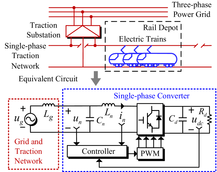
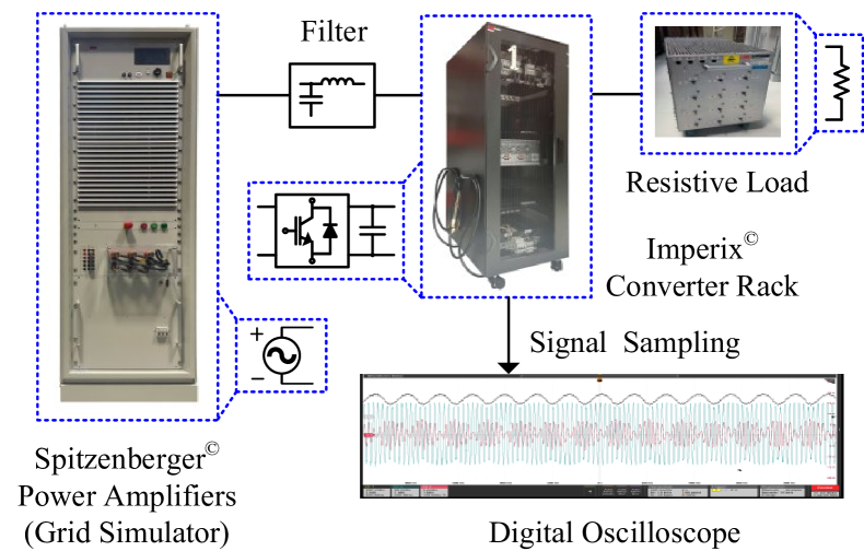
Considering a single-phase converter of electric trains as shown in Fig. 1, low-frequency oscillations (LFO) might occur in electrified railways when multiple trains are energized in the same rail depot under low power conditions [12]. When LFOs occur, there are periodic oscillations of AC-side voltage and current, and DC-side voltage with a frequency of 1 to 10 Hz [12]. The transient direct current control strategy [13] is used in the controller, but the measured signals are independent of the controller due to the assumption of black-box conditions with an unknown controller structure. To assess system stability with data-driven methods, the dataset of system states is collected from an experimental platform of the downscaled single-phase converter as shown in Fig. 2, and Table I lists the main system parameters.
| Parameter | Description | Value |
|---|---|---|
| Grid phase voltage (RMS) | 110 V | |
| Grid-side inductance | 8 mH | |
| Converter-side inductance | 4 mH | |
| Filter capacitance | 10 uF | |
| DC link voltage of the converter | 170 V | |
| DC link Load resistance | 460 | |
| DC link support capacitance | 800 uF | |
| Switching frequency | 10 kHz |
II-B DMD Algorithm
Based on the spatio-temporal snapshots of discrete measurement data, DMD can find a best-fit solution of the dynamic matrix for oscillation mode identification as shown in Fig. 3, where dynamic matrix is the mapping relationship between a pair of data matrices with time shift, governing the inherent dynamic evolution of a discrete linear system [8]. In Fig. 3, denotes an element of the measurable discrete system states, where is the index of system states, is the total number of system states, is the index of temporal iterations, and is the total number of temporal iterations with regular sampling time interval .
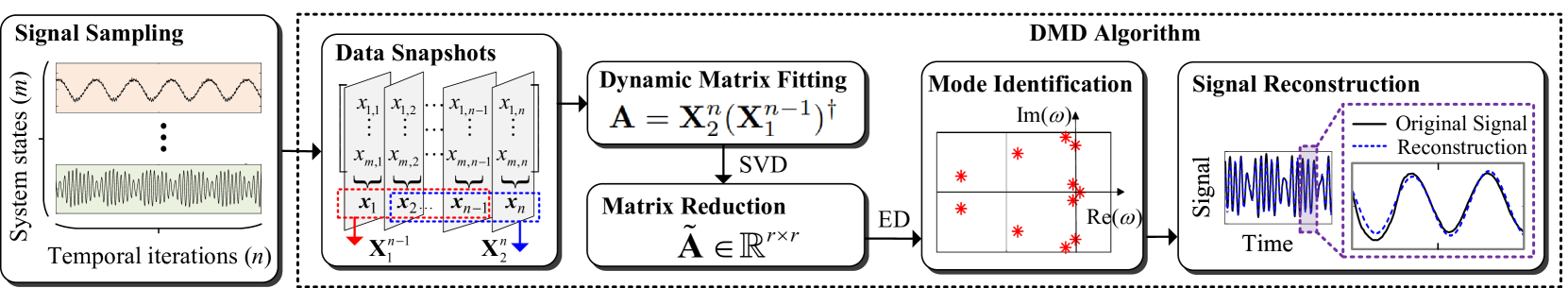
The standard DMD procedure [10] is summarized in Algorithm 1, which starts with generating a pair of data matrices, i.e., and with a time shift, and ends up with the signal reconstruction . It is worth mentioning that, since high order data matrices are required in the DMD algorithm but there are limited measurable channels in power converter systems, the data-stacking technique [14] needs to be used before executing the algorithm to increase the row number () of the data matrix and ensure all significant modes are contained.
In the DMD algorithm, the dynamic matrix is obtained in step 1, where denotes the Moore-Penrose pseudo-inverse. Then, singular value decomposition (SVD) with the truncation rank is implemented to calculate the pseudo-inverse of , and a reduced-order matrix with rank can be obtained by projecting the initial full dynamic matrix into an basis subspace. Then, the eigen-decomposition (ED) of is calculated to extract diagonal matrix consisting of eigenvalues, while matrix of DMD exact modes is obtained based on eigenvectors . Finally, the measured signal (data matrix) can be reconstructed, where is defined as the mode amplitude, is the column of matrix , is the mode amplitude with .
However, DMD just deals with all data within the sampling window at once to provide a full-rank approximation of the dynamics observed. As an SVD-based algorithm, a single DMD application can only yield one pair of eigenvalues for the same mode, resulting in poor robustness to correctly capture transient time behaviors within the dataset, which can be observed clearly by the comparison shown in Fig. 4.
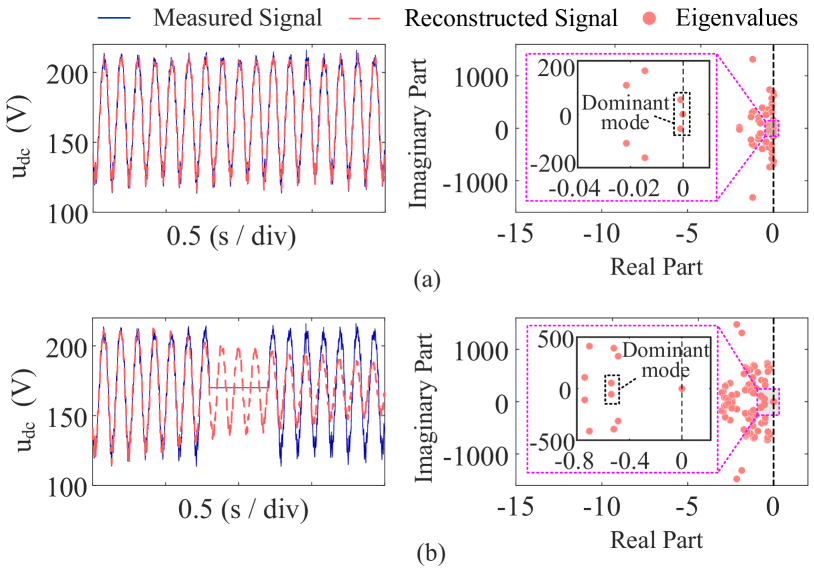
As shown in Fig. 4(a), DMD is capable of reconstructing measured signals and identifying dominant eigenvalues with critical damping, where DC-side voltage is employed as the measured signal to obtain the dataset when the LFO at 8.6 Hz occurs in the experimental platform as shown in Fig. 2. However, it can be seen from Fig. 4(b) that, if there is transient time behavior in the signal such as missing data, DMD will fail to perform well. To be specific, there is a large error in the damping of dominant eigenvalues, showing incorrect stability assessment results. Moreover, the measured signal cannot be reconstructed accurately.
III Mode Identification with MR-DMD
III-A MR-DMD Algorithm
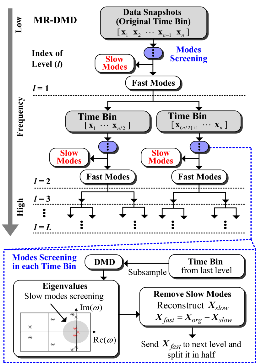
By integrating the conventional DMD algorithm with multi-resolution analysis from wavelet theory [15], multi-resolution dynamic mode decomposition (MR-DMD) applies DMD recursively in different spatio-temporal subsamples [11]. In the MR-DMD algorithm, oscillation modes with relatively low frequency and slow growth/decay rate are defined as slow modes, so their corresponding eigenvalues are close to the origin of the complex plane. As shown in Fig. 5, slow modes can be screened after performing the DMD algorithm on the available dataset (i.e., original time bin), and then the DMD approximation is found from only the slow modes. After that, the slow-mode approximation is removed from the available dataset, and the remaining part representing fast modes is split in half to obtain two equal time bins. The above steps are repeated recursively for each time bin in different decomposition levels until a desired truncation level is achieved. It is worth noting that, since only the slow modes at each decomposition level are captured, it is important to subsample with a fixed small number in each time bin, which can not only improve the computational efficiency but also ensure the maximum frequency of capturable mode increase with increasing decomposition level.
III-B Parameter Derivation
According to the steps of MR-DMD as shown in Fig. 5, three important parameters affecting algorithm performance need to be clearly defined, i.e., the fixed subsample number of each time bin (), the termination level (), and the screening threshold of slow modes ().
The recursion process of MR-DMD shows that, if the index of decomposition levels is defined as , the number of time bins in different levels can be expressed as , so the size of each time bin in different levels will be , where has been defined as the total number of initial sampling points. Since the state signal is sampled with a regular time interval , there is , where is the sampling window duration of the original dataset. Therefore, the time window duration of each time bin () is derived as:
| (1) |
Subsampling with a fixed number is indispensable before implementing DMD in each time bin, so the subsample frequency is obtained by calculating the reciprocal of the subsampling interval as:
| (2) |
Based on the Nyquist sampling theorem, the maximum frequency of capturable modes is obtained as:
| (3) |
Since has been determined after obtaining the original dataset, it can be seen from (3) that, depends on and , which explains why the maximum frequency of capturable mode increase with increasing decomposition level after performing subsampling. Moreover, can be determined based on required for each decomposition level.
The size of time bins in the highest level should be larger than the subsample number of each time bin, otherwise subsampling will fail to perform. Therefore, the selection criterion for the termination level is expressed as:
| (4) |
Hence, is affected by . To be specific, has to be decreased if increases to some extent.
Regarding screening of slow modes, When a discrete eigenvalue identified by MR-DMD enable to hold, the corresponding mode can be regarded as slow mode, but screening threshold of slow modes is still not defined clearly. To this end, we assume the relationship between and the maximum frequency of slow modes in each decomposition level is , which can be further written as:
| (5) |
Where, is an arbitrary constant rational number larger than 1, and represents continuous eigenvalue in the complex plane.
The relationship between the discrete eigenvalue and continuous eigenvalue is [10], which can be rewritten after subsampling as:
| (6) |
The key eigenvalues corresponding to slow modes are usually located near the imaginary axis, indicating their real parts are much smaller than imaginary parts, so is assumed to be valid. As a result, is obtained by combining (5) and (6), thereby can be regarded as the screening threshold of slow modes .
IV Experimental Results
IV-A Data Sampling and Processing
Based on the experimental platform as shown in Fig. 2, the dataset is collected in a sampling window of 2 seconds with a frequency of 2500 Hz, respectively using DC-side voltage and AC-side current as the measured signal in two cases. Hence, the total number of sampling points is 5000. Data stacking technique is employed to preprocess the data and stacking number is set as 1000, ending up with a data matrix of 1000 rows by 4000 columns , so the sampling window duration is considered as 1.6 seconds. To verify robustness, the dataset was set up with missing data.
IV-B Parameter Setting and Results
IV-B1 DC-side voltage as measured signal
The frequency of oscillation component in denoted as is usually lower than 10 Hz. According to (3) and related discussion, it can be found that a smaller leads to more decomposition levels in the low-frequency range, allowing for finer identification of LFO. Therefore, subsample number of each time bin is set as 16, indicating that the maximum frequency of capturable modes in each level is expected to be Hz , where the termination level can be calculated as 8 based on (4). The screening threshold of slow modes is set as , meaning that modes with frequencies less than in each level are regarded as slow modes. Hence, the maximum frequency of slow modes in each level should be Hz.
As shown in Fig. 6(a), by superimposing all 8 decomposition levels, the final reconstructed signal aligns closely with the original measured signal showing oscillations at approximately 8.6 Hz. It can also be found that Level 1 determines the basis of the signal (DC component), while Level 4 serves a significant role in identifying the low-frequency oscillation, and higher levels provide further fine fitting of the higher harmonics. All identified eigenvalues and eigenvalues of slow modes in each decomposition level are shown in Fig. 6(b), where increases from 5 Hz in Level 1 to 640 Hz in Level 8. Since the screening threshold is set as , slow modes marked by red points are screened in the frequency range from less than 1.25 Hz in Level 1 to less than 160 Hz in Level 8, which is consistent with the designed through parameter setting.
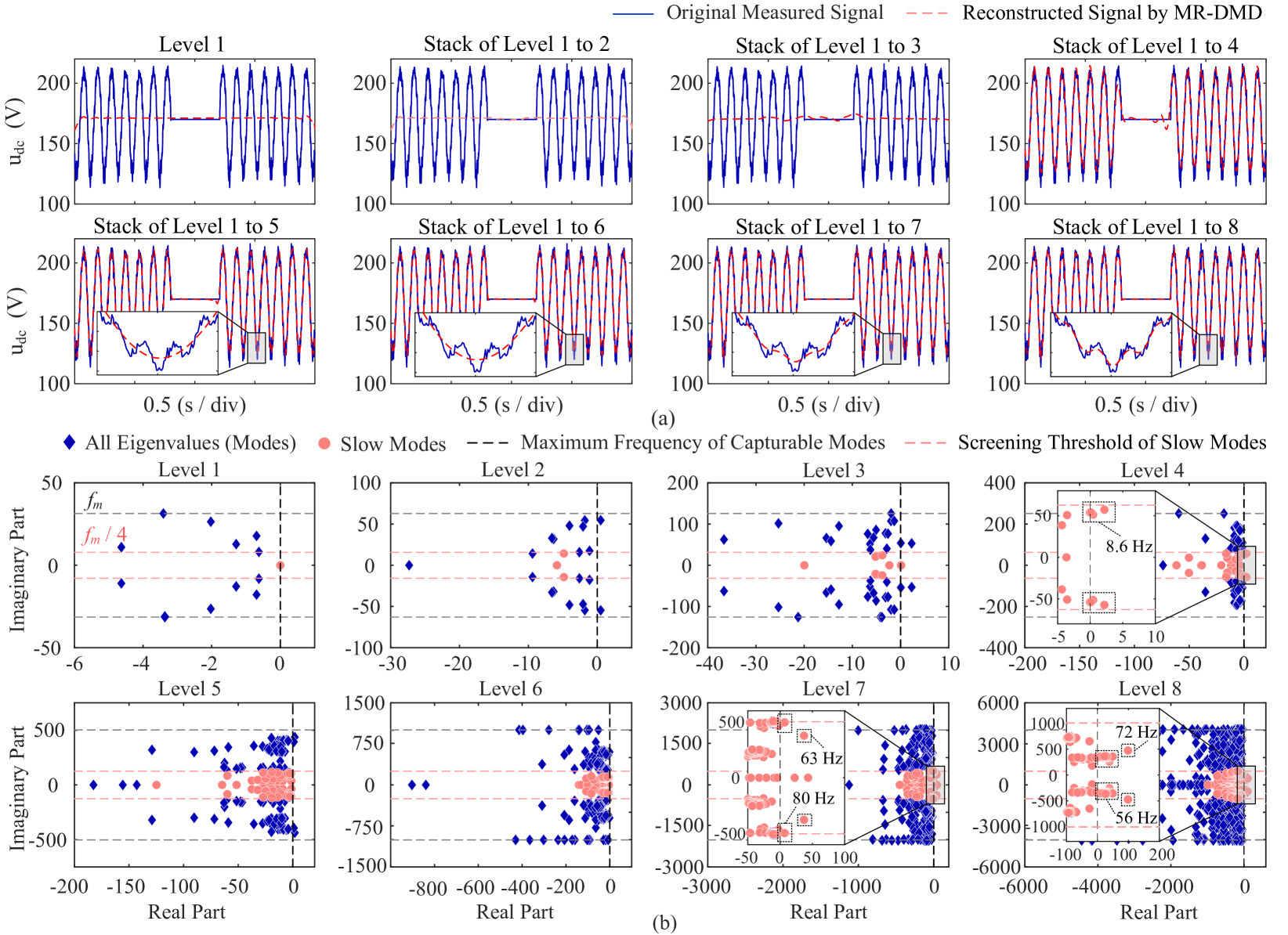
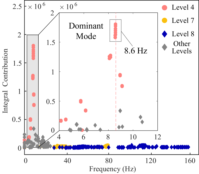
In addition, eigenvalues (modes) with critical or negative damping are shown in Level 4, 7, and 8, but the integral contribution representing the importance of each eigenvalue [16] shown in Fig. 7 indicates that the mode with a frequency of 8.6 Hz in Level 4 is the dominant mode, matching the results in Fig. 6(a). More importantly, the above results prove that MR-DMD is more robust and can correctly handle the dataset with missing data due to its ability of multi-resolution analysis, which cannot be achieved by conventional DMD.
IV-B2 AC-side current as measured signal
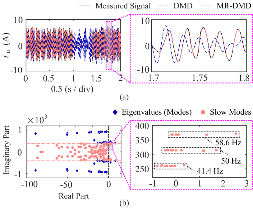
When LFO occurs, the frequency transformation of ac-dc converters translates the oscillation component at the dc-side into two components of the frequencies at the ac-side, where is the grid fundamental frequency (50 Hz). Thus, can be set as 50 in this case, and the corresponding in each level is calculated as Hz , where will be 6. Finally, in each level should be Hz, when is also set as .
As shown in Fig. 8(a), conventional DMD fails to reconstruct measured siganl, but the final reconstructed signal of MR-DMD by superimposing all 6 decomposition levels aligns closely with the measured signal, and the envelope of the waveform shows an oscillation at 8.6 Hz. The reconstructed signals in each level will not be shown for brevity, but it is worth mentioning that the reconstruction of AC waveforms near the fundamental frequency is realized in Level 5, which is consistent with the calculation result of .
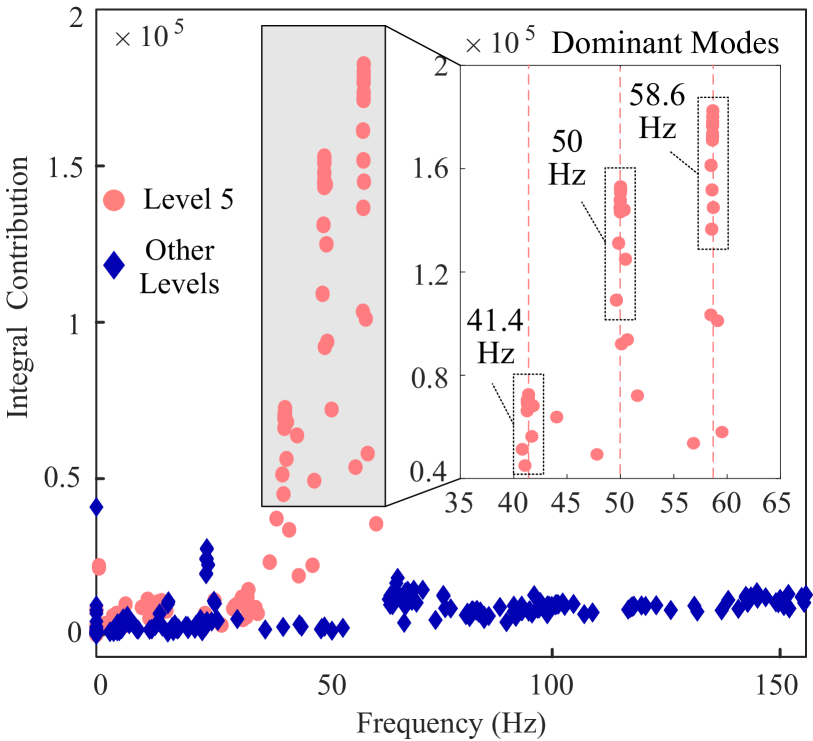
Moreover, identified eigenvalues in Level 5 by MR-DMD are shown in Fig. 8(b). In addition to the fundamental frequency component at 50 Hz, there are two groups of dominant modes with critical or negative damping at 41.4 Hz and 58.6 Hz respectively, matching the results of integral contribution as shown in Fig. 9. The above analysis can also accurately identify the occurrence of LFO at 8.6 Hz in the system.
V Conclusion
In this paper, a diagnostic and identification tool for system stability of power electronic converters is proposed based on multi-resolution dynamic mode decomposition (MR-DMD), which hierarchically decomposes datasets into multiple time bins and applies conventional DMD recursively, where slow modes in different decomposition levels and time scales are screened. Three crucial parameters of MR-DMD are derived to reveal the frequency range of eigenvalues captured in each decomposition level and the screening threshold for slow modes. The identification results indicate that, compared with the conventional DMD algorithm, MR-DMD can accurately identify dominant oscillation modes and reconstruct measured signals using a dataset with transient time behavior. To extend the scope of this article in the future, the influence mechanism and design framework of algorithm parameters can be further analyzed to achieve optimal identification.
References
- [1] X. Wang and F. Blaabjerg, “Harmonic stability in power electronic-based power systems: Concept, modeling, and analysis,” IEEE Trans. Smart Grid., vol. 10, no. 3, pp. 2858–2870, 2019.
- [2] N. Pogaku, M. Prodanovic, and T. C. Green, “Modeling, analysis and testing of autonomous operation of an inverter-based microgrid,” IEEE Trans. Power Electron., vol. 22, no. 2, pp. 613–625, 2007.
- [3] M. Cespedes and J. Sun, “Impedance modeling and analysis of grid-connected voltage-source converters,” IEEE Trans. Power Electron., vol. 29, no. 3, pp. 1254–1261, 2014.
- [4] L. Fan, “Data fusion-based distributed prony analysis,” Electric Power Syst. Res., vol. 143, pp. 634–642, 2017.
- [5] H. Ye, Y. Song, Z. Zhang, and C. Wen, “Global dynamic event-triggered control for nonlinear systems with sensor and actuator faults: A matrix pencil based approach,” IEEE Trans. Automat Contr., pp. 1–8, 2023.
- [6] G. E. Mejia-Ruiz, R. Cárdenas-Javier, M. R. Arrieta Paternina, J. R. Rodríguez-Rodríguez, J. M. Ramirez, and A. Zamora-Mendez, “Coordinated optimal volt/var control for distribution networks via d-pmus and ev chargers by exploiting the eigensystem realization,” IEEE Trans. Smart Grid., vol. 12, no. 3, pp. 2425–2438, 2021.
- [7] A. Almunif, L. Fan, and Z. Miao, “A tutorial on data-driven eigenvalue identification: Prony analysis, matrix pencil, and eigensystem realization algorithm,” Int. Trans. Elect. Energy Syst., vol. 30, no. 4, 2020.
- [8] P. J. Schmid, “Dynamic mode decomposition of numerical and experimental data,” J. Comput. Dyn., vol. 656, pp. 5–28, 2010.
- [9] V. Klema and A. Laub, “The singular value decomposition: Its computation and some applications,” IEEE Transactions on Automatic Control, vol. 25, no. 2, pp. 164–176, 1980.
- [10] A. Alassaf and L. Fan, “Randomized dynamic mode decomposition for oscillation modal analysis,” IEEE Trans. Power Syst., vol. 36, no. 2, pp. 1399–1408, 2021.
- [11] J. N. Kutz, X. Fu, and S. L. Brunton, “Multiresolution dynamic mode decomposition,” SIAM J. Appl. Dyn. Syst., vol. 15, no. 2, pp. 713 – 735, 2016.
- [12] H. Hu, Y. Zhou, X. Li, and K. Lei, “Low-frequency oscillation in electric railway depot: A comprehensive review,” IEEE Trans. Power Electron., vol. 36, no. 1, pp. 295–314, 2021.
- [13] R. Kong, S. Sahoo, F. Blaabjerg, X. Lyu, and X. Wang, “Controller stability and low-frequency interaction analysis of railway train-network systems,” European Conf. Power Electron. Appl., EPE ECCE Europe, pp. 1–9, 2023.
- [14] E. V. Filho and P. Lopes dos Santos, “A dynamic mode decomposition approach with hankel blocks to forecast multi-channel temporal series,” IEEE Control Syst Lett., vol. 3, no. 3, pp. 739–744, 2019.
- [15] T. Guo, T. Zhang, E. Lim, M. López-Benítez, F. Ma, and L. Yu, “A review of wavelet analysis and its applications: Challenges and opportunities,” IEEE Access., vol. 10, pp. 58 869–58 903, 2022.
- [16] G. N. Baltas, N. B. Lai, C. Sabillon, J. Cao, and P. Rodriguez, “Impedance mapping in smart grids with dynamic mode decomposition,” IEEE Energy Convers. Congr. Expo., ECCE, pp. 1–6, 2022.