A note on heterogeneity, trade integration and spatial inequality

Abstract

We study the impact of economic integration on spatial development in a model where all consumers are inter-regionally mobile and have heterogeneous preferences regarding their residential location choices. This heterogeneity is the unique dispersion force in the model. We show that, under reasonable values for the elasticity of substitution among varieties of consumption goods, a higher trade integration always promotes more symmetric patterns, irrespective of the functional form of the dispersion force. We also show that an increase in the degree of heterogeneity in preferences for location leads to less spatial inequality.

Keywords: heterogeneous location preferences; economic integration; economic geography; spatial development.

JEL codes: R10, R12, R23

1 Introduction

In this paper, we study the possible spatial distributions in the $2$-region Core-Periphery (CP) model by Murata (2003), where all labour is free to migrate between regions and workers are heterogeneous regarding their preferences for location. Our aim is to investigate how spatial patterns evolve as regions become more integrated and whether the degree of heterogeneity has qualitative impact on this relationship. Heterogeneity in preferences for location generates a local dispersion force (akin to congestion), which we model as a utility penalty, following the recent work of Castro et al. (2022). This framework can been shown to encompass various functional forms used in discrete choice models of probabilistic migration, including the well-known Logit model (used e.g. by Murata, 2003; Tabuchi and Thisse, 2002).

We show that, irrespective of the degree of heterogeneity, a higher trade integration always promotes more symmetric spatial patterns. Since heterogeneity does not co-vary with transportation costs, the latter only affect the strength of agglomeration forces due to increasing returns. This is a reversion of the usual prediction that lower transport costs lead to agglomeration, and contrasts the findings that consumer heterogeneity leads to a bell-shaped relationship between decreasing transport costs and spatial inequality (Murata, 2003; Tabuchi and Thisse, 2002). Since there is no immobile workforce (no fixed regional internal demand), there is a lower incentive for firms to relocate to smaller markets in order to capture a higher share of local demand and avoid competition when transport costs are higher. Krugman and Elizondo (1996), Helpman (1998) and Murata and Thisse (2005), have also obtained similar results concerning the relationship between transportation costs and spatial inequality. The first includes a congestion cost in the core, the second considers a non-tradable housing sector and the treatment is only numerical, while the latter’s prediction cannot be disassociated from the interplay between inter-regional transportation costs and intra-regional commuting costs. Recently, Tabuchi et al. (2018) have reached similar conclusions to ours arguing that falling transport costs increase the incentives for firms in peripheral regions to increase production since they have a better access to the core, thus contributing to the dispersion of economic activities. Allen and Arkolakis (2014) estimated that the removal of the US Interstate Highway System, which, by limiting accesses, can be interpreted as an increase in transportation costs, would cause a redistribution of the population from more economically remote regions to less remote regions in the US. This adds empirical validity to our findings.

The rest of the paper is organized as follows. In section 2 we describe the model and the short-run equilibrium. In section 3 we study the qualitative properties of the long-run equilibria. Finally, section 4 is left for some concluding remarks.

2 The model

There are two regions $L$ and $R$ with a total population of mass $1$. Consumers are assumed to have heterogeneous preferences with respect to the region in which they reside. We follow Castro et al. (2020) and assume that these preferences are described by a parameter $x,$ uniformly distributed along the interval $[0,1]$. The consumer with preference described by $x=0$ (resp. $x=1$) has the highest preference for residing in region $L$ (resp. region $R$). An agent whose preference corresponds to $x=1/2$ is indifferent between either region. We can thus refer to each consumer with respect to his preference towards living in region $L$ as $x\in[0,1]$.

For a consumer with preference $x$, the utilities from living in region $L$ and $R$ are given, respectively, by:

$$U_{L}(x)= U\left(u\left(C_{L}\right),t(x)\right)$$

$$U_{R}(x)= U\left(u\left(C_{R}\right),t(1-x)\right),$$ (1)

where $C_{i}$ denotes the level of consumption of a consumer living in region $i\in\left\{L,R\right\}$, and $t(x)$ is the utility penalty associated with living in $L$, while $t(1-x)$ is the utility penalty a consumer faces from living in region $R.$ Regions are symmetric in all respects. We assume that $t^{\prime}(.)>0$. There are two regions $L$ and $R$ with a total population of mass $1$.

The short-run equilibrium is equivalent to Murata (2003) and Tabuchi et al. (2018), which we briefly describe here. The consumption aggregate is a CES composite given by:

$$C=\left[\int_{s\in S}c(s)^{\tfrac{\sigma-1}{\sigma}}ds\right]^{\tfrac{\sigma}{\sigma-1}},$$

where $s$ stands for the variety produced by each monopolistically competitive firm and $\sigma$ is the constant elasticity of substitution between any two varieties. The consumer is subject to the budget constraint $P_{i}C_{i}=w_{i}$, where $P_{i}$ is the price index and $w_{i}$ is the nominal wage in region $i$. Utility maximization by a consumer in region $i$ yields the following demand for each manufactured variety produced in $j$ and consumed in $i$:

$$c_{ij}=\dfrac{p_{ij}^{-\sigma}}{P_{i}^{1-\sigma}}w_{i},$$ (2)

where:

$$P_{i}=\left[\int_{s\in S}p_{i}(s)^{1-\sigma}d(s)\right]^{\tfrac{1}{1-\sigma}},$$ (3)

is the manufacturing price index for region $i$. A manufacturing firm faces the following cost function:

$$TC(q)=w\left(\beta q+\alpha\right),$$

where $q$ corresponds to a firm’s total production of manufacturing goods, $\beta$ is the input requirement (per unit of output) and $\alpha$ is the fixed input requirement. The manufacturing good is subject to trade barriers in the form of iceberg costs, $\tau\in(1,+\infty)$: a firm ships $\tau$ units of a good to a foreign region for each unit that arrives there. Assuming free entry in the manufacturing sector, at equilibrium firms will earn zero profits, which translates into the following condition:

$$\pi\equiv\left(p-\beta w\right)q-\alpha w =0,$$

which gives the firm’s total equilibrium output, symmetric across regions:

$$q_{L}=q_{R}=\frac{\alpha(\sigma-1)}{\beta},$$ (4)

and the following profit maximizing prices:

$$p_{LL}=\dfrac{\beta\sigma}{\sigma-1}w_{L}\text{ \ and\ }p_{RL}=\dfrac{\beta\sigma\tau}{\sigma-1}w_{L}.$$ (5)

Labour-market clearing implies that the number of agents in region $L$ equals labour employed by a firm times the number of varieties produced in a region:

$$h=n_{L}\left(\alpha+\beta q_{L}\right),$$

from where, using (4), we get:

$$n_{L}=\dfrac{h}{\sigma\alpha}\text{ \ and \ }n_{R}=\dfrac{1-h}{\sigma\alpha}.$$ (6)

Choosing labour in region $R$ as the numeraire, we can normalize $w_{R}$ to $1$. The price indices in $L$ and $R$ using (3) are given, after (6), by:

$$P_{L} =\left[\dfrac{h}{\sigma\alpha}\left(\dfrac{\beta\sigma}{\sigma-1}w\right)^{1-\sigma}+\dfrac{1-h}{\sigma\alpha}\left(\dfrac{\beta\sigma\tau}{\sigma-1}\right)^{1-\sigma}\right]^{\tfrac{1}{1-\sigma}},$$

$$P_{R} \left[\dfrac{1-h}{\sigma\alpha}\left(\dfrac{\beta\sigma}{\sigma-1}\right)^{1-\sigma}+\dfrac{h}{\sigma\alpha}\left(\dfrac{\beta\sigma\tau}{\sigma-1}w\right)^{1-\sigma}\right]^{\tfrac{1}{1-\sigma}}$$ =. (7)

Rewriting a firm’s profit in region $L$ as:

$$\pi_{L}=\left(p_{LL}-\beta w\right)\left[hc_{LL}+(1-h)\tau c_{RL}\right]-\alpha w,$$

the zero profit condition yields, after using (2), (5) and (7), the following wage equation:

$$h=\dfrac{w^{\sigma}-\phi}{w^{\sigma}-\phi+w(w^{-\sigma}-\phi)},$$ (8)

where $\phi\equiv\tau^{1-\sigma}\in(0,1)$ is the freeness of trade. The nominal wage $w$ can be implicitly defined as a function of the spatial distribution in region $L$, $h\in[0,1]$. We have $w(0)=\phi^{1/\sigma}<1$, $w(1/2)=1$ and $w(1)=\phi^{-1/\sigma}>1$. We say that $L$ is larger than $R$ when $h>1/2,$ and smaller otherwise. Figure 1 illustrates $w(h)$ for $h\in[0,1]$ with parameter values $\sigma=2$ and $\phi=0.5$.

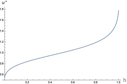
Figure 1: Short-run equilibrium relative wage as a function of the consumers in region $L$. We set $\sigma=2$ and $\phi=0.5$.

The nominal wage is strictly increasing in the spatial distribution (see Appendix A). Moreover, see Appendix A, when $h>1/2$, the relative wage $w$ increases when trade barriers are higher. Conversely, if $h<1/2$, higher trade barriers implies lower wages in $L$. Therefore higher trade barriers increase the wage divergence between the regions.

The intuition is as follows. When all workers are mobile, they can move to the region that offers them a relatively better access to varieties. This advantage of the larger region becomes higher as transport costs increase because markets become more focused on local demand. This increases expenditures in the larger region relative to the smaller, which in turn pushes the nominal relative wage upwards.

We consider a general isoelastic sub-utility for consumption goods:

$$\begin{cases}u_{i}=\dfrac{C_{i}^{1-\theta}-1}{1-\theta},&\text{ if }\theta\in[0,1)\cup(1,+\infty)\\ u_{i}=\ln C_{i},&\text{ if }\theta=1,\end{cases},$$ (9)

where for $\theta=1$ we take the limit value of the upper expression of $u_{i}$. The parameter $\theta$ is a positive agglomeration externality. It influences how a change in the regional consumption differential, $C_{L}-C_{R}$, impacts the regional utility differential, $u_{L}-u_{R}$, i.e., it influences the strength of the self-reinforcing agglomeration mechanism when one region is more populated than the other. We shall detail further below why this specification is useful.

The utility differential from consumption goods, $\Delta u\equiv u_{L}-u_{R},$ is given by:

$$\Delta u=\begin{cases}\dfrac{\eta}{1-\theta}\left\{w^{1-\theta}\left[(1-h)\phi+hw^{1-\sigma}\right]^{\tfrac{1-\theta}{\sigma-1}}-\left[1-h+h\phi w^{1-\sigma}\right]^{\tfrac{1-\theta}{\sigma-1}}\right\},&\ \text{if }\mbox{$\theta\neq$1}\\ \ln w+\dfrac{1}{\sigma-1}\ln\left[\frac{hw^{1-\sigma}+(1-h)\phi}{h\phi w^{1-\sigma}+(1-h)}\right],&\ \text{if $\theta$=1.}\end{cases}$$ (10)

We adopt the normalizations by Fujita et al. (1999), i.e., $\alpha\sigma=1$ so that the number of consumers in a region equals its number of firms. Moreover, we assume that $(\sigma-1)/(\sigma\beta)=1$ so that the price of each manufactured variety in a region equals its workers’ nominal wage. These imply that $\eta=1$.

Figure 2 depicts $\Delta u$ in (10) for different levels of $\theta$.

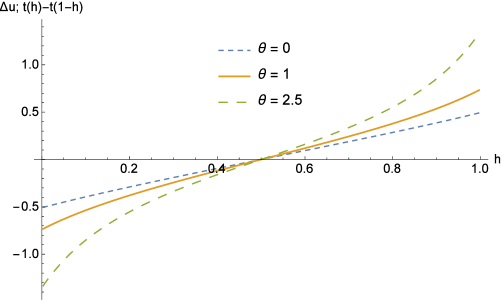
Figure 2: Utility differential $\Delta u=u_{L}-u_{R}$ for different levels of $\theta$. Parameter values are $\sigma=2$ and $\phi=0.5$.

We observe that a higher $\theta$ increases the utility differential $\Delta u$ for any spatial distribution $h>1/2$. Therefore, if $L$ is relatively more industrialized, a higher $\theta$ increases the attractiveness of $L$ relative to $R$ for consumers. Thus, it strengthens the agglomeration forces towards region $L$.

The purpose of the general specification in (9) is explained as follows. Firstly, it allows us to derive general stability conditions for long-run equilibria for any $t(x)$. Secondly, it encompasses the Murata (2003) model as a particular case when $\theta=0$, which is of great interest for comparison purposes.

3 Long-run equilibria

In a long-run spatial equilibrium, each worker chooses to live in the region that provides a higher utility. Hence, as in Castro et al. (2022), a long-run equilibrium must be such that workers with $x\in[0,h)$ live in region $L$ and workers with $x\in(h,1]$ live in region $R$. Knowing from utility maximization that $C=W/P$ and assuming that $t(x)$ enters additively in overall utility $U_{i}(x)$, we rewrite the indirect utilities as:

$$V_{L}(h) =\dfrac{C_{L}^{1-\theta}-1}{1-\theta}-t(h)$$

$$V_{R}(h) =\dfrac{C_{R}^{1-\theta}-1}{1-\theta}-t(1-h),$$ (11)

where $h$ satisfies the short-run equilibrium in (8).

3.1 Interior equilibria

Due to symmetry, we focus only on the case where $L$ is larger or the same size as $R$, i.e., $h\geq 1/2$. We define an interior equilibrium $h^{*}\in[1/2,1)$ as a spatial distribution $h$ that satisfies both (8) and $V_{L}=V_{R}$. Such an equilibrium is said to be stable if $d\left(V_{L}-V_{R}\right)/dh<0$. This leads to the following Lemma.

Lemma 1.

An interior equilibrium $h^{*}\in[1/2,1)$ is stable if:

$$\zeta\left\{\varphi\left[\dfrac{w^{\sigma}+w^{1-\sigma}-(w+1)\phi}{w\left(1-\phi^{2}\right)}\right]^{\frac{\theta-1}{\sigma-1}}-\psi\left[\dfrac{w^{2\sigma}-(w+1)\phi w^{\sigma}+w}{w\left(1-\phi^{2}\right)}\right]^{\frac{\theta+\sigma-2}{\sigma-1}}\right\}<t^{\prime}\left(h^{*}\right)+t^{\prime}\left(1-h^{*}\right),$$

where $h^{*}$ satisfies the short-run equilibrium condition in (8), and:

$$\zeta =\dfrac{w^{-(\theta+\sigma+1)}}{(\sigma-1)\left[(\sigma-1)\phi+(\sigma-1)\phi w^{2\sigma}+\left(-2\sigma+\phi^{2}+1\right)w^{\sigma}\right]};$$

$$\varphi =w\left\{\phi\left[\sigma+(\sigma-1)w\right]w^{\sigma}-2\sigma w+w\right\}\left[w^{2\sigma}-(w+1)\phi w^{\sigma}+w\right];$$

$$\psi =\left(1-\phi^{2}\right)w^{\theta+\sigma+1}\left[(2\sigma-1)w^{\sigma}-\sigma(w+1)\phi+\phi\right].$$

Proof.

See Appendix B. ∎

An interior equilibrium is called symmetric dispersion if $h^{*}=1/2$ and partial agglomeration otherwise. While the former always exists, the latter depends on the form of $t(x)$. Knowing that $w=1$ for $h=1/2$ the stability condition in Lemma 1 for symmetric dispersion simplifies to:

$$\dfrac{d\Delta u}{dh}\left(\tfrac{1}{2}\right)\equiv\frac{2(2\sigma-1)(1-\phi)\left(\frac{1+\phi}{2}\right)^{\frac{1-\theta}{\sigma-1}}}{(\sigma-1)(2\sigma+\phi-1)}<t^{\prime}\left(\tfrac{1}{2}\right).$$ (12)

A careful inspection of (12) allows us to conclude that the LHS is decreasing in $\phi$ if $\theta\geq 1$. For $\theta<1$, it is decreasing in $\phi$ if $\sigma\geq 1+\sqrt{2}/2\approx 1.71$. Symmetric dispersion then becomes easier to sustain under lower transportation costs if $\sigma>1+\sqrt{2}/2$, which, according to recent empirical estimations for $\sigma$, is more than reasonable. Since $t(h)$ does not depend on $\phi$, this result does not depend on consumer heterogeneity. Since, at symmetric dispersion, consumers in each region have access to the same amount of manufactures, an exogenous migration will induce a lower (higher) benefit from local consumption goods in the larger market if transport costs are lower (higher). This is captured by the fact that the relative decrease in prices and increase in wages (at the symmetric equilibrium) is more pronounced when transport costs are higher.

Let us now assume that a partial agglomeration $h^{*}\in(1/2,1)$ equilibrium exists and is unique. Regarding the influence of trade integration on partial agglomeration equilibria, we establish the following result.

Proposition 1.

If a stable partial agglomeration $h^{*}\in(1/2,1)$ exists and is unique, it becomes more symmetric as trade barriers decrease.

Proof.

See Appendix C. ∎

This proposition states that if most consumers reside in region $L$, increasing the freeness of trade will lead to a smooth exodus from region $L$ to region $R$, irrespective of the value of $t(h^{*})$. More integration thus increases the incentives for consumers to distribute more equally among the two regions.

3.2 Logit preferences

For the two region case, and following Tabuchi and Thisse (2002) and Murata (2003), the probability that a consumer will choose to reside in region $L$ is given by the logit model written as:

$$P_{L}(h)=\dfrac{e^{u_{L}(h)/\mu}}{e^{u_{L}(h)/\mu}+e^{u_{R}(h)/\mu}},$$ (13)

where $\mu\geq 0$ is a scale parameter which measures the dispersion of consumer preferences. If $\mu=0$, consumers do not care about their location preferences but rather solely about relative wages. The number of agents $h$ is the same as the consumer $x$ who is indifferent between living in region $L$ or in region $R$. Therefore, the probability $P_{L}(h)$ is tantamount to the indifferent consumer $x=h$ (Castro et al. 2022). Thus, using (13), we can write:

$$h=\dfrac{e^{u_{L}(h)/\mu}}{e^{u_{L}(h)/\mu}+e^{u_{R}(h)/\mu}}.$$ (14)

Manipulating (14) yields:

$$u_{L}-\mu\ln h=u_{R}-\mu\ln(1-h),$$ (15)

which rearranged yields the long-run equilibrium condition, $\Delta u(h)=\Delta t(h),$ where $\Delta t(h)=\mu\left[\ln h-\ln(1-h)\right]$.

Notice from the (15) that $t(h)=\mu\ln h<0$ for $h\in[0,1]$, so that the overall utility here is interpreted as the utility from consumption plus a benefit from living in the most preferred region. The overall utility of a consumer in region $i$ thus lies on the interval $[U_{i},+\infty)$. For a strictly positive $\mu$, the consumer who likes region $R$ the most (at $x=1$) will never want to live in $L$, because, at $h=1$, the overall utility gain from moving from region $L$ to region $R$ is infinite. This means that the Logit model penalizes (benefits) the consumers who are less (more) willing to leave a region very strongly. Therefore, agglomeration in any region is not possible.

This discussion allows us to formalize the following result, which summarizes the possible spatial outcomes under Logit type preferences, depending on the degree of heterogeneity $\mu.$

Proposition 2.

Under Logit type preferences, the spatial distribution depends on the level of consumer heterogeneity as follows:

• Symmetric dispersion is the only stable equilibrium if:

  $$\mu>\mu_{d}\equiv\dfrac{(2\sigma-1)(1-\phi)}{(\sigma-1)(2\sigma+\phi-1)};$$ (16)

• Partial agglomeration $h^{*}\in\left(\tfrac{1}{2},1\right)$ is the only stable equilibrium if $\mu<\mu_{d}$.

Proof.

See Appendix E. ∎

When consumer heterogeneity is low there is a single stable partial agglomeration equilibrium that is very asymmetric (close to agglomeration). As consumer heterogeneity increases, partial agglomeration corresponds to a more even distribution. Finally, if consumer heterogeneity is high enough ($\mu>\mu_{d}$ in (16)), consumers disperse symmetrically across the two regions.

In Figure 3 we show how the spatial distribution of industry changes as regions become more integrated. We set $\sigma=2.5$ and $\mu=0.2$.

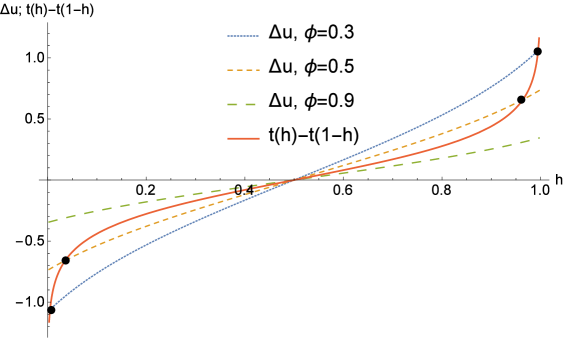
Figure 3: Utility differential $\Delta u$ (dashed lines) and penalty differential $t(h)-t(1-h)$ (thick line) for increasing levels of $\phi$. For $\phi=0.3$ (upper dashed line), dispersion is unstable and partial agglomeration is stable. For$\phi=0.5$ (medium dashed line) dispersion is unstable, partial agglomeration is stable and is less asymmetric. For $\phi=0.9$ (lower dashed line) dispersion is stable and is the only equilibrium. The values for the parameters are $\sigma=2.5$ and $\mu=0.2$.

For low levels of the freeness of trade, a unique stable partial agglomeration equilibrium exists where most consumers reside in region $L$. This means that there is just a small fraction of consumers in $R$ that are not willing to forego their preferred region because the gain in consumption goods from doing so is not high enough. As regions become more integrated, the home-market effect becomes weaker and partial agglomeration becomes more symmetric. Finally, for a high level of inter-regional integration, agglomeration forces are so weak that no consumer is willing to leave his most preferred region and only symmetric dispersion is stable.

The preceding analysis is summarized in the two bifurcation diagrams in Figure 4, along a smooth parameter path where $\mu$ and $\phi$ increase. We numerically uncover two supercritical pitchfork bifurcations in $\mu$ and $\phi$. The picture to the right in Figure 4 (increasing $\phi$) differs from other supercritical pitchforks found in the literature (e.g., Pflüger, 2004; Ikeda et al., 2022) crucially in the sense that the direction of change in stability as $\phi$ increases is reversed, i.e., lower trade barriers leads to more symmetric spatial distributions.

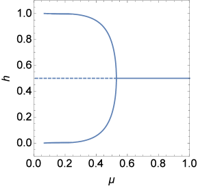
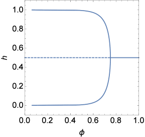
Figure 4: Bifurcation diagrams. To the left, the bifurcation parameter is $\mu\in[0,1]$ with $\phi=0.4$. To the right, we have $\phi\in(0,1)$ as the bifurcation parameter and set $\mu=0.2$. For both scenarios we use $\sigma=2$.

4 Discussion and concluding remarks

We have seen that heterogeneity in preferences for location alone bears no impact on the relationship between trade integration and spatial inequality, which is a monotonic decreasing one. This contrasts the findings in other works with heterogeneity in consumer preferences, such as Tabuchi and Thisse (2002) and Murata (2003), who show evidence of a bell-shaped relationship between trade integration and spatial inequality. The former’s setting differs from ours because the authors consider an inter-regionally immobile workforce whose role as a dispersive force is enhanced by higher transportation costs.

However, it is particularly worthwhile to discuss the results of Murata (2003). Murata (2003) found that the relationship between trade integration and spatial inequality need not be monotonic and depends on the degree of consumer heterogeneity, which is at odds with our findings. For instance, for an intermediate degree of consumer heterogeneity, Murata finds that increasing trade integration initially fosters agglomeration and later leads to re-dispersion of industry. However, these conclusions can be shown to stem from the author’s particular choice of the value for the elasticity of substitution, $\sigma=1.25$. As we have argued in Section 3, such a low value is empirically implausible. For exceedingly low values $(\sigma<1.71)$, increasing returns at the firm level are too strong. Strong enough that the utility gain at dispersion becomes increasing in $\phi$, instead of decreasing. This would justify an initial concentration of industry as a result of an increase in $\phi.$ However, we have seen that for a plausible range of $\sigma$ the utility gain at dispersion always decreases with $\phi$. Moreover, if $\theta>0$, this holds even for lower values of $\sigma$. Therefore, a higher $\phi$ always promotes more equitable distributions as opposed to asymmetric ones.

Hence, when workers are completely mobile, more trade integration ubiquitously reduces the spatial inequalities between the two regions, irrespective of the degree of heterogeneity in location preferences. Therefore, a de facto lower inter-regional labour mobility induced by consumer heterogeneity alone cannot account for the predictions that a higher inter-regional integration will lead to more unequal spatial development or an otherwise bell-shaped relationship between the two.

By considering that all consumers are allowed to migrate if they so desire, we have shown that a higher inter-regional trade integration always leads to less spatial inequality. This result is independent of the level and impact of consumer heterogeneity. This conclusion may be of potential use for policy makers. Namely, the predictions that globalization is likely to lead to more spatial inequality (World Bank, 2009) in the future may be reversed if policies are undertaken to promote inter-regional mobility.

Appendix A - Wages and freeness of trade

Consider $h=f(w)$ in (8). Let us now define $F(h,w)=f(w)-h=0.$ Differentiation of $F(h,w)$ yields:

$$\dfrac{\partial F(h,w)}{\partial w}=\dfrac{w^{\sigma}G(w^{\sigma})}{\left[w^{2\sigma}-(w+1)\phi w^{\sigma}+w\right]^{2}},$$ (17)

where:

$$G(w^{\sigma})=-\left[\phi(\sigma-1)+(\sigma-1)\phi w^{2\sigma}-\left(2\sigma-\phi^{2}-1\right)w^{\sigma}\right].$$

The derivative in (17) is zero if $G(w^{\sigma})=0$. One can observe that $G(w^{\sigma})$ has either two (real) zeros given by some $\left\{w^{-},w^{+}\right\},$ or none. Moreover, $G(w^{\sigma})$ is concave in $w^{\sigma}.$ Since $G\left(w^{\sigma}=\phi\right)=\sigma\left[\phi(1-\phi^{2})\right]>0$ and $G\left(w^{\sigma}=\phi^{-1}\right)=-\left[\sigma\phi\left(1-\phi^{-2}\right)\right]>0$, it must be that $G(w^{\sigma})>0$ for $w^{\sigma}\in[\phi,\phi^{-1}]\subset(w^{-},w^{+})$.

We now proceed to show that $w\in\left(0,\phi^{1/\sigma}\right)$ and $w\in\left(\phi^{-1/\sigma},+\infty\right)$ are not defined in $h\in[0,1]$. Using (9), we have the following:

$$\lim_{w\rightarrow 0}h(w)=0;\quad\lim_{w\rightarrow+\infty}h(w)=1;\quad h(\phi^{1/\sigma})=0;\quad h(\phi^{-1/\sigma})=1;$$

Since $dh/dw=\partial F/\partial w$, we have that $h(w)$ is increasing for $w^{\sigma}\in(w^{-},w^{+})$. The limits above, together with the knowledge that the zeros of $dh/dw$ lie to the left and right of $[\phi,\phi^{-1}]$, ensure that $h(w)<0$ for $w\in\left(0,\phi^{1/\sigma}\right)$ and $h(w)>1$ for $w\in\left(\phi^{-1/\sigma},+\infty\right)$.

Knowing that $\partial F/\partial h=-1$ and $\partial F/\partial w$ are continuous, by the IFT we can write $w:h\in[0,1]\subset\mathbb{R}\mapsto\mathbb{R}$ such that $dw/dh$ exists and $F(h,w(h))=0$.

Using implicit differentiation on (8), we get:

$$\dfrac{dw}{dh}=\frac{\left[w^{2\sigma}-(w+1)\phi w^{\sigma}+w\right]^{2}}{w^{\sigma}G(w^{\sigma})}.$$ (18)

This derivative is positive for $w\in[\phi^{1/\sigma},\phi^{-1/\sigma}]$, which implies that $w(h)$ is increasing in $[0,1]$.

From $F(h,w)=0$ defined above, differentiating with respect to $\phi,$ we get:

$$\dfrac{\partial F}{\partial\phi}+\dfrac{\partial F}{\partial w}\dfrac{dw}{d\phi} =0\iff$$

$$\dfrac{dw}{d\phi} =-\left.\dfrac{\partial F}{\partial\phi}\right/\dfrac{\partial F}{\partial w}.$$

Using (8) we get:

$$\dfrac{\partial F}{\partial\phi}=\frac{w^{\sigma+1}\left(w^{2\sigma}-1\right)}{\left[w^{2\sigma}-(w+1)\phi w^{\sigma}+w\right]^{2}},$$

which is positive if $h>1/2$, because the latter implies $w>1$ (because $w$ is increasing in $h$). As a result, we have $dw/d\phi<0$. Therefore, the nominal wage $w$ is decreasing in the freeness of trade when $L$ is the largest region ($h>1/2$).

Appendix B - Interior Equilibria

Proof of Lemma 1

Proof.

Taking the derivative of (10) with respect to $h$ yields:

$$\dfrac{d\Delta u}{dh}=-\frac{w^{-(\theta+\sigma)}\left\{w^{\theta}\left(h\phi w^{1-\sigma}-h+1\right)^{-\frac{\theta+\sigma-2}{\sigma-1}}\left[-h(\sigma-1)\phi w^{\prime}-w^{\sigma}+\phi w\right]+\left(hw^{1-\sigma}-h\phi+\phi\right)^{-\left(1+\frac{\theta}{\sigma-1}\right)}\varOmega\right\}}{(\sigma-1)},$$ (19)

where:

$$\Omega=-w\left(hw^{1-\sigma}-h\phi+\phi\right)^{\frac{1}{\sigma-1}}\left[-h(\sigma-1)w^{\prime}-\phi w^{\sigma}+w\right]-(\sigma-1)w^{\sigma}w^{\prime}\left(hw^{1-\sigma}-h\phi+\phi\right)^{\frac{\sigma}{\sigma-1}},$$

Substituting for $w^{\prime}$ using (18) from Appendix A, and given that any partial equilibrium $h^{*}$ must satisfy the short-run equilibrium condition given by (8), we reach:

$$\left.\dfrac{d\Delta u}{dh}\right|_{h=h^{*}}=\zeta\left\{\varphi\left[\dfrac{w^{\sigma-1}+w^{-\sigma}-(1+w^{-1})\phi}{1-\phi^{2}}\right]^{\frac{\theta-1}{\sigma-1}}-\psi\left[\dfrac{w^{2\sigma}-(w+1)\phi w^{\sigma}+w}{w\left(1-\phi^{2}\right)}\right]^{\frac{\theta+\sigma-2}{\sigma-1}}\right\},$$ (20)

with:

$$\zeta =\dfrac{w^{-(\theta+\sigma+1)}}{(\sigma-1)\left[(\sigma-1)\phi+(\sigma-1)\phi w^{2\sigma}+\left(-2\sigma+\phi^{2}+1\right)w^{\sigma}\right]};$$

$$\varphi =w\left\{\phi\left[\sigma+(\sigma-1)w\right]w^{\sigma}-2\sigma w+w\right\}\left[w^{2\sigma}-(w+1)\phi w^{\sigma}+w\right];$$

$$\psi =\left(1-\phi^{2}\right)w^{\theta+\sigma+1}\left[(2\sigma-1)w^{\sigma}-\sigma(w+1)\phi+\phi\right].$$

Since an interior equilibrium is stable if $d\Delta u/dh<d\left[t(h)-t(1-h)\right]/dh$ at $h=h^{*}$, it is stable if (20) is negative, which concludes the proof. ∎

Proof of Proposition 1:

Assume that partial agglomeration $h^{*}=h\in\left(\frac{1}{2},1\right)$ exists and is stable. Then, according to Castro et al. (2020, Prop. 9, pp. 197), it becomes more symmetric if $\frac{d\Delta u}{d\phi}<0$. We have:

$$\dfrac{d\Delta u}{d\phi}=\frac{\partial\Delta u}{\partial\phi}+\frac{\partial\Delta u}{\partial w}\frac{dw}{d\phi},$$

which, by using (8) and (10), becomes:

$$-\frac{w}{a_{3}}\left\{a_{1}\left[-\frac{\left(\phi^{2}-1\right)w^{\sigma+1}}{w^{2\sigma}-(w+1)\phi w^{\sigma}+w}\right]^{-\frac{\theta+\sigma-2}{\sigma-1}}+a_{2}\left[\frac{w-w\phi^{2}}{w^{2\sigma}-(w+1)\phi w^{\sigma}+w}\right]^{-\frac{\theta+\sigma-2}{\sigma-1}}\right\}$$ (21)

where:

$$a_{1} =w^{1-\theta}\left(\phi w^{\sigma}-1\right)\left[-2\sigma+2(\sigma-1)\phi w^{\sigma}+\phi^{2}+1\right]$$

$$a_{2} =w^{-\sigma}\left(w^{\sigma}-\phi\right)\left[2(\sigma-1)\phi+\left(-2\sigma+\phi^{2}+1\right)w^{\sigma}\right]$$

$$a_{3} =(\sigma-1)\left[w^{1-\sigma}+w^{\sigma}-(w+1)\phi\right]\left[(\sigma-1)\phi+(\sigma-1)\phi w^{2\sigma}+\left(-2\sigma+\phi^{2}+1\right)w^{\sigma}\right]$$

Notice that (21) is equivalent to

$$-\frac{w\left[\frac{w-w\phi^{2}}{w^{2\sigma}-(w+1)\phi w^{\sigma}+w}\right]^{-\frac{\theta+\sigma-2}{\sigma-1}}\left(a_{1}w^{-\sigma\frac{\theta+\sigma-2}{\sigma-1}}+a_{2}\right)}{a_{3}}.$$

Thus, the sign of (21) is given by the sign of:

$$-\frac{a_{1}w^{-\sigma\frac{\theta+\sigma-2}{\sigma-1}}+a_{2}}{a_{3}}.$$

Since $w>1$ for $h\in(\frac{1}{2},1]$, we have $a_{3}<0$ because $\left(w^{1-\sigma}+w^{\sigma}-(w+1)\phi\right)>0$ and

$$\left[(\sigma-1)\phi+(\sigma-1)\phi w^{2\sigma}+\left(-2\sigma+\phi^{2}+1\right)w^{\sigma}\right]<0.$$

Next, evaluating the numerator at $\theta=1$, we get:

$$w^{-\sigma}\left(\phi w^{\sigma}-1\right)\left[-2\sigma+2(\sigma-1)\phi w^{\sigma}+\phi^{2}+1\right]+w^{-\sigma}\left(w^{\sigma}-\phi\right)\left[2(\sigma-1)\phi+\left(-2\sigma+\phi^{2}+1\right)w^{\sigma}\right]<0.$$

Differentiating the numerator with respect to $\theta$ yields:

$$\frac{\ln(w)w^{\frac{\theta-1}{\sigma-1}+\sigma}\left(\phi w^{\sigma}-1\right)\left[-2\sigma+2(\sigma-1)\phi w^{\sigma}+\phi^{2}+1\right]}{\sigma-1},$$

which is positive because $1<w^{\sigma}<1/\phi$ and $\left[-2\sigma+2(\sigma-1)\phi w^{\sigma}+\phi^{2}+1\right]<0$. Thus, the numerator of (21) remains negative for all $\theta<1$. We conclude that (21) is negative and thus $\frac{d\Delta u}{d\phi}<0$ for any $\theta\in[0,1]$. This concludes the proof. $\square$

Appendix C - Logit heterogeneity

Proof of Proposition 2:

When $t(x)=\mu\ln x$, the RHS of expression (20) is given by:

$$t^{\prime}\left(h^{*}\right)-t^{\prime}\left(1-h^{*}\right)=\mu\left[\dfrac{1}{h(1-h)}\right].$$

Replacing in (20) and rearranging, partial agglomeration is stable if:

$$-\frac{w^{-\sigma-1}\left[w^{2\sigma}-(w+1)\phi w^{\sigma}+w\right]^{2}\Gamma}{(\sigma-1)\left(w^{\sigma}-\phi\right)\left(1-\phi w^{\sigma}\right)\left[(\sigma-1)\phi+(\sigma-1)\phi w^{2\sigma}+\left(-2\sigma+\phi^{2}+1\right)w^{\sigma}\right]}<0,$$ (22)

where

$$\Gamma =\phi\left[\mu(\sigma-1)^{2}-2\sigma+1\right]+\phi\left[\mu(\sigma-1)^{2}-2\sigma+1\right]w^{2\sigma}-$$

$$-w^{\sigma}\left\{\phi^{2}\left[-(\mu+2)\sigma+\mu+1\right]+(2\sigma-1)\left[\mu(\sigma-1)-1\right]\right\}.$$

The numerator of (22) except $\Gamma$ is positive, and so is $\left(w^{\sigma}-\phi\right)\left(1-\phi w^{\sigma}\right)$. We have:

$$(\sigma-1)\phi+(\sigma-1)\phi w^{2\sigma}+\left(-2\sigma+\phi^{2}+1\right)w^{\sigma}<0.$$

Therefore, (20) holds if and only if $\Gamma<0$, which gives:

$$\mu>\mu_{p}\equiv\frac{(2\sigma-1)(w^{\sigma}-\phi)(1-w^{\sigma}\phi)}{(\sigma-1)\left[\left(2\sigma-\phi^{2}-1\right)w^{\sigma}-(\sigma-1)\phi w^{2\sigma}-(\sigma-1)\phi\right]}.$$

The condition for partial agglomeration in (22) holds for any interior equilibrium including symmetric dispersion $h^{*}=1/2$. At symmetric dispersion we have $w=1$ and the condition above simplifies to:

$$\mu>\mu_{d}\equiv\dfrac{(2\sigma-1)(1-\phi)}{(\sigma-1)(2\sigma+\phi-1)}.$$

The derivative of $\mu_{p}$ with respect to $X\equiv w^{\sigma}$ equals:

$$\dfrac{\partial\mu_{p}}{\partial X}=\frac{\sigma(2\sigma-1)\left(X^{2}-1\right)\phi\left(\phi^{2}-1\right)}{(\sigma-1)\left[(\sigma-1)\left(X^{2}+1\right)\phi-2\sigma X+X\phi^{2}+X\right]^{2}}<0.$$

We can also see that $\mu_{p}$ approaches zero as $w^{\sigma}$ approaches $\phi^{-1}$. Therefore, we conclude that $0<\mu_{p}<\mu_{d}$. Under the assumption that only one partial agglomeration equilibrium $h^{*}\in(1/2,1)$ exists, we have two possibilities: (i) if $\mu\in(\mu_{p},u_{d})$, partial agglomeration is the only stable equilibrium; and (ii) if $\mu>\mu_{d},$ symmetric dispersion is the only stable equilibrium. Assume now, by way of contradiction, that $\mu\in(0,\mu_{p})$. Then both dispersion and partial agglomeration are unstable. Since the state space is one dimensional, this would require agglomeration to be stable. However, we know that agglomeration is always unstable, which implies that either partial agglomeration or dispersion are stable. Hence, $\mu\notin(0,\mu_{p})$. Therefore, symmetric dispersion is the only stable equilibrium if $\mu>\mu_{d}$; otherwise, partial agglomeration is the only stable equilibrium. $\square$

References

- (1) Allen, T., Arkolakis, C. (2014), “Trade and the Topography of the Spatial Economy”, The Quarterly Journal of Economics, 129 (3), 1085-1140.
- Anderson, J., van Wincoop, E. (2004) Anderson, J., van Wincoop, E. (2004), “Trade Costs”, Journal of Economic Literature, 42, 691-751.
- Bosker, M., Brakman, S., Garretsen, H., & Schramm, M. (2010) Bosker, M., Brakman, S., Garretsen, H., & Schramm, M. (2010), “Adding geography to the new economic geography: bridging the gap between theory and empirics”, Journal of Economic Geography, 10 (6), 793-823.
- Castro, S.B.S.D., Correia-da-Silva, J., & Gaspar, J.M.. (2022) Castro, S.B.S.D., Correia-da-Silva, J. & Gaspar, J.M.. (2022), “Economic geography meets Hotelling: the home-sweet-home effect”, Economic Theory, 73(1), 183–209.
- Crozet, M. (2004) Crozet, M. (2004), “Do migrants follow market potentials? An estimation of a new economic geography model”, Journal of Economic Geography, 4(4), 439-458.
- Forslid, R., Ottaviano, G. (2003) Forslid, R., Ottaviano, G. (2003), “An Analytically Solvable Core-Periphery Model”, Journal of Economic Geography, 3, 229-240.
- Fujita, M., Krugman, K., Venables, A. (1999) Fujita, M., Krugman, K., Venables, A. (1999), The Spatial Economy, MIT Press.
- Head, K., Mayer, T. (2004) Head, K., Mayer, T. (2004), “The empirics of agglomeration and trade”, Handbook of Regional and Urban Economics, 4, 2609-2669.
- Helpman, E. (1998) Helpman, E. (1998), “The size of regions”, in: Pines, D., Zilcha, I., Topics in Public Economics, Cambridge University Press.
- Ikeda, K., Takayama, Y., Gaspar, J. M., & Osawa, M. (2022) Ikeda, K., Takayama, Y., Gaspar, J. M., & Osawa, M. (2022), “Perturbed cusp catastrophe in a population game: Spatial economics with locational asymmetries”, Journal of Regional Science, 62(4), 961-980.
- Krugman, P. (1991) Krugman, P. (1991), “Increasing Returns and Economic Geography”, Journal of Political Economy, 99 (3), 483-499.
- Krugman, P., Elizondo, R. L. (1996) Krugman, P., Elizondo, R. L. (1996), “Trade policy and the third world metropolis”, Journal of Development Economics, 49 (1), 137-150.
- Murata, Y. (2003) Murata, Y. (2003), “Product diversity, taste heterogeneity, and geographic distribution of economic activities: market vs. non-market interactions”, Journal of Urban Economics, 53, 126-144.
- Mossay, (2003) Mossay, P. (2003), “Increasing returns and heterogeneity in a spatial economy”, Regional Science and Urban Economics, 33 (4), 419-444.
- Murata, Y., Thisse, J.-F. (2005) Murata, Y., Thisse, J.-F. (2005), “A simple model of economic geography à la Helpman–Tabuchi”, Journal of Urban Economics, 58 (1), 137-155.
- Niebuhr, A. (2006) Niebuhr, A. (2006), “Market access and regional disparities”, The Annals of Regional Science, 40(2), 313-334.
- Pflüger, M. (2004) Pflüger, M. (2004), “A simple, analytically solvable, Chamberlinian agglomeration model”, Regional Science and Urban Economics, 34 (5), 565-573.
- Tabuchi, T., Thisse, J.-F. (2002) Tabuchi, T., Thisse, J.-F. (2002), “Taste Heterogeneity, Labor Mobility and Economic Geography, Journal of Development Economics, 69, 155-177.
- Tabuchi, T., Thisse, J. F., & Zhu, X. (2018) Tabuchi, T., Thisse, J. F., & Zhu, X. (2018), “Does technological progress magnify regional disparities?”, International Economic Review, 59(2), 647-663.
- World Bank (2009) World Bank (2009), “World Development Report 2009 : Reshaping Economic Geography”. World Bank. © World Bank. https://openknowledge.worldbank.org/handle/10986/5991 License: CC BY 3.0 IGO.”