(title)
Lecture Notes on Comparison Geometry
Abstract
This note is based on Professor Vitali Kapovitch’s comparison geometry course at the University of Toronto. It delves into various comparison theorems, including those by Rauch and Toponogov, focusing on their applications, such as Bishop-Gromov volume comparison, critical point theory of distance functions, diameter sphere theorem, and negative and nonnegative curvature. Additionally, it covers the soul theorem, splitting theorem, and covering theorem by Cheeger-Gromoll, as well as Perelman’s proof of the soul conjecture. Finally, the note introduces Gromov-Hausdorff convergence, Alexandrov Spaces, and the Finite Homotopy type theorem by Grove-Peterson.
Acknowledgements
I want to express my deep gratitude to Professor Vitali Kapovitch for his insightful lectures and profound mathematical knowledge, which have significantly shaped the content of this note. His enduring patience, devoted guidance, and careful proofreading were crucial in completing this project. The finalization of this note stands as a testament to his invaluable contributions. Without his unwavering support, this note would not have been possible, and I am genuinely thankful for that.
I’d also like to thank Professor Yevgeny Liokumovitch for his encouragement throughout the writing process.
A significant portion of this note was crafted during my visit to Peking University BIMCR in the summer of 2023. I want to thank Professor Gang Tian for his hospitality and support. I’m also grateful for the wonderful friends I met during my travels. Engaging in discussions, sharing ideas, and exploring mathematics with them enriched this experience.
I would also like to thank Yueheng Bao, Wenkui Du, Shengxuan Zhou, and Xingyu Zhu for our enriching discussions while writing the notes.
Chapter 1 Solutions of Jacobi Equations
1.1 Jacobi Fields and Exponential Maps
Definition 1.1.1 (Variation of Geodesics).
Suppose are intervals, is a geodesic. Then a variation of is called a variation through geodesics if each of the curves is also a geodesic.
Theorem 1.1.2 (See Theorem 10.1 and Proposition 10.4 in [Lee19]).
Let be a Riemannian manifold, and let be a geodesic in . If is a variation field of a variation through geodesics, then satisfies the Jacobi equation
| (1.1) |
The converse of the theorem is true if is complete or is a compact interval.
Proof.
Denote and . Because is a variation through geodesics, then by the geodesic equation, we have for all , we have . Then . By proposition 7.5 in [Lee19] the commutativity of the covariant derivative over a smooth vector field along any smooth one-parameter family of curves in , i.e.
we have
Then by the symmetry lemma (Lemma 6.2 in [Lee19]) of any admissible family of curves in a Riemannian manifold, i.e , we have
Conversely, let be a Jacobi field. After applying a translation in , we can assume is the interval contains , and write and . Note that this implies for all by uniqueness of ODE. Next, we are going to construct the variation through geodesics. Choose a smooth curve and a smooth vector field along satisfying
where and are covariant differentiation along and . We define a variation of by setting
| (1.2) |
-
•
If is geodesically complete, this is defined for all .
-
•
If is compact. Then the fact that the domain of the exponential map is an open subset of that contains the compact set guarantees that there is some such that is defined for all .
Note that
| (1.3) |
| (1.4) |
In particular, 1.3 shows that is a variation of . By the properties of the exponential map, is a variation through geodesics, and therefore its variation field is a Jacobi field along .
Now we want to show . Notice that we can write the Jacobi equation as a system of second-order linear ordinary differential equations using the orthonormal frame. So, given initial values for and there is a unique Jacobi field that solves the equation 1.1 by the existence and uniqueness theorem in ODE theory (See Proposition 10.2 in [Lee19]). Therefore, to show , we only need to show
By the equation 1.3, we know that
Because each is a geodesic with the initial velocity ,
Then the symmetry lemma implies ,
∎
Notation 1.1.3.
We denote the space of all smooth vector fields along .
Definition 1.1.4.
A smooth vector field along a geodesic that satisfies the Jacobi equation 1.1 is called a Jacobi field.
If we think as a linear space, then as the corollary (see corollary 10.3 in [Lee19]), is a -dimensional linear subspace of where denotes the set of Jacobi fields along . The Jacobi field is also invariant under local isometry by proposition 10.5 in [Lee19].
Jacobi fields can be used to determine whether the exponential map is a local diffeomorphism. To discuss that, we need to introduce what are conjugate points. For a more detailed discussion on the motivation of conjugate points see [Lee19].
Definition 1.1.5 (See [Lee19]).
Let be a Riemannian manifold, a geodesic, and for some . We say that and are conjugate along if there is a Jacobi field vanishing at and but not identically zero along .
It is also important to consider the Jacobi fields vanish at a point for this purpose. Let be a Riemannian manifold, an interval containing , and a geodesic. Assume is complete or is compact, then by the theorem 1.1.2, the Jacobi fields are given by the variational fields of the variation 1.2. If moreover, we assume , then is the variation field of
where , , and (see lemma 10.9 in [Lee19]). This result allows us to write the explicit formula for all Jacobi fields vanishing at a point.
Theorem 1.1.6 (See proposition 10.10 in [Lee19]).
Let be a Riemannian manifold and . Suppose is a geodesic such that and . For every , the Jacobi field along such that and is given by
where , and we regard as an element of by means of the canonical identification .
Proof.
Since every is contained in some compact interval, then by translating , we can show that is the variational field of for all . Then by chain rule
∎
Proposition 1.1.7 (See proposition 10.20 in [Lee19]).
Suppose , . Let be the geodesic segment . Take . Then is a local diffeomorphism in a neighborhood of if and only if is not conjugate to along the geodesic .
Proof.
We know that
Therefore, suppose first that is a critical point of . Then there is a nonzero vector such that . Since ,
Thus, the Jacobi field vanishes at . Therefore, is a conjugate point. Thus, we have proved that if is not conjugate to then is a local diffeomorphism.
Conversely, if is conjugate to along , then there is some nontrivial Jacobi field along such that . On can show that is the variation field of the following variation of through geodesics with . Thus, by the computation in the preceding paragraph, we know that . Thus is the critical point for . ∎
1.2 Scalar Riccati Equation for
Let be a geodesic. Recall that a vector field along is a Jacobi field if the following Jacobi equation holds
As an introduction, we want to show that we can derive the Riccati equation from the Jacobi equation in the case when . Consider and a unit speed geodesic. Let be a Jacobi field along such that . Then for each where is a unit length vector field parallel along . Thus,
We can substitute these into the Jacobi equation, then
where is the sectional curvature at , which is the Gauss curvature in this case. Assume and put . Then,
Thus, we can split the second-order equation equation into two first-order equations:
| (1.5) |
1.3 Matrix Riccati Equation
Let be a Riemannian manifold, and Let be a unit speed geodesic starting at a point . Then any Jacobi field such that can be split into the tangential component and the perpendicular component, i.e. such that for each , and .
Lemma 1.3.1.
for some constants .
Proof.
To compute , we notice that
for some constant . ∎
Remark 1.3.2.
The key point is that when , then any is as a scalar multiple of a unit perpendicular vector field parallel along . Indeed. Firstly we take a vector perpendicular to . Then we extend along via parallel transport. Since we assume a vector field perpendicular along , then we can write as for some scalar function .
Lemma 1.3.3.
is still a Jacobi field, i.e.
Proof.
We only need to check and are both Jacobi fields. Since is a geodesic, then , so that and , thus is a Jacobi field, i.e. . Next, then clearly and . And we have the same conclusion. ∎
Therefore, is also a Jacobi field. That means, essentially, we only need to solve for perpendicular Jacobi fields . In the rest of this section, we always assume for all . We will call the vector fields orthogonal to normal. The following theorem shows how a general Jacobi equation can be reduced to two first-order equations which can be solved separately.
Theorem 1.3.4.
Let be a Riemannian manifold, and a unit speed geodesic starting at . Let be a normal Jacobi field along . Then for some there is a symmetric linear operator along on such that
| (1.6) |
Conversely, if a symmetric is as above then a normal field satisfying (1.6) is a normal Jacobi field.
The operator plays the role of in the scalar Riccati equation 1.5. Hence, we can solve the Jacobi field by reducing the Jacobi equation via the following steps:
Step 1: By the assumption, , then as well. This is because
Suppose the initial conditions and are given and are both perpendicular to and . Then there always exist a symmetric linear map such that
Step 2: Solve the following Riccati matrix ODE
| (1.7) |
and we can obtain along .
Note that the equation on is nonlinear and hence the maximal existing time for the solution can be smaller than .
Step 3: Then we can solve for by solving
given initial conditions . This equation is linear and hence the solution is always guaranteed to exist on any interval on which is defined.
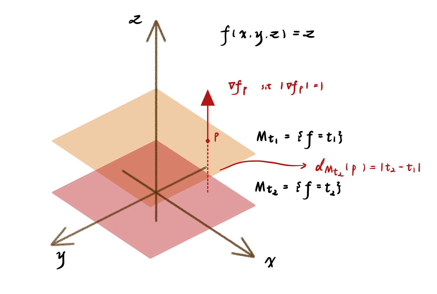
The operator and equation 1.6 naturally arise via the following geometric construction. Let be a Riemannian manifold. Suppose smooth and . Remember that we denote the Levi-Civita connection on and for a smooth function on a Riemannian manifold, we have
where is the total differential.
Notation 1.3.5.
We will abuse our notation and denote the by if there is no confusion.
Denote the -level set of . We know that for each , is a regular submanifold of codimension by the regular value theorem (). Since is smooth, by definition the gradient curve of satisfies . And we can see that along , increases with unit speed:
Thus for some constant .
Lemma 1.3.6.
The gradient curve is a unit speed geodesic.
Proof.
We will show this lemma by claiming that for a smooth function
| (1.8) |
Suppose 1.8 is true. Consider . If then by our construction, and . Therefore, and .
Since , then by 1.8, we know that is -Lipschitz, i.e.
On the other hand, by the definition of . Therefore, we have
So all the inequalities are equalities. Hence is a unit curve whose length is equal to the distance between its endpoints, and hence it’s a geodesic.
This means that the gradient curve is unit speed geodesic. Now we only need to show 1.8. Suppose that , take a unit speed geodesic from to . Denote . Then and . Then
On the other hand, if . Consider , then
By the definition of directional derivative, taking , then
which turns out that is not -Lipschitz. ∎
Now we conclude that if , then for any , the gradient curve starting at are unit speed geodesics normal to the level sets, i.e. . Moreover, the level sets are equidistant with respect to . Namely, for any point , the distance .
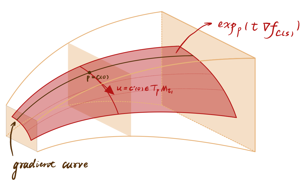
Remember in the theorem 1.1.2, we produce Jacobi fields by computing the variational field of the variation 1.2. Now we are particularly interested in the situation that the geodesic is the gradient curve of . Fix and , Let be a smooth curve in such that .
Remark 1.3.7.
Remember that the variation 1.9 is defined Jacobi field when the level set is complete or the interval of the geodesic is compact. And since we already define our geodesic over the interval we don’t need to worry about whether is complete or not.
Remark 1.3.8.
It immediately follows from Lemma 1.3.6 that where is the gradient flow of .
Because , along , is the unit normal to . Therefore by the Weingarten equation for a hypersurface (Theorem 8.13 in [Lee19])
where is the shape operator of . This tells us that the Hessian operator of is the shape operator of the level sets of .
We can differentiate along . Then, on the one hand,
| (1.10) |
On the other hand, by the Jacobi equation and ,
| (1.11) |
Therefore, combining 1.10 and 1.11,
where is a symmetric and bilinear form . Since we can choose an arbitrary initial vector perpendicular to the geodesic, we can conclude that
Therefore we always split the Jacobi equations of the Jacobi fields arising from variations of gradient curves of into two equations.
So the shape operator plays the role of as in the scalar Riccati equation 1.5.
Remark 1.3.9.
Let , then outside of , is smooth near and gradient curves are unit speed geodesics perpendicular to . Especially, consider the hypersurface . If is a compact embedded submanifold, then by the tubular neighborhood theorem, is diffeomorphic to . And if the normal bundle is trivial, separates locally, i.e. has two components.
In general does not separate locally when is not trivial. For example, consider the case when is a Mobius band and is a circle. does not separate locally.
Lemma 1.3.10.
Let be a complete Riemannian manifold and be a closed subset in . Let . Suppose is smooth on some open set . Then on .
Proof.
We prove it in a special case is a point. The general case can be proved using the first variation formula. Take and the unit speed geodesic started at . In the case when the initial condition is given, we can also solve by choosing appropriate . Just take so that is the gradient curve of such that . Then is smooth inside the injectivity radius, and more generally, outside of . We want to show . We first notice that is -Lipschitz by the triangle inequality.
On the other hand, because , then
implies all inequalities are equalities, thus . Since , and we have already known that , we must have .
∎
Given a unit speed geodesic with using function the above construction can produce any normal Jacobi field along with on where is smaller than the injectivity radius at . Indeed, let and let be a vector orthogonal to . Let be a curve in the unit sphere in with . Let and . then by construction and is a Jacobi field along with . Also by construction, we have that for any and for any fixed the curve is a gradient curve of . Note that here blows up as , more precisely as .
Remark 1.3.11.
More generally the above works inside the conjugate locus rather than the cut locus of . That is if is a (not necessarily shortest) unit speed geodesic with and there are no conjugate points along then such can be defined locally near and hence there exists on satisfying the Riccati equation (1.7) with initial condition .
Remark 1.3.12.
For later applications, we will also want to be able to guarantee the existence interval of with initial conditions . This can be accomplished as follows. Given a unit speed geodesic with and let where .
We will call such a geodesic submanifold defined by . Note that by construction the second fundamental form of at is 0.
We will say that there are no focal points of along if the normal exponential map to is a local diffeomorphism near . This condition guarantees the function defined locally near is smooth.
Then given by the second fundamental form of at solves the Riccati equation (1.7) along wit initial condition .
Chapter 2 Model Spaces, Hessian, Cosine Law
The key in the last lecture is to split the Jacobi equation
Next, we want to do comparison theory for these equations.
Let be a unit orthonormal basis at . We can extend to parallel vector fields along . Since we know the parallel transport preserves the orthogonality, we obtain an orthonormal frame along . This allows us to write the shape operator in the basis as a symmetric matrix . Then, the equation 1.6 can be rewritten as
which is a first-order matrix ODE system. Moreover, the second equation can be solved first, independently of the first equation.
This simplifies our problem. However, it is very difficult to solve this ODE system explicitly for the general Riemannian manifold. In fact, we will see soon that we can solve this matrix ODE explicitly for the spaces of constant sectional curvature. And we can develop our comparison theory based on that. When , we compare things to the equations in the model space , the simply connected space of . This section is the preparation of the comparison theory of the constant sectional curvature. We will first develop the trigonometry of the model space. This helps us to write the explicit expression of the Jacobi fields in the model space. Next, using these trigonometry functions, we can define the modified distance function so that we can have a scalar function version of the Hessian matrix.
2.1 Angles and Triangles in the Models Spaces
Definition 2.1.1.
Given a number , the define the -dimensional model -space to be a complete simply connected -dimensional Riemannian manifold of constant curvature . And the -dimensional model -space will be denoted by .
-
•
If , is isometric to a -sphere of radius . In particular, is the unit -sphere which is also denoted by .
-
•
If , is just the -dimensional Euclidean space which is also denoted by .
-
•
If , is the hyperbolic space rescaled by . In particular, is the standard -dimensional hyperbolic space denoted by .
Notation 2.1.2 (See [AKP22]).
We denote so that
Notation 2.1.3 (See [AKP22]).
The distance between points will be denoted by .
Notation 2.1.4 (See [AKP22]).
Let , a shortest geodesic segment connecting and will be denoted by .
The segment is uniquely defined for . For it is defined uniquely if . This is a strict inequality because when , we can think of and as the north and the south poles and there are infinitely many choices of the geodesic segments connecting these two points.
Definition 2.1.5 (Triangle (See [AKP22])).
We have two ways of defining triangles, one is by vertices and another one is by side lengths.
-
•
Triangle by Vertices: A triangle in with vertices is the ordered set of the three sides . In short, it will be denoted by .
-
•
Triangle by Side Lengths: A triangle in with side lengths will be denoted by .
Given , the triangle is uniquely defined as long as the segments are uniquely defined which happens iff . So means that are such that
For to be defined, the sides must satisfy the triangle inequalities
| (2.1) |
Conversely, given satisfying the triangle inequality, when can we find a triangle in with sides ?
Proposition 2.1.6.
Let satisfies the triangle inequalities 2.1. Then for , we can always find such a triangle and it is unique up to isometry. However if , the triangle exists if and only if
Moreover, if
the triangle is unique up to an isometry of .
Proof.
The case when is trivial. Suppose . If is defined, we can consider such that . By moving to the north pole by an isometry and extending to the south pole, we observe that

Similarly, we can also show
This means, if , then since otherwise, for example, if , we have thus, . Contradiction Uniqueness can fail when equality holds. For example, there are infinitely many geodesics of length connecting the north and the south poles.

∎
Definition 2.1.7 (Hinge (See [AKP22])).
Let be a triple of points such that is distinct from and . A pair of geodesics will be called a hinge and will be denoted by
Notation 2.1.8 (See [AKP22]).
Let be a triangle in . Then the angle at will be denoted by . Notice that is also the angle of opposite to . In this case, we will write
where the functions and will be called respectively the model side and the model angle.
2.2 Trigonometry of the Model Space
Consider the model space . Let be a unit speed geodesic, i.e. for each . We want to solve for the explicit expression for the Jacobi fields perpendicular to the geodesic, i.e. . Because the model space is the space of constant curvature , we can choose a unit vector perpendicular to , and extend to a vector field along obtained by parallel transport. In particular, . Obviously, and for all .
We can set so that we only need to solve for to find the explicit expression of in . Since space is the space of constant sectional curvature . Then by Proposition 8.36 in [Lee19],
Thus, for any vector fields along ,
Therefore, and we can rewrite the Jacobi equation as
Remember that is parallel, therefore , and we have
Thus, we conclude that is a Jacobi field if and only if
| (2.2) |
for each . By solving , we can find the explicit expression of the Jacobi fields in the model spaces.
Remark 2.2.1.
Remember from the last lecture, that we can derive the scalar Riccati equation from 2.2. When , we can derive 2.2 from any Jacobi field of any -dimensional manifolds. For , we can derive the scalar Riccati equation only for model spaces. For general manifolds in higher dimensions, we can only have matrix Riccati equations.
The general solution, as a second-order constant-coefficient linear ODE equation 2.2, is
Under the initial condition and , The explicit solution of 2.2 is denoted by such that for any ,
| (2.3) |
where
On the other hand, under the initial condition and , the explicit solution of 2.2 is denoted by such that for any ,
| (2.4) |
where
In terms of the and , we can rewrite the general solution of the equation 2.2 as
so that the Jacobi field in can be written as
We will call and the cosine and sine functions of the model space .
A straightforward computation gives us the laws of the trigonometry functions in the model spaces,
Remember that we used the replacement to derive the scalar Riccati equation . When , then is the model cotangent function which is denoted by . Then the Riccati equation can be written as
This can also be easily checked by a direct computation. Similarly, if we take which also solves 2.2 then also solves the Riccati equation .
2.3 Hessians Operator
In order to compare the Hessian operator of a general Riemannian manifold with those of the model spaces, we need the following explicit expression of the Hessian operator in the case of model space.
Proposition 2.3.1.
Let , . Take a unit speed geodesic starting at with . Denote by , then
is defined for any with and is the orthogonal projection onto the tangent space of the sphere centered at of radius .
Proof.
Let be a normal Jacobi field along such that . Remember that we have already know that we can split the Jacobi equation into
and the Riccati equation. Because the shape operator along is just the Hessian matrix. This is
| (2.5) |
Let be a parallel orthonormal frame along and in particular we take for . It is easy to check that for each , the vector fields
are also normal Jacobi fields along for some constant . Then
| (2.6) |
On the other hand, by the above equality 2.5, by the linearity of the Hessian operator, we have
| (2.7) |
As the right hand sides of the equation 2.6 and 2.7 are equal, we have
On the other hand, since . Then, as is linear, we have
| (2.8) |
Thus, in terms of the basis , the explicit expression of is
∎
Since this can be rewritten as
Therefore, under the basis we can write as the following matrix.
2.4 The Cosine Law for Model Spaces
In this section, we want to derive the cosine law for the model space. The key point here is to obtain a scalar Hessian at every point of the model space (instead of just on the equidistant sphere of ) by changing to via some smooth function . Namely, we want
| (2.9) |
for each with . And is some scalar-valued function over . Denote , if we have 2.9, then for any , and any unit speed geodesics in (not necessarily passing through ), we can easily compute the second-order derivative along any unit speed geodesic. Indeed, remember the step 2.8
2.4.1 Modification Function
We define the modification function by
| (2.10) |
Then the explicit expression for is
where in particular when ,
Corollary 2.4.1.
By the formula 2.10, it is not hard to check that solves the following initial value problem:
| (2.11) |
2.4.2 Scalar Hessian Operator
Let , the distance function from is . We will call the modified distance function to . It turns out that plays the role of the function in 2.9.
Theorem 2.4.2.
The Hessian of is scalar. Namely,
| (2.12) |
at each .
Proof.
Recall the Hessian formula [Lee19], for any ,
for any smooth functions and . Setting and . Along a unit speed geodesic starting at , since , for , we have
which followed by definition and the law . Then since along and , we have
because for . On the other hand, since ,
The second term vanishes due to so that . Therefore, we can conclude that using the modified distance function , we have
∎
Corollary 2.4.3.
Remark 2.4.4.
Unlike , the modified distance function is smooth at .
2.4.3 The Cosine Law in the Model Space
The above corollary 2.4.3 is essential to derive the cosine law in the model space . To do that, we introduce the follow notations for metric spaces.
Definition 2.4.5 (Model Angle).
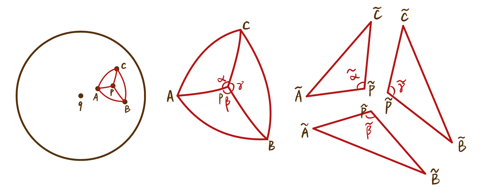
Let be a metric space, and is defined and , then the angle measure of at will be called the model angle of the triple at and will be denoted by
Definition 2.4.6 (Hinge Angle & Model Side of Hinge).
Let be a metric space, . Let be a hinge, then we can define the hinge angle of the hinge as
for and if this limit exists. And we can define the model side of the hinge as
Fix such that is a triangle uniquely defined in the model space . Then we can write and .
Proof.
We define and it is easy to see from Figure 2.3 that .

Moreover, at , we have
Therefore,
Knowing and we can easily find by solving the IVP for the equation . This allows us to find and hence also which yields the cosine law in .
Theorem 2.4.8.
In , the formula of and can be written as the cosine law in :
Proof.
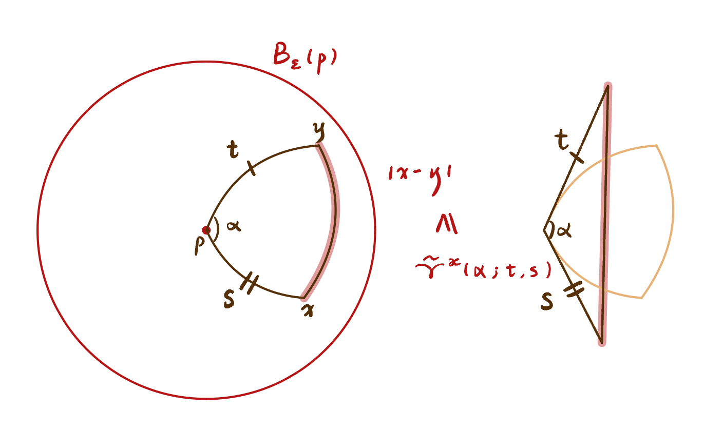
Here we only compute the case when . Given and a unit speed geodesic starting at as in Figure 2.4

We define . The question is to find . It is easy to see that . Then and . Therefore, denote , by solving the IVP
we can derive the cosine law for , i,e.
∎
2.5 Hessian Comparison Theorem
The cosine law is essential to the theory of comparison geometry. And it is very important for proving Toponogov’s comparison theorems. The key to proving the cosine law in the model spaces is the identity 2.13 for the Hessian operator for . In this section, we are going to compare this operator to the Hessian operator of the modified distance function for Riemannian manifolds of sectional curvature bounded below via the following theorem.
Theorem 2.5.1 (Hessian Comparison Theorem).
Let be a Riemannian manifold such that . Fix , let . Then for or more generally outside of the cut-locus of , we have
| (2.14) |
Let be a Riemannian manifold, and a unit speed geodesic starting at . By the theorem 1.3.4, we can use a symmetric operator along the geodesic to split the Jacobi equation:
Let be a normal unit vector field parallel along . We use to denote . Let . Then by the Riccati equation and the fact that is symmetric, i.e. ,
where and .
By Cauchy Schwartz: , we can conclude that
That is
| (2.15) |
Lemma 2.5.2.
if we have
and . Then,
-
•
if for ;
-
•
if for ;
Proof.
Take the subtraction, then
Take , then we have
Multiplying both sides by then
Therefore, is non-increasing. If , then and hence for , or equivalently for . Similarly if , then and hence for i.e. for . ∎
Corollary 2.5.3.
Let , consider
Then
For some . Apply what we just discussed, then
-
•
If for ;
-
•
If for ;
Therefore, for Riemannian manifold of sectional curvature bounded below, i.e. , for all . Hence for , by 2.15, we have
we can now compare it to what we obtained in , i.e. . Especially, we need to be careful with the blowing up case when as , which happens when and . This is because for on , the shape operator as . In order to address this case, we need the following lemma.
Lemma 2.5.4.
Let satisfies
-
•
;
-
•
Then for all for which is defined
Proof.
Suppose not. that is such that . This implies such that by the continuity of . Define . It satisfies
where . Thus by the above discussion, we have
Now we have the contradiction: is finite over .
contradiction. ∎
Now we can prove the Hessian comparison theorem.
Proof of the Hessian comparison theorem 2.5.1.
Let be a unit speed radial geodesic starting at . Let be the shape operator of the sphere at . Let be a unit normal vector field parallel along . If we take , then satisfies and . By the lemma 2.5.4, we have . Since , then
Therefore, where is the projection map to . Recall that on . And in the direction parallel to we have that both and .
As we explained before, along any other unit speed geodesics in the with , because
it holds that
Chapter 3 Local Comparison Theorems
3.1 Rauch Comparison Theorem
Theorem 3.1.1 (Rauch () Comparison Theorem).
Let be a Riemannian manifold, . Let be a unit speed geodesic, i.e. . Let be a normal Jacobi field along . We will also denote by a unit speed geodesic in and by a normal Jacobi field along . Suppose one of the following holds
-
•
Rauch : and and there are no conjugate points to along on ; or
-
•
Rauch : and and there are no focal points along on for the geodesic submanifold defined by ;
Then is non-increasing. And on .
Remark 3.1.2.
The conclusion of the theorem implies that in both cases of Rauch I and Rauch II, the first zero of (if it exists) must occur before the first zero of . In our applications Rauch I will only be used for shortest geodesics in which case the no conjugate points assumption is always satisfied.
Proof of Rauch Comparison Theorem .
Let us treat Rauch I first.
As before, we denote by the shape operator of . By Remark 1.3.11 the assumption that there are no conjugate points along guarantees that is smooth on and as .
Recall that we can convert the Jacobi equation of and to
| (3.1) |
with initial conditions and and as .
Look at
Therefore, we proved
| is non-increasing | |||
| is non-increasing by the monotonicity of |
By our assumption, (using L’Hopital’s rule), then . Because it goes down, the first zero of occurs before the first zero of . This proves Rauch .
The proof of Rauch is very similar. We only indicate the differences.
Take a hypersurface containing and such that and its second fundamental form is zero at . For example one can take to be the image under of a small ball in . Then set to be the shape operator of of the -sphere around at . Then the comparison argument is the same except we get and the equality holds in the . Then the initial conditions for system (3.1) become and . The rest of the proof is the same except we don’t need to use L’Hopital. ∎
Remark 3.1.3.
The above proof only works so long as there are no conjugate points (Rauh I) or focal points (Rauch II) along . In particular, it means that in either case is not zero on . Nothing can be said after the first zero of .
Proposition 3.1.4 (Rigidity Case of Rauch Comparison Theorem).
Under the assumptions of Rauch comparison if there is a positive such that then on and moreover there is a parallel normal vector field along such that on it holds that
-
•
Rauch : ;
-
•
Rauch : .
Proof.
We will only give proof for Rauch II, the proof for Rauch I is similar. Without loss of generality .
Suppose and for . Then by monotonicity of we have that for all .
The proof of Rauch comparison gives that and before the first zero of .
If the inequality is strict at any point then the proof gives that which we know is false.
Recall that if a symmetric matrix satisfies and for some nonzero vector then is a -eigenvector of , i.e. .
Hence for any . But which means that on . Let be parallel along with and Let . Then also satisfies on . Hence both and satisfy the same first-order IVP and hence on .
∎
3.2 Berger Comparison Theorem
We are going to introduce the Berger comparison theorem [Ber62] in this section. This is useful in proving the concavity of the distance function. The following Berger comparison theorem is an important implication of the Rauch comparison theorem.
Theorem 3.2.1 (Berger Comparsion Theorem (Figure 3.1)).
Let be a manifold with . Let be a (not necessarily shortest) unit speed geodesic in . Let be a unit parallel vector field along such that for all , . Let
Now, consider , , in the corresponding picture in the model space . Namely,
Then for all small it holds that
where
In the special case , the above estimate becomes
for all small .
Proof.
Use Rauch in 3.1.1. Since for any fixed the curve is a geodesic, is Jacobi along . Also, at , ad .
Notice that the last equality holds because is a parallel vector field. Thus, we know that and . Similarly, the above also works for . Then by Rauch , we have that
In particular, if , then the model space is just . Then is a straight line and a constant vector field along . Notice that we can write the straight line as a straight passing through , i.e. (WLOG we assume ) for some vector . Then
In this case, is constant in . In Rauch , is parallel along . By Berger’s comparison theorem 3.2.1,
∎
This immediately gives.
Corollary 3.2.2.
Suppose under the assumptions of Berger’s comparison is shortest and . Then for all small .
Moreover, for later applications we will need to understand the rigidity case in the above corollary.
Proposition 3.2.3 (Rigidity Case of Berger Comparison Theorem).
Then
is a totally geodesic flat isometrically immersed rectangle in .
Proof.
Recall that a submanifold is called totally geodesic if for each , there is a neighborhood of is mapped into via the exponential map of , i.e. . This is well known to be equivalent to the second fundamental form of vanishing.
And a Riemannian manifold is called flat if it is locally isometric to Euclidean space. This is well known to be equivalent to the curvature of this manifold to be identically zero,
By Berger’s comparison, we have that
However, we are given that which means that all of the above inequalities are equalities. In other words
| (3.2) |
In particular
In the proof of Berger’s comparison we have that for any small fixed we have and and similarly .
Hence the equality implies that for any . By the rigidity case of Rauch II with this implies that for any fixed the field is parallel along .
Moreover, since is also parallel along this curve we wee see that and are orthonormal for any . This immediately gives that the map is an isometric immersion.
It remains to be observed that this immersion is totally geodesic. We already know that . We will show that too.
Recall that we proved that
for any . Since for we also have that is unit speed for . Hence it’s a geodesic and therefore for any . This proves that the map restricted to this rectangle has trivial second fundamental form and hence is totally geodesic.
∎
3.3 Local Toponogov Comparison Theorem
The most important corollary that we are introducing now is the hinge version of the Toponogov comparison theorem, which is further equivalent to the angle version of the Toponogov comparison theorem.
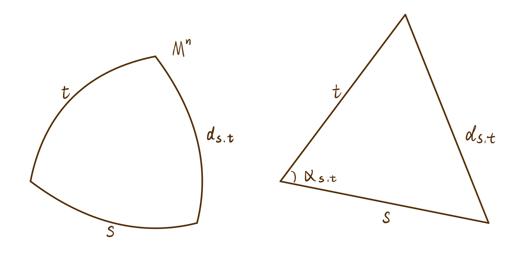
Theorem 3.3.1 (Local Toponogov Hinge Comparison).
Let be a Riemannian manifold of . Fix . There is a small such that the following holds. For any we have
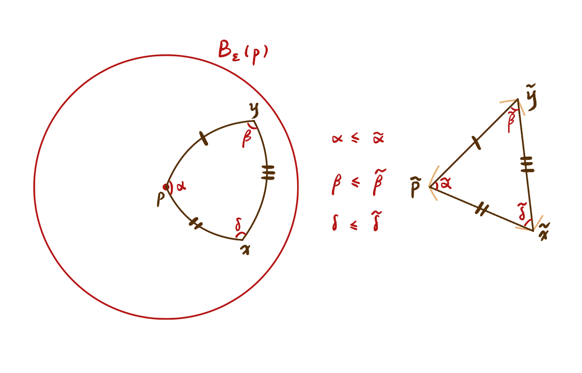
Theorem 3.3.2 (Local Toponogov Angle Comparison).
Let be a Riemannian manifold of . Fix . There is a small such that the following holds. For any and the comparison triangle , we have
We are going to argue that the two versions of local Toponogov comparison theorems are equivalent.
Proof (Local Hinge Comparison to Local Angle Comparison).
We only need to prove and the same argument works for the other two angles. The key observation is that is monotone in creasing on and hence by the cosine law in the model plane the map is monotone increasing for any fixed .
Suppose the hinge comparison holds. Consider the triangle in and denote , and . We also define . Similarly, we define . On the other hand, consider the triangle . Then by the hinge comparison,
By its definition, we know that , and . Now by the cosine law, we know that
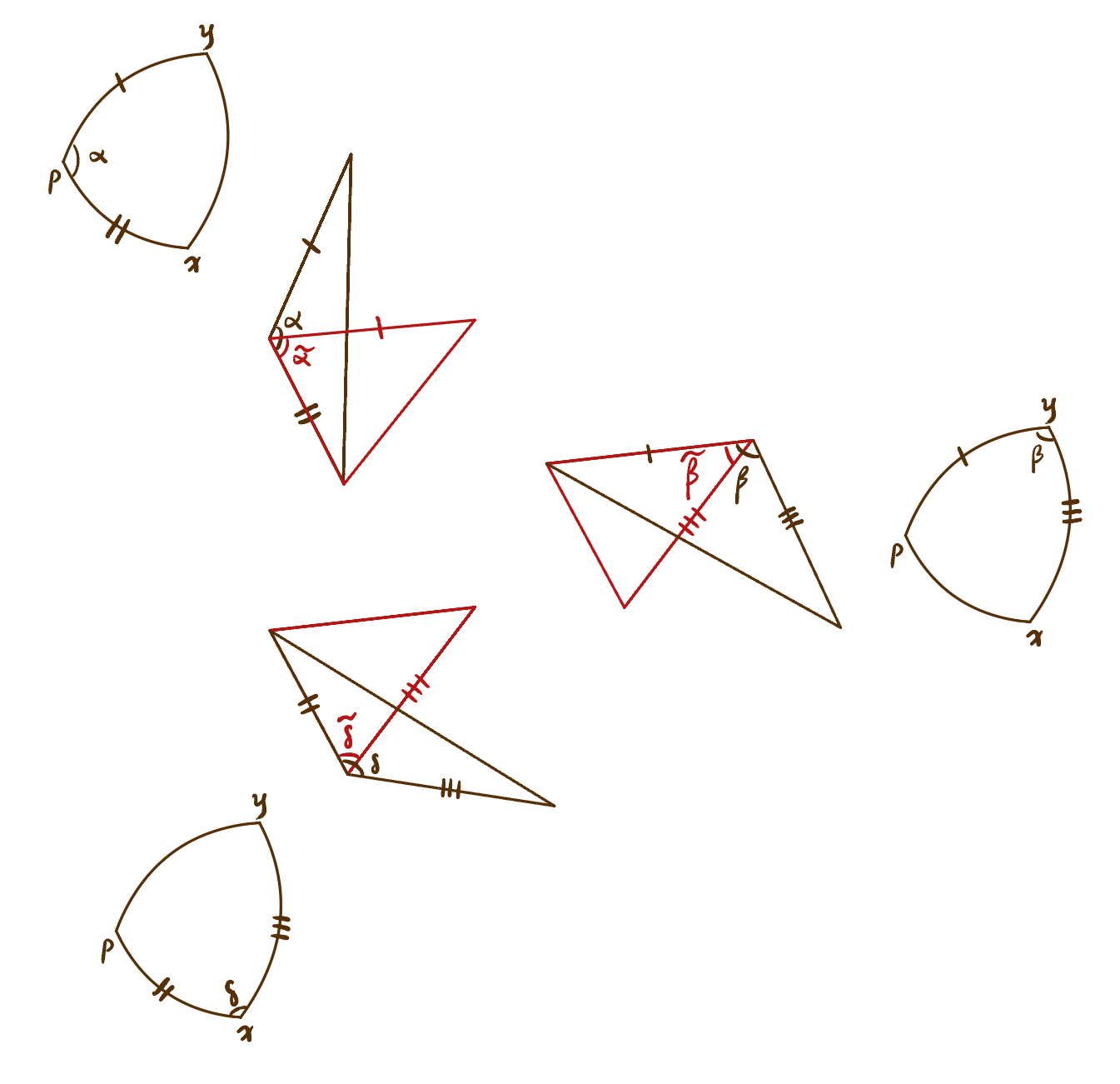
It is also easy to see that the local angle comparison implies the local hinge comparison. The arguments are the same and the key point is still the cosine law. ∎
Now we relate the local Toponogov theorem to Rauch comparison theorem
Theorem 3.3.3.
Rauch comparison implies the hinge comparison
Proof.
To show how Rauch comparison implies local hinge comparison. Take and . Notice that both and are diffeomorphism near and respectively.
Especially in , we know that is a diffeomorphism near , we can pull back the Riemannian metric from to , i.e where is the Riemannian metric of . Take some isometry . Consider the map
and the map
It is easy to see that
because by construction is an isometry from to . Notice that it is easy to see being -Lipschitz is equivalent to the hinge comparison because for any geodesics starting at , their length, and the angle between them are preserved by .
Therefore, we only need to show is -Lipschitz. Here we only consider the case when and in this case, and . And in this case, we just need to show is -Lipschitz on a small neighborhood of . We need to show that for and ,
This is obvious for radial vectors, i.e. . Because the exponential map is an isometry, in this case, for general , we can decompose . where for some is pointing to the radius direction. Then we have
Recall that by the Gauss lemma, a geodesic starting at is perpendicular to a small sphere near for some small . Then by the Gauss lemma, we notice that
Therefore, by the Pythagorean theorem, we have
It is sufficient to show
Recall the explicit construction of the Jacobi field vanishing at the initial point (see theorem 1.1.6). For and along , we have
We denote the corresponding Jacobi field in the model space. In our case, thus . By the Rauch , we get that
∎
Exercise 3.3.4.
Show that a Riemannian manifold satisfies if the local angle comparison holds. hint: This follows from the Taylor expansion formula in Meyer’s Notes (see [Mey04])
What if we reverse the inequality in our angle comparison theorem? i.e. Is that correct that if the angle comparison holds (At least locally) with appropriate inequality? The answer is YES! However, our proof DOES NOT work in this setting. The recall what we did for lower curvature bound
Consider along where is the shape operator of the equidistant hypersurface and the unit normal vector field of the hypersurface. Let be unit parallel vector fields along . If , then . Look at . Then
by the Cauchy-Schwartz inequality, i.e . Also, because , we can conclude that
This allows us to reduce the study of the matrix Riccati to the scalar Riccati inequality . However, this trick does not work for . In that case, we need to deal with the Ricatti inequality . Here the above trick using the Cauchy-Schwartz inequality doesn’t work and one has to study the matrix Riccati inequality directly. This can be done with the help of the following result. We omit the proof as in this notes we are only interested in applications to lower curvature bounds.
Theorem 3.3.5 (See [EH90]).
Let be smooth with . For let be a solution of
with maximal . Assume that . Then and on
Then the angle comparison for the upper curvature bound can be explained by the following general Rauch comparison theorem.
Theorem 3.3.6 (General Rauch and Rauch Comparison).
Let and be two Riemannian manifold along their geodesics and . Assume that
for any normal unit vector fields along . Let be Jacobi fields along for . Suppose either
-
•
Rauch : Assume that has no conjugate points on , and ; or
-
•
Rauch : Assume that has no focal points on , and .
Then is non-increasing up to the first zero of .
3.4 Other Local Comparison Theorems
We studied the two versions of local Toponogov’s comparison theorem (local angle comparison and local hinge comparison) holding in a small ball where . In this lecture, we are going to introduce a few more comparison theorems that are equivalent to the angle comparison and the local hinge comparison theorem.
3.4.1 Monotonicity of Angle Comparison
Theorem 3.4.1 (Local Monotonicity of Angle Comparison).
Let be a Riemannian bounded from below. For any there is a small such that the following holds. Let . Let , be unit speed parameterizations of respectively. Let . Then the model angle is monotonically non-increasing with respect to both and .
In this section, we mainly want to show the local monotonicity of angle comparison is equivalent to the local angle comparison. The key lemma used in proving the local angle comparison implies the local monotonicity of angle comparison is Alexandrov’s lemma.
Lemma 3.4.2 (Alexandrov’s Lemma).
In , let and consider the following picture where the triangles and is uniquely defined. We also marked the angles in the picture. Assume
-
•
;
-
•
And if , assume . 111This assumption is necessary since we want the triangle to be uniquely defined up to isometry.
Now consider the triangle and the angle in the following picture, we claim that .

Proof.
We extend the side of length by length to point . We also marked the point in the picture below.
![[Uncaptioned image]](/html/2404.09792/assets/comparison_images/lec5image/IMG_2095.jpg)
Denote . Now it is easy to see that by the cosine law.
![[Uncaptioned image]](/html/2404.09792/assets/comparison_images/lec5image/IMG_2097.jpg)
Next, still by the cosine law, by reducing to in the picture above, we got . ∎
Theorem 3.4.3.
Proof.
Suppose the angle is monotone with respect to and , then (see [AKP22])
| (3.3) |
since is infinitesimally close to , and we can show this using Taylor expansion formula for in Meyer’s notes [Mey04].
Therefore for any .
Conversely, suppose the local angle comparison theorem holds. Consider the following picture,
![[Uncaptioned image]](/html/2404.09792/assets/comparison_images/lec5image/IMG_2100.jpg)
3.4.2 Point-on-a-side Comparison
Theorem 3.4.4 (Point-on-a-side Comparison).
Let be a Riemannian manifold with . Let be positive numbers such that satisfies the triangle inequalities such that there exists a triangle in the for some small and (See Figure 3.8). We claim that , where is the length in and is the length in .

Theorem 3.4.5.
The point-on-a-side comparison is equivalent to the monotonicity of angle comparison.
Proof.
Suppose the monotonicity of angle comparison holds, we can extend side as in the following picture.
![[Uncaptioned image]](/html/2404.09792/assets/comparison_images/lec5image/IMG_2102.jpg)
Draw the triangle and extend the by in so that we can obtain a new triangle . We denote . On the other hand, we extend the side of the triangle by directly in so that we can have the triangle . Compare with , by the monotonicity of angle comparison, we have
By the cosine law, this implies that . Sending , so that and , we can conclude that which is the point-on-a-side comparison. The converse direction is similar. ∎
3.4.3 Four-points Comparison
Theorem 3.4.6 (Four-points Comparison).
Let be a Riemannian manifold such that . Fix and consider quadruple of points for some small . We draw the following picture.
And we assume all comparison triangles exist and are unique. This is automatic if is sufficiently small. Then for in their corresponding comparison triangle, i.e.
Then,
Theorem 3.4.7.
We want to show that the four-points comparison 3.4.6 is equivalent to the angle comparison.
Proof.
We take three initial vectors of starting at . They belong to the unit sphere . Because , then we have
![[Uncaptioned image]](/html/2404.09792/assets/comparison_images/lec5image/IMG_2104.jpg)
Then by the angle comparison, since , we derive that
Conversely, we instead prove the four-point comparison implies the monotonicity of the comparison angle. We draw the following picture, so that is also in a straight line, thus .
![[Uncaptioned image]](/html/2404.09792/assets/comparison_images/lec5image/IMG_2105.jpg)
Therefore, by the four-points comparison, . Then by Alexandrov’s lemma, we can conclude that the comparison angle satisfies . ∎
Remark 3.4.8.
The four-points comparison involves only distances in . This allows it to be used to give a metric definition of lower sectional curvature bound. It is also clear that it behaves well with respect to most notions of convergence of metric spaces. We will see later that it is stable under Gromov-Hausdorff convergence.
Remark 3.4.9.
In this section, we have established the equivalence of various local versions of angle comparison including the four-points comparison. Equivalence of global versions of these comparisons also holds but for some implications require the globalization theorem. For the local proofs directly generalize to global ones.
3.4.4 Point-on-a-side Comparison by Jensen’s Inequality
In this section, we want to study Jensen’s inequality of and give a new proof of local point-on-a-side comparison 3.4.4. Remember we already proved that if in where . Then near (or more generally, outside of cut locus of ) satisfies
as a matrix. Equivalently, for any unit speed geodesics in a small ball around (or more generally, outside of cut locus of ) it holds that
| (3.4) |
In the model space the inequalities above are equalities, in particular .
Example 3.4.10.
For example, when , if , then satisfies 2.11, therefore . Then along any geodesic , we have . And for , , we have
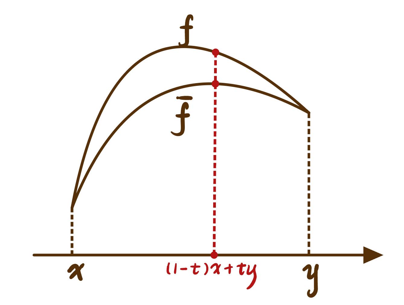
In this section, we are going to justify that the above result of the modified distance function gives a different proof of local point-on-a-side comparison 3.4.4. To show this we need to understand the inequality 3.4 geometrically. Let be a smooth function, fix , and suppose it satisfies
We want to understand this condition geometrically. Firstly, we consider the simple case when , then is easy to understand:
| is concave. |
Denote , since is concave, then for , by definition, we have
In terms of , this is
| (3.5) |
the concavity inequality of . Notice that the concavity inequality 3.5 is equivalent to Jensen’s inequality, which says that if is a function that satisfies , then for any function satisfying and and , we have
That means the graph of the comparison function is below the function .
Remark 3.4.11.
The above can be plus some affine term for some constant .
Now let’s consider the case when so that
| (3.6) |
Then we want to derive a similar Jensen’s inequality as above,
Lemma 3.4.12 (Jensen’s inequality).
Suppose inequality 3.6 holds for some . Let such that (note that this is only a restriction if ). Fix satisfying and and . Then on , i.e. for any , we have the Jensen’s inequality
Proof.
Let us first prove the lemma under a slightly stronger assumption .
Suppose the conclusion of the lemma is false. Namely, there exists such that
| (3.7) |
Because and ,
Denote . We have and . Therefore, our assumption 3.7 in terms of becomes
Suppose .
Let be value minimizing , then and . Notice that since , then . When ,
which contradicts to .
Let us now consider the case . By rescaling it is enough to consider the case .
Thus we are assuming that satisfies and . We will use the following -trick: Since we can find an such that on (translation if necessary). Note that solves and on . Still, we denote . Then on .
Denote on then there exists the minimizing point such that
Then by the second order derivative test, we have and . Notice that
Then, since
by substituting and using that , we have
This contradicts the assumption that .
The case of weaker assumption can be proved via approximation. We take for arbitrary small , then
Then we obtain Jensen’s inequality
for some . And since is arbitrary, we can prove Jensen’s inequality for as well. ∎
We are going to show the above Jensen’s inequality gives a different proof of the point-on-a-side comparison in .
Proof.
This is a new proof to the point-on-a-side comparison 3.4.4. Consider the following picture, fix and and and the geodesics parameterize the opposite sides of and .
we denote and . Then along and along . Since and , by Jensen’s inequality 3.4.12, we can conclude that for each on and its corresponding point in the model space. Then, since is monotone increasing, we can conclude that . ∎
Chapter 4 Global Toponogov Comparison Theorems
In this lecture, we will prove the global Toponogov comparison theorem via the key lemma (Remember that we only proved the Toponogov comparison theorem on ).
4.1 The Key Lemma
Theorem 4.1.1 (The Key Lemma).
Let be complete and , , and such that if the comparison
hold for any hinge satisfying
| (4.1) |
Then the comparison
hold for any hinge satisfying
| (4.2) |
This key lemma allows us to extend the hinge comparison from small hinges to bigger hinges. We want to prove this key lemma via contradiction. Firstly, we assume the local hinge comparison fails 3.3.1 for a hinge satisfying 4.2, i.e.
| (4.3) |
Notice that .
Our idea is to construct a sequence of smaller and smaller hinges satisfying 4.4. And at the limits, the hinge admits the length in 4.1, which is impossible because we cannot have both and .
4.1.1 Step 1: The Construction of a Smaller Hinge
Equivalently, we can modify the assumption 4.4 a little bit. Suppose there exists a hinge such that
| (4.4) |
We want to show that we can find a smaller hinge such that the comparison still fails. WLOG Suppose . Our first step is pick such that
It is easy to see such exists. Denote the geodesic such that and , we want to take for some . Look at
a continuous on . At , we have
Therefore, by the intermediate value theorem, there exists such that and we denote as . Note that .
Now we draw the comparison triangle . Then we can extend beyond to such that . denote
![[Uncaptioned image]](/html/2404.09792/assets/comparison_images/lec6image/IMG_2113.jpg)
Claim 4.1.2.
The hinge comparison fails on the smaller hinge , i.e.
Proof.
For and , we can check that
Thus, the the hinge comparison holds for both and , i.e.
We draw the following picture and annotate the length of each side.
Also, for opposite sides, we denote
![[Uncaptioned image]](/html/2404.09792/assets/comparison_images/lec6image/IMG_2116.jpg)
It is easy to observe that both and indicate the length of the side , thus . By the cosine law, we have both and . Therefore, we have
And by the assumption 4.4, we can conclude that . That means we can construct a “smaller hinge” where the hinge comparison fails. ∎
4.1.2 Step 2: Construction of a Sequence of Smaller Hinges
In this step, we repeat our construction. We denote by , by , by , by . Then we can construct a smaller hinge from .
-
•
If , then again, we take such that
-
•
If , then we take such that
By continuing this process, we will construct a sequence of hinges and a corresponding sequence such that
4.1.3 Step 3: How Far This Process Can Go?
The question now is how far this process can go. We are going to discuss this in cases:
-
•
Case 1: If there exists some such that the hinge satisfies
Then by assumption, the hinge comparison holds, i.e.
(4.5) However, the contradiction happens because
But 4.5 is equivalent to .
-
•
Case 2: If the Case 1 doesn’t happen, consider the sequence . Notice that is non-increasing and the limits . Moreover,
It is not hard to check that all the sides of the triangle remain bounded away from for large , i.e. we can find such that
(4.6) Let’s explain why 4.6 is true for some large . For example, if we have admits . Since and
Then , and by triangular inequality . Still by triangular inequality, . Then since
it is easy to compute that and . Therefore we have 4.6 holds for .
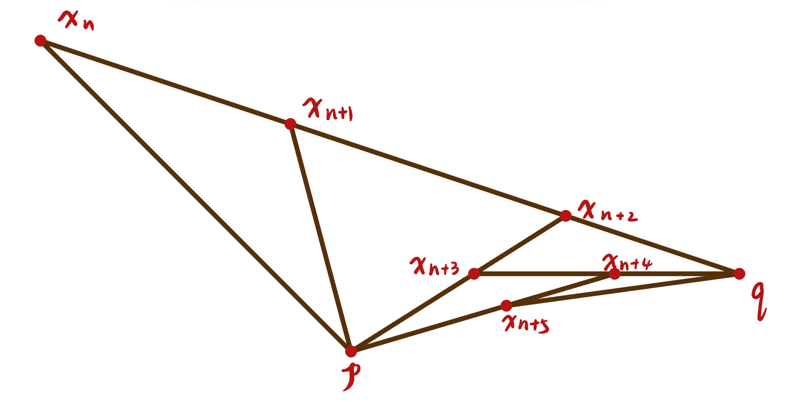
Figure 4.1: For example, if , we can pick the point such that 4.6 holds. We can also check that the sides and are approximately the same, i.e. . Use that and . This implies that . If is very small then is impossible because .
Consider the triangle of all the sides and . In the model triangle . Here (recall that , else we switch the roles of and ) But we also know that because
Thus as well. Therefore, . That means . Therefore,
But recall that
So we have the contradiction.
Now we finished the proof of the key lemma.
Remark 4.1.3.
The techniques in this lemma can be generalized to Alexandrov spaces because they do not depend on Riemannian geometry, see [AKP22].
4.2 The Global Toponogov’s Comparison
In this section, we want to generalize the various local Toponogov comparison theorems to the entire manifolds. We will present an argument in a simplified situation of compact and . For the proof in general cases see [AKP22].
Definition 4.2.1 (Comparison Radius).
Let be a compact Riemannian manifold with . For , we define the comparison radius at as
We know that for any since the Toponogov comparison theorem holds locally. In fact, if is compact, then
| (4.7) |
This is because for any such that converges to , there exists a the subsequential limits of . Since near , the comparison holds. Then for all large in the subsequence.
Remark 4.2.2.
Suppose and . Suppose for simplicity that , For , is the smallest possible. Then by applying the key lemma 4.1.1, the comparison will hold for all hinge of size because . This implies a contradiction. In general, take large so that is very close to , if we take for some fixed small , then for all large .
To finish the proof for one also needs the Short Hinge Lemma [AKP22] to deal with hinges longer than .
Also, for the perimeter of any triangle in the model space does not exceed . Hence the global Toponogov theorem proves the comparison for triangles of perimeter . Is this a serious restriction? We will see that, in Lemma 4.3.3, the answer is No!
4.3 The Global Functional Toponogov Comparison Theorem
4.3.1 Myer’s Theorem
Let’s start this chapter with the following famous result due to Myer [Mye35].
Theorem 4.3.1 (Myer).
Let be a Riemannian manifold with , then
Proof.
Suppose this theorem fails for some with , by rescaling, we can assume , so that and . Then there exist such that for some small . Let be the midpoint, i.e. . Let be a unit vector perpendicular to the geodesics , Denote .
Claim 4.3.2.
We claim that
for small .
By this claim, is no longer the shortest, so we have the contradiction.
To prove this claim, we want to apply the hinge comparison to the , so that
| (4.8) |
To check the perimeter condition holds, we first notice that and , by triangle inequality,
Thus the perimeter when and are small.
Lemma 4.3.3.
If has , then for any triangle in , we have
Proof.
By rescaling assume . Suppose this lemma fails for some triangle in , i.e
Then, there exists such that
So that for sufficient small, we can find
Now, we can do comparison for with the comparison triangle . It also holds that
which means almost lie on a great circle in . Moreover, this means we can find almost opposite to . By point-on-a-side comparison, , so
since and are very small. Now the contradiction rises since due to Meyer’s theorem. ∎
4.3.2 Functional Global Toponogov Comparison Theorem
Recall that we proved if with , let , denote . Near it satisfies
We want to say that this holds globally so that we can globalize Jensen’s inequality 3.4.12 and prove the global version of the point-on-a-side comparison. However, need not be smooth outside of the ball of the . Therefore, we need to interpret the above inequality appropriately in the region where for
Let be a function that we want to understand. Remember the derivative in general sense is also denoted by such that for all ,
Let . We want to understand the inequality
The simplest case is when then in the general sense.
Definition 4.3.4 (-Concave(Convex)).
is -concave(convex) or () in the general if is concave (convex). In other words, satisfies
for any .
Corollary 4.3.5 (Jensen’s inequality).
Let be -concave. Then for any such that in the general sense, and , it holds that
on .
Definition 4.3.6 (Semi-concave(convex)).
is called semi-concave(convex) if , , such that is -concave(convex).
Lemma 4.3.7.
If is -concave(convex), then is locally Lipschitz on , i.e. for any , there is a constant and an closed interval contains such that
for all .
Proof.
We can prove this for convex functions, then the same applies to concave functions by adding the negative sign. Fix and let be arbitrary points in . Take such that
Firstly, we claim that for a function that is convex on , it is also locally Lipschitz. It is not hard to show that that a convex function is bounded on any closed subinterval of . Hence, there exists such that
for all . Take a fixed and define . It follows that and , and by the convexity
Hence,
Switching the variable we get
This implies,
where .
And for an -convex function we have that is convex and hence by above it is locally Lipschitz on .
Hence is Locally Lipschitz as well.
∎
Theorem 4.3.8.
The following are equivalent for .
-
1.
is -concave;
-
2.
in generalized sense, i.e. , we have
if were smooth, then by integration by parts
In particular, when ,
-
3.
Barrier Inequality: , there exists open interval and such that , and on . If , then is linear.
Proof.
comes from smoothing by convolutions. We observe that if a sequence of -concave functions point-wise convergent to and convergence to . Then is -concave function immediately from the definition. We can use the following: If is concave, then can be approximated locally uniformly by a sequence of smooth functions, i.e. be a sequence of smooth bump functions converging to delta function so that is approximated by . Since in the usual sense, in the generalized sense. ∎
Remark 4.3.9.
Note the equivalence in the theorem 4.3.8 implies that -concavity in the sense of Jensen’s inequality can be checked locally. That is, to check that is -concave on it is enough to show that for any there exists such that Jensen’s inequality holds on . Then Jensen’s inequality holds globally. This follows because (2) can be checked locally using partition of unity. Indeed. Let be smooth with compact support. Then by POU, we can write where . Moreover, we can choose the partition of unity so that is small enough so that (2) holds on for every . Then
also.
This verifies that holds on .
It is immediate from definition that if we have a family of -concave functions such that
Then is also -concave on .
Proposition 4.3.10.
If is semi-concave and is smooth and . Then is also semi-concave.
Proof.
It is sufficient for us to prove is locally -concave for some constant. By directly taking the derivatives, we have
| (4.10) |
By the smoothness of , we know that there is a local bound for and . By Lemma 4.3.7, we know that is locally bounded and locally Lipschitz. Thus, first term is locally bounded. On the other hand, we know that also has a local bound above since is semi-concave. Since and is locally bounded this gives that is locally bounded above. This argument works if is smooth. For general semiconcave the result then follows by approximation. ∎
Remark 4.3.11.
The above proposition also holds if we replace the assumption with being semi-concave and .
Definition 4.3.12.
Now if , is -concave (satisfies ) if Jensen’s inequality holds, i.e. such that if take satisfies
and . Then on . (We are not assuming that is smooth) Indeed, we assume that is semi-continuous.
Recall that we proved that if is smooth, then . This justifies the above definition.
Theorem 4.3.13.
Let be LSC(lower semi-continuous). Then the following are equivalent.
-
•
in the above sense of Jensen’s inequality.
-
•
in generalized sense, i.e. , ,
-
•
Barrier Inequality: , then where is an open interval and if and , , on . And solves exact equation .
Remark 4.3.14.
We have some comments. If on and
| is -concave functions. -concave functions. |
is semi-concave in particular locally Lipschitz on .
-
•
As before if , are concave functions on ,
then is again concave follows from Jensen’s inequality.
-
•
If pointwise, and is concave and and . Then is -concave.
-
•
Let , then -concavity can be checked locally because n in generalized sense if local.
Definition 4.3.15.
Let be a complete Riemannian manifold, then is -concave if for any geodesics , is -concave. Moreover, is -concave if for any unit speed geodesic , is concave.
Theorem 4.3.16.
Let be complete and , , . Then is -concave if on . ( need not be globally smooth.)
Proof of Theorem 4.3.16.
We only need to check the Jensen’s inequality. By Toponogov,
for and since is monotone, then
This implies that is semi-concave on since
Therefore, is -concave. Thus it is semi-concave. Therefore is also semi-concave on . ∎
Remark 4.3.17.
The last result holds on any complete Riemannian manifold. That is if is complete and then is semi-concave on .
Chapter 5 Appliction of Toponogov’s Comparison Theorem
5.1 Curvature bounds and Topological Complexity
There are many results when the curvature bound implies a topological bound. In this section, we introduce the work of Gromov on bounding topological complexity (growth of the size of the fundamental group) using the short basis method.
5.1.1 Gromov’s Estimate Theorem
Theorem 5.1.1 (Gromov’s Estimates Theorem).
Let be a complete, connected Riemannian manifold. Then
-
1.
If for any and , then can be generated by at most elements.
-
2.
If has then can be generated by at most elements.
Remark 5.1.2.
Note that in case 2 is not assumed to be compact.
We are going to prove this theorem in the next section.
Lemma 5.1.4.
Let be compact. Then for any , is generated by loops of length .
Proof.
Let be any loop based at and such that and is continuous. Fix and we can subdivide into small intervals such that
such that for each ,
For each , we connect with with geodesic , then
Notice that each is a geodesic, , and thus
Therefore, we can conclude that is generated by loops shorter than . Remember that is arbitrary, as a consequence, is generated by loops of length . ∎
5.1.2 Short Basis
In this section, we are going to introduce a construction called short basis due to Gromov [Gro82]. This construction is important in the proof of Theorem 5.1.1.
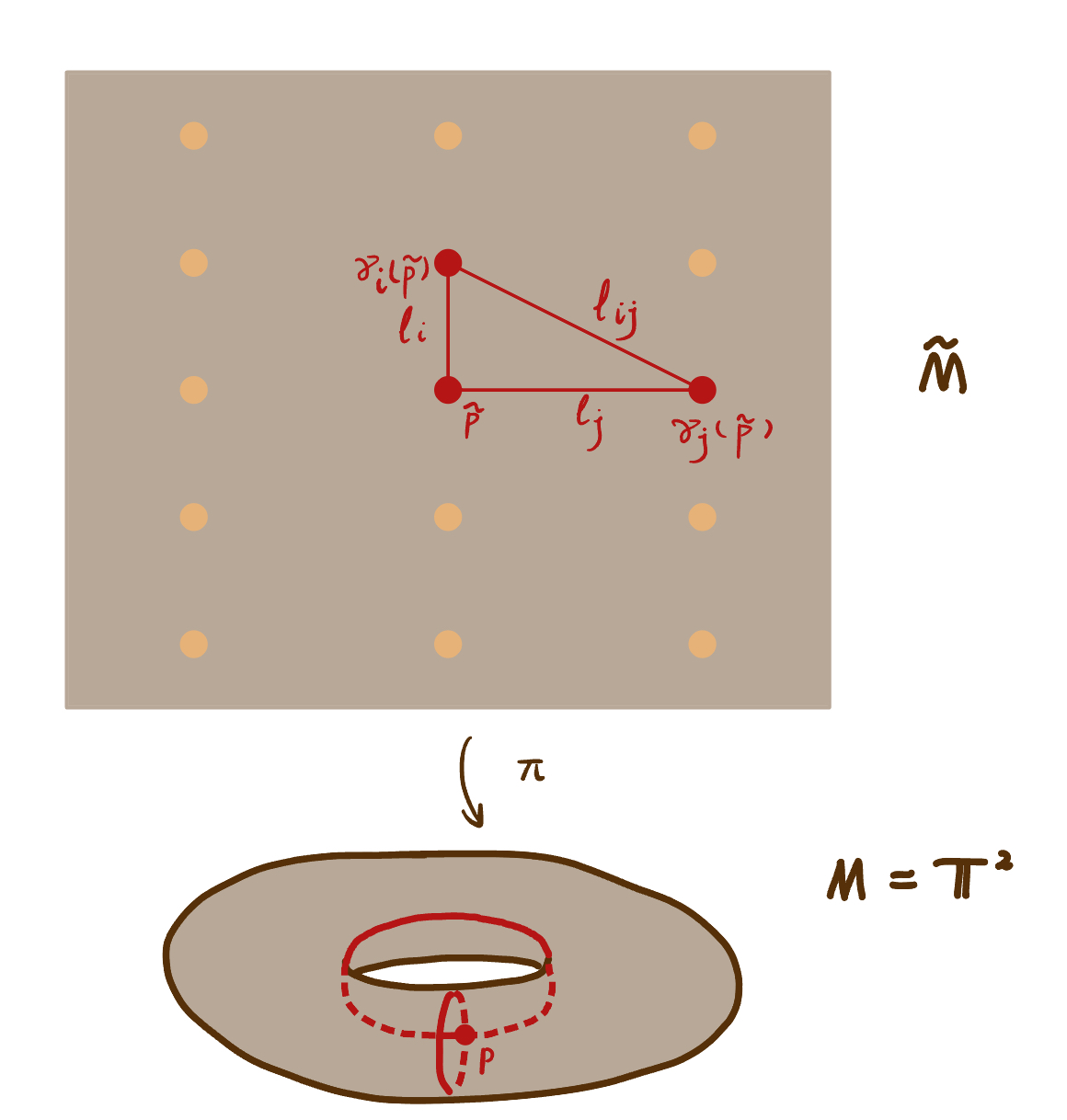
By assumption, since is a connected Riemannian manifold, we know the universal cover and the projection map exist. As a universal cover, must be simply connected, which means we have the following isomorphism between the deck transformation group (automorphism group) and the fundamental group
This isomorphism identifies each with an unique deck transformation , i.e. is an homeomorphism acting on the universal cover such that . Thus, we can say the fundamental group acting on the universal cover and for each , we denote by .
We would like to recall that the fundamental group action on the universal cover admits many good properties. Denote ,
-
•
acts freely on , i.e. for any , if for some , then must be the identity element in ; This just the property of Deck transformation on any covering space.
-
•
acts transitively on each fiber with , i.e. for any , there exists a such that ; This because a universal cover must be a normal cover, which acts transitively on each fiber.
-
•
acts properly discontinuously on ; Namely, for all compact subset , the set
is finite. Indeed, if this is not true. Then there is a compact set and an infinite sequence of such that . Then for each , we can find for each , which produces a sequence . Since is compact, we know that there is a sub-convergent limit . Taking a small neighborhood of , then is evenly covered by . But by the construction of , there are infinitely many so that for infinitely many . Then the set is an infinite discrete subset in . Moreover, the set must also be compact since it is a closed subset of the compact set . Then the contradiction arises as we know there is no discrete space with an infinite number of points that is compact.
-
•
acts isometrically on if we endowed with the induced metric, say from . i.e. for any ,
for any . Indeed, if we denote and the family of paths from to and the family of paths from to respectively, by the definition of deck transformation (), we have
therefore,
One can construct a short basis of at as the following. Fix a base point in such that via the projection . For each , we can define
the length of .
Remark 5.1.5.
the length of is dependent on the choice of , i.e. in general, we CAN NOT have
for any other This is because
but in general, the fundamental group is not abelian. Thus it is not necessarily true that and therefore
Take the geodesics connecting and . Since . Then is the geodesic loop at representing . Notice that (the length of the geodesic loop in metric ).
![[Uncaptioned image]](/html/2404.09792/assets/comparison_images/lec6image/IMG_2121.jpg)
Now we want to construct a sequence of geodesic loops at via the following procedure:
| Take to be a shortest in . Denote | ||
| Take to be a shortest in . Denote | ||
| Take to be a shortest in where | ||
The sequence is called a short basis of at .
Lemma 5.1.6.
Let be compact. Then each of its short basis has the length .
Proof.
We should prove this lemma by induction. The base case is to show . Suppose not, i.e. , after writing in terms of the generators of the fundamental group
given by Lemma 5.1.4, for each . This implies , which is impossible since is shortest in .
Now, assume all have length no bigger than . And we want to show . Suppose not, i.e. . We can again write in terms of its generators
We know one of its generators belongs to . By Lemma 5.1.4, the length of the generator must be less than . Thus we have
This contradicts the fact that is the shortest in . ∎

Remark 5.1.7.
By construction
but in general, these inequalities need not be strict, i.e. it is possible that for some . For example, the two generators of the fundamental group of a square torus might have the same length.
We would like to mention that while a short basis at is not unique, its length spectrum is unique. Denote the subgroup of generated by all loops of length at most . And define
the subgroup generated by the short basis of length at most . Since the subgroups are invariantly defined and do not depend on the choice of a short basis, the uniqueness on the length spectrum easily follows the following proposition
Proposition 5.1.8.
for any .
Proof.
It is obvious that since each .
Now we want to show the converse inclusion. Pick the largest such that . Then belong to but does not. By construction is a shortest element of outside of . Moreover, consider any other , we find
Let , then by definition
and for each . Suppose for contradiction that . This means at least one of . Thus our previous discussion,
On the other hand by above . This is a contradiction and hence . ∎
Proof of Theorem 5.1.1..
Since is complete, we have a possibly infinite sequence of loops
which forms a short basis of at . Suppose , consider the triangle , we denote
We claim that . The second inequality is trivial. Let us show that . It is also easy to check that . To see this, we only need to show . Because acts on by isometries, i.e. or any , , , we have
Then assume , that is . Since , then , When choosing the ’s elements of the shortest basis from , we need to take instead of , which gives us the contradiction.
Consider the case when . By Toponogov’s angle comparison 3.3.2, since is the longest side of this triangle, we have by the cosine law. To see why, we firstly notice that
And by Toponogov’s angle comparison 3.3.2, we have . We draw the initial vectors for each . This tells us the angles between any of these vectors . (See the following picture)
![[Uncaptioned image]](/html/2404.09792/assets/comparison_images/lec6image/IMG_2124.jpg)
Look at balls of radius in around , they are disjoint, i.e. .
![[Uncaptioned image]](/html/2404.09792/assets/comparison_images/lec6image/IMG_2125.jpg)
Since where is the number of the balls. We know that
| (5.1) |
which is the second part of Gromov’s theorem. Notice that is the number of the elements in the short basis of in the special case when .
Now, we consider the general case of , , but (The case has been done in the above.). By rescaling, we only need to consider the case when .
For general lower curvature bound , we conclude that . Following the same procedure, the balls are disjoint in . These vectors with pairwise angles . Then, we can conclude that
| (5.2) |
∎
Remark 5.1.9.
Notice is finitely generated if there is such that . This is always the case for compact manifolds as Gromov’s theorem implies since every compact Riemannian manifold has a finite diameter and satisfies some lower curvature bound (If is compact then this is a such that 111This is not a geometric argument at all. The infimum of a continuous function over a compact set can always be attained.). It can also be seen in a more elementary way as follows. Recall that if is compact and , then is generated by loops of length . And hence , i.e. all has length at most by Lemma 5.1.4. In other words, in the construction of , we only consider the loop of length . Since is compact, then there are only finitely many elements of such that . Thus we have a finite short basis. However, if is not compact then a short basis need not be finite.
Corollary 5.1.10.
. If admits , . This is because
| number of generators of |
Later, Gromov proved that the higher Betti numbers are also bounded by .
5.2 Grove-Shiohama Sphere theorem
5.2.1 Topological Rigidity Problem of Curvature Bound
The study of controlling the topology of a manifold via the Riemannian structure (curvature) of a Riemannian manifold has a long history.
Here is a trivial example followed by the Gauss-Bonnet theorem. A 2-dimensional orientable compact and simply connected Riemannian manifold with positive sectional curvature (positive Gauss curvature) must be homeomorphic to a -sphere. Indeed,
Since is simply connected, it must be orientable as well. Therefore, must be homeomorphic to by the classification theorem.
Remark 5.2.1.
Hamilton [Ham82] proved that any closed -dimensional simply connected Riemannian manifold with positive sectional curvature must also be diffeomorphic to . The Ricci flow method was first introduced in this paper. In fact, what is proved is a stronger argument: Any closed -manifold that admits strictly positive Ricci curvature and also admits a metric of constant curvature. As a corollary: Any simply connected closed -manifold that admits a metric of strictly positive Ricci curvature is diffeomorphic to the -sphere.
As for higher dimension, one result that we have studied is Myer’s theorem 4.3.1: For Riemannian manifold , if implies the Riemannian manifold compact, in particular, . By rescaling the Riemannian metric, we have
Since this also applies to the universal cover it follows that is compact and hence is finite.
Next, the following sphere theorem, which characterized the topology of the bounded sectional curvature manifold more precisely, was posed by Rauch [Rau51] and later resolved by Berger [Ber60] and Klingberg [Kli61].
Theorem 5.2.2 (The Quarter Pinched Sphere Theorem).
If is a complete, simply connected, Riemannian manifold with , then .
Remark 5.2.3.
Remark 5.2.4.
If we replace the assumption by , the classical sphere theorem 5.2.2 fails. Here is a counter-example (See Exercise 12, Chap. 8 in [dC92]): The sectional curvature of complex projective space , lies in the interval but is not homeomorphic to a sphere. In fact, it was proved by Berger [Ber60], that if , then either
-
•
and , or
-
•
and is isometric to a rank symmetric space (See [CE75])
In this section, we are going to study, in detail, the sphere theorem due to Grove and Shiohama [GS77], in which they replacing the upper bound of the sectional curvature with a lower diameter bound.
Theorem 5.2.5 (Grove-Shiohama Sphere Theorem).
If is a complete Riemannian manifold with and , then .
Remark 5.2.6.
In 1993, Grove and Peterson [GP93] generalized Theorem 5.2.5 to Alexandrov spaces, which is going to be introduced in Chapter 13 of this lecture notes. In this generality to get a sphere theorem one needs to replace the diameter lower bound with a stronger assumption of a lower radius bound. Given a metric space , the radius is defined by
It’s easy to see that . Therefore, the assumption on is stronger than . Grove and Petersen proved that if is an n-dimensional Alexandrov space of and , then is homeomorphic to .
Remark 5.2.7.
For further developments on topological sphere theorem and differential sphere theorem, see surveys by Wilking [Wi07B], Brendle and Schoen [BS09].
Remark 5.2.8.
The lower diameter bound , given in the assumption of Grove-Shiohama theorem 5.2.5 is sharp. For examples, , and has and but they are not homeomorphic to . The work of Gromoll-Grove-Wilking [Gro87, Wi07A] fully classify the rigidity of the manifolds when . That is, if is a compact manifold with and , then either or it is isometric to one of , , and .
5.2.2 The Critical Points Theory of the Distance Function
Our goal in this section is to prove the Grove-Shiohama sphere theorem 5.2.5. The key is the critical point theory of the distance function [GS77, Gro93].
Remark 5.2.9.
The critical points theory is also called the Morse theory of distance functions. In the Morse theory, one relates the topology of a Riemannian manifold to the critical points of a Morse function on .
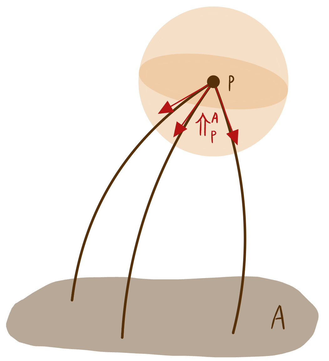
Let be a complete manifold, a closed subset. Let the distance function to . Given a , , We denote the family of unit initial vectors of the distance minimizing geodesics from to by . To clarify consists of directions of shortest geodesics such that and .
Firstly, we are going to introduce the first variation formula.
Theorem 5.2.10 (First Variation Formula).
Given with , a closed subset, , as above. Let be a unit vector at . Then exists and
| (5.3) |
where is the smallest angle between and the shortest geodesic from to , i.e. . The equation 5.3 is called the first variation formula of along .
Proof of the First Variation Formula 5.2.10.
The distance function is semi-concave on . Hence, the function as the infimum of the distance functions over , must also be semi-concave. Hence the directional derivative exists.
For simplicity, assume . Denote the unit speed geodesic starting at in the direction by . is the minimum angle between and the initial vector of the geodesics starting at to . We denote and . (see the following picture).
![[Uncaptioned image]](/html/2404.09792/assets/comparison_images/lec6image/IMG_2138.jpg)
And by the hinge comparison
Then by the cosine law
which can be differentiated at . That is
Therefore, we can conclude that , where a constant depends on . Thus
for near , more precisely for some . We can make more precise. Recall that . Let , then
This estimate follows the hinge version of Toponogov which gives that for all small .
![[Uncaptioned image]](/html/2404.09792/assets/comparison_images/lec6image/IMG_2230.jpg)
Next, we are going to show so that we can conclude thet . Let and look at where is the angle between and the shortest geodesic from to . Then where is some shortest geodesic from to . And . Note that by the definition of , we have that . By the same argument as above,
Therefore . Then taking we conclude that . Since this implies that . ∎
Definition 5.2.11 (Regular/Singular Points).
Let be complete. Let be a closed subset. Let be given by .
Now we want to give the definition of the critical points of the distance function. A point is called a regular point of if there exists such that . If no such point vector exists, then is called a singular or critical point of .
is a regular value of if the level set is a set of regular points. Otherwise, is a singular/critical value.
Remark 5.2.12.
This definition for singular and regular points can also be applied to general semi-concave functions.
Remark 5.2.13.
If a point is a regular point of , by the first variation formula, we know that there exists a unit , . That means for any . If is singular, then for any unit , we can always find a vector such that the angle between and is less than or equal to .
![[Uncaptioned image]](/html/2404.09792/assets/comparison_images/lec7image/IMG_2127.jpg)
Example 5.2.14.
Consider . Let . Then all points of except for are regular.
![[Uncaptioned image]](/html/2404.09792/assets/comparison_images/lec7image/IMG_2129.jpg)
Note that must be regular outside of the cut locus of a point . But this example shows that it can also be regular at some points of cut locus.
Example 5.2.15.
If consists of only a single vector corresponding to the unique shortest geodesic from to then is regular. This is because we can take so that by the first variation formula, we have .
![[Uncaptioned image]](/html/2404.09792/assets/comparison_images/lec7image/IMG_2130.jpg)
Example 5.2.16.
Consider .
![[Uncaptioned image]](/html/2404.09792/assets/comparison_images/lec6image/IMG_2133.jpg)
Let is the center of the square, on . Then, are critical points. The other points are regular. This is easy to verify by drawing the following pictures.
![[Uncaptioned image]](/html/2404.09792/assets/comparison_images/lec6image/IMG_2134.jpg)
Definition 5.2.17.
Let be complete, a closed subset. Denote and consider an open subset such that is regular on . A -vector field on is called gradient-like for if for any .
Proposition 5.2.18.
Let be regular on an open subset . Then there exists a smooth gradient-like vector field for on .
Proof.
Firstly, we want to prove the gradient-like vector field exists locally. From the classical theory of differentiable manifold, we know that given a vector for some , we can always extend to a smooth global vector field on such that . Based on this fact, we claim that when is a regular point so that , we can find a sufficiently small neighborhood of such that the restriction of is a gradient-like vector field.
Suppose not, then we can find a sequence of points such that .
![[Uncaptioned image]](/html/2404.09792/assets/comparison_images/lec6image/IMG_2139.jpg)
And for each index , there exists shortest geodesic from to such that . Since the initial vector all lies in a unit sphere, which is certainly compact, then we can extract sub-sequences from and such that
And this implies the sub-convergence of the angles:
Also as a limit of shortest geodesic from to is the shortest geodesic from to .
Therefore, is also critical. And this is a contradiction. Therefore, we know that
Since is regular on we can do this near any point in . Hence we can cover by open sets such that each admits a gradient-like vector field .
Then we can glue them into a global vector field on using partition of unity subordinate to this cover of . And take with and on . And we know that and locally there are only finitely many of . We claim that is gradient-like for . Recall that is concave on for any ,
Moreover, the last inequality is strict since there exists such that . Note that if is gradient like for on , then is also gradient like. WLOG, we can conclude that there exists a unit gradient-like vector field. ∎
Corollary 5.2.19.
From the first part of the proof of Proposition 5.2.18, we know that if is a regular point, then we can find a sufficiently small neighborhood of such that every point is regular.
From now on, we will assume is gradient-like and .
Lemma 5.2.20.
For and being regular on open subset . Let be compact. Then there exists such that increases with speed bigger than along the integral curves of contained in , i.e. if is an integral curve of and , we have for ,
Proof.
Recall the Rademacher theorem, since is locally Lipschitz, is differentiable almost everywhere and
consider , Lipschitz, then
We claim that . Suppose not, that is (it is obvious that ). We take a minimizing sequence for . By compactness of , we can say that there exists such that up to subsequence.
![[Uncaptioned image]](/html/2404.09792/assets/comparison_images/lec6image/IMG_2140.jpg)
Since , where the shortest geodesic from to which touches at and . Then . Hence . This contradicts that is gradient-like for on .
∎
Lemma 5.2.21.
Let . Let be a regular value of thus has no critical points. Then is an -dimensional topological manifold.
Proof.
By definition, we need to show that for any , we can find a neighborhood homeomorphic, say via , to an open subset of .
By Proposition 5.2.18, we can construct a unit gradient-like vector field near . Take be a smooth submanifold transversal to near , i.e. such that .
![[Uncaptioned image]](/html/2404.09792/assets/comparison_images/lec6image/IMG_2141.jpg)
Look at a small neighborhood of . on which is regular. Notice that is compact. Then by the previous lemma 5.2.20, increases with speed along the integral curves of in . Thus, there exists such that
| (5.4) |
where is the integral flow of .
![[Uncaptioned image]](/html/2404.09792/assets/comparison_images/lec6image/IMG_2142.jpg)
Therefore, has unique intersection with , which means there exists a unique such that .
It is easy to see that is continuous since is. Here is why: If it is not continuous at some . Then
| such that | |||
However, by the uniqueness of , we know that . Therefore, is continuous. This gives us a map such that is a local homeomorphism near . Therefore, the level set is an -dimensional topological manifold. ∎
Theorem 5.2.22 (Morse Type Theorem 1).
Let be given by or more generally, is semi-concave and Lipschitz. Let , assume is compact and is regular in . Then
and
In particular,
Proof.
Take as a smooth unit speed gradient-like vector field on . Since is regular in , then there exists a constant such that for any . This means our function along the gradient curves in increases with the speed of at least . We claim that the for any , there exists a continuous function such that
![[Uncaptioned image]](/html/2404.09792/assets/comparison_images/lec7image/IMG_2131.jpg)
Firstly we can find a such that we can flow any by the gradient flow to somewhere beyond the level set , i.e . This is possible since for by the lemma 5.2.20. So we can take . Suppose , then . As , we can conclude that . Hence, there exists such that for any . And this is unique since is monotone increasing for and is continuous in by the same arguments as in the lemma 5.2.21. Now we want to construct a homeomorphism to finish our proof. The homeomorphism can be constructed as follows,
In this map, and .
We claim that is a homeomorphism. To show that is onto, for , we can flow back to some point . Thus we can find . Next, we can construct the integral curve via the flow passing through at some time .
![[Uncaptioned image]](/html/2404.09792/assets/comparison_images/lec7image/IMG_2132.jpg)
these spaces are Hausdorff and compact so it’s enough to prove that is a continuous bijection so only injectivity needs to be checked. Indeed, suppose , then it must be . Otherwise, the flow lines would not intersect all the way along and thus we will have . It is also impossible that due to the fact that is strictly monotone with respect to along the flow lines. ∎
Theorem 5.2.23 (Morse Type Theorem 2).
Using the same proof as in Theorem 5.2.22, we can also show that if is regular over , then
and
If in addition is smooth, then .
Proof.
Let us first treat the case when is smooth. Let be a smooth gradient-like vector field of on . Then must be transverse to . Let be the flow of . Then we claim that is a diffeomorphism. Since is transverse to the map is a local diffeomorphism. Hence we only need to claim that this map is bijective. The proof for being a bijection would be the same as the proof for Morse Theorem 1 5.2.22. To show is surjective, that is for such that , compact. On , since , in the finite time flowing backward, we hit at some . Therefore is surjective. Moreover, is injective by the uniqueness of .
To show the homeomorphism case, we can write
By Morse Theorem 1 5.2.22, each can be written as the produce which is homeomorphic to . By gluing these together, we have
∎
Corollary 5.2.24.
If has no critical point in . Then
where is the closed unit disk in .
Proof.
The first step is to take a sufficient small . Then
Next, by Morse Theorem 1 5.2.22, since has no critical point in . We can write the annulus as
![[Uncaptioned image]](/html/2404.09792/assets/comparison_images/lec6image/IMG_2143.jpg)
Therefore, .
∎
Lemma 5.2.25.
Let be a complete manifold, a compact subset, let . If is a regular value of , i.e. is a set of regular points. Then is a regular value for all sufficiently small .
Proof.
Suppose not, then we can construct a sequence from the compact set such that . This sequence sub-converges in and thus the limit point lies in . Here we have a contradiction, since must be a regular point and the set of regular points is open by Corollary 5.2.19. ∎
Remark 5.2.26.
Lemma 5.2.25 might not hold if is not compact. One can construct a counterexample when the radius of the regular neighborhoods for each point of asymptotically vanishes.
Definition 5.2.27 (Compact Type).
A manifold is said to be of compact type if it is homeomorphic to the interior of a compact manifold with a boundary.
Proposition 5.2.28.
Let be an open complete manifold. Let where is a compact subset in . Let be a regular value of . Suppose that has no critical point outside of . Then has a compact type. In fact . Notice that is a compact manifold with a boundary in this case.
Proof.
Consider the embedded topological submanifold where . By Lemma 5.2.25, for some small has no critical point in , which is compact since it’s a closed subset of which is compact.
Remark 5.2.29.
Moreover, it follows from the above proof that is homotopically equivalent to and thus homotopically equivalent to , which is a compact manifold with boundary.
5.2.3 Proof of Grove-Shiohama Sphere Theorem
Denote . Let be the points such that . Denote . Since we assume , we consider the model space . For , the function satisfies
For , . As a consequence, we know that is concave in . Then by the point-on-a-side comparison 3.4.4 and the Jensen’s inequalities 3.4.12, is concave outside of .
Step 1:
We claim that has a unique maximum at .
When , then the uniqueness of the maximum follows since the perimeter of any triangle in is at most . For instance, consider such that , then the length of the side must be zero, which implies and must be equal.
Suppose and there are two distinct maximal points such that . We draw the mid-point of the segment . From the following picture, we can conclude that since is strictly concave along non-radial geodesics. Therefore, which contradicts to the fact that .
![[Uncaptioned image]](/html/2404.09792/assets/comparison_images/lec6image/IMG_2144.jpg)
Step 2: Next, we claim that has no critical point outside and . Suppose not, then there exists that is critical for . Denote be any shortest geodesic from to and be any shortest geodesic from to .
![[Uncaptioned image]](/html/2404.09792/assets/comparison_images/lec6image/IMG_2145.jpg)
We claim that the angle , in the picture, is bigger that . We want to show by cases. The first case is that when , where is a geodesic outside of .
![[Uncaptioned image]](/html/2404.09792/assets/comparison_images/lec6image/IMG_2146.jpg)
In this case, is concave. And because , we have .444Otherwise, if , because concave function is below the tangent line, for all , thus . Contradiction. By the first variation formula, . On the other hand, we apply the same argument to to prove the case when and conclude . In the last case where and , apply the hinge comparison, we have . However, in the model space , since both , we can conclude that . By the cosine law, since , we have
Then the contradiction arises since but . Therefore, in any cases, we have , which implies is not critical for (and also for ).
Step 3: Consider small -neighborhoods of and . Construct gradient-like unit vector field for on , which is radial for on . On . by Step 3 we can take . By Lemma 5.2.20 on . On , and is compact. We claim that is homeomorphic to . For any , we can extend the integral curve through backward and forward, it hits both and exactly once. This is because it will eventually hit both and . Thus we will have to intersect both and . It is impossible for us to intersect and more than once since the vector field is transversal to both of the surfaces which separate the manifold into two components. Thus there exists a unique such that . As before, is continuous. Now, we construct
We can easily see that is onto. And is continuous since is continuous and is continuous. To show is one-to-one, i.e. and . Suppose , then flow lines through do not intersect, which is impossible. On the other hand, since , then Therefore, is a homeomorphism.
Step 4: Now we are going to finish our proof. Since is a homeomorphism,
Because so that is a twisted sphere, i.e. where is an homeomorphism as well. We need to introduce the following lemma
Lemma 5.2.31 (Alexander’s Trick).
Any homeomorphism can be extended to a homeomorphism between disks by the formula
Corollary 5.2.32.
Any twisted sphere is homeomorphic to a sphere.
By Alexander’s trick, we can extend and get the homeomorphism from to . By the following picture, we denote the upper and lower halves of .
![[Uncaptioned image]](/html/2404.09792/assets/comparison_images/lec6image/IMG_2147.jpg)
And we map to . And we glue the image via the homeomorphism . Finally, we apply the Alexandrov trick to extend the upper sphere so that we construct the homeomorphism for to .
Remark 5.2.33.
What if is a smooth twisted sphere and is a diffeomorphism. Is still diffeomorphic to ? Notice that our proof using the extension of no longer works. Since the extension is not smooth at the center of the ball. However, in 1956. Milnor proved the following theorem.
Theorem 5.2.34 (Milnor [Mil56]).
There exists a exotic twisted 7-sphere, that is there exists exists diffeomorphism such that . However, is not diffeomorphic to . Therefore, is an exotic sphere.
Open Question 5.2.35.
If admits and , then is diffeomorphic to .
By 6.2.8 there exists an exotic sphere which admits a metric of .
Open Question 5.2.36.
Does there exist an exotic sphere that admits a metric of ?
Chapter 6 Manifolds of Nonnegative Curvature
Example 6.0.1.
For . we have and . For . we have , , .
Let be a compact Lie group with a bi-invariant metric
Definition 6.0.2 (Left(Right) Invariant Metric).
Let be a compact Lie group. Then
-
•
is called left invariant metric if ;
-
•
is called a right invariant metric if
for all and . is called a bi-invariant metric if it is both left and right invariant.
Fact 6.0.3.
If is a Lie group with a bi-invariant metric, then . Every compact Lie group has a bi-invariant metric.
For example, .
We denote the set of unitary quaternion matrices. In particular, is a compact Lie group. Here denotes the division ring of quaternions.
And
We know that and have nonnegative curvature with respect to the canonical bi-invariant metric (See Remark 6.0.4).
Remark 6.0.4.
We would like to explain what we mean by canonical metric here. We denote where the space of matrixes with and entries. The metric for these spaces are defined as
where is the Hermitian transpose (conjugate transpose) so that in the case of , . Notice, that the above metric is just the Euclidean metric if we consider an -matrix as a vector with -entries. Thus, one can induce the metric of , and canonically using the above metric.
6.1 Review: Riemannian Submersion
Definition 6.1.1 (Riemannian Submersion).
Let be a smooth submersion (). For each , we can decompose into two components:
-
•
The vertical tangent space at is ;
-
•
The horizontal tangent space at is .
Since is a submersion, is an isomorphism.
Then is a Riemannian submersion if and only if for any , the isomorphism is an isometry, i.e.
for any
Remark 6.1.2.
At each , we have an orthogonal decomposition for as a direct sum .
Remark 6.1.3.
By the submersion level set theorem, at each , each fiber is an embedded smooth submanifold of . Thus we can also write .
Proposition 6.1.4.
A Riemannian submersion is -Lipschitz.
Proof.
We want to show for any pairs of . Let be any curve connects and , then
By taking the infimum among all such it follows that is -Lipschitz. ∎
Here we introduce some important examples of Riemannian submersions.
Example 6.1.5.
Let be a Lie group that acts freely, isometrically and with closed orbits on . Then inherits a natural Riemannian metric such that is a Riemannian submersion.
Example 6.1.6 (Warpped products).
Suppose and are Riemannian manifolds. Let be smooth, then the projection is a Riemannian submersion.
Definition 6.1.7 (Horizontal Lift).
Let be a smooth submersion, a vector field is a horizontal vector field (resp. vertical vector field) if for each , (resp. ).
Given , a vector field is called a horizontal lift of if for each ,
In particular, for each , let be a curve starting at . A curve starting at some is called a horizontal lift of if for each , and
Notation 6.1.8.
We denote the family of smooth vertical vector fields of and the family of smooth horizontal vector fields of .
The following is the principal property of horizontal vector fields
Proposition 6.1.9 (See Proposition 2.25 in [Lee19]).
Let be a smooth submersion between two Riemannian manifolds. Then
-
1.
Every can be uniquely expressed in the form where and ;
-
2.
Every has a unique smooth horizontal lift to ;
-
3.
For every and , there is a vector field whose horizontal lift satisfies .
Proposition 6.1.10.
Let be a Riemannian submersion between two Riemannian manifolds. Fix , then for each regular curve starting at , there is a unique regular horizontal lift starting at .
Proof.
Since the regular curve is a locally embedding. WLOG, we only need to consider the case that is a smooth embedding and has no self-intersection, since otherwise we just split into many small pieces. Consider the vector field , we can have a global extension of this vector field over . And then by 2. in the proposition 6.1.9, we have a unique horizontal lift of , say over . Then by taking the integral curve of , we can we have a unique smooth horizontal lift of . And we just take be the integral curve of the smooth horizontal lift of starting at . The uniqueness follows by the uniqueness of integral curves. ∎
By construction, an important observation is that
In particular, if is a shortest geodesic from to , then the horizontal lift is a shortest geodesic as well. Indeed. Let be the endpoint of . Then
Thus, all the inequalities above are equalities, and hence is length minimizing between its endpoints. Therefore, we can conclude the following corollary.
Corollary 6.1.11.
Every horizontal lift of a shortest geodesic by a Riemannian submersion is also a shortest geodesic.
6.2 Comparison Theory for Riemannian Submersions
Theorem 6.2.1.
If and is a Riemannian submersion, then as well.
Proof.
We only need to use a four-point condition to check that satisfies . That is, for , we want to show
Since is a Riemannian submersion, by the previous discussions on the horizontal lift of the shortest geodesics, given the initial point we can find such that
By assumption, , thus we have
We claim that
Once we prove that, the four-point comparison in holds, and the result follows. The key observation now is that is -Lipschitz and we should use hinge comparison, thus
Then we immediately conclude that . ∎
Remark 6.2.2.
There is another method can be found in [Bes07] using O’Neil’s formula.
We are going to list some applications of theorem 6.2.1.
Corollary 6.2.3 (See Corollary 2.29 in [Lee19]).
Fact 6.2.4.
Suppose is a Lie group with a bi-invariant Riemannian metric. Then for any it holds that (See exercise 1 page 103 in [dC92]). In particular, .
Example 6.2.5.
Example 6.2.6 (Bi-quotients).
Still let be a Lie group and let be a closed subgroup. Then such that for ,
This action is called a bi-quotient action. In a special case when belongs to either or this is a homogeneous space action. Unlike homogeneous space actions, bi-quotient actions need not be free in general.
If is compact then the bi-quotient action is proper. If the bi-quotient action of on is also free then the quotient space of the action above is a smooth manifold.
Suppose admits a bi-invariant metric (note that such a metric always exists if is compact). Then by above and by theorem 6.2.1,
| is a Riemannian submersion | |||
| will have |
Remark 6.2.7.
In the special case of where and the action of on is given by the formula
where .
Example 6.2.8.
And consider a biquotient action given by
where . It is not hard to check this action is free. Notice that . Take . Then by [GM74], is an exotic sphere of . That means but not diffeomorphic. An open question related to that is whether there exists an exotic sphere of .
Chapter 7 Cheeger-Gromoll Soul Theorem
7.1 Introduction to the Soul Theorem
The soul theorem describes the topological structure of open manifolds of non-negative sectional curvature. By open manifolds we mean non-compact complete manifolds without boundary.
Theorem 7.1.1 (Cheeger-Gromoll Soul Theorem).
Let be a Riemannian manifold of and it is complete and non-compact. Then there exists a closed totally convex subset which is also a totally geodesic submanifold such that
where is the total space of the normal bundle of . In particular, has compact type (See Definition 5.2.27) since
where the unit disk bundle of is also a compact manifold with a boundary.
There are some suggestive examples to explain the theorem. Given a Riemannian manifold with . Then . Suppose be a closed subgroup such that by isometries freely. Also by matrix multiplication. We can take the diagonal action of on , i.e. . Then by 6.2.3.
Consider the following vector bundle.
We can conclude that both the total space and the base of this bundle are manifolds of non-negative sectional curvature and the projection map is a Riemannian submersion. Note that the total space is necessarily non-compact and the base is compact if and only if is.
The following two examples are special cases of the above construction.
Example 7.1.2.
, . We equip with the canonical bi-invariant metric.
We know that by
Then on the left. This action is obviously free and isometric. Consider the vector bundle
Fact 7.1.3.
We want to show this vector bundle is the tangent bundle to in any dimension and admits a metric of complete Riemannian manifold of .
Example 7.1.4.
Consider , . acts on by
Also, acts on the unit sphere by the formula above. We take the bundle
This is the Hopf bundle and by above it admits a metric of nonnegative sectional curvature.
7.2 Busemann Functions
Definition 7.2.1 (Ray).
A globally distance minimizing unit speed geodesic is called a ray i.e.
Lemma 7.2.2.
If is complete and non-compact, then contains a ray starting at any point .
Proof.
By non-compactness of there is a sequence such that . Connect using a shortest geodesic , denote the unit vector in . By compactness of , we can find a such that upto subsequence. Thus
Claim 7.2.3.
is a ray. Fix , then . So
| is a ray. |
∎
Definition 7.2.4 (Busemann Function).
Let be a ray, . Then a Busemann function for is defined as
Claim 7.2.5.
We claim that a Busemann function is always well-defined and finite.
Proof.
Since , by the triangular inequality we have
This means that the quantity is bounded.
Let , then
Therefore, is always non-increasing and bounded. Thus, it has a limit as . Therefore, is always defined and finite. ∎
Property 7.2.6.
is -Lipschtiz.
Proof.
For each , let , by the triangule inequality we have
Therefore we can conclude that the Busemann function is always 1-Lipschitz as a limit of 1-Lipschitz functions. ∎
Property 7.2.7.
For any , .
Proof.
By direct substitution, for each , we have
∎
Example 7.2.8.
We are going to give a qualitative example to strengthen our intuition on the sub-level set and the super-level set of the Busemann function. We draw the following picture, Let be a paraboloid in and let be a point. Consider a ray starting at and going upwards.
![[Uncaptioned image]](/html/2404.09792/assets/comparison_images/lec7image/IMG_2162.jpg)
By the previous property 7.2.7, we know that for any . Because the Busemann function is -Lipschitz, then for any , take the shortest geodesic from to , which intersect at some , then we know that
If , any point near , . This is because
On the other hand, we can extend in the opposite direction. It will remain globally shortest until it hits the apex of the parabola. Then
If we pick some before the geodesic hits the apex, we can still take some near . In this case,
Property 7.2.9.
Given any point, For a sequence , denote the initial vector of starting at . Then by compactness sub-converges. We claim that
| (7.1) |
That is along , decreases with unit speed.
Proof.
Fix , , denote for each .
![[Uncaptioned image]](/html/2404.09792/assets/comparison_images/lec6image/IMG_2149.jpg)
Since the unit initial vectors sub-converge to , and , sub-converges as well. Then
∎
Moreover, the equation 7.1 also implies that is a ray, i.e. for any . We can show this by contradiction. Suppose not, . Since is -Lipschitz, then . However, it is known that .
Lemma 7.2.10.
For , .
![[Uncaptioned image]](/html/2404.09792/assets/comparison_images/lec6image/IMG_2150.jpg)
Proof.
Let , we want to show , this follows by the triangular inequality:
∎
Proposition 7.2.11.
Proof.
Let , then for some , which means . And since is -Lipschitz, we know that
Therefore, ,
The opposite direction is trivial, let , then we know that for sufficiently large . ∎
Remark 7.2.12.
For any , we have
![[Uncaptioned image]](/html/2404.09792/assets/comparison_images/lec7image/IMG_2165.jpg)
Property 7.2.13.
If , then is concave for any ray .
Proof.
In , take , . We can claim that the Busemann function is a linear function. Let us verify this for the case i.e (the general case is similar). Notice that
And since
Taking , we have
The general case is by a similar computation. We can conclude that the Busemann function in is affine, then concave as well.
Now we want to use the Toponogov theorem to show is concave in with .
As the following picture shows, fix some point , by triangular inequality . Take sufficiently small, for any , by the triangular inequality again, after fixing any , we can find a sufficiently large such that
![[Uncaptioned image]](/html/2404.09792/assets/comparison_images/lec7image/IMG_2272.jpg)
That means for large . We claim that this implies that is -concave outside of . This is because if we have and , by the Hessian comparison theorem 2.5.1 (in particular inequality 2.16), we know that
where is the orthogonal projection onto the tangent space of the sphere centered at of radius . Since for all large , we can conclude that is -concave on for all large . Therefore,
is also -concave on for all large .
By the definition of the Busemann function, we know that
is also -concave on for all . Therefore, is concave on . Since is concave near and concavity is a local property, we conclude that is globally concave. ∎
Remark 7.2.14.
There is a corresponding statement about Busemann functions on spaces of nonpositive curvature. Namely, if is complete, simply connected, and has then for any ray its Busemann function is convex.
Definition 7.2.15 (Total Busemann Function).
Let be a noncompact, complete Riemannian manifold without boundary and . Let , we can define the total Busemann function as
for each .
Remark 7.2.16.
Since a limit of rays is a ray it easily follows that this infimum is always achieved, i.e.
for any .
Definition 7.2.17 (Negative Gradient Ray).
Given a 1-Lipschitz function a ray is called a negative gradient ray for if
Note that if is a negative gradient ray for then decreases along with maximal possible speed (=1). This justifies the term "negative gradient ray".
Proposition 7.2.18.
Both and have the property that for any each of them admits a negative gradient ray starting at .
Proof.
The result for follows by Property 7.2.9.
Let and let us prove that has a negative gradient ray starting at .
By Remark 7.2.16, we know that there exists a ray starting at such that . By the Property 7.2.9, we can construct a ray starting at such that for any . Now we want to show this implies , i.e that is a negative gradient ray for starting at . Take any other ray starting at , then
since is -Lipschitz. This means
Remember that . Therefore, we can conclude that for any ray starting at ,
this means the minimum is achieved when . is a negative gradient ray for and hence . ∎
Definition 7.2.19 (Totally Convex Subsets).
A subset is called totally convex if for any and any geodesic (not necessarily shortest ) from to , it holds that .
Proposition 7.2.20.
Suppose is a total Busemann function and let , the set
is compact and totally convex. The total convexity tells us that for any , the geodesics (not necessarily shortest) connecting and lies in .
Proof.
Firstly, we claim that is totally convex. Let , and any geodesic segment connecting and such that and , because is concave,
This means , thus is totally convex.
Next, we show the set is compact by contradiction. It’s enough to prove the statement for . Note that and hence for any the set is nonempty. Suppose the set is non-compact. Then there exists a sequence such that . Because is convex, for every . By the previous argument, by taking the unit initial vector of , which sub-converge in a sphere, the segments also sub-converge to a ray starting at , saying . And . However for large and . Therefore, , which brings us to a contradiction. ∎
Notation 7.2.21.
By the compactness of Proposition 7.2.20, we know that attains the maximum on for each real number. We denote the maximum value and the maximum level set.
Proposition 7.2.22.
For , . Then
Therefore, in particular,
Thus for .
Proof.
Step 1 (Show ): Suppose this is false, there exists such that , then for some , . Since the total Busemann function is -Lipschitz, we have
This means . Contradiction.
Step 2 (Show ): Suppose this is false, then there exists such that and . In fact, we should keep in mind that
Let be a negative gradient ray of starting at such that . Then, on the other hand, (remember ). Therefore, by the intermediate value theorem, there exists such that . This means . By our assumption, we have . However, by the definition of ray, . Contradiction. ∎
Proposition 7.2.23.
has an empty interior.
Proof.
If , then we can take an interior point so that . Take and . By Proposition 7.2.22, i.e. . This contradicts the maximality of . Therefore, the set has an empty interior. ∎
Remark 7.2.24.
The set having an empty interior doesn’t mean the set must be a point.
![[Uncaptioned image]](/html/2404.09792/assets/comparison_images/lec7image/IMG_2166.jpg)
7.2.1 A Brief Plan on the Proof of the Soul Theorem
The reason why we need to introduce the total Busemann function is that the construction of the set is the key construction in the proof of the Soul theorem. To see this let’s briefly discuss our plan for proving the theorem.
We denote by , which is a totally convex subset (By Proposition 7.2.20). Considering the function , notice that is concave on (We need to check this concavity later) so that attains the maximum. Then we can take to be the maximum level set of . Take , …… We will repeat this construction as long as has a boundary.
Then we obtain a sequence of such that
and
Since the dimensions are strictly decreasing, we eventually will get a such that . Which is indeed the Soul of the manifold. Then we will show that is diffeomorphic to the total space of where means the normal vector bundle of .
To carry out this process, we need to
-
•
Understand convex subsets;
-
•
Show that is concave on is is a convex subsets of of .
7.3 Convex Subsets in Riemannian Manifolds
Definition 7.3.1 (Convex Subset).
is called convex if , there exists a shortest geodesic in such that .
Definition 7.3.2 (Strongly Convex Subset).
Let , if , any shortest geodesics connecting and will be contained in , then is called strongly convex.
Example 7.3.3.
This is an example of a convex by not strongly convex subset. Consider , an upper hemisphere, then is convex but not strongly convex.
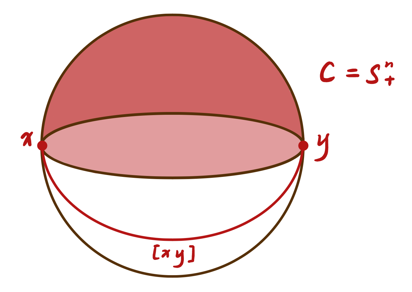
Fact 7.3.4.
Any convex subset is locally strongly convex in the following sense. For any , there exist such that is strongly convex. Thus, if is convex, then for any , there is such that is strongly convex.
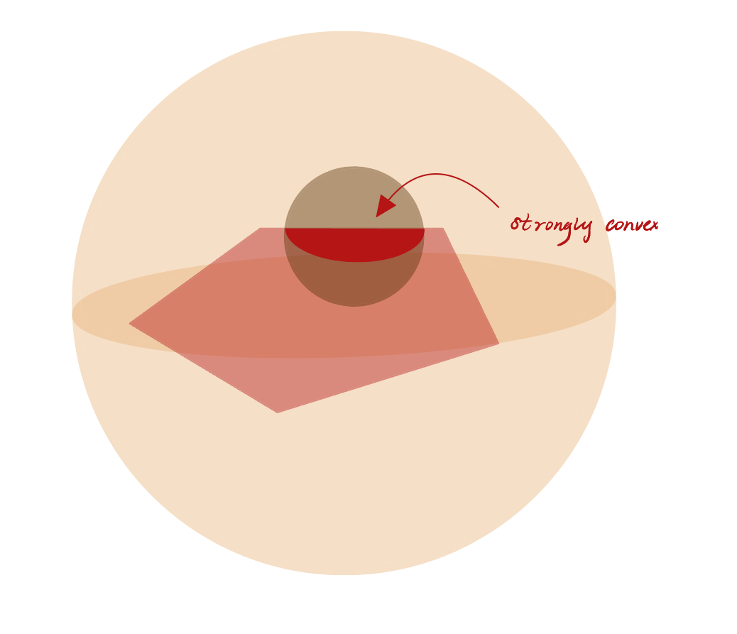
Proposition 7.3.5.
If is convex and closed, then is a manifold with boundary, and its manifold interior is convex and totally geodesic.
Proof.
Let be closed. Take as the largest possible integer such that there is a submanifold of contained in . Let , we claim that there exists such that .
![[Uncaptioned image]](/html/2404.09792/assets/comparison_images/lec7image/IMG_2168.jpg)
We prove this claim by contradiction. Suppose not. Then there exists a sequence where . We can cone off at , take near . Then is the collection of shortest geodesics. Take the union (cone)
for -small. This union will contain -dimensional submanifold of . However, we know that and this contradicts the maximality of . Therefore, for small . Therefore, is totally geodesic and locally convex. In particular is .
![[Uncaptioned image]](/html/2404.09792/assets/comparison_images/lec7image/IMG_2171.jpg)
We need the following technical Lemma.
Lemma 7.3.6.
let be convex and closed, and so that for any two points in there is a unique shortest geodesic between them and it is contained in (such always exists).
Suppose such that and . Let and let be the unique unit speed shortest geodesic with .
Then . Moreover, if then for all small .
Proof of Lemma 7.3.6.
Let be a small smooth -submanifold containing and transverse to . Such exists since . Then the punctured cone is a -manifold, it is contained in and hence it is contained in . By construction it contains .
This proves the first part of the lemma. Now suppose . If some for some small then we can repeat the cone construction with instead of and get that which is a contradiction. ∎
We are now ready to proceed with the proof of Proposition 7.3.5.
Lastly, let us show that is convex (and hence is obviously connected).
Let . Since is convex there exists a shortest unit speed geodesic such that . We claim that . If not let be the smallest such that . Then applying Lemma 7.3.6 to for a small we conclude that which is a contradiction. This proves the convexity of .
Next, let us show that is dense in . Suppose not. Then there is and a small as in Lemma 7.3.6 such that there are where and . But then the whole geodesic is contained in by Lemma 7.3.6 and therefore . This is a contradiction and hence .
It remains to show that is a topological manifold with boundary. We will only sketch the argument.
Look at , we want to show this is a dimension topological submanifold of and is relativity open in the topology of . Take , take near , take for some sufficiently small such that .
![[Uncaptioned image]](/html/2404.09792/assets/comparison_images/lec7image/IMG_2177.jpg)
Connect points near by shortest geodesics with , we can get a homeomorphism
moreover, this map has an inverse map from the neighborhood of in to . Then it is not hard to show is the well-defined and continuous inverse of each other (followed by the uniqueness of points of intersection.). Finally, we can conclude that is -dimension manifold with boundary. (This is the general result of the convex set of the Riemannian manifold.) ∎
Example 7.3.7.
Let be a closed and convex subset. Then there is an affine subspace such that is a -dimensional convex body. It’s a manifold with a boundary but the boundary need not be smooth.
Definition 7.3.8.
Let be a closed convex subset. Take , and denote
the tangent cone of at .
![[Uncaptioned image]](/html/2404.09792/assets/comparison_images/lec7image/IMG_2273.jpg)
Example 7.3.9.
Consider the above region , at , the tangent cone is a half-space. At , the tangent cone has an angle.
7.4 Concavity of the distance function
Theorem 7.4.1.
Let be a manifold with . be a closed, convex subset with boundary (as a manifold). Denote on . Then is concave on . i.e. for any geodesic , is concave.
Proof.
Fix , it is enough to prove there exists a supporting linear function that is always bigger than near . i.e. and for all near as in Figure 7.3.
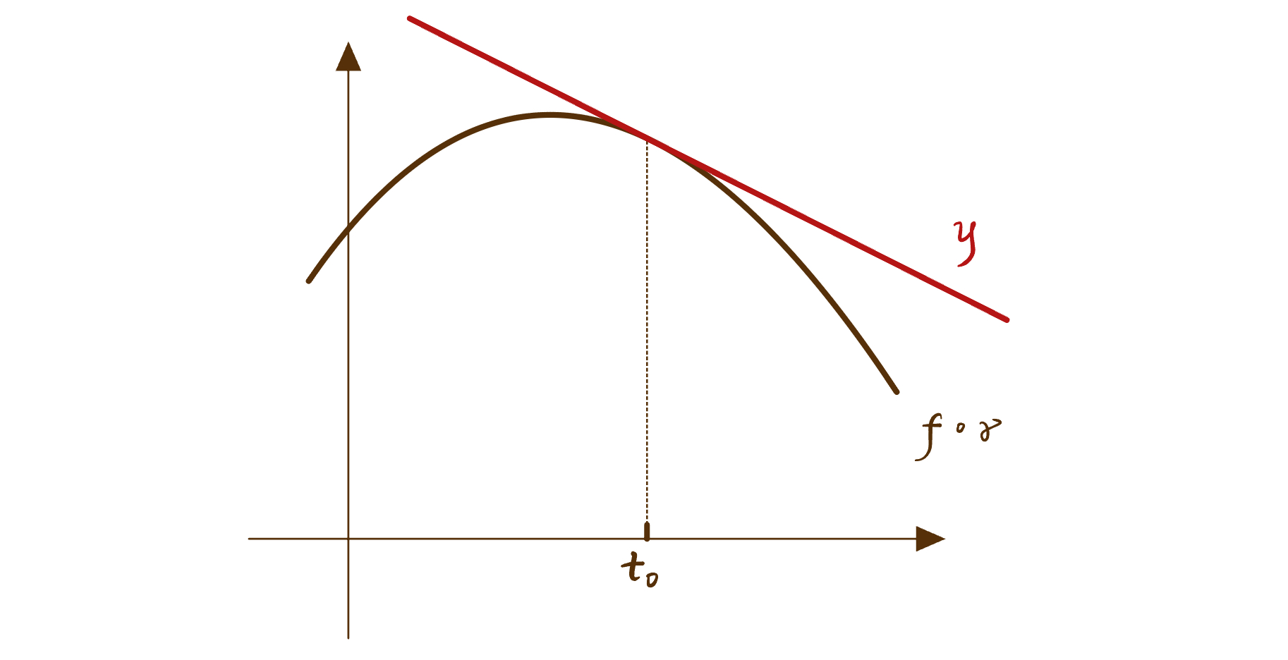
We are going to start the proof by discussing some geometrical setting. Let be the closest to on so that . Let , then we claim that the angle between and the initial vector of the geodesic segment starting at , i.e. , must be at least .
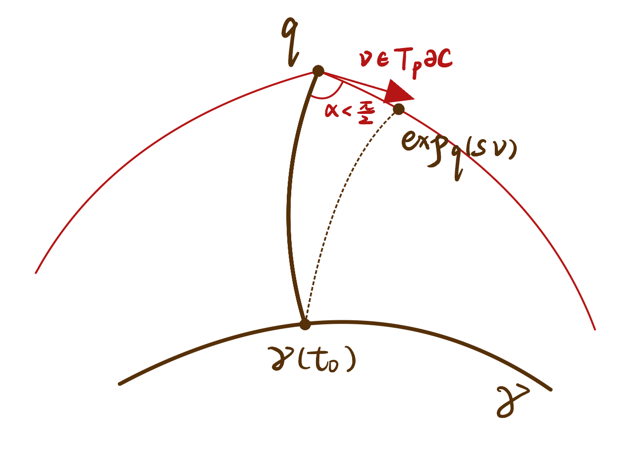
Suppose not, i.e. . Then by the first variation formula:
This means for sufficiently small , is no longer the closest point to on , i.e.
Contradiction.
Remember that is convex and the subset of some half space . Now we want to claim for the initial vector of , we mush have .
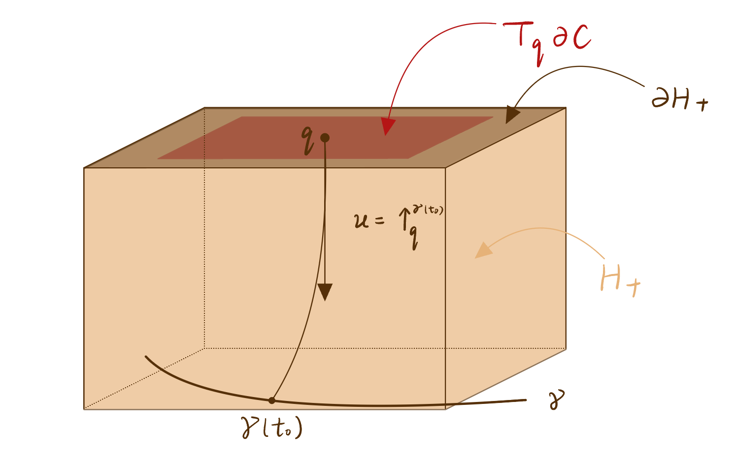
Suppose not. Then there will be direction such that
which is impossible due to our previous claim. That means . Then is unique since it must be perpendicular to . This also shows that the half-space containing is unique as well.
Next, we are going to define the supporting linear function and show that near . We parameterize the geodesic segment by a unit speed curve and consider the angle . We define the linear function as
| (7.2) |
the slope term is motivated from the first variation formula 5.2.10. Because has a derivative at , then by the first variation formula
We consider 3 cases depending on whether or .
Case 1. . Take and extend it to a parallel vector field along . Then for each . In particular, so that .
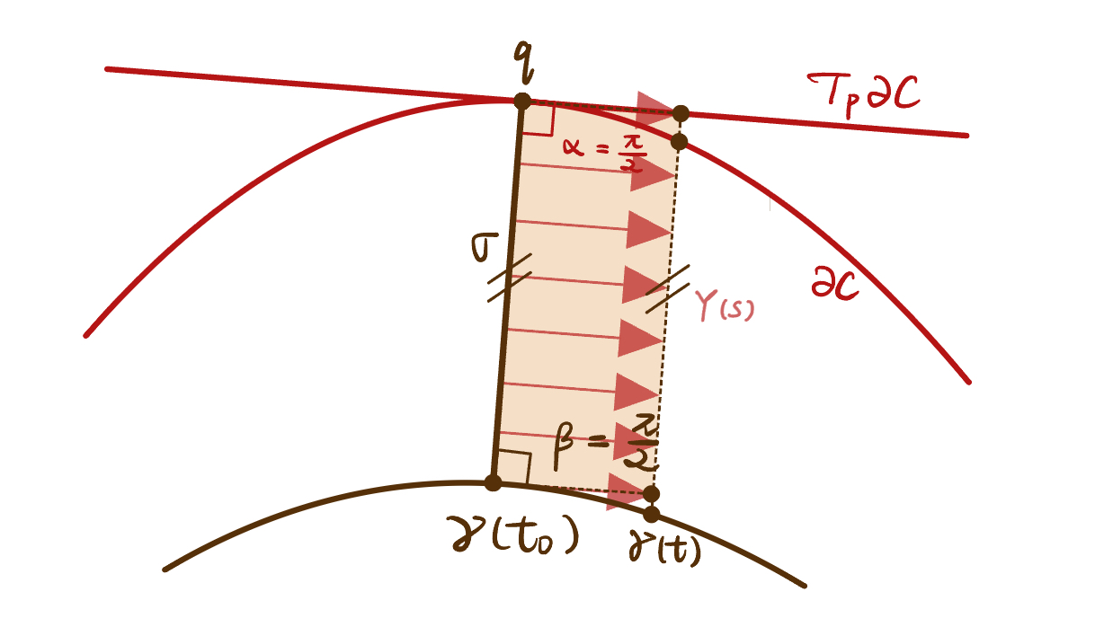
Let . We quickly got that
In the Figure 7.7 below, because is concave so that the geodesic connecting and intersect at some point say . Here we denote and the corresponding points of and in the model space.
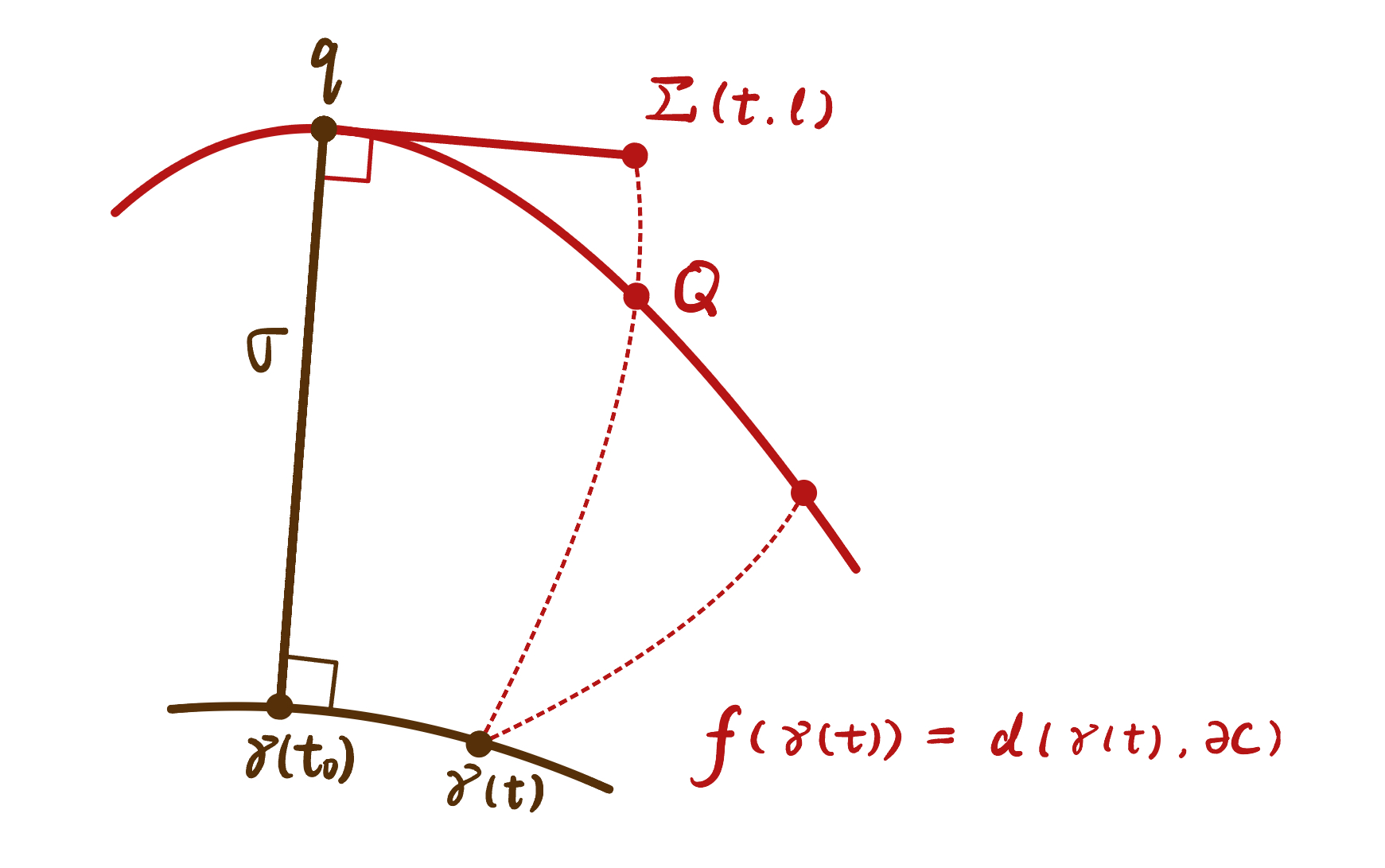
Case 2. . In this case, we need to show
We denote and the hyperplane perpendicular to at . We denote the projection vector of to . Since , the vector is below the plane as we draw in the following picture.
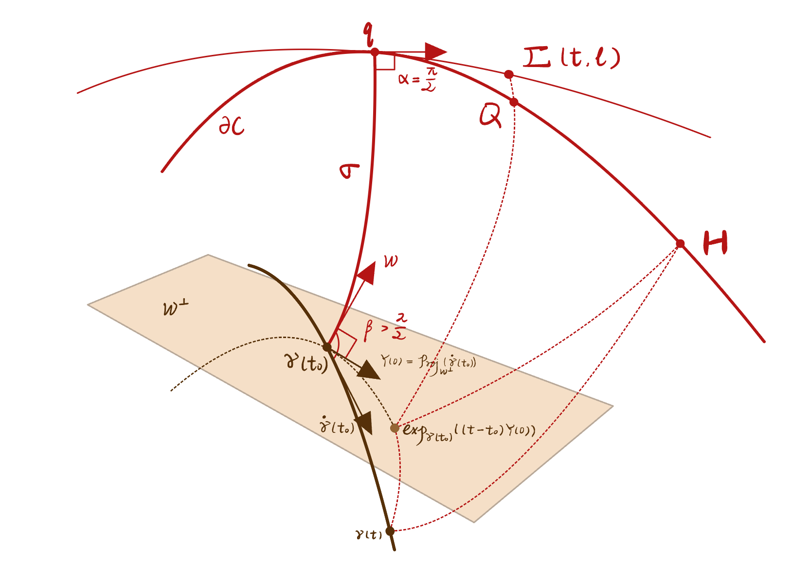
We also connected with and with the point attains the minimum distance from to . Then by the triangle inequality, we have
| (7.3) |
![[Uncaptioned image]](/html/2404.09792/assets/comparison_images/lec7image/IMG_2188.jpg)
The estimate of the first term in the inequality 7.3 is followed straight from the case when , we extend along via the parallel transport and construct the map . By the case , we know that
By the Toponogov’s hinge comparison 3.3.1, we can estimate the second term in the inequality 7.3
Therefore, we can conclude that
Case 3. . This case is similar to the case when . We connect to by a geodesic segment such that for some .
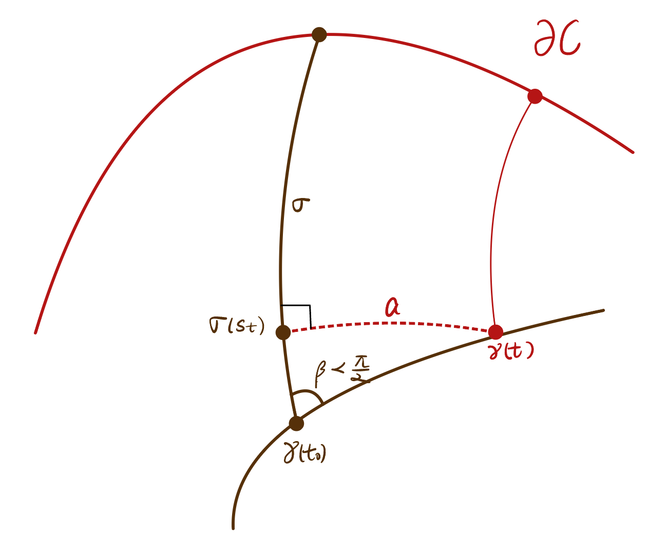
Moreover, we know that by the first variation formula, thus, from Step 1, we know that
| (7.4) |
On the other hand, by the law of cosine, we have
Also, since , we also have
Therefore, by adding the above two inequalities, we have
Therefore, the inequality 7.4 becomes,
∎
7.5 The Proof of the Soul Theorem
In the last section, we proved that the distance function to the boundary of a convex subset of a manifold of is concave on that subset. That is theorem 7.4.1. We are going to prove the soul theorem in this section.
Lemma 7.5.1.
Let be a Riemannian manifold of , a closed convex subset. We denote . Suppose there exists such that is a constant. Then there is a flat totally geodesic rectangle such that and .
Proof.
We connect and by the shortest geodesic segment . Take the unit initial vector along . If we extend to a parallel vector field along . The extension is denoted as . Then we take the exponential map along :
In particular, for .
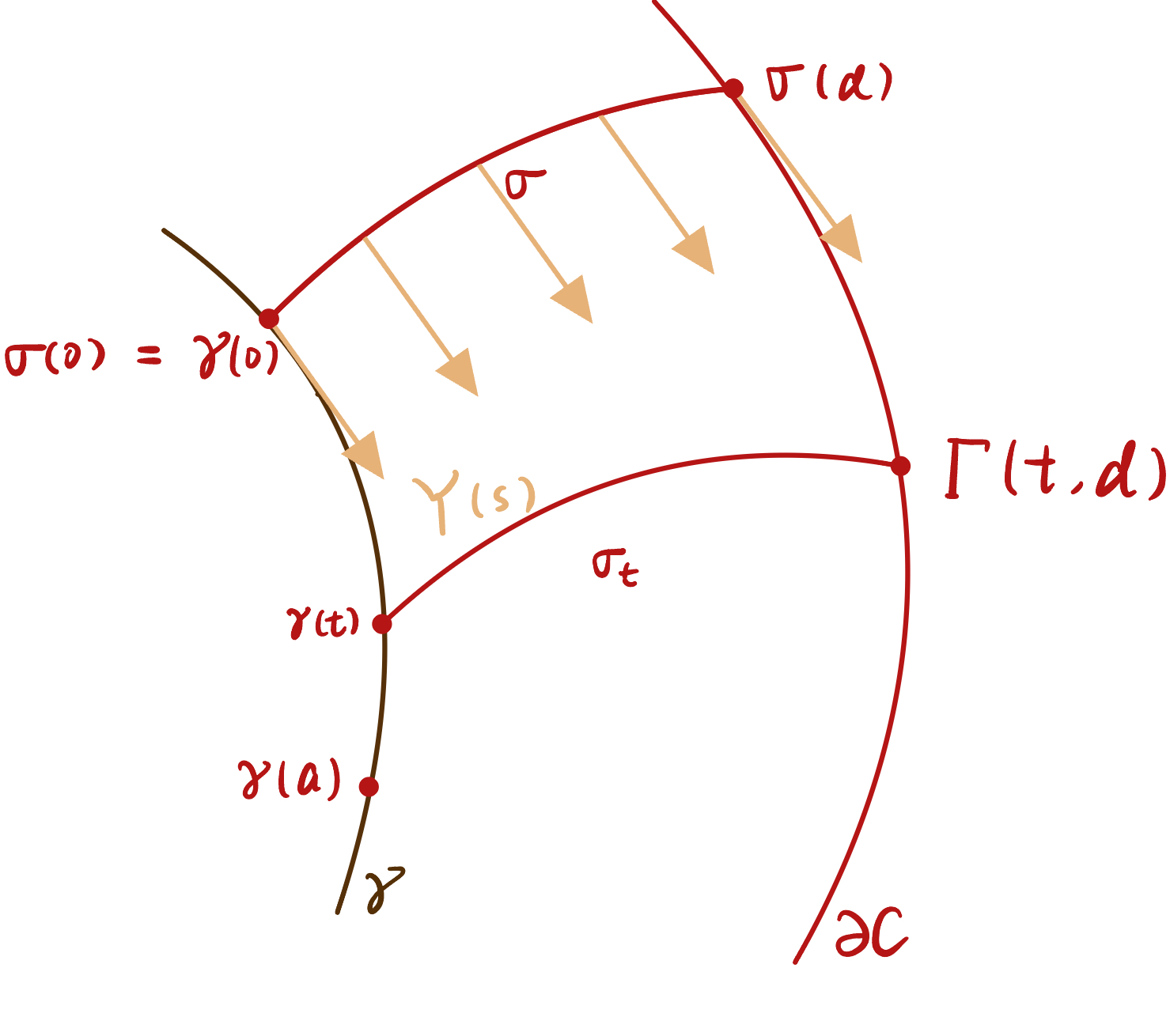
Fix , and we denote to represent the curve connecting to the boundary. , we have,
Thus all the above inequalities are equalities. Then by the Rigidity case of Berger’s comparison 3.2.3, we can conclude that
is a totally geodesic flat rectangle in and in . ∎
Now we are ready to prove the soul theorem by Cheeger and Gromoll. Let’s first recall the statement of the soul theorem.
Theorem 7.5.2 (Soul Theorem).
Let be a Riemannian manifold of and it is complete and non-compact. Then there exists a closed totally convex subset which is also a totally geodesic submanifold such that
where is the total space of the normal bundle of . In particular, has compact type since
where
is the interior of the unit disk bundle
which is a compact manifold with a boundary.
Proof.
Take and the total Busemann function at , i.e.
We know that
-
•
is concave;
-
•
The superlevel set of are compact,i.e.
is compact for every .
Thus, we can take the maximum value of . By concavity of the set is compact and totally convex. Moreover, by Proposition 7.2.23 has empty interior. Set , the maximum superlevel set. Take on . And then we take to be the maximum level set of on . And we know that is also totally convex in . Hence in . We keep going through this process until we get to an such that . We have that
The dimension goes down because has an empty interior in for each Then at some point, we must stop because we have some such that . And we denote where is the soul of . We are going to finish our proof by showing the following two claims.
Claim 7.5.3.
has no critical points on .
Claim 7.5.4.
For this ,
Proof of Claim 7.5.3.
Let . By our construction, we can find to be one of or such that lies in the manifold boundary of . we can take all shortest geodesic from to , and the initial vectors of such shortest geodesics (), then and points straightly inside. Then we can conclude that because and . We can argue by contradiction to see why this conclusion is true. If is not in the interior , then we can take and . If is concave along and This implies that by concavity. Then cannot be tangent to otherwise . Contradiction. So we can conclude that is not tangent to , then
where is the outward normal vector at to the hyperplane . Then is regular at . ∎
Proof of Claim 7.5.4.
Take a small so that
via the normal exponential map. Then the boundary of the -neighbourhood of where on and is also a manifold with boundary. And outside , has no critical points. That implies
Here we apply the Remark 5.2.30 in the critical point theory that we discussed before. ∎
∎
Corollary 7.5.5.
ad are finitely generated for any . because compact manifolds with boundaries have finitely generated homotopy and homology groups.
Corollary 7.5.6.
If , then .
Corollary 7.5.7.
If is an open complete manifold of , then and hence .
Proof of Corollary 7.5.7.
We claim that of is a point. If not, then there exists a non-constant geodesic . Fix , so that
By Propositions 7.2.23 and 7.2.22, we know that has an empty interior. So that for any ,
That means is a constant. Thus by Lemma 7.5.1 we know that there exists a flat totally geodesic rectangle parametrized by such that and . Since the is flat, for any tangent plane on , we have . Because this is totally geodesic, then by the Gauss formula the intrinsic sectional curvature equals the extrinsic sectional curvature. To see why, take tangent to .
Because,
Therefore,
In our case, is a flat rectangle, then
This is impossible since . Therefore, on the very first step in the soul construction. . Therefore, by the corollary 7.5.6, we have . ∎
7.6 Examples and Open Problems
Example 7.6.1.
If is closed and and a compact Lie group freely by isometries. Suppose further that we have a representation so that by isometries. Consider by the diagonal action. Then and its soul is .
Example 7.6.2.
Take , , admits a soul for any . Let . acts on such that and on , . So by
Then is an Möbius band and by construction, it has . The soul of is the circle .
Remark 7.6.3.
The difference between and is indeed large for noncompact manifolds.
-
•
If is open then
-
•
If is closed, if then since the manifold is closed (compact), we have a universal constant . Hence the same holds for the universal covering space , then by Bonnet-Myer’s theorem, the diameter of is finite, so must also be compact and hence is finite. In particular, admits a metric of but does not admit a metric of .
But it’s an open question is whether there exists a closed simply connected manifold which admits a metric of but does not admit a metric of .
There exist many examples of closed simply connected with and on some open dense set. In particular, such a metric exists on the Gromoll-Meyer sphere [GM74] and on [Wil02]. However, attempts to construct metrics of positive sectional curvature on these manifolds have been proved unsuccessful.
Hopf conjectured that does not admits a metric of . A more general version of Hopf’s conjecture says that if are closed manifolds then does not admit a metric of positive sectional curvature. If this conjecture is true then would provide an example of a simply connected manifold that admits a metric but does not admit a metric of . Moreover, this suggests that the above result of by Wilking is sharp.
Next, let us mention some questions related to the Soul theorem.
Given a closed manifold of and a vector bundle
in view of the soul theorem, it is natural to ask whether admits a metric of such that is a soul. This question is partially solved. For example if , then there are easy counterexamples that follow from the splitting theorem.
However, the question is still open when .
A special case of question is whether all vector bundles over spheres admit . By a result of Rigas [Rig78] it is known that this is true stably. That is, give a vector bundle there exists such that (trivial bundle) does admit a nonnegatively curved metric.
Chapter 8 Cheeger-Gromoll Soul Conjecture
In this lecture, we are going to study the Soul conjecture of Cheeger and Gromoll[CG72]. This is an essential question in Riemannian geometry about the structure of complete manifolds with non-negative sectional curvature.
Corollary 8.0.1 (Soul Conjecture of Cheeger and Gromoll).
Let be a complete open Riemannian manifold with . Suppose there exists such that near . Then the soul is a point and
This conjecture was proved by Perelman [Per94a] in 1994 in 4 pages. The proof depends on Berger’s comparison theorem 3.2.1 and the Sharafutdinov Retraction in [Sha77], which will be introduced soon in this chapter.
8.1 Distance Estimates
8.1.1 Gradients of Semi-concave Functions
Let be semi-concave and locally Lipschitz function. Then for every , the directional derivative map is defined. And
is also Lipschtiz, concave and positively homogeneous, i.e. for all (See Example 12.3.5).
Example 8.1.1.
Let be a closed subset. Let . Let . Then by the first variation formula,
Notice that this is the minimum of -Lipschitz linear functions of the form , which are all concave. Therefore is concave too. This provides an alternative explanation for the concavity of for distance functions.
Now, we want to define the gradient . We know that when is smooth then is linear and is easily defined by the Riesz representation theorem, i.e.
What about the general case?
Definition 8.1.2.
Let be locally Lipschitz and semi-concave. Let . Then a vector is called the gradient of at , denoted by , if
-
•
;
-
•
for every
Notice that if is linear, then it is not hard to show the existence and the uniqueness of in the usual sense. In general, existence and uniqueness still hold. However, this is non-trivial. And we are going to show this here.
8.1.2 Existence and Uniqueness of the Gradient for Semi-concave Functions
Theorem 8.1.3 (Existence and Uniqueness of Gradients).
The gradient in the definition 8.1.2 exists at every for locally Lipschitz and semi-concave functions and it is unique.
Proof.
We are first going to show uniqueness and then prove its existence.
-
•
Step 1: Uniqueness
Suppose and are two vectors satisfying definition 8.1.2. ThenAll the inequalities above are equalities. Therefore
-
•
Step 2: Existence
Denote .-
–
Trivial Case:
If , then on , thus we claim that is the gradient. And we just write . To check this, take , thenand
Thus we can conclude in this case that .
-
–
Nontrivial Case: If , then by the compactness of , there exists unit such that . We claim that
Claim 8.1.4.
is a gradient.
We can check that
Next, we want to check that for . To check this, we need the following lemma.
Lemma 8.1.5.
, .
We are going to verify this once we proved the existence of the gradient.
Fix , by the lemma 8.1.5, we have
Note that . Consider ,
Thus
Since we can conclude that .
-
–
Let’s verify lemma 8.1.5 above.
Proof.
Case 1: Suppose , . Since is concave we have
Case 2: Suppose , then since is concave and positively 1-homogeneous we have
That implies
∎
This allows us to define the gradient for locally Lipschitz functions and semi-concave functions and in particular for distance functions. Let’s consider the following example.
Example 8.1.6.
Take where is a closed subset in and let . We want to compute .
-
•
If is a critical point, then for any , . Geometrically, this means the angle so that . From the trivial case in the existence part of the theorem 8.1.3, this means ;
-
•
If is a regular point for , then there exists such that . Then by the first variation formula, for every , we have . By the compactness of , there exists such that attains the largest angle with . We denote this vector . Then this maximize .
Let . Now . Hence . Note that uniqueness of gradients implies that the vector is unique.
Example 8.1.7.
Let or . Then is 0 on while on the first quadrant it is given by the formula on . Then
Let us now compute the gradient of at points in the first quadrant with . By our construction
By the picture, we know that .
![[Uncaptioned image]](/html/2404.09792/assets/comparison_images/lec9image/IMG_2192.jpg)
And . Therefore
Note that .
![[Uncaptioned image]](/html/2404.09792/assets/comparison_images/lec9image/IMG_2191.jpg)
8.1.3 Gradient Flows of Semi-concave Functions
In this section, we are going to define gradient flows of semi-concave functions.
Definition 8.1.8.
Let be a Riemannian manifold and be open. Let be a function that is semi-concave on . An absolute continuous curve , where is an interval, is a gradient curve of if its right derivative satisfies for every .
The next theorem is the existence and uniqueness theorem of gradient curves. We are not going to present the proof of the existence part which was originally proved by Petrunin and Perelman in [PP95], and a simplified proof was given by Lytchak in [Lyt05].
Uniqueness will follow from Lipschitz properties of the gradient flow and we will prove this below.
Theorem 8.1.9.
Let be as above. Then for any , there is an such that there exists a unique gradient curve of , , such that .
8.1.4 More Comments on Gradients
If is a gradient curve, and is a constant then is also a gradient curve by the same argument that works for integral curves of smooth vector fields. Hence we can define the positive gradient flow where means the gradient curve starting at . Namely,
Denote . It also has the semigroup property, i.e.
This follows since for any fixed , if is a gradient curve then is also a gradient curve starting at . If , . Consider which is also a gradient curve such that , .
We see that both and are gradient curves starting at . By uniqueness of gradient curves this implies that Since for all which by above means that
Our next comment is that in general, we cannot define a flow for negative . Let on . Then
we can find the gradient flow of actually converges. The flow map is
![[Uncaptioned image]](/html/2404.09792/assets/comparison_images/lec7image/IMG_2296.jpg)
Remark 8.1.10.
Gradient flows of semi-concave functions can be defined on Alexandrov spaces where the theory is largely the same as on smooth manifolds. They can also be defined on Wasserstein spaces of Alexandrov and more generally spaces. In particular, the heat flow is constructed as the gradient flow of entropy functionals which are semi-convex (but not locally Lipschitz) in the above setting. However, the constructions of gradient flow in those settings are more complicated because unlike in the case of manifolds, we are considering point-wise gradients can not be defined, and measure-theoretic arguments are necessary.
Remark 8.1.11.
Our next comment is that if is a gradient curve, then . Hence, is non-decreasing along gradient curves. In the next lecture, we are going to prove a distance contraction estimate and show the uniqueness of gradient curves.
8.1.5 Uniqueness of Gradient Curves
Lemma 8.1.12.
Let be -concave, and . For the directional unit vector of the shortest curve from to , , we have
| (8.1) |
Proof.
Let such that and , where . By the definition of -concavity is also -concave. Therefore,
is concave. Thus
and we should keep in mind that and . Plug into the inequality, and we have
By switching the order, we have
∎
Corollary 8.1.13.
Let be -concave, . Let a shortest geodesic, then
| (8.2) |
Proof.
Proposition 8.1.14 (Distance Estimates).
Let is a -concave function, and the gradient curves of starting at and . Namely such that and . Denote
Then
Proof.
Firstly, we claim that
| (8.5) |
And if this is true, then the conclusion follows
| is non-increasing | |||
Thus, the only thing that remains to be proven is inequality (8.5). Let’s check this at , . the proof for other is the same.
Let be the mid-point of a shortest geodesic from to . That is , , and . By the first variation formula, we have
| (8.6) |
| (8.7) |
We used that
Then we add 8.6 and 8.7 together to conclude our result. By the triangule inequality, we have
which by (8.6) and (8.7) gives
Thus, we have
and by the same argument, we have
By the argument earlier this implies that
∎
Thus, we have finished our proof of the uniqueness of the gradient curves. And we are going to discuss the gradient flow.
Remark 8.1.15.
The above proof works in large generality and only needs the -st variation inequality
which is much easier to prove compared with the first variation formula. The first variation inequality holds in more general cases, i.e. infinitesimally Hilbertian spaces.
Example 8.1.16.
For example, suppose a metric measure space is . Consider the entropy function and the absolutely continuous measure. Then
is convex on ( is concave on ) where is the Wasserstein metric. And we can conclude that its gradient flow of (which is equal to the heat flow) is contracting because satisfies the first variation inequality.
8.1.6 Gradient Flow for -Concave Functions
Let be the gradient flow of such that
where is a gradient curve starting at . Then, satisfies
And by our distance estimate for -concave function, we know that
That means the flow is a Lipschitiz map with Lipschitz constant when is -concave. In particular, if ( is concave), then is -Lipschitz for all i.e. is distance non-increasing for all .
8.2 Sharafutdinov Retraction
Let’s recall the definition of strong deformation retraction.
Definition 8.2.1 (Strong Deformation Retraction).
Let be a topological space and its topological subspace. is a strong deformation retraction if there is a family of maps , such that
-
•
is a homotopy;
-
•
;
-
•
for all ;
-
•
for all .
We call the strong deformation retraction map induced by .
Notation 8.2.2.
We will abuse the notation by writing the strong deformation retraction map induced by as for simplicity.
Corollary 8.2.3.
Let be concave and is a complete Riemannian manifold. Assume all level sets of are compact. Then for any , is a strong deformation retraction, i.e. there exists a as in Definition 8.2.1.
Proof.
Firstly, we consider the case when where is the maximum value of . Let .
![[Uncaptioned image]](/html/2404.09792/assets/comparison_images/lec9image/IMG_2321.jpg)
We denote . Notice that is compact for , so we have a uniform lower bound for over this region, i.e. for every , for some constant , thus, there exists some finite time such that where is the flow map generated by the gradient vector field.
Let . Then is a bijection. We can continuously extend it to a bijection which we still denote by . then we can define the strong deformation retraction map by the formula .
-
•
is -Lipschitiz: This is because is still concave as the minimum of two concave functions. By the previous discussion, the flow map of the concave function is -Lipschitz for any (Section 8.1.6);
-
•
: This is trivial;
-
•
for . This is because on and thus is constant on ;
-
•
for all : This is because for any , is finite, thus when .
It is clear that is a homotopy. Thus we have proved the corollary for .
In general, if , then we can take for some small . And repeat the above arguments producing a family of deformations . Then we can show that is a strong deformation retraction by taking (The limits of 1-Lipshcitz maps are also 1-Lipschitz). ∎
Example 8.2.4.
Here is an example that explains why we need to consider as a separate case in the above proof. Consider such that . In this case . Thus, and . The flow map solves the following ODE:
for constant . Therefore, it takes for the flow map sending to the maximum point . By uniqueness of solutions of IVP this phenomena always happens if is smooth and .
Next, we are going introduce the corollary concluded by Sharafutdinov which is an essential construction in the proof of the soul conjecture.
Corollary 8.2.5 (Sharafutdinov).
Let be complete, . is the soul. Then there is a -Lipschitz strong deformation retraction map
Proof.
Recall the construction of the Soul. We first consider a concave function with compact super-level sets. , , where is a ray starting at .
Then is concave with compact super-level sets. Denote the maximum level set of . Then by the above corollary 8.2.3, there exists a -Lipschitz strong deformation retraction . Next, if the boundary . Then we take on and is concave. So we can take the , the second maximal level set again. As before, there is a strong deformation (by corollary 8.2.3). Then we know the soul can be found in
and remember that has no boundary. Again, we can construct the retraction. for each . We can define the Sharafutdinov retraction to be the composition of these retractions. Namely,
which is clearly also a -Lipschitz strong deformation retraction. ∎
Definition 8.2.6.
The map from the above corollary is called a Sharafutdinov retraction.
Note that at this point we don’t know if a 1-Lipschitz deformation retraction onto the soul is unique, hence for now we will say a Sharafutdinov retraction and not the Sharafutdinov retraction.
8.3 Perelman Theorem and the Soul Conjecture
Now, we can study Perelman’s proof of the Cheeger-Gromoll soul conjecture. The key is the following theorem by Perelman.
Theorem 8.3.1 (Perelman [Per94b]).
Let be complete, noncompact Riemannian manifold without boundary with . By the Soul theorem, 7.5.2, there exists which is the soul. Let be the -Lipschitz Sharafutdinov retraction in 8.2.5. Then
-
•
Part 1: For any , and any , we have
(8.8) -
•
Part 2: For any , there is a unique closest to and . In other words, is the nearest point projection onto the soul .
-
•
Part 3: Moreover, if is a nonconstant geodesic starting at , we can extend parallelly along , say , and exponentiate to a flat totally geodesicically immersed rectangle in via , i.e.
Remark 8.3.2.
Part 2 is a trivial implication from Part 1. Let , we can emanate a geodesic from to at . We parameterize by and , then By the first variation formula, we know that , thus by Part 1, we know that for all
which gives us the uniqueness in Part 2. and tells us is the nearest point projection. This shows that the map satisfying the conditions of the theorem is unique. therefore from now on we will refer to it as the Sharafutdinov retraction.
8.3.1 The Proof of the Soul Conjecture
Using this theorem 8.3.1, the soul conjecture is an easy corollary.
Corollary 8.3.3 (Soul Conjecture of Cheeger and Gromoll).
Let be a complete open Riemannian manifold with . Suppose there exists such that near . Then the soul is a point and
Proof.
The proof uses the Sharafutdinov retraction .
![[Uncaptioned image]](/html/2404.09792/assets/comparison_images/lec9image/IMG_2193.jpg)
The existence of the Sharafutdinov retraction follows from the corollary 8.2.5. And by 2. in the Perelman theorem 8.3.1, there exists a unique closest to such that . Suppose . Then we can take a nontrivial geodesic in starting at . Then by 3. in Perelman’s theorem 8.3.1, we can obtain a flat totally geodesic rectangle . The above picture shows that at the top right corner. Thus, if is a -dimensional plane at tangent to , then because is flat. However, this contradicts the fact that near . So and therefore,
∎
8.4 The Proof of Perelman Theorem
Define a function such that where is the Sharafutdinov retraction.
In particular, when and , we have on all the zero sections. This implies that for any such that , we have
| (8.9) |
because is -Lipchitz and .
8.4.1 Perelman Theorem for Small (Part 3.)
We first consider the case when is small, i.e. . In this case, we define a map such that for each ,
One readily checks that has the following properties
-
•
;
-
•
by 8.9;
-
•
.
Because , we connect to via the shortest geodesic and we can extend a little past to some point so that it remains shortest. Because the three points lies on the same shortest geodesic, we have precisely
Now, we extend to a parallel vector field along and denote the vector at by . Then, we can project both and to by . This gives us the triangle .
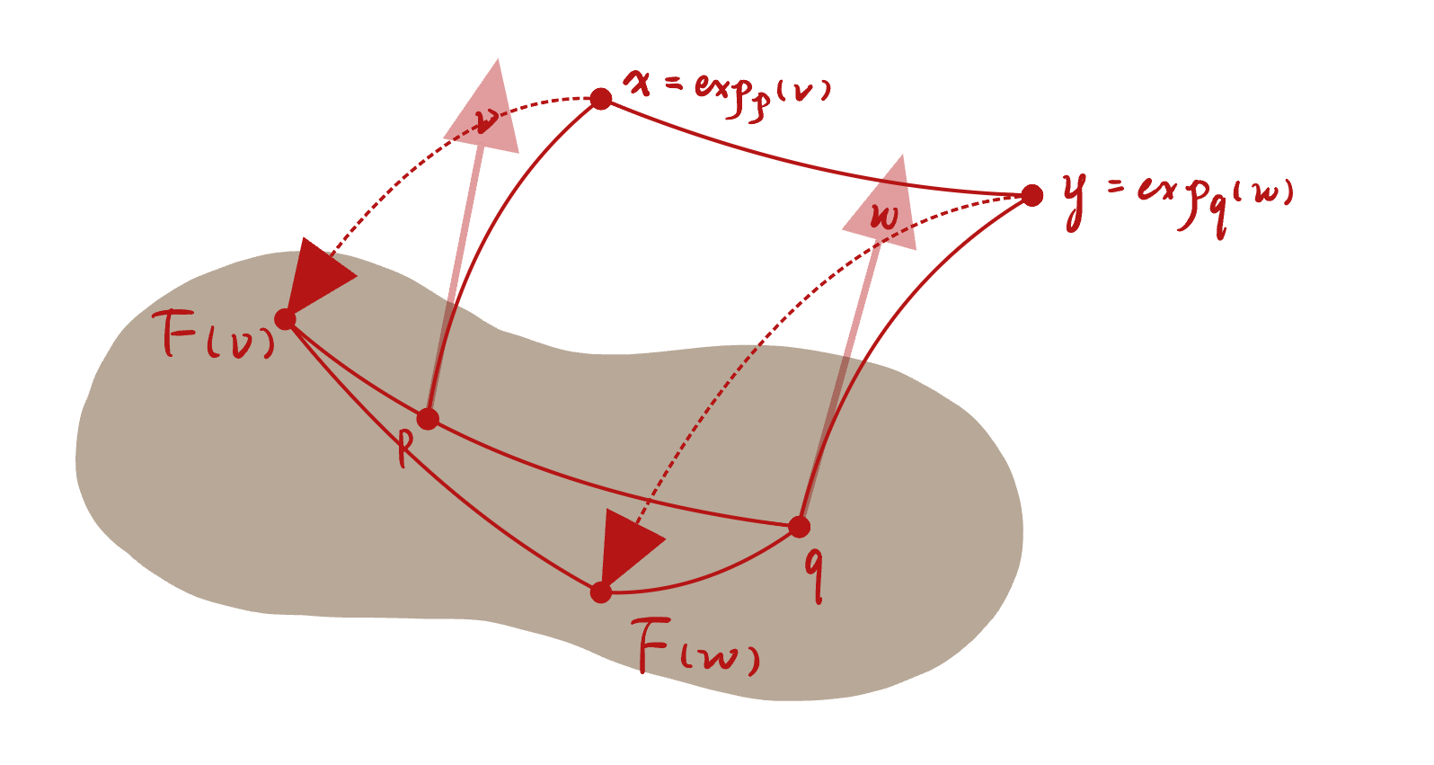
By the triangle inequality, we have
| (8.10) |
By the maximality of the choice of , we know
| (8.11) |
On the other hand, we can check that
| (8.12) |
This is because
Next, we can continue the triangle inequality 8.10 by the estimates 8.11 and 8.12
We find the inequalities above must be equal! In particular, we conclude that
| (8.13) |
By the rigidity case of Berger’s comparison equality 8.13 tells us that is a flat totally geodesic rectangle.
8.4.2 Perelman Theorem for Small (Part 1.)
The following lemma implies the 8.8 directly.
Lemma 8.4.1.
. Then by the properties of , we can conclude that for all small .
Proof.
We prove this lemma via the perturbation method. Pick small some , and define a vector slightly shorter than , i.e. . Thus
![[Uncaptioned image]](/html/2404.09792/assets/comparison_images/lec9image/IMG_2194.jpg)
By the triangular inequality
Still, by the definition of , we have
Thus
| is nonincreasing |
Since and we can conclude that for all small . ∎
Remark 8.4.2.
Notice that it is possible that the above inequality
is a strict inequality. This is because the rectangle is not necessarily convex so the shortest geodesic of the rectangle is not necessarily the shortest geodesic in the manifold.
8.4.3 Perelman’s Theorem for Large
The proof of the equality 8.8 can be generalized to large in [Per94a]. Let
We want to show that . Suppose . Then for small we have that for any a unit vector it holds that .
Then Lemma 8.4.1 shows that there exist a small such that on . This means that is not the maximum. Therefore, .
8.5 Regularity of Sharafutdinov Rectraction
The proof of the Perelman theorem implies that the Sharafutdinov retraction is a submetry, which implies some regularity of . What we mean by a submetry is rigorously defined below.
Definition 8.5.1 (Submetry).
Let and be two metric spaces. Then is a submetry if
(Notice that submetries are -Lipschitz by definition.)
Example 8.5.2.
Here are some examples of submetries.
-
•
The first coordinate projection from to is a submetry.
-
•
Any Riemannian submersion between two complete and connected Riemannian manifolds is a submetry. Let be a Riemannian submersion where and are complete. By the definition of a Riemannian submersion, it is trivial that
Now we want to show
This is because we can lift the geodesics horizontally. Fix , Denote by the shortest geodesic from to parameterized by its arc-length . We can lift horizontally to starting at , there is and such that
-
–
for each ;
-
–
and ;
-
–
The last point implies that
therefore, we can conclude that
so that is a submetry.
In fact this shows that since the 1-Lipschitz condition implies that . This means that the fibers if are equidistant and the distance between them is equal to the distance between their images. That is given for any it holds that . This property more generally holds for all submetries, not just Riemannian submersions.
-
–
-
•
Suppose is a compact group acting on by isometries where is a complete geodesic metric space. Take . Then the orbits of this action are equidistant and admits a natural quotient metric and the projection is a submetry.
We used the following result by Guijarro and Walschap as a fact.
Theorem 8.5.3 (Regularity of Submetries between manifolds [GW09]).
Suppose is a submetry between two smooth compact Riemannian manifolds. Then is a -Riemannian submersion, where means are locally Lipschitz in coordinates.
Remark 8.5.4.
The regularity in the above theorem is sharp and can not be improved in general.
Proposition 8.5.5.
The Sharafutdinov retraction in theorem 8.3.1 is a submetry
Proof of Proposition 8.5.5.
It is easy to see that since is -Lipschitz. Now we want to show . Firstly we denote and fix such that . To show we take as the shortest geodesic from to and we know that . Also, we take to be the shortest geodesic from to .
![[Uncaptioned image]](/html/2404.09792/assets/comparison_images/lec9image/IMG_2195.jpg)
Then by Perelman’s theorem 8.3.1, we have a flat totally geodesic rectangle with sides and . Then by the picture, we know that there is such that and .
This is equivalent to say . ∎
Combining the claim 8.5.5 and the regularity result of submetry 8.5.3, we can conclude the following corollary.
Corollary 8.5.6.
The Sharafutdinov retraction in the Soul theorem is a Riemannian submersion.
Indeed the full regularity result that is is proved by Wilking in 2007 [Wil07]. This is a very difficult result and we are not going to prove this in the lecture.
In the Soul conjecture 8.3.3, we know that is diffeomorphic to . Does that mean the normal exponential map is a diffeomorphism? The answer to this is NO. The map is generally not a diffeomorphism even when . Consider the following example.
Example 8.5.7.
Take to be a surface obtained by rotating the parabola around the -axis. This surface has . And the Soul of the surface is . Now the normal exponential map is a diffeomorphism.
Now we deform this metric to be slightly bumpy and still keep the sectional curvature strictly positive. This is possible since the curvature of the paraboloid of revolution is positive away from the origin. Then there exists a with non-unique shortest geodesic from to and that makes the exponential map no longer diffeomorphism.
In this example, because , thus is the normal bundle. We should learn from this example that does not imply that the normal exponential map is a diffeomorphism.
Chapter 9 Cheeger-Gromoll Splitting Theorem
We now going to move to our next topic - The splitting theorem of the manifolds of non-negative sectional curvature. The initial version of the splitting theorem is proved in the same paper of Cheeger-Gromoll where they proved the Soul theorem.
Theorem 9.0.1 (Splitting Theorem by Cheeger-Gromoll).
Let be a complete open manifold with and contains a line (global geodesic) such that
Then there is an isometric splitting on
where also a complete open manifold with .
Example 9.0.2.
Consider where in this case are just the vertical lines for each .
Remark 9.0.3.
The splitting theorem 9.0.1 also holds for Alexandrov spaces of nonnegative curvature (We will study Alexandrov spaces in Chapter 13). The proof of the splitting theorem in the setting of nonnegative Ricci curvature manifolds can be found in [EH84, CG71]. The splitting theorem for space was also discussed in Gigli’s lecture in Fields Institute in the Fall of 2022 [Gig22].
9.1 The Proof of the Splitting Theorem in the Smooth Setting
Let be a line. We can define two rays , i.e. for all and for all . Then, we can associate the corresponding Busemann functions and to them. Remember that and are concave -Lipschitz. Firstly, we claim that on .
Lemma 9.1.1.
on .
Proof.
For any , we have
Therefore, for any , by the triangular inequality, we have
Notice that this gives us
By taking limits , we got
∎
Lemma 9.1.2.
In particular, we have
Proof.
We first consider the case when , In this case,
and
Thus,
The proof for is exactly the same. ∎
Denote
We notice that is concave, nonnegative, and (since ).
Proposition 9.1.3.
on
There are two approaches to proving this lemma, the first one relies on the extendability of a geodesic in the complete Riemannian manifold. This approach relies on the smoothness of the space. Nevertheless, the second approach doesn’t, which therefore can also be applied to the setting of Alexandrov space.
Proof of Proposition 9.1.3 (Method 1).
We only need to show the following statement:
Let be a complete Riemannian manifold and be a concave, non-negative function. And, we require for some . Then .
Let . Let be an infinite geodesic such that and . Then is concave, nonnegative, and vanishes at 0. Since
And because is non-negative, we must have
We therefore can conclude that . ∎
Proof of Proposition 9.1.3 (Method 2).
We know that is -concave since , i.e. is concave in . And we know that every concave function linear function. Thus, there exist such that for any
Also, we have that
Then we can add them together such that
Since ,
We notice that
This means, on . However, we already know that by the lemma 9.1.1. Thus, we can conclude . ∎
The advantage of method 2 of the proof is that unlike method 1 it does not rely on existence of bi-infinite geodesics in all directions and generalizes to Alexandrov spaces.
Since both and are concave, then and are convex. However, since , these two Busemann functions are both concave and convex. Therefore, they are affine. That means for any geodesics in ,
for some constants and .
Lemma 9.1.4.
The set is totally convex in for every
Proof.
Since
Therefore, their intersection
is totally convex. ∎
Remark 9.1.5.
However, the intersection of two convex subsets is not necessarily convex. In fact, the intersection is not necessarily connected. By Figure 9.1, and are both convex subsets of . However, their intersection is just a set containing two points.
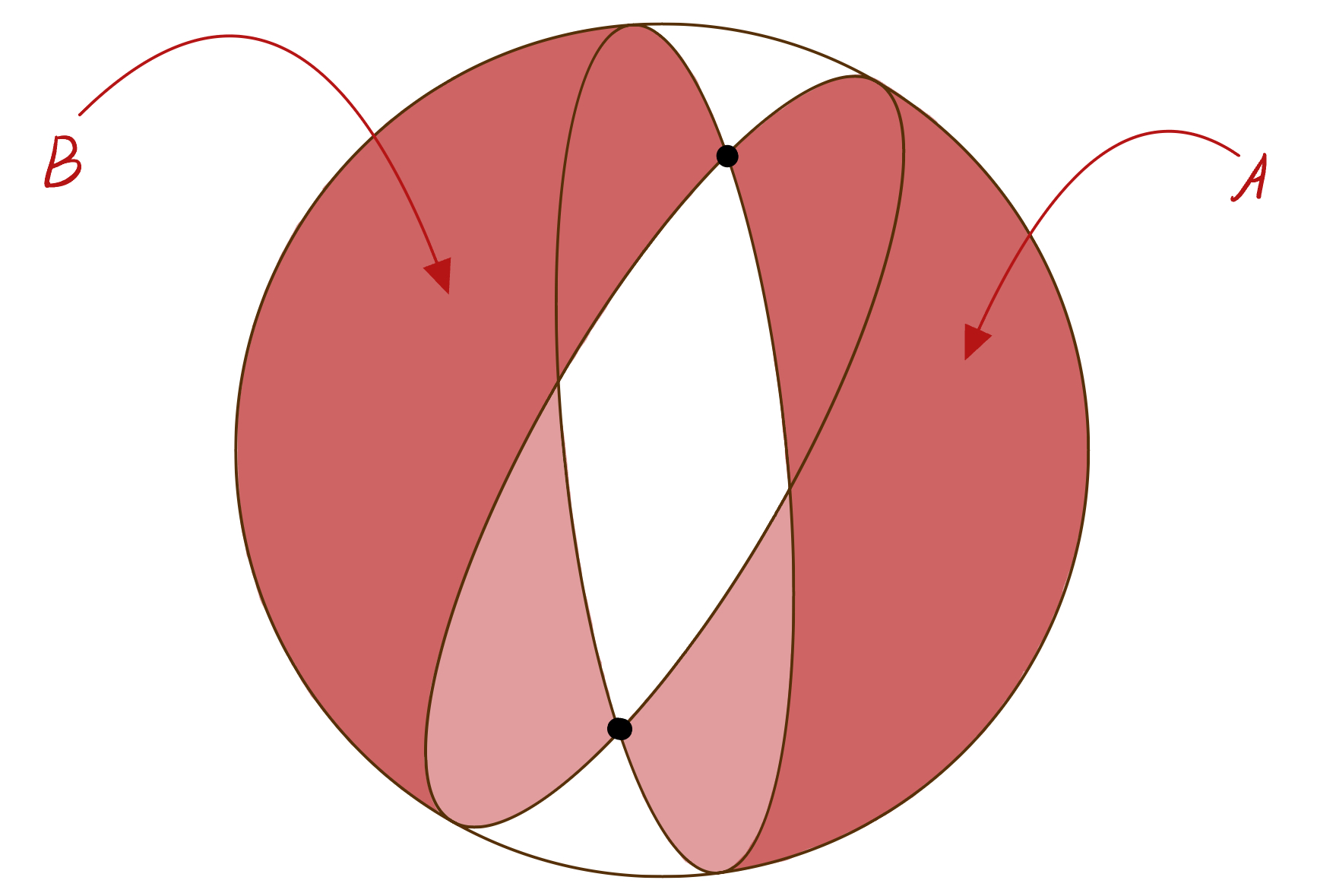
9.1.1 The Construction of the Gradient Flow
Recall that both and are affine. Therefore if and is a geodesic passing through then on , Therefore the convex set is a totally geodesic submanifold without boundary.
Denote and be a pair of negative gradient rays of and respectively starting from . Since for every ,
and (By proposition 9.1.3), we have
and
We summarize the results here
-
•
-
•
-
•
-
•
Now, let’s construct the joint curve
| (9.1) |
So along , because are -Lipschitz
| (9.2) | ||||
| (9.3) | ||||
| is the gradient curve of | (9.4) |
and
| is the gradient curve of |
Denote and the gradient flows for and respectively. The lines are trajectories of the flows passing through . Because for every -line such that .
we can say that ,
Moreover, because both and are concave, both and are 1-Lipschitz. However, . Then ,
Therefore, all the inequalities are equal. Thus
Therefore, we can define an isometric global flow
This is clearly a flow since
9.1.2 The Flow Maps are Bijective
We can think of it as the gradient flow of but defined on all of as opposed to only. By above we have that increases with speed 1 along the flow . That is
Similarly increases with speed along its gradient flow . By Lemma 1.3.6, for each , the curve is a line as are the unit speed gradient curves for respectively.
Let’s look at the map where we define . For each
Because our manifold is foliated by the gradient curves of it easily follows that is a bijection since all of our flow maps are invertible.
Suppose . This means . Applying to both sides gives . We have and . Hence , and hence . This shows that is 1-1. Now we want to show is onto. Let , we want to show there exists and such that . Let , and consider the line passing through , by applying , we have
thus we know that thus we can conclude that
9.1.3 The Flow Maps are Isometries
Now we only need to verify that to is an isometry. Assuming we know that is , we can conclude the argument as follows. Consider the map
For any fixed look at the map . Since is an isometry this map is an isometry as well and the same is true for its differential at any point in . Also, we know that is a line orthogonal to the level sets of . In particular, its derivative is a unit vector for any . Note that the tangent space is a direct orthogonal sum of and and by above the differential preserves their orthogonality and is an isometry on each component. Thus is a block-diagonal matrix with each block an orthogonal matrix. Hence is an isometry. Since is arbitrary and is a bijection this means that is an isometry. And thus we finished the proof.
Therefore, is an isometry and .
Remark 9.1.6.
The arguments in the last part of the proof only work if we know the flow is smooth (at least ). It can be shown that this is the case in our situation but we are going to present a different argument that does not rely on the smoothness of the flow and works on Alexandrov spaces and not just on the Riemannian manifold.
Remark 9.1.7.
The splitting theorem in space is much harder to proof because the lower Ricci curvature bound is rather a weak assumption.
9.2 The Proof of the Splitting Theorem in the Non-Smooth Setting
In the last lecture, we proved the splitting theorem for nonnegative sectional curvature Riemannian manifolds. However, the proof last time can only be made of only when the flow is . Therefore, we need an alternative proof to generalize the theorem to Alexandrov space of nonnegative curvature in this lecture. Still, our goal of this section is to show is an isometry.
9.2.1 Petrunin’s Estimate
Recall from the last section, we already show that is a bijection. And we know for each , is an isometry from to itself. This means if we define , the restriction map
is an isometry.
However, this only shows that preserves distances between points in the same slice, i.e. for , we have .
What if and are in different slices where and ? This is nontrivial. To estimate the distance between and . We need the following proposition by Petrunin.
Proposition 9.2.1 (Petrunin).
Let be a Riemannian manifold with . Let be a -Lipschitz and concave function over . And the gradient flow of for . Let and . Then
| (9.5) |
The proof of Petrunin’s estimate will be given in the next section. In this section, we want to apply Petrunin’s estimate to show is an isometry. Indeed, it is enough to show that
for , .
The key point here is to apply Petrunin’s estimate applies both to the flow where which is the gradient flow of and to the flow where which is the gradient flow of .
Without loss of generality, suppose , then
As we mentioned in the beginning, is an isometry. We therefore have
Therefore it is enough to prove the case when , , i.e.
| (9.6) |
To verify equation 9.6, we apply Petrunin’s estimate to both and . Since we assume , we have (corresponding to and )
Thus, by applying Petrunin’s estimate twice to both and , we have
This is because are the gradient flows of and . And remember that are zero on .
Thus, all the inequalities above are actually equalities. In particular, we have
By rearranging the terms and the square root, we prove that the equality 9.6 is true.
Remark 9.2.2.
The equation 9.5 is an equality for the Busemann function on or more generally if we consider and the geodesic passing through . Then for , the equation 9.5 admits the equality. Here we check that. Denote and , then
So and . Then we can write
That means equation 9.5 can be written as
where and . So that is the gradient flow of on .
9.2.2 The Proof of Petrunin’s Estimates
Let , otherwise, just flip the roles of and . It is enough to prove the inequality 9.5 for . Since ,
Now, it is enough to prove the inequality 9.5 for from above. Equivalently it is enough to prove the inequality 9.5 for for . Namely, we want to show
| (9.7) |
Notice that is the gradient flow passing through , denote . Then the left hand side of the inequality can be denoted as . Consider
| (9.8) |
Let be the geodesic from to , then . Then we have the first variantion formula, which implies
| (9.9) |
Recall that for the geodesic between and and is concave, we proved before that along , we have
Apply this to the inequality 9.9, we have
So apply this to the inequality 9.8, we have
Remember that is -Lipshchitz, we have because
Therefore,
Then we finish the proof since
Chapter 10 Cheeger-Gromoll Covering Theorem
We are going to study the space of the isometries of the non-negatively curved manifolds.
10.1 Preliminaries
Definition 10.1.1.
Let be a subset of and a group acting on , then we denote the family of the orbits of .
Definition 10.1.2 (-invariant).
Let be a subset of a Riemannian manifold, and be a group. Then is called -invariant if for any and any it holds that .
Lemma 10.1.3.
It is easy to check that is -invariant.
Proof.
For each , . ∎
Definition 10.1.4 (Totally Convex Hull).
Let be a subset of a Riemannian manifold , we denote the closed totally convex hull of if it is the smallest closed totally convex subset of containing .
10.2 Introduction to the Covering Theorem
Theorem 10.2.1.
Let be a complete Riemannian manifold of . If
and has no lines, then the isometry group is compact. Moreover,
i.e. any isometry looks like where is an isometry of and an isometry of .
There are several statements that we need to show here. The first one is to show is compact. Then we will use this theorem to prove the following theorem:
Theorem 10.2.2.
If is a compact Riemannian manifold of , then its universal cover is isomorphic to where is also of . And a finite cover of is diffeomorphic to . In fact, up to finite index is just
The first theorem we want to prove is
Theorem 10.2.3.
If has no line and satisfies , then is compact.
For proof, we need the following proposition
Proposition 10.2.4.
Let be a complete open manifold with , be a compact subset. Let and let be the closed totally convex hull of i.e. the smallest closed totally convex set containing where is . Then there exists finite such that .
Proof of Proposition 10.2.4.
The first thing we need to claim is that is also -invariant. Let . Since is the closed totally convex hull of and it follows that is also a closed totally convex subset containing . Since is the smallest of such sets, then . Applying , we have
Therefore, we actually have
And this means is -invariant.
We next claim that for any and ,
Let be such that
Such exists since. is closed. Since is an isometry, we know that
Then,
To show the opposite inequality, we can apply , so that
Therefore, all the inequalities are actually equal. Hence our second claim is also true.
Suppose it is not true that there exists a finite such that . That means we can construct a sequence of such that
By our claim above, we know that
for each as well. For each , denote the closest point to .
Then by the compactness of , by passing up to the sub-sequence, and segments produce a ray starting at such that
Note that the whole segment is contained in and since is closed this implies that the entire ray is contained in as well.
Take the corresponding Busemann function. We can check that
this is because for each ,
Hence, take some , the set is a closed totally convex subset containing . This means that the set . Hence, considering . On one hand, we have
However, we know the entire ray is contained in , thus in particular . Contradiction! ∎
Remark 10.2.5.
Without the assumption of , the totally convex hull need not lie in
Corollary 10.2.6.
If is non-compact, then contains a line.
Proof of Corollary 10.2.6.
Suppose that is non-compact, then the closed totally convex hull of must be non-compact as well. By Hopf-Rinow theorem must be unbounded since, in complete manifolds, closed bounded sets are compact.
Since is also convex, this means it must contain a ray, i.e. for each point , there must be a ray, say starting from , such that . Indeed, since is unbounded we have a sequence of points such that and the shortest geodesic segments going to sub-converge to a ray (since the directional vector start from sub-converge in the unit sphere).
![[Uncaptioned image]](/html/2404.09792/assets/comparison_images/lec9image/IMG_2199.jpg)
Recall that . Hence, for each natural number , . This means there exists such that .
Notice that
Taking , and we can shift to such that . Notice that now
![[Uncaptioned image]](/html/2404.09792/assets/comparison_images/lec9image/IMG_2200.jpg)
This means for any .
Since is compact, by passing to a subsequence we can make sub-converge to a line . ∎
Corollary 10.2.7.
If is complete with and has no lines, then is compact.
Proof of Corollary 10.2.7.
Let be a point in , which is certainly compact. Suppose is non-compact, then is non-compact. Otherwise, the whole group is compact because and the isotropy group of is compact. Indeed, any is determined by and . In particular for the map is determined by (the orthogonal group in the tangent space.). And since is a closed subgroup of which is compact it follows that is also compact. So is non-compact. Hence, if is non-compact, by the previous corollary 10.2.6 with , has a line. So contradiction. ∎
So far, we can conclude that when has then
And we know that
| If has a line | |||
| (splits) | |||
| This implies that translations along factor are isometries. | |||
| is non-compact |
Now, let’s summarize everything in a theorem
Theorem 10.2.8.
Let be a complete Riemannian manifold with . Then
-
1.
where has has no lines and is compact. This splitting is unique in a strong sense. Namely, if is an isometry, for , , then where , the factors and are uniquely determined and do not depends on the choice of .
-
2.
. Namely, if and then is an isometry. This result means all the isometries of are like this.
Let’s quickly explain 1. and then prove 2.. The only thing that is left to be proved is the uniqueness of the splitting factors.
Let be a line. Then where and are geodesics in and respectively. Suppose is not constant. Then cannot be globally shortest. Eventually, this means is not minimizing, i.e. there are such that the segment can be replaced by a shorter curve, which implies is also not shortest. Contradiction! This means that for some and is a line in . Now, since is an isometry it sends lines to lines. Hence the above discussion tells us that . So . Since isometries preserve angles between vectors this implies that geodesics orthogonal to the factors must map to geodesics orthogonal to factors. Hence . This finishes the proof of 1.
Proof of 2. in theorem 10.2.8.
Since is isometric to to understand its isometry group we can just assume that . It is sufficient to consider . Remember how this map is constructed, for and , we have
This is an obvious homomorphism. We want to show that is moreover a bijection.
-
•
is one-to-one: This is obvious.
-
•
is onto:Let , maps lines to lines, factors to factors and factors to factors isometrically. Fix , , then
is an isometrically embedding onto . Also,
is an isometrically embedding on to some . The linear map looks like where and are both isometries and . Hence, we can have isometry such that and isometry such that . If we take the isometry and . Then since two isometries that have the same values and the same differentials at a point must be equal.
Therefore which proves that is onto.
∎
Theorem 10.2.9 (Cheeger-Gromoll Covering Theorem).
Let be compact and , then the universal cover where is compact and simply connected. And a finite cover of is diffeomorphic to
Remark 10.2.10.
Warning: It is not true that the finite cover must be isometric to . It is in general only diffeomorphic.
Example 10.2.11.
Take . And is -actions, i.e. acts on by translations in standard way: . Moreover, we take the action on to be irrational rotation around the -axis, i.e. take irrational, so that the order of the rotation .
![[Uncaptioned image]](/html/2404.09792/assets/comparison_images/lec9image/IMG_2201.jpg)
Take the diagonal action of on , i.e. , . More explicitly, if , then . Let . Then is compact, and the universal cover is just isometrically, but not isometric. Moreover, no finite conver is isometric to since is irrational and the rotation can never be equal to identity for .
10.3 The Proof of the Covering Theorem
let be the universal cover of . Then where has no lines and compact isometry group.
Claim 10.3.1.
is compact.
Let by deck transformation. but . Then acts diagonally
For , then
Remark 10.3.2.
isometry, then , such that .
We have diagonally. We are given that is compact. For let . It is a closed subgroup of which is compact and hence is compact too. We have . Since is compact this implies that is compact too. Since is compact this implies that is compact as well. So we can conclude that
Let , acts trivially on and acts freely and properly discontinuously on . This action must be free since acts freely on and the action of on is trivial. But is compact. is closed manifold, freely & properly discontinuously. Therefore, is finite, otherwise, the action would not act freely and properly discontinuously. Indeed, If is not compact, has an accumulation point and the action is not properly discontinuous. Thus is a finite subgroup. Let . Notice that is compact but not simply connected unless i trivial. Then which is finite and acts diagonally in and .
Claim 10.3.3.
A finite cover of is diffeomorphic to .
Note that . has a finite cover diffeo to . Hence this claim implies our theorem.
It is remain to prove this claim. We have action, and and but now this is injective, therefore,
is a discrete subgroup. The quotient must be compact. Otherwise, as before, we get that is also non-compact which we know is false. Also, the discrete subgroup of and is compact. By Bieberboch Theorem, a finite index subgroup generated by translations by linearly independend vectors in . , , then
. By passing to a finite cover of , we have acts on diagonally action on translations generated by basis of . Then .
Consider
Let , so is Abelian, then is Abelian Lie group, is compact. Let be the identity component of , which is compact, Abelian and connected. Therefore, for some . And since is compact and hence has finitely many components. Take , then finite index subgroup. then the image of finite index subgroup of is isomorphic to .
still acts cocompactly. Consider . It is a the finite cover of and it is enough to understand .
Claim 10.3.4.
to show this claim, consider
Also is a cocompact lattice.
Observe that we can extend the homomorphism to a homomorphism
To see why, it is enough to check the extension of one of the component of . Namely, we only need to extend to . This is easy since everything here is Abelian. So if , we have
Set by the formula, , . It is easy to see this is a homomorphism. Now we get extending to still homomorphism. Now we can produce a diffeomorphism as follows.
First look at
given by
This is a diffeomorphims since we have the inverse map
Claim 10.3.5.
is equivariant if we take the diagonal actions of on the target and on the domain, we just take the action on .
on the second factor only . In other words we claim that
i.e. is equivariant. , . This means passes to a quotient by . This we get diffeomorphism (diagonal action, finite cover of ). Therefore, is a diffeomorphism where is the finite conver of .
Chapter 11 Bishop-Gromov Volume Comparison
In this chapter, we are going to state and prove the classical Bishop-Gromov volume comparison theorem.
Lemma 11.0.1.
Let be a monotonous non-increasing function. Then the average integral
must also be non-increasing.
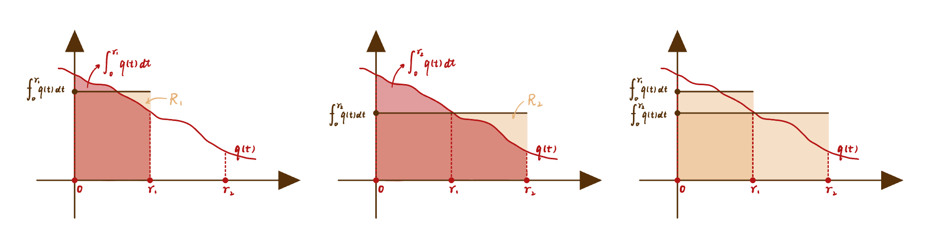
Proof.
Indeed, for
Notice that and . Also notice that since is non-increasing, then
Therefore,
for . ∎
Theorem 11.0.2 (Bishop-Gromov Relative Volume Comparison ).
Let be a complete manifold with . Recall that denotes the complete simply connected -dimensional space of (thus ). Let and . Then the function , where
| (11.1) |
is non-increasing with respect to .
Relative volume comparison has the following immediate corollary
Corollary 11.0.3 (Absolute Volume Comparison).
Under the assumptions of Theorem 11.0.2 for any it holds that
Proof of Corollary 11.0.3.
Because is asymptotically Euclidean for small ( since ) we have that
Now monotonicity of immediately implies the result. ∎
Proof of Theorem 11.0.2.
Denote by the volume form on and we want to compute the volume form in exponential coordinates. For each , , thus we can define polar coordinates on . Namely, if and , then
is the polar coordinates. Take . Thus
We can pull back the volume form by .
Remark 11.0.4.
Let’s recall the definition of the pullback: For , , is the basis. Thus we can define the pullback as
Consider which is parameterized by and consider , where is the unit vector at the origin. Then . Let be the orthonormal basis of . Since has the volume form , i.e. for the volume form , there exists such that
We want to understand . By the definition of the pullback form
By the definition of , we know that
On , . For vectors , we apply to them. Look at the Jacobi fields in the flat metric on given by . , which are normal to . Then
is the Jacobi field along satisfying the initial conditions .
Remark 11.0.5.
Recall that Jacobi fields that vanish at can be obtained by taking the variation of the exponential map. Thus we denote . And also . Notice that for all . Recall that if is Jacobi along . Then
In our case, , .
So we have . Now by the definition of , we know that
Therefore,
which is just the volume of the cuboid spanned by .
Remark 11.0.6.
If in , are orthonormal basis of , we can write the column vectors in this basis, then
Therefore, let be parallel vector fields along , . Start with , and . Therefore, we can write as colume vectors with respect to the orthonormal basis . And in the basis , we have
Then , which is the determinant of the -block. Remember that for
we have
. Therefore,
Recall the Jacobi equation along
can be split into
where satisfies the initial condition as .
Then
We will only need , i.e. is shortest on . That implies there are no conjugate points on . Therefore, are linear independent for all (This is a basis of and we can write as a matrix in this basis.).
Since
Then we can take the trace on the matrix equation . We get
| (11.2) |
Notice that
-
•
;
-
•
;
-
•
. where is defined as and . Then . And the inner product on square matrices is defined as . We can check that under this inner product:
Therefore, we can write the equation 11.2 of the trace of the shape operator as
And now we have a Riccati equation on the scalar function . Notice that we have as because as . Remember that is the solution of and on the interval of existence. (The interval of is bigger.) Therefore, .
Remark 11.0.7.
In the case of the model space . , . So we get equality on .
By Riccati comparison, before the first conjugate point along . Just as in Rauch’s comparison, we get an inequality on and . Therefore, we have
| is non-increasing | |||
Therefore, up to the first zero of which must occur before the first zero of . So
and
Then we can conclude the following
-
•
If , then for ;
-
•
If , then the first zero of is . Therefore must have a zero before . Which means that the first conjugate point along occurs before . This immediately gives.
Corollary 11.0.8.
If , then .
Let’s collect what we have so far. For , , . Because is a unit vector, such that is shortest on . ( could be but for compact manifolds ).
We know that is a diffeomorphism.
Fact 11.0.9.
has measure , for computing volumes is irrelevant
So is a diffeomorphism (This is for computing volume). For computing volume, we just want to use this part of the map. In short,
Let’s redefine to be for . And do the same for :
-
•
If , then for (Don’t need to redefine );
-
•
If , then . We set it to be zero for
Recall the first zero of is than the first zero of , then is still non-increasing with this definition, for , we set it to be zero. Then we have redefined and .
Since we can express
and
Thus, we have
where we denote . Since we know that is non-increasing for all and is also non-increasing concerning . Thus the ratio is also non-increasing. This is because
| (11.3) |
and the integrand is non-increasing (by Lemma 11.0.1), where the measure on and for . ∎
Chapter 12 Gromov-Hausdorff Convergence of Metric Spaces
In this section, we are going to introduce the Gromov-Hausdorff topology. This concept is generalized from the Hausdorff topology for metric spaces. The reason that we need this generalized concept is that we want to study a family of compact Riemannian manifolds, or more generally, a family of metric spaces, sharing the same properties on curvature bound, volume bound, and diameter bound, for example, the family of Riemannian manifolds
We will see that this class is pre-compact in Gromov-Hausdorff topology. This fact has a number of interesting applications.
12.1 Hausdorff Distance
Let us briefly review the Hausdorff distance here. The Hausdorff distance allows us to measure the distance of two subsets intrinsically from the point of view of metric. Intuitively, the Hausdorff distance gives us the least radius that we can shrink one subset to touch another subset.
Notation 12.1.1.
For a metric space , and a subset . For any , we can denote the distance from to as
Definition 12.1.2 (-neighborhood).
Let be a metric space and . For , we can define the -neighborhood of as
where is called the radius of the neighborhood.
Definition 12.1.3 (Hausdorff Distance).
Let be a metric space, and let be subsets. The the Hausdorff distance of and , denoted by , is defined as
| (12.1) |
where and are the -neighborhood of and .
We can provide an equivalent definition of the Hausdorff distance by thinking of the smallest radius of the neighborhood of covering as the largest distance from some point of to (See Figure 12.1). That is
Definition 12.1.4.
Let be a metric space, and be subsets, the Hausdorff distance of and can also be defined as
| (12.2) |
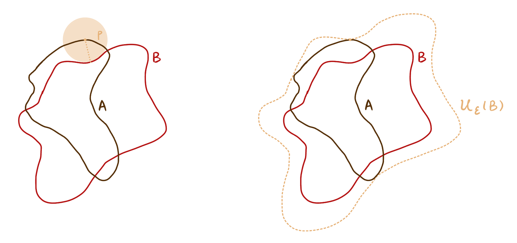
Remark 12.1.5.
It is possible that the
Proposition 12.1.6.
Let be a metric space, then is a distance fuction on closed subsets of , i.e.
-
•
The triangle inequality holds: For closed ,
-
•
For closed subsets of , we have
-
•
is symmetric, i.e .
Proof.
The idea of proving the triangule inequality is the following: For any be two numbers such that
This implies that
We claim that . Let , then there exists such that . And moreover there exists such that . Therefore, by the triangular inequality in the metric space, we have , which means . Similarly, we can check that . ∎
12.2 Gromov-Hausdorff Distance
In this section, we generalize the concept of Hausdorff distance. This generalization allows us to define the distance between two metric spaces that are not necessarily subsets of the same metric space.
Definition 12.2.1 (Gromov-Hausdorff Distance).
Let be compact metric spaces. Then the Gromov-Hausdorff distance between and , denoted by , is defined as
where and are both distance-preserving embeddings.
Remark 12.2.2.
The compactness of and implies that , are closed subset of .
Fact 12.2.3.
We have the following observations regarding the Gromov-Hausdorff distance:
-
•
In the definitionn of it is sufficient to consider as the disjoint union of and .
-
•
In the original definition, if is arbitrary, then it is possible that
In this situation, we can take and take , so that
This construction allows us to consider only the disjoint case. So we can always take the disjoint union of and .
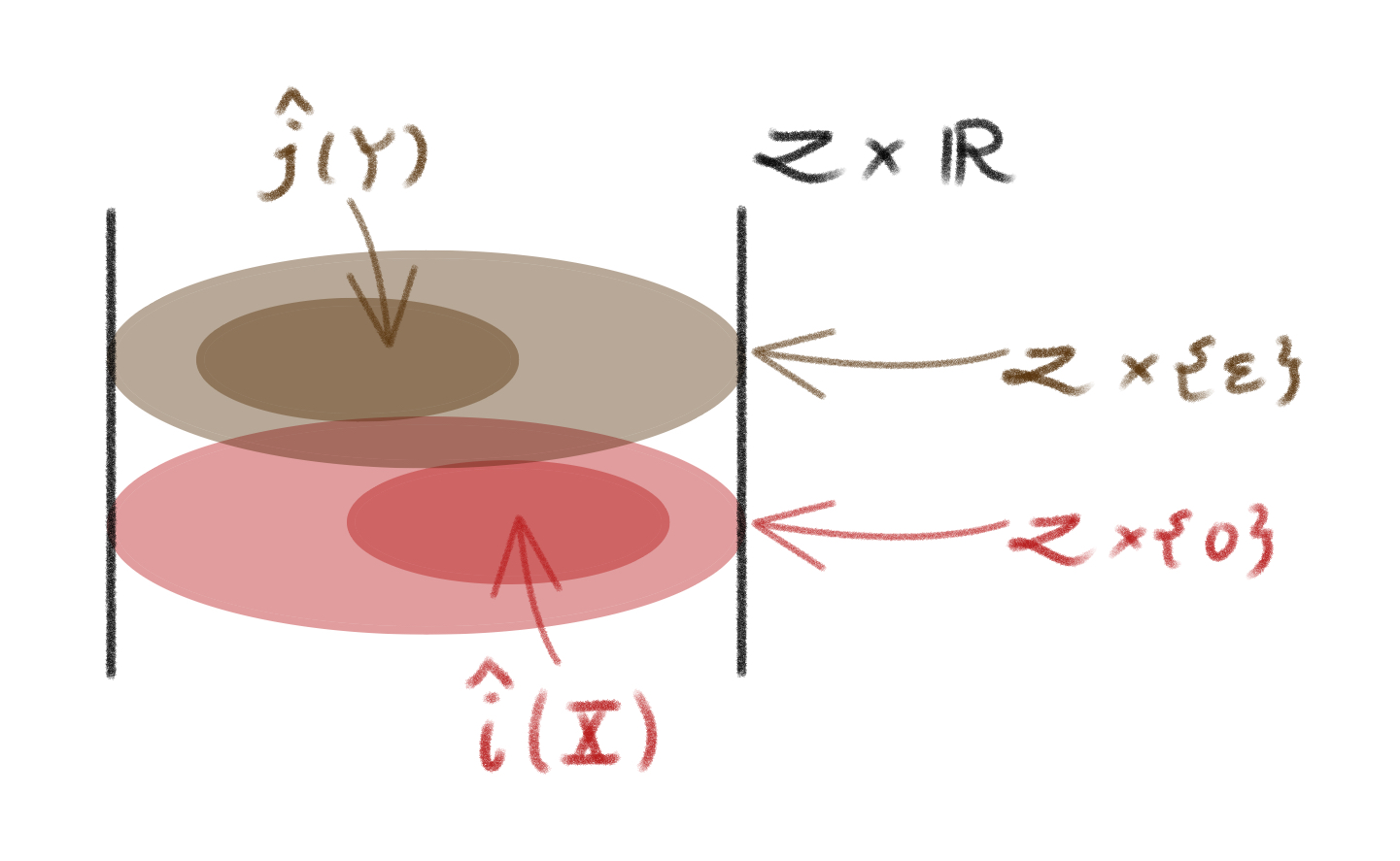
Figure 12.2: Construction of -
•
satisfies the triangle inequality. Fix and we claim that
Take , since we have metrics on and , say
in order to get the distance on , for , , we define
It is easy to check that this is a metric on and in this metric
Via the same approach of triangle inequality of , we can get the triangular inequality for as well.
12.3 The Topology of Isometry Class
Recall that we want to ensure that the Gromov-Hausdorff distance is a distance on the isometry classes of compact metric spaces. We have shown that it satisfies the triangle inequality. It is also obviously symmetric. Thus to check that it is a distance it remains to verify the following lemma.
Lemma 12.3.1.
Let and be compact metric spaces. Then
(We will prove this lemma later.)
Usually, computing the exact value of Gromov-Hausdorff distance is complicated and unnecessary. And mostly we are only interested in the topology induced by such metric, in particular in the notion of convergence.
Definition 12.3.2 (Gromov-Hausdorff Convergnce).
Let and be compact metric spaces, then we say converges to in the sense of Gromov-Hausdorff topology or if
Example 12.3.3.
One can check that
In order to verify this example, we only need to check
Example 12.3.4.
Let be a compact Riemannian manifold. Take a sequence . Denote (so that the distance in are multiplied by for each ). Then and hence . All the fine structures such as topology and curvature, etc. are forgotten. The only information left is the diameter. Therefore, we can say the Gromov-Hausdorff convergence is somehow a “weak” convergence.
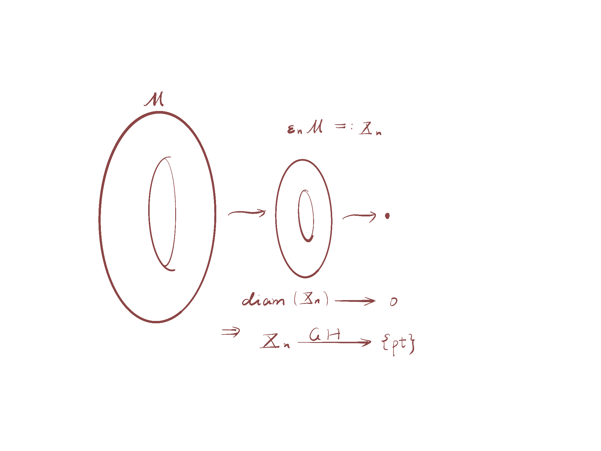
The above picture shows how the topological information is lost at the limit of the Gromov-Hausdorff convergence.
Example 12.3.5.
Consider with . Then as ,
Since
and
Thus, if , we have . This means if is -concave, then is -concave. Thus, at the limits, we know that is -concave, which just means concave.
Later, we will introduce the pointed-Gromov-Hausdorff convergence. And one can show that given a sequence of -concave function with and . We can conclude that pointwise converges to a -concave function .
In our case, consider , by the previous argument, we construct the following sequence of -concave functions . Since , we know that at , must be a concave function.
12.3.1 Gromov-Hausdorff Approximations
As we discussed in the example 12.3.4, even though the notion of the Gromov-Hausdorff convergence is “weak”, it is still useful because of the pre-compactness as we mentioned before (It is, in particular, useful to the class of manifolds with lower Ricci curvature or sectional curvature bound). In the example 12.3.4, where we start scaling down the Riemannian metric. We basically lose all the curvature bound (the curvature blows up). Thus, if we want to keep inside some class of lower curvature bound, we should be more careful and the Gromov-Hausdorff convergence will become more useful.
Now, we are going to list some more meaningful equivalent definitions that are going to help us to prove the lemma 12.3.1.
Definition 12.3.6 (-net).
Let be a metric space, a subset is called an -net in if , i.e.
Definition 12.3.7 (Totally Bounded).
A metric space is totally bounded if it has a finite -net for every .
Theorem 12.3.8.
A metric space is sequentially compact if and only if it is complete and totally bounded.
Definition 12.3.9 (-Gromov-Hausdorff Approximation).
Let and be metric spaces and let . Then is an -Gromov-Hausdorff approximation if
-
1.
For any ,
-
2.
is -dense in , i.e. for any , there exists such that . (Y = every point is not too far away from the image of .)
Remark 12.3.10.
In the definition 12.3.9 of -Gromov-Hausdorff approximation, there is no assumption on the continuity of the .
We will see the definition 12.3.9 is related to the Gromov-Hausdorff distance. But first of all, we want to list some of its properties
Proposition 12.3.11 (See page 258 in [BBI01]).
If , then there exists a -Gromov-Hausdorff approximation . Conversely, if is -Gromov-Hausdorff approximation, then
Proposition 12.3.12.
If is an -Gromov-Hausdorff approximation, then there exists which is a -Gromov-Hausdorff approximation.
Proof.
Suppose is an -Gromov-Hausdorff approximation. Take an -net in and set for each .
We claim that is an -nets in . Indeed, for any since is -dense in , there exists such that and we know that this for some . Thus,
Next, we can define as follows. For each , if for some , we take and for other , we can pick the with and set . In the case when for , we define (We just pick the one with a smaller index so that is well defined.). Then it is easy to see that is a -Gromov-Hausdorff approximation. Indeed. Let , then we know that there are such that and , thus and . Then
We still need to show is -dense in . Let , we can find such that . Take . By the definition of it is possible that for some such that . By the definition of -Gromov-Hausdorff approximation, we know that
Therefore,
Therefore, is also dense. ∎
Remark 12.3.13.
The above facts reflect that the definition of -Gromov-Hausdorff approximation is almost symmetric. And the function in the opposite direction is slightly worse.
The two properties above allow us to conclude the following corollaries.
Corollary 12.3.14.
Let be compact metric spaces. Then as if and only if there exists a sequence and there exists are -Gromov-Hausdorff approximation.
Corollary 12.3.15.
Every compact metric space is the limit of some sequence of finite metric spaces in the sense of Gromov-Hausdorff convergence.
Proof of Corollary 12.3.15.
Let be a compact metric space. Consider any sequence . Then for each , We can take
to be an -net in . Then the inclusion
is an -Gromov-Hausdorff approximation. Thus by the corollary 12.3.14. We can conclude that
∎
Now we can prove the lemma 12.3.1 which confirms the distance on the isometry classes of compact metric spaces.
Proof of Lemma 12.3.1.
Suppose , for , we know that there exists being -Gromov-Hausdorff approximation for some . And we also have the corresponding -Gromov-Hausdorff approximation.
Since is a compact metric space, it admits a countable dense subset say . We are going to use the diagonal argument to show that sub-converge to some which preserves the distances.
By the compactness of , the sequence sub-converges to some . As we define as we can easily show that is distance preserving, i.e.
This is because as (distance function is continuous)
We can extend to which is also distance preserving. This is because for each , by the compactness of and the fact that is compact, we can find a subsequence converges to . Moreover, is Cauchy which since
By the completeness of , we know that there exists such that . Thus we define . This extension is distance-preserving as well
Similarly, we get preserves the distance. However, to finish our proof, as we need to know that and are both surjective. This is not obvious and in fact can fail for noncompact spaces as the following example shows
Example 12.3.16.
Consider and such that . This is distance preserving but not surjective.
The following lemma shows that this can not happen if is compact.
Lemma 12.3.17.
Let be a compact metric space. If is distance preserving, then is onto.
Proof of lemma 12.3.17.
Suppose the lemma is not true. That is . Since is compact and Hausdorff, we know that the image is compact and closed. Let be an element in this open set (Notice that is closed). Thus there exists such that .
Let be a maximal -separated net in . The Finiteness of such net follows by the compactness of and is the maximal possible number of points in an -separated net. Now take , we know that since is distance preserving
which is again an -separated net. However, we know that
So that implies is also an -separated net but with elements, which contradicts the maximality of ∎
Now, we know that both and are distance preserving, both and are compact. Therefore and are also both distance preserving. Then by lemma 12.3.17, and are both surjective. Hence both and are onto and hence bijective then we can conclude
In particular, is a distance preserving bijective map. ∎
In the last lecture, we proved that the Gromov-Hausdorff distance is indeed a distance on the isometry classes of compact metric spaces. It is natural to wonder if it remains a metric on the isometry classes on complete metric spaces. It is easy to see that on this bigger class, is symmetric and satisfies the triangle inequality. However Lemma 12.3.1 fails for the class of metric spaces as the following example shows.
Example 12.3.18.
[By Kapovitch] We can construct an example that and are both complete metric spaces of finite diameter with but is not isometric to .
For each , we construct interval an such that and denote and the left and the right end of the interval. We construct by gluing for each together and all the for each together. It is not hard to see that is a complete metric space with a finite diameter. The only difference between the construction of from is that it has no interval . Notice that is not isometric to since an isometry must map an interval of length to an interval of length , which is impossible in our case.
To show that , we can show that for each . Let , we can construct an -Gromov-Hausdorff approximation in the following way. Consider the set , for each , is the identity map from to . Since has countably many elements, we can list them as and in particular we take . Then for each we have that . We can map to bijectively by an affine map sending endpoints to endpoints. Since it is easy to see that any such affine map is an -Gromov-Hausdorff approximation. Doing this for each an -Gromov-Hausdorff approximation .
Since this works for every we can conclude that .
We mentioned that in general Gromov-Hausdorff convergence is a rather weak convergence that is unable to preserve fine properties such as topology and curvature of the space. However, it becomes useful when we impose extra geometric restrictions on the metric spaces were are considering. In this section, we will see the class of compact spaces with an upper bound on diameter and a lower curvature bound is pre-compact in Gromov-Hausdorff topology.
Definition 12.3.19 (Inner/Intrinsic Metric Space).
Let be a metric space, it is called inner or intrinsic if for any ,
Definition 12.3.20 (Geodesic Metric Space).
An inner metric space is called geodesic if for any in the above definition the infimum is a minimum i.e. is realized by the length of a geodesic connecting and .
Example 12.3.21.
Inner metric space is not necessarily geodesic. For example, for and in (This space is not complete). The distance cannot be realized by any geodesic connecting and . However, the infimum exists and equals . The space in Example 12.3.18 is complete, inner but not geodesic.
Given any metric space , we can induce an inner metric space . Since we can define
Note however that might be equal to .
For example, we can define the inner distance on which is realized by the length of the geodesics lie in that connects points in .
Example 12.3.22.
Any Riemannian manifold is certainly an inner metric space. If it is complete, it is geodesic. This is followed by the Hopf-Rinow Theorem in Riemannian geometry.
Proposition 12.3.23.
Let be a complete metric space. Then it is geodesic if and only if it admits the mid-point property, i.e. for any , there exists an such that
Proof of Proposition 12.3.23.
-
•
“”: This is trivial. If is geodesic, then we can just pick the mid-point of the geodesic .
-
•
“”: Conversely, we want to use the mid-point property and the completeness assumption to produce a geodesics between and in . If the mid-point exists for any two points in , we can keep picking the mid-points again from the pairs and .
![[Uncaptioned image]](/html/2404.09792/assets/comparison_images/lec23image/IMG_2038.jpg)
Keep this procedure, we can define geodesics for diadic rational , i.e. get the position of the geodesics at a prior for each . This ensures us to define the geodesic on this dense set, say of numbers of . By the denseness of this set we can sub-sequentially approximate any using the sequence of these diadic times, i.e.
And because is complete, the Cauchy sequence
ensures the existence of such that . Hence we extend to entire . The resulting extension is easily seen to be a geodesic connecting to .
∎
Remark 12.3.24.
Completeness is necessary to define for all , not just for diadic rational . For example, has the midpoint property since for any the point is rational too.
But there are no geodesics between any two distinct points (because the cardinality from to an interval of rational numbers is different).
Proposition 12.3.25.
Suppose . Then if all have the mid-point property then so does . Therefore if all are geodesic then so is .
Proof of proposition 12.3.25.
Let be points in . we need to prove that there is a midpoint between them.
By the corollary 12.3.14, we can find and -Gromov-Hausdorff convergence . Therefore, for any , and . Now we can pick mid-point between . And it is easy to show sub-converges to a mid-point between and . ∎
12.3.2 The Pre-compactness Theorem
Definition 12.3.26 (Pre-compactness).
Given a metric space, a subspace is called pre-compact if its closure is compact. Equivalently, every sequence sub-converge to some limit point .
Definition 12.3.27 (Totally Bounded).
Recall that a metric space is totally bounded if, for every , it admits a finite -net.
We consider the following special family of metric spaces. Then, we are going to show this family of compact metric spaces is pre-compact under the Gromov-Hausdorff convergence.
Definition 12.3.28 (Uniformly Totally Bounded).
Let , a family of compact metric space is called uniformly totally bounded by , which is denoted as , if it is
-
•
Uniformly bounded diameter: for each ;
-
•
Uniformly totally bounded: and for each , there is a finite number such that any admits an -net with carnality less than or equal to .
where is called a covering function.
Theorem 12.3.29 (Precompcact Theorem of the Gromov-Hausdorff Convergence).
Let be a non-increasing covering function. Let . Then is pre-compact in the Gromov-Hausdorff topology. Namely, For any , there exists a convergent subsequence for some and admits the same covering function .
Sketch of the Proof of Theorem 12.3.29.
Fix an integer and let be a sequence. By the above, for any , we have find a -net in with elements.
Take a union of these for , which has elements in , say
Therefore, whenever we fix , we can have fixed number of points whose union is a finite metric space (finite subset of ). Recall that , so all the pairwise distance for the points in are , i.e. for any . Then by compactness of we can conclude subsequentially converge to a number for any . This is a limit metric on the set of finite points with cardinality less than or equal to .
Since
by the diagonal argument, we can get a metric on a countable set by passing to a sub-sequence. Here
and has elements for each . Then we take the metric completion of say and check that
∎
Recall that if we fix , and consider the following family of closed Riemannian manifolds:
then by the Bishop-Gromov volume comparison theorem, for any there exists such that for any , admits an -net with elements. And thus we have a natural corollary by the theorem 12.3.29.
Corollary 12.3.30.
is precompact in Gromov-Hausdorff topology. Being pre-compact means every sequence
admits a convergent sub-sequence in Gromov-Hausdorff topology. But the limit may not be smooth or even a manifold.
Fact 12.3.31.
If is precompact then any is precompact too.
An easy corollary from this fact is:
Corollary 12.3.32.
The following family of closed Riemannian manifolds
is also precompact in the Gromov-Hausdorff topology.
Proof.
Because implies . ∎
Chapter 13 Alexandrov Spaces
13.1 Introduction
Recall that precompact means every sequence has a convergent subsequence. And it is natural to ask what the limit looks like, of sub-sequences in Corollary 12.3.32. To answer this question, we need to study Alexandrov geometry.
Definition 13.1.1 (Alexandrov Space).
Let be a complete geodesic metric space is called Alexandrov of curvature if the following four-point condition in the Toponogov comparison holds. Namely, for any four points , we have
if such comparison triangles exist.
Therefore, by the Toponogov comparison, with this definition, every complete Riemannian manifold with is an Alexandrov space of curvature .
Remark 13.1.2.
More generally, one can consider inner metric instead of geodesic Alexandrov spaces. But in finite dimensions the two notions are equivalent.
Alexandrov’s condition is preserved under the Gromov-Hausdorff convergence.
Proposition 13.1.3.
Suppose where are Alexandrov spaces of curvature , then is also an Alexandrov space of curvature .
Proof of Proposition 13.1.3.
Firstly, we just pick . Since , then by the corollary 12.3.14, we have a sequence and the corresponding -approximation for each . Fix , since is dense in for each , we can pick the corresponding in such that
Moreover, since are Alexandrov of curvature , the four-points comparison holds for each group of , say
Since the Gromov-Hausdorff convergence implies the convergence of the geodesics 12.3.23, say
Then, by the cosine law, the sequence of angles in the model space will certainly converges.
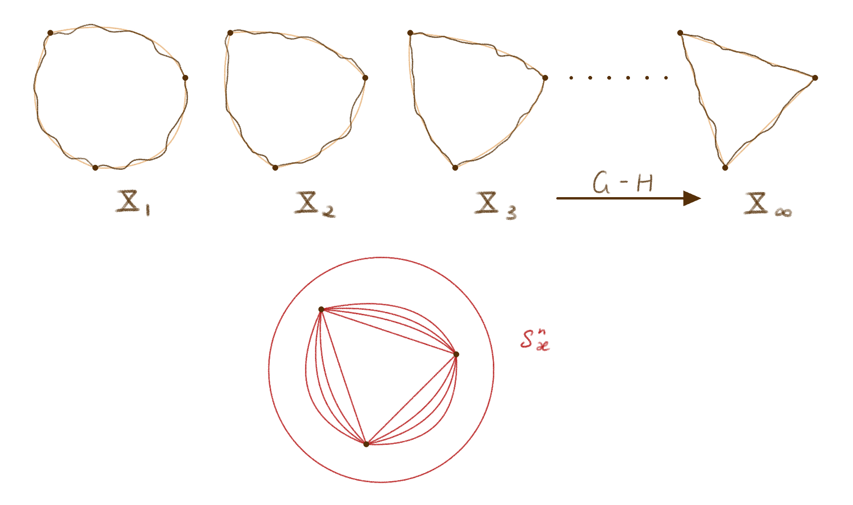
Therefore, the convergence of angles implies
Then we can conclude that is also an Alexandrov space of curvature . ∎
Now we can answer our question rises from the corollary 12.3.32, the sub-sequential limits of the manifolds with are Alexandrov spaces of curvature .
13.2 Examples
So far we have introduced the notion and the motivition of Alexandrov spaces. In words, the study of Alexandrov geometry is the study of the Toponogov comparison theorem in the context of geodesic metric spaces. Alexandrov spaces have many properties similar to manifolds. We are going to list some of them.
Example 13.2.1.
Let be compact manifolds of where . Consider a connected compact Lie group acting by isometries . As every compact Lie group has a bi-invariant Riemannian metric so that . Take any , take where . The space still has . And diagonally as isometries. This action is free and isometric. Take , which is diffeomorphic to with different metrics, and orbits of are shrunk. We have a Riemannian submersion . By theorem 6.2.1 it holds that for any . In particular, it is an Alexandrov space of .
Finally,
Therefore, we can show that is an Alexandrov space of curvature .
The construction in the example 13.2.1 allows us to produce Alexandrov spaces that are not manifolds. Below is a more explicit example of such non-manifold Alexandrov space.
Example 13.2.2.
Notice that . So is an Alexandrov space of curvature . Consider , which is an isometric action
By the last example 13.2.1, we know that is an Alexandrov space of curvature . Indeed the cone of which is not a manifold. Intuitively, and the cone structure comes from . And this example is non-compact.
Example 13.2.3.
Let be complete with . Suppose is convex. Then the level set with respect to the intrinsic metric is an Alexandrov space of curvature . For a smooth this follows by the Gauss formula which implies that is a smooth manifold of . The general case follows by approximation.
In particular, for any convex body , its boundary is an Alexandrov space of curvature . In particular, the boundaries of the convex body having infinite many corners are also Alexandrov spaces of . . To see why this is true, there exits a convex function such that . The function can be smoothed out by taking convolution with smooth kernels. This gives point-wise and all are smooth and convex. We claim that in intrinsic metrics. Therefore, is also an Alexandrov space of curvature .

To show this, notice that -point-wise implies in the Hausdorff sense as subsets of . However showing convergence in intrinsic metrics is less obvious, even in low dimensions. For example, for convex function on and smooth convex functions point-wise converge to . Then over the closed interval ,
is not an even trivial convergence.

To show this convergence in intrinsic metric is true, we have to use Sharafutdinov retraction. Since ,
we have the Sharafutdinov retraction , which is a -Lipschitz retraction from .
We consider the restriction which is also a surjective -Lipschitz map. And similarly we get another Sharafutdinov retraction which is also surjective -Lipschitz and its restriction is also surjective -Lipschitz. Since and can be chosen to be norms on , different level sets are homeomorphic to each other. The end result is that we have
Because they are all proportional to each other, we can just write
Roughly speaking, we have the almost -Lipschitz functions between and for both directions.
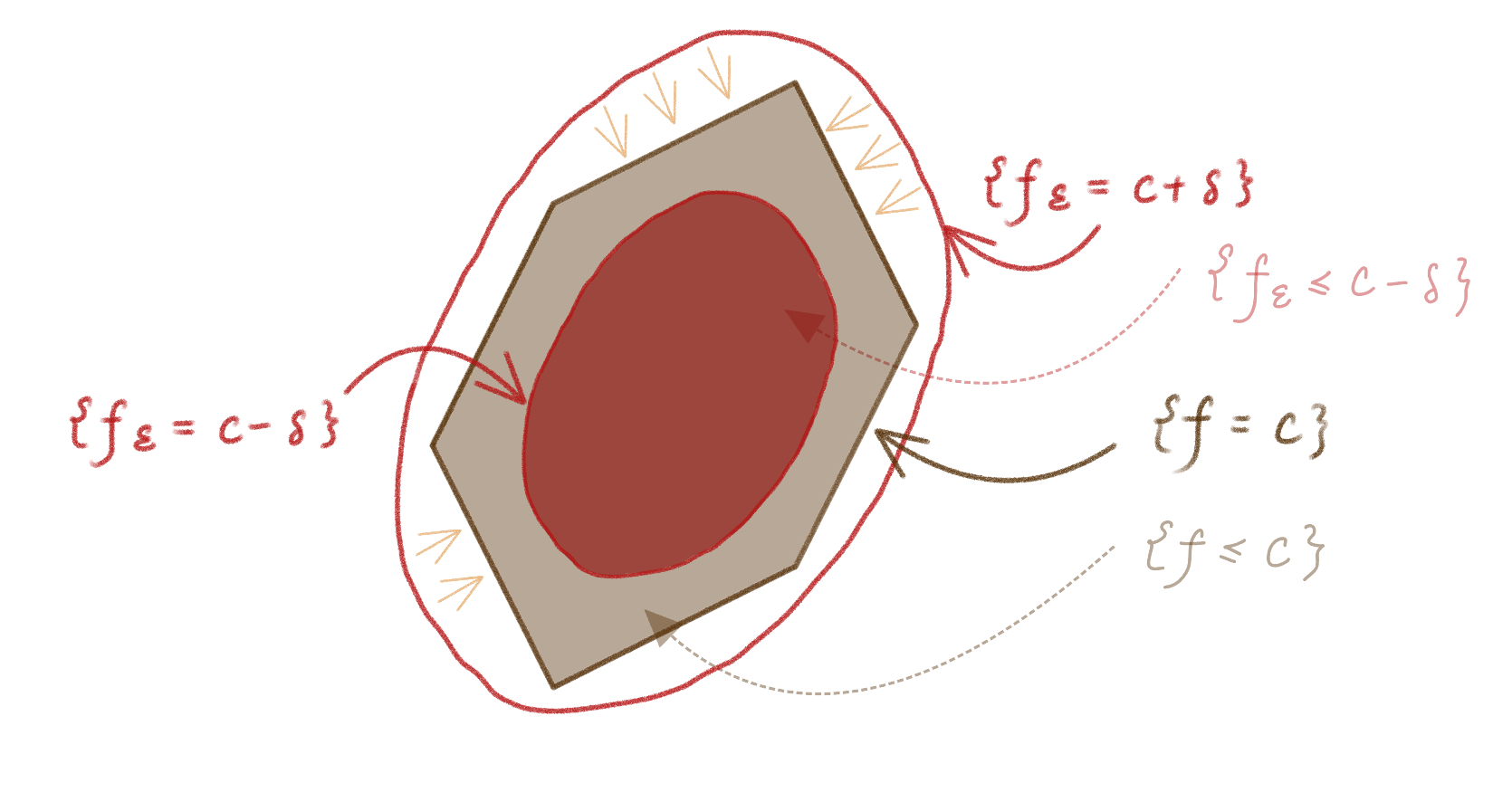
Take the composition of the two maps,
is surjective -Lipschitz. And as , the composition will converge to some map which is also surjective -Lipschitz. Then by the following lemma (The proof is left as an exercise, which can also be found in [BBI01])
Lemma 13.2.4.
Let be a compact metric space. Then if is surjective -Lipschitz, then is an isometry.
By passing to a limit as we can conclude that and are -Gromov-Hausdorff approximations.
13.3 Pointed-Gromov-Hausdorff Convergence
Let , be proper metric spaces, i.e. closed balls are compact. Here and are points in the space. For example, complete Riemannian manifolds are proper metric spaces.
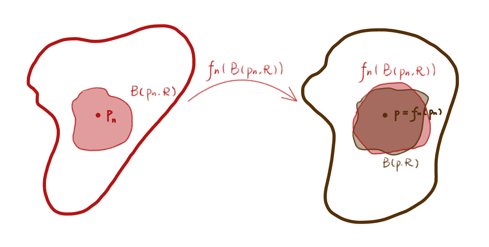
Definition 13.3.1 (Pointed-Gromov-Hausdorff Convergence).
Let , be proper metric spaces. The convergence
is called a pointed-Gromov-Hausdorff convergence if such that and fixed, is an -Gromov-Hausdorff approximation onto where as .
Example 13.3.2.
If is a Riemannian manifold. Let and a sequence. Then
where is the point corresponding to in . And means the rescaled manifolds of by factor . Thus any ball of radius in becomes a unit ball in . Finally, the nontrivial Riemannian metric will become flat at the limit of the pointed Gromov-Hausdorff convergence.
The phenomenon in this example 13.3.2 can be generalized to Alexandrov spaces with a lower curvature bound. The generalization is constructed in the next lecture.
Let be an Alexandrov space of curvature . Moreover, we assume has a finite Hausdorff dimension.
Notes 13.3.3.
Remember that is denoted as the -dimensional Hausdorff measure. And for some space
for some integer . Furthermore , the topological dimension of . We will refer to as dimension of and will denote it by .
And behaves like volume on manifolds. Here are some properties of the Hausdorff measure and the Hausdorff dimensions we would like to mention:
-
•
Moreover, is continuous with respect to the Gromov-Hausdorff topology. Namely, suppose we have a sequence of Alexandrov spaces of curvature and . If
to some Alexandrov space of curvature . Then we can conclude that
-
–
;
-
–
and if , then
-
–
-
•
The Bishop-Gromov comparison holds for . Proving this is similar to the Bishop-Gromov comparison for . This theorem is generalized to the Alexandrov spaces.
13.4 Properties
We can summarize those properties as the followings. Fix , an -dimensional Alexandrov space of curvature .
-
•
We can define angles in using the comparison angle in the model space . Namely, for two geodesics starting at we can define the angle between and at as the limits of the angle in the model space:
-
•
Other versions of Toponogov comparison theorem hold;
-
•
Globalization theorem holds: if Toponogov holds locally then it holds globally.
-
•
We can define tangent space for Alexandrov space of curvature . More detailed construction of the tangent space can be found in the section 13.5.
-
•
If , then is an integer and the -th Hausdorff measure behaves like the volume on manifolds. In particular, the Bishop-Gromov volume comparison holds. Absolute volume comparison holds as well.
-
•
the volume function on Alexandrov space is continuous concerning the Gromov-Hausdorff convergence. Let be a sequence of -dimensional Alexandrov space of curvature with . Then the Gromov-Hausdorff limit of the sequence is again an Alexandrov space of curvature , , . And
and in particular, if , the sequence of volumes converges to .
Example 13.4.1 (Example of Volume Collapsing).
Notice that . Consider the Hopf action : Since we can consider . And as unit complex number. So that for we can write any complex number as . This action is free and isometric. Now we can construct our volume collapsing example. Let be the circle of length . Consider , for each , this space has nonnegative sectional curvature. Let , then
because . Hence we have the volume collapsing.
-
•
Let be an Alexandrov space of curvature . Let be a semi-concave function. Fix , we can have the gradient defined in the same way as we did for manifolds. So the gradient flow exists and has the same contraction properties as manifolds for the same reason.
-
•
The first variation formula holds for Alexandrov spaces. Let be an Alexandrov space of curvature . Let be an -concave function. The its gradient flow is -Lipschitz. Toponogov condition implies there are many semi-concave functions in Alexandrov spaces.
Example 13.4.2.
Let be an Alexandrov space of curvature . And a closed subset. Then is -concave just like for Riemannian manifolds of nonnegative sectional curvature.
-
•
The splitting theorem holds. The same proof works. Let be an Alexandrov space of curvature . If has a line then
where is also an Alexandrov space of .
Remember that we want to generalize the phenomenon of example 13.3.2 of Riemannian manifolds to Alexandrov spaces with lower curvature bound. That motivates us to define the notion of tangent spaces for Alexandrov spaces.
13.5 Tangent Spaces and Cones
We can also generalize the concept of tangent space to Alexandrov spaces. Given a point in an Alexandrov space. We can look at geodesic directions starting at , say , and take a metric completion denoted as with respect to angle metric. We call the space of directions at . It is an analogue of unit sphere in if is a Riemannian manifold. Now the tangent space of is defined as which is the Euclidean cone over the space .
Recall that the Euclidean cone is constructed as the following. If is a metric space then its Euclidean cone is defined as .
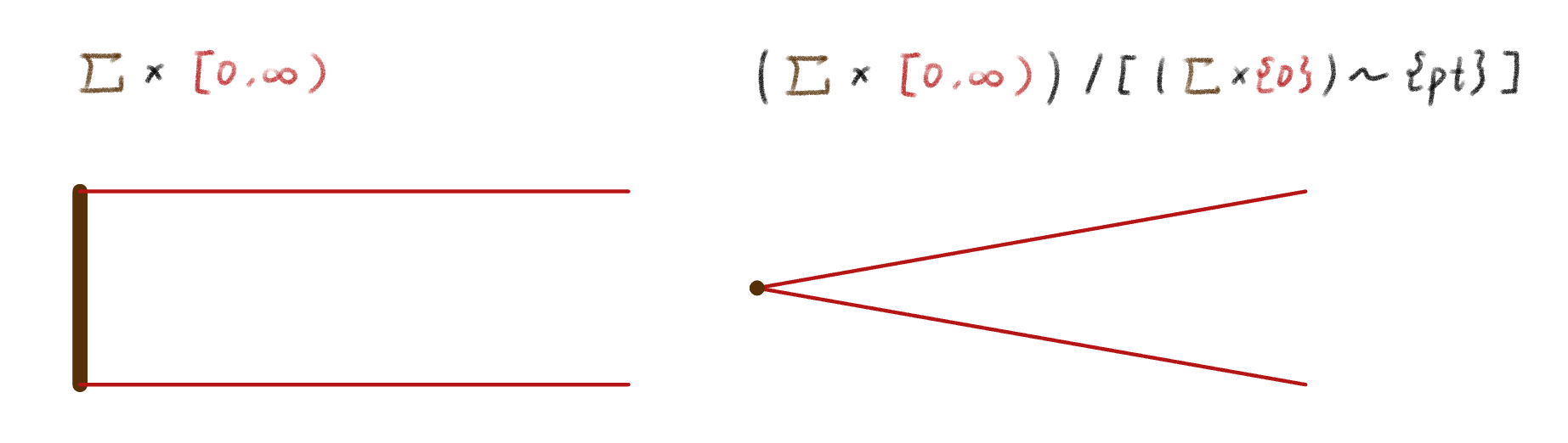
is again a metric space as well and we can define the distance function .
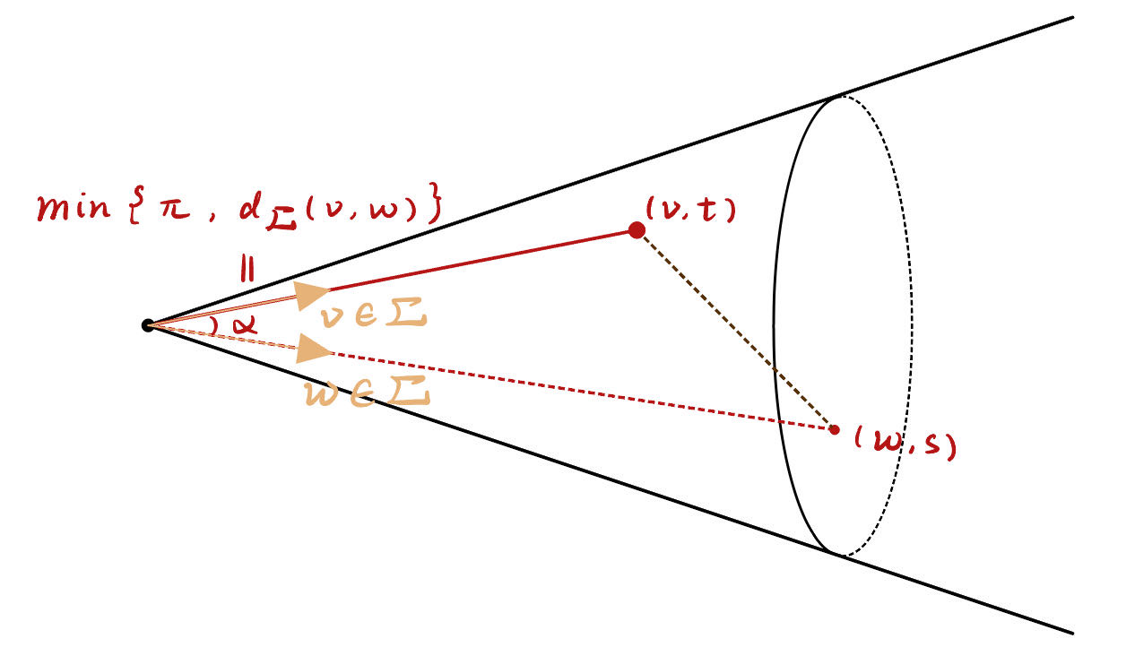
For each and ,
where . We should consider as the angular metric.
Definition 13.5.1 (Tangent Space of Alexandrov Space).
Let be a -dimensional Alexandrov space. By our construction above, the tangent space, denoted by , of at is defined as
is again a metric space equipped with the metric , which also has been constructed already.
Theorem 13.5.2 (See [AKP22]).
is Alexandrov of curvature if and only if is Alexandrov of curvature .
Now we can generalize the example 13.3.2 to the Alexandrov space with a lower curvature bound.
Theorem 13.5.3.
Let be a finite-dimensional Alexandrov space of curvature , we have the following pointed Gromov-Hausdorff convergence
where is the cone point.
Corollary 13.5.4.
Moreover, if the curvature of is , then the curvature of is just like the situation for manifolds. Therefore, is of the curvature at the Gromov-Hausdorff limit, which means is an Alexandrov space of curvature . By Theorem 13.5.2 that implies that has curvature .
13.6 More Examples
Example 13.6.1.
In particular, if is a Riemannian manifold. Then ,
Fact 13.6.2.
We would like to mention the fact that if is an -dimensional Alexandrov space, then for almost all with respect to .
Example 13.6.3.
If is a complete Riemannian manifold of , then it is an Alexandrov space of curvature .
Example 13.6.4.
Let be an Alexandrov space of curvature . And is a compact Lie group and by isometries. Then gives us again an Alexandrov space of curvature . Many singular examples can be produced in this way. More generally if is an Alexandrov space of curvature and is a submetry then is also an Alexandrov space of curvature .
Example 13.6.5.
If is an Alexandrov space of curvature and a closed convex subset. Then is also an Alexandrov space of curvature . In particular, any convex body in is an Alexandrov space of curvature .
Example 13.6.6.
Let be a Riemannian manifold of and let be a convex function. Then is an Alexandrov space of curvature .
Conjecture 13.6.7.
The statement of the example 13.6.6 is unknown but widely expected to be true if we weaken the assumption that the ambient space is a Riemannian manifold to an Alexandrov space.
Chapter 14 Grove-Peterson Homotopy Type Theorem
14.1 Preliminaries
The following fact 14.1.3 explains why the Alexandrov space of lower curvature bound is better in Gromov-Hausdorff convergence.
Notation 14.1.1.
We denote the family of the Alexandrov spaces of curvature as .
Notation 14.1.2.
Fix . We denote
the family of Alexandrov spaces with bounded dimension and diameter. And in addition, we denote
Fact 14.1.3.
and are both compact subsets of in the Gromov-Hausdorff topology.
Remark 14.1.4.
The spaces and are bigger comparing with and
Remark 14.1.5.
Remark 14.1.6.
There is a similar metric measure generalization to spaces, i.e. the family of Riemannian manifolds of and bounded dimension. But we are not going to discuss that in this course.
In this section, we want to prove the following theorem.
Theorem 14.1.7 (Grove-Peterson).
Fix , and . Consider the following family of -dimensional Riemannian manifolds.
Then contains only finitely many homotopy types of manifolds. That is, up to homotopy equivalence, it has only finitely many elements.
Note that . And it is also true that contains finitely many homotopy types, In fact, also homeomorphism types. This follows from the Stability Theorem of Perelman.
The scheme of the proof of the Grove-Peterson theorem 14.1.7 is an argument by contradiction:
Sketch Proof of Theorem 14.1.7.
Suppose the theorem is not true. That is, we have a sequence of such that , is not homotopy equivalent to . Then by compactness, we have a subsequence
where . The reason for being dimensional is that we have the lower volume bound for each so there is no volume collapse at the limit. Next, we want to try to show that for large all are homotopically equivalent to and hence contradiction.
It requires some work to show for large all are homotopically equivalent to . ∎
14.2 Grove-Bishop-Gromov Volume Comparison
To prove the theorem 14.1.7 rigorously, we need a generalization of the Bishop-Gromov volume comparison theorem.
Theorem 14.2.1 (Grove-Bishop-Gromov Volume Comparison).
Let be a complete Riemannian manifold with . And the simply connected model space of . Let be a compact set and the -neighborhood of . Let . Then the quantity
| (14.1) |
is non-increasing in . The classical Bishop-Gromov volume comparison now becomes the special case when . This result is true for any compact subset .
The idea is that we first prove the result for any finite set . And if this is true, we can take denser and denser finite subsets of points for general . Then we can apply the theorem to the denser set and pass to the limit of these denser and denser sets.
14.2.1 Voronoi Cells Construction
As we mentioned, we first consider the case when is a finite set. An important idea here is to construct Voronoi cells for and decompose the manifolds into pieces having nice geometric features.
Definition 14.2.2 (Voronoi Cell).
Given a finite subset , we can define corresponding Voronoi cell which is denoted as
It is clear that .
Here we list two important facts of the Voronoi cells.
Fact 14.2.3.
If then and are half-spaces bounded by the hyperplane perpendicular to and passing through its middle. Therefore if then each Voronoi cell is an intersection of several half spaces. In particular it is convex.
Fact 14.2.4.
Given a finite subset . we can show . Thus up to measure , we can think of as a disjoint collection of subsets.

In Riemannian geometry, we have the local uniqueness of geodesics if the initial condition is given. However, in a general geodesic metric space, this property may fail since two geodesics with the same initial condition may split at some point (Example 14.2.5). We will show that the property that geodesics do not split holds in Alexandrov spaces with lower curvature bound.
Example 14.2.5.
Let , i.e. for , . Let , , . Then the geodesic segment and (See Figure 14.2). Notice that , which is an interval. In this example, two geodesics branch at .

Definition 14.2.6 (Non-Branching Subset (From [RS12])).
Two geodesics are branching there exist such that but . A metric space is called non-branching if there are no branching geodesics.
Lemma 14.2.7 (Non-Branching Property of Alexandrov Space).
is non-branching.
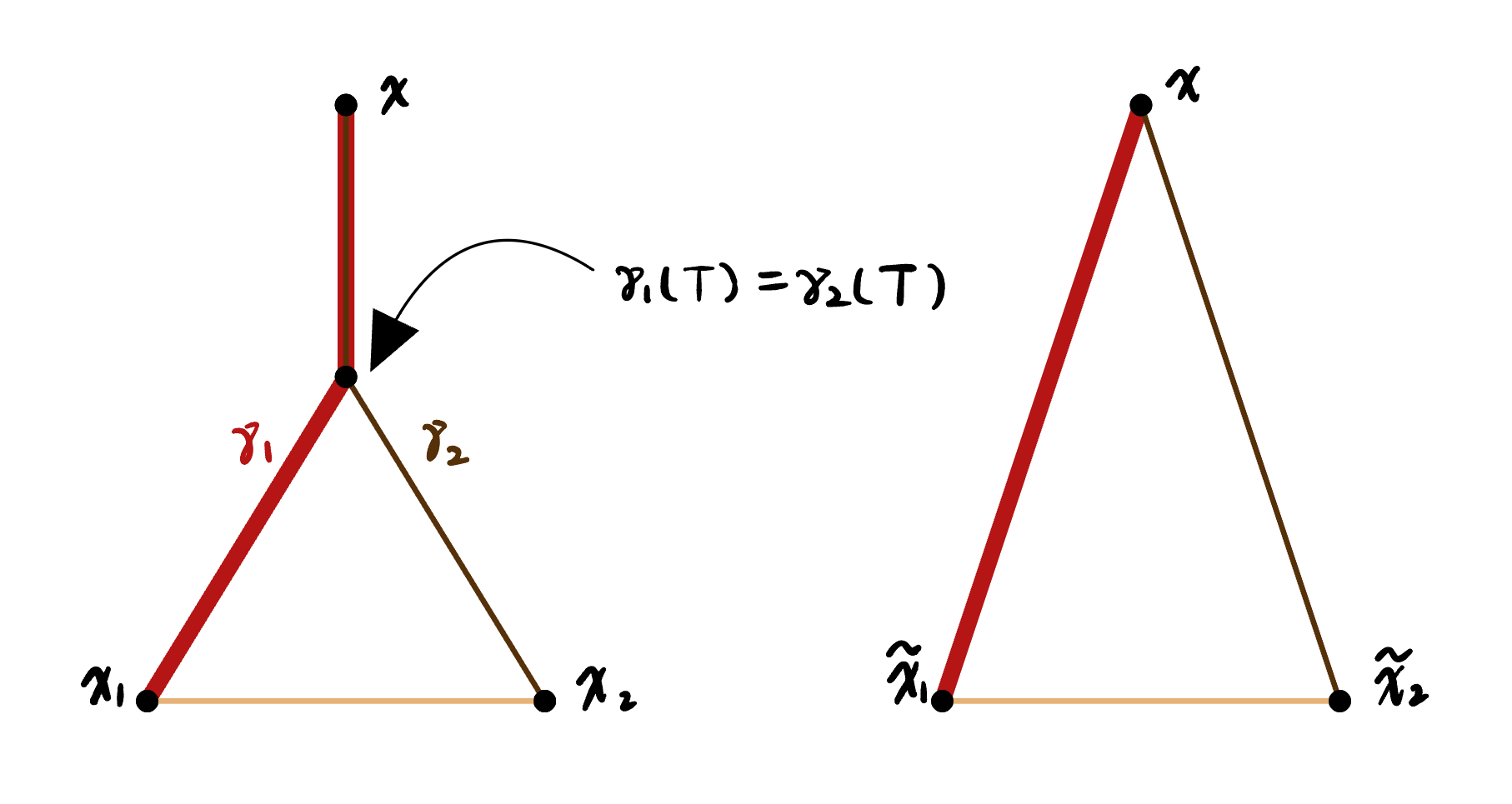
Proof.
Let be two geodesic segments such that for some , We denote
We can use a contradiction argument to show . Since , we know that , without lost of generality, we suppose for all . Especially, we denote , and . We can see from Figure 14.3 such that the angle for the triangle (See Definition 2.1.5 and Notation 2.1.8). By the definition of and the equivalent statements of Toponogov comparisons. We know the Toponogov angle comparison holds in . Therefore, this means the comparison angle in the model space is zero. However, since are three distinct points, then it is impossible to have . Contradiction! ∎
Lemma 14.2.9.
Given a finite subset of an Alexandrov space of curvature , say . Then is star-shaped with respect to , i.e. for any , the geodesic segment .
If we parametrize using such that , if for some , then and . Furthermore, if , we must have .
Proof of Lemma 14.2.9.
Denote and the distance function of the alexandrov space and consider the unit speed geodesic . In particular, we set , and thus
decreasing with speed , i.e. . Let . We know that is an -Lipschitz function and hence its right derivative exists a.e. satisfies
the function decreases with the speed at most . Thus we know for any , we have
Therefore we can conclude that
for all . Thus we have
for all .
Now if for some , this means the following inequalities
are all equalities. This implies , which means .

Next we claim that if then . Suppose this is not true, i.e. for some . By above this implies , namely, and . By our assumption, we also know that . This makes the length of the hinge equals to and thus both and are geodesics from to . However, we notice that this means the geodesics and branching at as in Figure 14.4, which is impossible by the above Lemma 14.2.7. ∎
14.2.2 Volume Comparison for Finite Set
In this section, we claim that the theorem 14.2.1 holds in the case when is finite. Namely, we need to show in 14.1 is non-increasing.
By the fact 14.2.4, we can essentially think of as a disjoint union decomposed by Voronoi sets upto measure , i.e.
That implies that
Therefore, it is enough to prove that
is non-increasing for each .
Now, we need to define our cut function. Fix a unit vector , we denote the cut-time of the pair . Then, for the unit speed geodesic
and define the function
Thus it is always true that . Then we proceed as in the proof of the original Bishop-Gromov comparison. For the geodesic , we can consider parallel unit orthonormal vector fields along perpendicular to . Thus we can get the Jacobi fields along such that for each ,
Then we can define
in basis. Now we redefine using . Namely,
Next, we just proceed the proof as in Bishop-Gromov comparsion. Consider the quantity , where is the corresponding function in the model space (). Notice the quantity is non-increasing because we can apply the same proof to the star-shaped region . Therefore, we get
Meanwhile, as in Bishop-Gromov comparison, this is divided by
Thus we obtain the monotonicity by the same argument as in the original proof of Bishop-Gromov.
14.2.3 Approximation Arguments by Finite Sets
As we mentioned in the beginning, we can pick denser and denser subsets so that the theorem 14.2.1 is also true. For compact set , we can pick a sequence of finite sets such that the Hausdorff distance
as . This is possible since for any , we can find a finite -net in .
And thus, point-wisely,
Hence, we have the point-wise convergence,
Thus, we can generalize the theorem 14.2.1 from finite set to compact set since monotonicity is preserved under point-wise convergence.
14.3 -Critical Points Theory
From our new volume comparison theorem 14.2.1, we have the following corollary which particularly estimates the volume of small annuli in a sphere. This corollary is important for proving the theorem 14.3.5. And this theorem is essential for the Grove-Peterson theorem.
14.3.1 Volume Estimates for Small Annulus.
Corollary 14.3.1.
Let be a closed subset. And denote the annulus in with respect to the set , i.e.
Then for sufficiently small it holds that
where is some universal constant depends on .
Proof of Corollary 14.3.1.
This corollary is easily followed by the Bishop-Gromov volume comparison. According to the Bishop-Gromov’s conparison, if , then
Notice the LHS of the inequality above,
Similar things can be applied to the RHS. Therefore,
If , , , . Then is just the -neighborhood of the equator of .
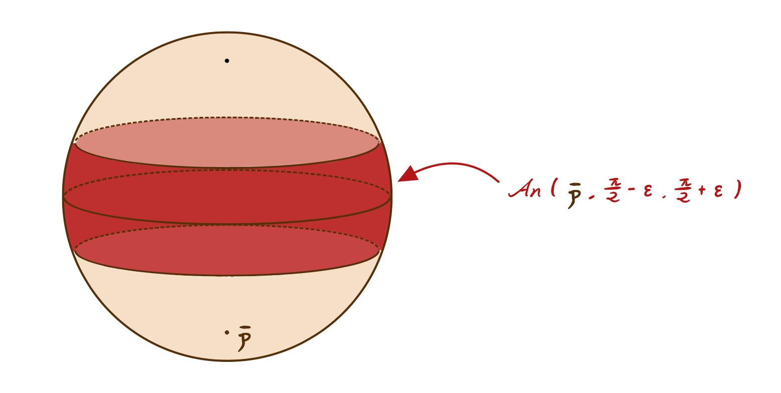
Therefore, the volume of the -neighborhood is . Therefore, it follows that
∎
14.3.2 Introduction to -Critical Points
We will need the following relaxation of the notion of a critical point of a distance function.
Definition 14.3.2 (-Critical Point).
Let be a compact Riemannian manifold. Let and let . Then is called -critical for , if
In particular, is just a critical point for when as we commonly defined.
For general semiconcave function on , let and let , we say is -critical at if for all unit . Similarly, is -regular at is for all unit .
Now by the first variation formula, consider all the shortest geodesics starting from to and fix a unit vector at . Denote
so . Then we can see that is -critical if

This gives us the following equivalent definition of an -critical point.
Definition 14.3.3 (Equivalent Definition of -Critical Point).
Let be a compact Riemannian manifold. Let and let . Then is -critical for if for any -unit vector at , there exists such that
The following example shows that if there is no lower volume bound mutually -critical points can be very close to each other.
Example 14.3.4.
Consider a sphere of radius , then any pairs of points and that are opposite to each other are also -critical to each other.
After a brief discussion of -critical points, we would like to use the following theorem to show how -critical points are distributed in Riemannian manifolds. Indeed, we can show that if two points are mutually -critical to each other, then these points cannot be too close to each other.
Theorem 14.3.5.
Fix , and . Consider the family of Riemannian manifolds
Then there exists and such that if are mutually -critical to each other, then
Proof of Theorem 14.3.5.
Assume for simplicity and sufficiently small and take . Suppose are mutually -critical to each other and . We want to show that this implies the volume of the manifolds is small, i.e.
which leads to a contradiction.
Since and , . By Bishop-Gromov volume comparison,
| (14.2) |
We want to estimate the volume of . Fix . Then we have
![[Uncaptioned image]](/html/2404.09792/assets/comparison_images/lec25image/IMG_2056.jpg)
Connecting using shortest geodesics (May not be unique). We take , and and denote be the corresponding angles in the model space . Moreover, we denote the corresponding points of in the model space by requiring
Therefore, by the trigonometry in the Euclidean space, we have
for some constant . By Toponogov comparison, we have
On the other hand, since ,
Therefore, we can conclude that
then
Let be the unit vector at along the geodesic then by the inequalities above, we have
Recall the corollary 14.3.1, there exists such that for any closed subset , we have
In our case, since we can think of unit vectors as elements of a unit sphere and have angular distance, we have
where
Recall by Rauch or Toponogov theorem, consider
and we choose a set inside cut-locus. Then on , is -Lipschitz. Therefore, it does not increase volume, i.e.
But since . Also, since , we can express each elements in polar coordinates, i.e. where is an unit vector. And , . Since ,
And again since is -Lipschitz on this set. Then
therefore, together with the inequality 14.2, we have
Finally, if is small enough so that the of the above inequality is , we can get the contradiction. Namely, if we take
then are mutually -critical and which is just the contradiction. ∎
Let’s use an example to understand the contradiction in this theorem 14.3.5 better.
Example 14.3.6.
Let . Let be a fixed number so that . Obviously, the volume of is small if is small. Let be opposite points in which are certainly mutually -critical to each other. The distance of and is .

Same as what we did in the proof of the theorem 14.3.5, we pick such that , then what happens is that for ,
and this forces the volume of to be uniformly small.
14.4 Homotopies and Diagonal
Notation 14.4.1.
We define the notation for the distance function for the product of two spaces, i.e. for metric space and , we can define and denote the distance function for as
In case is equal to with a metric induced by a Riemannian metric on the distance is induced by the Riemannian metric . Also, note that if satisfies then
Lemma 14.4.2.
Let be a complete Riemannian manifold. Consider the product with the product metric.
Take the diagonal
Then, for any , we have
Proof.
Let , we firstly notice that for any point , we have
On the other hand, we can take the shortest geodesic from to in where .
And we pick the midpoint , so that
Thus,
This means this point admits the shortest distance from the diagonal to . Indeed, we can construct the geodesic from to as where such that
∎
Remark 14.4.3.
More generally, this corollary can be extended to any geodesic metric space .
Proposition 14.4.4.
Consider such that is -regular to or is regular to ( and cannot be mutually -critical to each other.)
Let .
Then
Proof of Proposition14.4.4.
Without the loss of generality, we assume being -regular for , then such that
| (14.3) |
Thus, if we take , . we have
Similarly for being -regular for , we take .
In either case, we can see that
∎
Combining the proposition 14.4.4 with the previous theorem 14.3.5, we can conclude the following corollary.
Corollary 14.4.5.
Let . Let , be given by Theorem 14.3.5,
then is -regular on the -neighborhood of the diagonal minus the diagonal, i.e.
and on .
This corollary allows us to construct a smooth unit gradient-like vector field on such that for every and , we have
Note that near the diagonal , namely, inside the normal injective radius, we can just take which has length . This is the region where the normal exponential map is diffeomorphism, we can just take unique shortest geodesics in the image of the exponential map. Then along integral curves of , increases with speed .
Along integral curves of , decreases with speed at least , that means if we have a point and the backward flow of , then
which means the flow hits the diagonal. Therefore, we can conclude that is a deformation retraction from the neighborhood to and length of all integral curves starting at satisfies
Remember that and and . Thus we can construct a new curve , such that
The family of curves , whose length is continuous with respect to the distance of . Given any pairs such that , we have
Corollary 14.4.6.
Under the assumptions of Corollary 14.4.5 there is a continuous map such that for any it holds that
Corollary 14.4.7.
For and , as above, a metric space, are -close, i.e. for any . Then we can conclude that (homotopic).
Proof of Corollary 14.4.7.
Take . It is a curve connecting and which is continuous in both and . Thus it is homotopy from to . ∎
Remark 14.4.8.
In the corollary 14.4.7, . More precisely,
We are going to use that to prove the Grove-Peterson theorem 14.1.7. We need the following lemma
Lemma 14.4.9.
Let and be small, i.e. 111If then needs to be sufficiently small in order for this inequality to be satisfied Let be a -net in . If, by maximality . Then the multiplicity of this cover is controlled by a universal constant . Namely, for any , by the maximality, we know there is a constant such that
We can always say this .
Proof of Lemma 14.4.9.
If , then for each pairs of we have . We can rescale by , i.e. so that . Then in , for any , we have
Therefore, by Bishop-Gromov volume comparison, the number of such s is . Indeed, we know that there is a constant such that
Notice that since ,
Thus,
On the other hand, because . We can conclude that
Therefore, we have .
∎
14.5 The Proof of the Grove-Peterson Theorem
In this section, we are going to finish the proof of the theorem by Grove-Peterson on Finite Homotopy Types 14.1.7
Suppose the theorem is not true. That is, if the class has infinitely many homotopy types of manifolds, i.e. there are a sequence of manifolds that are not pair-wisely homotopy equivalent.
By our conclusion on the pre-compactness 12.3.32, by passing to a subsequence we can assume that (See Notation 14.1.2) by passing to a subsequence.
Let and be given by Theorem 14.3.5 and Lemma 14.4.9. Take And consider be the maximal -separated net in such that .
By Corollary 12.3.14, we know that there is a sequence and there exists the -Gromov-Hausdorff approximations. Recall that from the Definition 12.3.9, this implies is -dense in . This means, for each , we can have the corresponding in such that
for each . Indeed we can show that is an -nets for . Indeed, for each , , thus there exists such that . Since is an -Gromov-Hausdorff approximation, we can find such that . We claim that . To show this, remember that we have
following from the definition of -Gromov-Hausdorff approximation. This implies that
Since we have , we can take sufficiently small such that
We want to extend from the set to the entire continuously in a controlled way (we are going to explain what we mean by “a controlled way” later).
14.5.1 Center of Mass Construction
The idea of the extension is to use the center of mass construction.
In the case when , take the partition of unity of on subordinates to our cover . That is
-
•
For each , ;
-
•
And when , ;
-
•
;
-
•
over .
By the Lemma 14.4.9, for each , then the number of is at most of these. And now we only look at those points. By considering as a number, we can take the extension, still denoted by , as a convex linear combination of ’s, i.e.
, which provides us a point in a simplex spanned by . Our extension is continuous and -Gromov-Hausdorff approximation.
We want to generalize this to our situation when is not necessarily . Let’s initially assume a smooth manifold. Eventually, instead of a map , we will do the center of mass construction of for large222The center of mass construction can be made to work in general Alexandrov spaces but that requires developing more tools and we don’t present it here The question is how to do a convex linear combination of points in .
Suppose we only have to take a convex linear combination of two points with nonnegative weights satisfying .
Note that which is very small. By corollary 14.4.6 we can find a curve connecting and . This curve depends continuously on and and satisfies
Then we can simply take to play the role of . call this point the center of mass of and with weights .
Consider the case when there are three points, say with . Suppose where so . Then in , we can define the center of mass of with wights by the formula
Denote and , they are both and . Denote the point , then we take . Then we can do the same thing in our case.
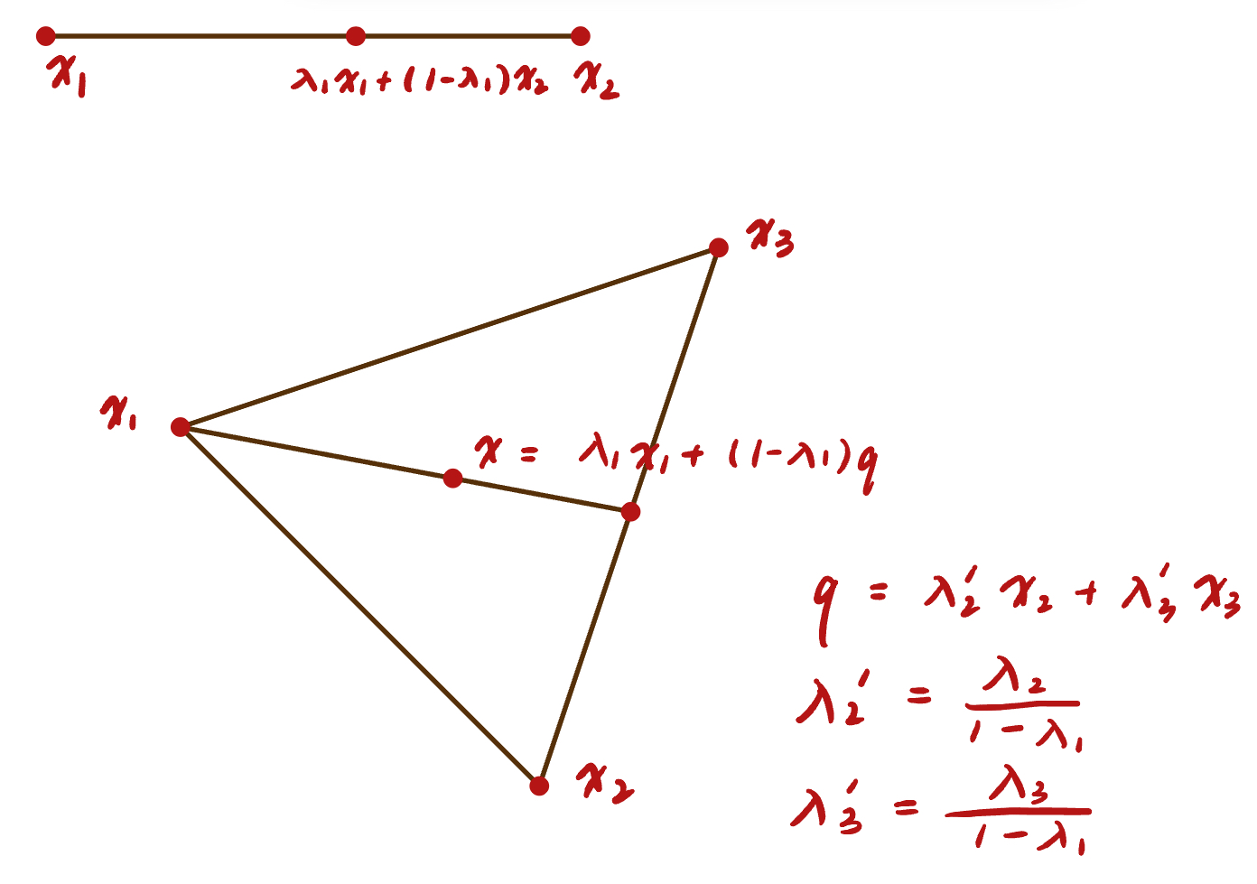
In our case, is not so we do the following. First we take the center of mass of with weights .
Then we take the center of mass of and with weights .
More explicitly, we first take . Then we take . We call this point the center of mass of with weights .
We can iterate this procedure to get the center of mass of points with nonnegative weights satisfying . This produces a singular simplex with vertices in . By Corollary 14.4.6 the diameter of this simplex is .
Remember that we want to extend of continuously. By Lemma 14.4.9 belongs to at most balls . Say these are the balls .
Let for . Then .
Using the above construction we can construct the center of mass of with weights . We set to be equal to this center of mass.
This produces a map which is maps to , is continuous and is a -GH approximation. This works if is a smooth manifold. However, in general, is only an Alexandrov space and we can not carry out this construction without more work because we have only proved Corollary 14.4.5 for smooth manifolds and not for Alexandrov spaces. However, we can carry out this procedure and construct maps as for large enough.
Likewise, we can also do the inverse which is also -Gromov-Hausdorff approximation.
Claim 14.5.1.
and are homotopy equivalences.
Proof.
Then we finished the proof.
References
- [AKP22] Stephanie Alexander, Vitali Kapovitch, and Anton Petrunin. Alexandrov geometry: foundations, 2022.
- [BBI01] D. Burago, I.U.D. Burago, and S. Ivanov. A Course in Metric Geometry. Crm Proceedings & Lecture Notes. American Mathematical Society, 2001.
- [Ber60] M. Berger. Les variétés riemanniennes -pincées. Annali della Scuola Normale Superiore di Pisa - Scienze Fisiche e Matematiche, 3e série, 14(2):161–170, 1960.
- [Ber62] M. Berger. An extension of rauch’s metric comparison theorem and some applications. Illinois Journal of Mathematics, 6(4):700 – 712, 1962.
- [Bes07] Arthur L Besse. Einstein manifolds. Springer Science & Business Media, 2007.
- [BS09] Simon Brendle and R. Schoen. Sphere theorems in geometry. Surv. Differ. Geometry, 13, 04 2009.
- [CE75] J. Cheeger and D.G. Ebin. Comparison Theorems in Riemannian Geometry. North-Holland mathematical library. North-Holland Publishing Company, 1975.
- [CG71] Jeff Cheeger and Detlef Gromoll. The splitting theorem for manifolds of nonnegative Ricci curvature. Journal of Differential Geometry, 6(1):119 – 128, 1971.
- [CG72] Jeff Cheeger and Detlef Gromoll. On the structure of complete manifolds of nonnegative curvature. Annals of Mathematics, 96(3):413–443, 1972.
- [dC92] M.P. do Carmo. Riemannian Geometry. Mathematics (Boston, Mass.). Birkhäuser, 1992.
- [Den21] Qin Deng. Hölder continuity of tangent cones and non-branching in spaces. 2021.
- [EH84] Jost Eschenburg and Ernst Heintze. An elementary proof of the cheeger-gromoll splitting theorem. Annals of Global Analysis and Geometry, 2(2):141–151, 1984.
- [EH90] J. H. Eschenburg and E. Heintze. Comparison theory for riccati equations. manuscripta mathematica, 68(1):209–214, 1990.
- [Gig22] Nicola Gigli. Introduction to the riemannian curvature dimension condition, 2022.
- [GM74] Detlef Gromoll and Wolfgang Meyer. An exotic sphere with nonnegative sectional curvature. Annals of Mathematics, 100(2):401–406, 1974.
- [GP93] Karsten Grove and Peter Petersen. A radius sphere theorem. Inventiones mathematicae, 112(1):577–583, 1993.
- [Gro82] Michael Gromov. Volume and bounded cohomology. Publications Mathématiques de l’IHÉS, 56:5–99, 1982.
- [Gro87] Grove Karsten Gromoll, Detlef. A generalization of berger’s rigidity theorem for positively curved manifolds. Annales scientifiques de l’École Normale Supérieure, 20(2):227–239, 1987.
- [Gro93] Karsten Grove. Critical point theory for distance functions, 1993.
- [GS77] Karsten Grove and Katsuhiro Shiohama. A generalized sphere theorem. Annals of Mathematics, 106(1):201–211, 1977.
- [GW09] Luis Guijarro and Gerard Walschap. Submetries vs. submersions. Revista Matematica Iberoamericana, 27:605–619, 2009.
- [Ham82] Richard S. Hamilton. Three-manifolds with positive Ricci curvature. Journal of Differential Geometry, 17(2):255 – 306, 1982.
- [Kli61] Wilhelm Klingenberg. Über riemannsche mannigfaltigkeiten mit positiver krümmung. Commentarii mathematici Helvetici, 35:47–54, 1961.
- [Lee03] J.M. Lee. Introduction to Smooth Manifolds. Graduate Texts in Mathematics. Springer, 2003.
- [Lee19] J.M. Lee. Introduction to Riemannian Manifolds. Graduate Texts in Mathematics. Springer International Publishing, 2019.
- [Lyt05] A Lytchak. Open map theorem for metric spaces. St Petersburg Mathematical Journal, 17:477–491, 01 2005.
- [Mey04] Wolfgang Meyer. Toponogov’s theorem and applications. 2004.
- [Mil56] John Milnor. On manifolds homeomorphic to the 7-sphere. Annals of Mathematics, 64(2):399–405, 1956.
- [Mye35] Sumner Byron Myers. Riemannian manifolds in the large. Duke Mathematical Journal, 1(1):39 – 49, 1935.
- [Per94a] G. Perelman. Proof of the soul conjecture of Cheeger and Gromoll. Journal of Differential Geometry, 40(1):209 – 212, 1994.
- [Per94b] G. Perelman. Proof of the soul conjecture of Cheeger and Gromoll. Journal of Differential Geometry, 40(1):209 – 212, 1994.
- [PP95] Grigori Perelman and Anton Petrunin. Quasigeodesics and gradient curves in alexandrov spaces. 1995.
- [Rau51] H. E. Rauch. A contribution to differential geometry in the large. Annals of Mathematics, 54(1):38–55, 1951.
- [Rig78] A. Rigas. Some bundles of non-negative curvature. Mathematische Annalen, 232(2):187–193, 1978.
-
[RS12]
Tapio Rajala and Karl-Theodor Sturm.
Non-branching geodesics and optimal maps in strong
c d ( k , ) -spaces. Calculus of Variations and Partial Differential Equations, 50, 07 2012. - [Sha77] V. A. Sharafutdinov. The pogorelov-klingenberg theorem for manifolds homeomorphic to rn. Siberian Mathematical Journal, 18(4):649–657, 1977.
- [Wil02] Burkhard Wilking. Manifolds with positive sectional curvature almost everywhere. Inventiones mathematicae, 148(1):117–141, 2002.
- [Wil07] Burkhard Wilking. A duality theorem for riemannian foliations in nonnegative sectional curvature. Geometric and Functional Analysis, 17(4):1297–1320, 2007.