A replica analysis of under-bagging

Abstract

Under-bagging (UB), which combines under sampling and bagging, is a popular ensemble learning method for training classifiers on an imbalanced data. Using bagging to reduce the increased variance caused by the reduction in sample size due to under sampling is a natural approach. However, it has recently been pointed out that in generalized linear models, naive bagging, which does not consider the class imbalance structure, and ridge regularization can produce the same results. Therefore, it is not obvious whether it is better to use UB, which requires an increased computational cost proportional to the number of under-sampled data sets, when training linear models. Given such a situation, in this study, we heuristically derive a sharp asymptotics of UB and use it to compare with several other standard methods for learning from imbalanced data, in the scenario where a linear classifier is trained from a two-component mixture data. The methods compared include the under-sampling (US) method, which trains a model using a single realization of the subsampled data, and the simple weighting (SW) method, which trains a model with a weighted loss on the entire data. It is shown that the performance of UB is improved by increasing the size of the majority class while keeping the size of the minority fixed, even though the class imbalance can be large, especially when the size of the minority class is small. This is in contrast to US, whose performance does not change as the size of the majority class increases, and SW, whose performance decreases as the imbalance increases. These results are different from the case of the naive bagging when training generalized linear models without considering the structure of the class imbalance, indicating the intrinsic difference between the ensembling and the direct regularization on the parameters.

1 Introduction

In the context of binary classification, class imbalance refers to the situations where one class overwhelms the other in terms of the number of data points. Learning on class imbalanced data often occurs in real-world classification tasks, such as medical data analysis (Cohen et al., 2006), image classification (Khan et al., 2018), and so on. The primary goal when training classifiers on such imbalanced data is to achieve good generalization to both minority and majority classes. However, standard supervised learning methods without any special care often results in poor generalization performance for the minority class. Therefore, special treatments are necessary and have been one of the major research topics in the machine learning (ML) community for decades.

Under-bagging (UB) (Wallace et al., 2011) is a popular and efficient method for dealing with a class imbalance that combines under-sampling (US) and bagging (Breiman, 1996). The basic idea of UB is to deal with class imbalance using under-sampling that randomly discards a portion of the majority class data to ensure an equal number of data points between the minority and the majority classes. However, this data reduction increases the variance of the estimator, because the total number of the training data is reduced. To mitigate this, UB aggregates estimators for different under-sampled data sets, similar to the aggregation performed in bootstrap aggregation (Breiman, 1996). US corresponds to a method of training a classifier on a single undersampled data. (Wallace et al., 2011) argues that UB is particularly effective for training of overparameterized models, where the number of the model parameters far exceeds the size of the training data.

There is another line of approach, that is, cost-sensitive methods, which modify the training loss at each data point depending on the class it belongs to. However, it has recently been pointed out that training overparameterized models using cost-sensitive methods requires delicate design of loss functions (Lin et al., 2017; Khan et al., 2018; Byrd & Lipton, 2019; Ye et al., 2020; Kini et al., 2021) instead of the naive weighted cross-entropy (King & Zeng, 2001) and so on. In contrast to such delicate cost-sensitive approaches, UB has the advantage of being relatively straightforward to use, since it achieves complete class balance in any under-sampled dataset.

Bagging is a natural approach to reduce the increased variance of weak learners, resulting from the smaller data size due to the resampling. However, unlike decision trees, which are the primary models used in bagging, neural networks can use simple regularization methods such as the ridge regularization to reduce the variance. In fact, it has recently been reported experimentally that naive bagging, which ignores the structure of the class balance, does not improve the classification performance of deep neural networks (Nixon et al., 2020). Furthermore, in generalized linear models (GLMs), it has been reported both theoretically (Sollich & Krogh, 1995; Krogh & Sollich, 1997; LeJeune et al., 2020; Du et al., 2023) and experimentally (Yao et al., 2021) that bagging with a specific sampling rate is exactly equivalent to the ridge regularization with a properly adjusted regularization parameter. These results indicate that naive bagging plays the role of an implicit regularization in linear models. Given these results, the question arises whether it is better to use UB, which requires an increased computational cost proportional to the number of under-sampled data sets, when training linear models or neural networks, rather than just using US and the ridge regularization.

Given the above situation, this study aims to clarify whether bagging or ridge regularization should be used when learning a linear classifier from a class-imbalanced data. Specifically, we compare the performance of classifiers obtained by UB with those obtained by (i) the under-sampling (US) method, which trains a model using a single realization of the subsampled dataset, and (ii) the simple weighting (SW) method, which trains a model with a weighted loss on the entire data, when training a linear model on two-component mixture data, through the $F$-measure. To this end, we heuristically derive a sharp characterization of the classifiers obtained by minimizing the randomly reweighted empirical risk in the asymptotic limit where the input dimension and the parameter dimension diverge at the same rate, and then use it to analyze the performance of UB, US, and SW.

The contributions of this study are summarized as follows:

• A sharp characterization of the statistical behavior of the linear classifier is derived, where the classifier is obtained by minimizing the reweighted empirical risk function on two-component mixture data, in the asymptotic limit where input dimension and data size diverge proportionally (Claim 3). This includes the properties of the estimator obtained from the under-sampled data and the simple weighted loss function. There, the statistical property of the logits for a new input is described by a small finite set of scalar quantities that is determined as a solution of nonlinear equations, which we call self-consistent equations (Definition 1). The sharp characterization of the $F$-measure is also obtained (Claim 4). The derivation is based on the replica method of statistical physics (Mézard et al., 1987; Charbonneau et al., 2023; Montanari & Sen, 2024).

• Using the derived sharp asymptotics, it is shown that the estimators obtained by UB have higher generalization performance in terms of $F$-measure than those obtained by US or SW. Although the performance of UB in terms of the $F$-measure is improved by increasing the size of the majority class while keeping the size of the minority class fixed, the performance of US does not depend on the size of the excess examples of the majority class (Section 4.1). This result is clearly different from the case of the naive bagging in training GLMs without considering the structure of the class imbalance, where the ensembling and ridge regularization yield the same performance. That is, the ensembling and the regularization are different when the data structure is taken into account. The performance of SW is even worse, i.e., its performance on the $F$-measure decreases as the size of the majority class increases, leading to a catastrophic performance degradation when training from data with a small minority class (Section 4.2).

• Furthermore, it is shown that UB is robust to the existence of the interpolation phase transition, where data goes from linearly separable to inseparable training data (Section 4.1.1). In contrast, the performance of the interpolator obtained from a single realization of balanced data is affected by such a phase transition as reported in the previous study (Mignacco et al., 2020).

1.1 Further related works

Learning under class imbalance is a classic and notorious problem in data mining and ML. In fact, the development of dealing with imbalanced data was selected as “10 CHALLENGING PROBLEMS IN DATA MINING RESEARCH” (Yang & Wu, 2006) about 20 years ago in the data mining community. Due to its practical relevance, a lot of methodological research has been continuously conducted and are summarized in reviews (He & Garcia, 2009; Longadge & Dongre, 2013; Johnson & Khoshgoftaar, 2019; Mohammed et al., 2020).

Learning methods for imbalanced data can broadly be classified into two categories: cost- and data-level ones. In cost-sensitive methods, the cost function itself is modified to assign different costs to each class. A classic method includes a weighting method that assigns a different constant multiplier to the loss at each data point depending on the class it belongs to. However, when training overparameterized models, it has been pointed out that a classic weighting method fails and a more delicate design of the loss function is required to properly adjust the margins between classes (Lin et al., 2017; Khan et al., 2018; Byrd & Lipton, 2019; Ye et al., 2020; Kini et al., 2021). In data-level methods, the training data itself is modified to create a class-balanced dataset using resampling methods. The major approaches include US (Drummond et al., 2003), which randomly discards some of the majority class data, and SMOTE (Chawla et al., 2002), which creates synthetic minority data points. Although the literature (Wallace et al., 2011) argues that a combination of US and bagging is effective for learning overparameterized models, the comparison with other regularization techniques is not discussed.

Technically, our work is an analysis of the sharp asymptotics of resampling methods in which the input dimension and the size of the data set diverge at the same rate. The analysis of such sharp asymptotics of ML methods in this asymptotic regime has been actively carried out since the 1990s, using techniques from statistical physics (Opper & Kinzel, 1996; Opper, 2001; Engel & Van den Broeck, 2001). Recently, it has become one of the standard analytical approaches, and various mathematical techniques have also been developed to deal with it. The salient feature of this proportional asymptotic regime is that the macroscopic properties of the learning results, such as the predictive distribution and the generalization error, do not depend on the details of the realization of the training data, when using convex loss. That is, the fluctuations of these quantities with respect to the training data vanish, allowing us to make sharp theoretical predictions (Barbier et al., 2019; Charbonneau et al., 2023). The technical tools for analyzing such asymptotics include the replica method (Gerace et al., 2020; Charbonneau et al., 2023; Montanari & Sen, 2024), convex Gaussian minimax theorem (Thrampoulidis et al., 2018), random matrix theory (Mei & Montanari, 2022), adaptive interpolation method (Barbier & Macris, 2019; Barbier et al., 2019), approximate message passing (Sur & Candès, 2019; Feng et al., 2022), and so on.

Resampling methods have also been studied in the same proportional asymptotics. (Sollich & Krogh, 1995; Krogh & Sollich, 1997; Malzahn & Opper, 2001; 2002; 2003; LeJeune et al., 2020; Ando & Komaki, 2023; Bellec & Koriyama, 2024; Clarté et al., 2024; Patil & LeJeune, 2023) analyze the performance of the ensemble average of the linear models, and (Takahashi, 2023) analyzes the distribution of the ensemble average of the de-biased elastic-net estimator (Javanmard & Montanari, 2014a; b). However, these analyses do not address the structure of the class imbalance. Ensembling in random feature models as a method to reduce the effect of random initialization are also considered in (D’Ascoli et al., 2020; Loureiro et al., 2022). Furthermore, the literature (Obuchi & Kabashima, 2019; Takahashi & Kabashima, 2019; 2020) derives the properties of the estimators trained on the resampled data set in the analysis of the dynamics of approximate message passing algorithms that yield exact results in Gaussian or rotation-invariant feature data.

Notation	Description
$N$	input dimension
$M^{+}$	size of the positive examples (assumed to be the minority class)
$M^{-}$	size of the negative examples (assumed to be the majority class)
$M$	$M^{+}+M^{-}$, the size of the overall training data
$\mu,\nu$	indices of data points
$i,j$	indices of the weight vector $\mathbf{\boldsymbol{w}}$
$[n]$	for an positive integer $n$, the set $\{1,\dots,n\}$
$v_{i}$	$i$-th element of a vector $\mathbf{\boldsymbol{v}}$
$\mathbf{\boldsymbol{x}}\cdot\mathbf{\boldsymbol{y}}$	for vectors $\mathbf{\boldsymbol{x}},\mathbf{\boldsymbol{y}}\in\mathbb{R}^{N}$, the inner product of them: $\mathbf{\boldsymbol{x}}\cdot\mathbf{\boldsymbol{v}}=\sum_{i=1}^{N}x_{i}y_{i}$.
$\mathbf{\boldsymbol{1}}_{N}$	an $N$-dimensional vector $(1,1,\dots,1)\in\mathbb{R}^{N}$
$\mbox{\rm 1}\mbox{\rm l}(\cdot)$	indicator function
${\mathcal{N}}(\mu,\sigma^{2})$	Gaussian density with mean $\mu$ and variance $\sigma^{2}$
${\rm Poisson}(\mu_{\ast})$	Poisson distribution with mean $\mu_{\ast}$
iid	independent and identically distributed
$\mathbb{E}_{X\sim p_{X}}[f(X)]$	Expectation regarding random variable $X$
	where $p$ is the density function for the random variable $X$
	(lower subscript $X\sim p_{X}$ or $p_{X}$ can be omitted if there is no risk of confusion)
${\mathbb{V}}_{X\sim p_{X}}[f(X)]$	Variance: $\mathbb{E}[f(X)^{2}]-\mathbb{E}[f(X)]^{2}$
	(lower subscript $X\sim p_{X}$ or $p_{X}$ can be omitted if there is no risk of confusion)
$\delta_{\rm d}(\cdot)$	Dirac’s delta function

Table 1: Notations

1.2 Notations

Throughout the paper, we use some shorthand notations for convenience. We summarize them in Table 1.

2 Problem setup

This section presents the problem formulation and our interest in this work. First, the assumptions about the data generation process are described, and then the estimator of the interest is introduced.

Let $D^{+}=\{(\mathbf{\boldsymbol{x}}_{\mu}^{+},1)\}_{\mu=1}^{M^{+}},\mathbf{\boldsymbol{x}}_{\mu}^{+}\in\mathbb{R}^{N}$ and $D^{-}=\{(\mathbf{\boldsymbol{x}}_{\nu}^{-},-1)\}_{\nu=1}^{M^{-}},\mathbf{\boldsymbol{x}}_{\nu}^{-}\in\mathbb{R}^{N}$ be the sets of positive and negative examples; in total we have $M=M^{+}+M^{-}$ examples. In this study, the positive class is assumed to be the minority class, that is, $M^{+}<M^{-}$. Also, it is assumed that positive and negative samples are drawn from a mixture model whose centroids are located at $\pm\mathbf{\boldsymbol{v}}/\sqrt{N}$ with $\mathbf{\boldsymbol{v}}\in\mathbb{R}^{N}$ being a fixed vector as follows:

$$\mathbf{\boldsymbol{x}}_{\mu}^{+} =\frac{1}{\sqrt{N}}\mathbf{\boldsymbol{v}}+\mathbf{\boldsymbol{z}}_{\mu}^{+},$$ (1)

$$\mathbf{\boldsymbol{x}}_{\nu}^{-} =-\frac{1}{\sqrt{N}}\mathbf{\boldsymbol{v}}+\mathbf{\boldsymbol{z}}_{\nu}^{-},$$ (2)

where $\mathbf{\boldsymbol{z}}_{\mu}^{+}$ and $\mathbf{\boldsymbol{z}}_{\nu}^{-}$ are noise vectors. We assume that $z_{\mu,i}^{+},z_{\nu,i}^{-}\sim_{\rm iid}p_{z},\mu\in[M^{+}],\nu\in[M^{-}],i\in[N]$, where the mean and the variance of $p_{z}$ are zero and $\Delta$, respectively, and also the higher order moments are finite. From the rotational symmetry, we can fix the direction of the vector $\mathbf{\boldsymbol{v}}$ as $\mathbf{\boldsymbol{v}}=(1,1,\dots,1)^{\top}$ without loss of generality. The goal is to obtain a classifier that generalize well to both positive and negative inputs from $D=D^{+}\cup D^{-}$. We focus on the training of the linear model, i.e., the model’s output $f(\mathbf{\boldsymbol{x}})$ at an input $\mathbf{\boldsymbol{x}}$ is a function of a linear combination of the weight $\mathbf{\boldsymbol{w}}$ and the bias $B$:

$$f_{\rm model}(\mathbf{\boldsymbol{x}})=f\left(\frac{1}{\sqrt{N}}\mathbf{\boldsymbol{x}}\cdot\mathbf{\boldsymbol{w}}+B\right),$$ (3)

where the factor $1/\sqrt{N}$ is introduced to ensure that the logit $\mathbf{\boldsymbol{x}}\cdot\mathbf{\boldsymbol{w}}/\sqrt{N}+B$ should be of ${\mathcal{O}}(1)$, and $f$ is a some nonlinear function. In the following, we denote $\mathbf{\boldsymbol{\theta}}$ for the shorthand notation of the linear model’s parameter.

To obtain a classifier, we consider minimizing the following randomly reweighted empirical risk function:

$$\hat{\mathbf{\boldsymbol{\theta}}}(\{c_{\mu}^{+}\},\{c_{\nu}^{-}\},D)=\operatorname*{arg\,min}_{(\mathbf{\boldsymbol{w}},b)\in\mathbb{R}^{N+1}} \sum_{\mu=1}^{M^{+}}c_{\mu}^{+}l^{+}(\mathbf{\boldsymbol{x}}_{\mu}^{+}\cdot\mathbf{\boldsymbol{w}}/\sqrt{N}+b)$$

$$+\sum_{\nu=1}^{M^{-}}c_{\nu}^{-}l^{-}(\mathbf{\boldsymbol{x}}_{\nu}^{-}\cdot\mathbf{\boldsymbol{w}}/\sqrt{N}+b)+\lambda\sum_{i=1}^{N}r(w_{i}),$$ (4)

when the bias $B$ is estimated by minimizing the cost function, and

$$\hat{\mathbf{\boldsymbol{w}}}(\{c_{\mu}^{+}\},\{c_{\nu}^{-}\},D)=\operatorname*{arg\,min}_{\mathbf{\boldsymbol{w}}\in\mathbb{R}^{N}} \sum_{\mu=1}^{M^{+}}c_{\mu}^{+}l^{+}(\mathbf{\boldsymbol{x}}_{\mu}^{+}\cdot\mathbf{\boldsymbol{w}}/\sqrt{N}+\bar{B})$$

$$+\sum_{\nu=1}^{M^{-}}c_{\nu}^{-}l^{-}(\mathbf{\boldsymbol{x}}_{\nu}^{-}\cdot\mathbf{\boldsymbol{w}}/\sqrt{N}+\bar{B})+\lambda\sum_{i=1}^{N}r(w_{i}),$$ (5)

when the bias is fixed as $\bar{B}$ during the training. Here, $l^{+}$ and $l^{-}$ are the convex loss for positive and negative examples, respectively. For example, the choice of $l^{+}(x)=-\log(\sigma(x))$ and $l^{-}(x)=-\log(1-\sigma(x))$, with $\sigma(\cdot)$ being the sigmoid function, yields the cross-entropy loss. Also, $c_{\mu}^{+}\sim_{\rm iid}p_{c}^{+}$ and $c_{\nu}^{-}\sim_{\rm iid}p_{c}^{-}$ are the random coefficients that represent the effect of the resampling or the weighting. In the following, we use the notation $\mathbf{\boldsymbol{c}}\equiv\{c_{\mu}^{+}\}_{\mu=1}^{M^{+}}\cup\{c_{\nu}^{-}\}_{\nu=1}^{M^{-}}\sim p_{c}$. Finally, $\lambda r(x)=\lambda x^{2}/2$ is the ridge regularization for the weight vector with a regularization parameter $\lambda\in(0,\infty)$.

By appropriately specifying the distribution $p_{c}^{\pm}$, the estimators (4) and (5) can represent estimators for different types of costs for resampled or reweighted data as follows:

• US without replacement (subsampling):

  $$p_{c}^{+}(c^{+}) =\delta_{\rm d}(c^{+}-1)$$ (6)

  $$p_{c}^{+}(c^{-}) =\mu_{\ast}\delta_{\rm d}(c^{-}-1)+(1-\mu_{\ast})\delta_{\rm d}(c^{-}),$$ (7)

  where $\mu_{\ast}\in(0,1]$ be the resampling rate. $\mu_{\ast}=M^{+}/M^{-}$ is the natural choice to balance the size of the sizes of positive and negative examples.

• US with replacement (bootstrap):

  $$p_{c}^{+}(c^{+}) =\delta_{\rm d}(c^{+}-1),$$ (8)

  $$p_{c}^{-} ={\rm Poisson}(\mu_{\ast}),$$ (9)

  where $\mu_{\ast}\in(0,1]$ be the resampling rate.

• Simple weighting:

  $$p_{c}^{+}(c^{+}) =\delta_{\rm d}(c^{+}-\gamma^{+}),$$ (10)

  $$p_{c}^{-}(c^{-}) =\delta_{\rm d}(c^{-}-\gamma^{-}),$$ (11)

  where $\gamma^{+},\gamma^{-}\in(0,\infty)$ is the reweighting coefficient for the positive and negative classes. $\gamma^{+}=(M^{+}+M^{-})/(2M^{+}),\gamma^{-}=(M^{+}+M^{-})/(2M^{-})$ is the standard choice used in major ML packages such as the scikit-learn (Pedregosa et al., 2011; King & Zeng, 2001).

The ensemble average of the prediction for a new input $\mathbf{\boldsymbol{x}}$ is thus obtained as follows:

$$\begin{cases}\mathbb{E}_{\mathbf{\boldsymbol{\mathbf{\boldsymbol{c}}}}}\left[\mathbf{\boldsymbol{x}}\cdot\hat{\mathbf{\boldsymbol{w}}}(\mathbf{\boldsymbol{c}},D)/\sqrt{N}+\hat{B}(\mathbf{\boldsymbol{c}},D)\right],&{\rm when~{}bias~{}is~{}estimated\vspace{2truemm}}\\ \mathbb{E}_{\mathbf{\boldsymbol{\mathbf{\boldsymbol{c}}}}}\left[\mathbf{\boldsymbol{x}}\cdot\hat{\mathbf{\boldsymbol{w}}}(\mathbf{\boldsymbol{c}},D)/\sqrt{N}+\bar{B}\right],&{\rm when~{}bias~{}is~{}fixed}\end{cases}$$ (12)

In this study, we focus on the case of subsampling as a method of resampling (6)-(7), since the the computational cost is usually smaller than the bootstrap.

The purpose of this study is twofold: the first is to characterize how the prediction $\mathbf{\boldsymbol{x}}\cdot\hat{\mathbf{\boldsymbol{w}}}(\mathbf{\boldsymbol{c}},D)/\sqrt{N}+\hat{B}(\mathbf{\boldsymbol{c}},D)~{}({\rm or~{}}\bar{B})$ depends statistically on $\mathbf{\boldsymbol{x}}$ and $\mathbf{\boldsymbol{c}}$, and the other is to clarify the difference in performance with the UB obtained by (12) and the US or SW obtained by (4) or (5) with fixed $\mathbf{\boldsymbol{c}}$. We are interested in the generalization performance for both positive and negative inputs. Therefore, we will evaluate the generalization performance using the $F$-measure, the weighted harmonic mean of specificity and recall.

To characterize the properties of the estimators (4) and (5), we consider the large system limit where $N,M^{+},M^{-}\to\infty$, keeping their ratios as $(M^{+}/N,M^{-}/N)=(\alpha^{+},\alpha^{-})\in(0,\infty)^{2}$. In this asymptotic limit, the behavior of the estimators (4) and (5) can be sharply characterized as shown in the next section. We call this asymptotic limit as large system limit (LSL). In the following, $N\to\infty$ represents the LSL as a shorthand notation to avoid cumbersome notation.

3 Asymptotics of the estimator for the randomized cost function

In this section, we present the asymptotic properties of the estimators (4) and (5) for the randomized cost functions. It is described by a small finite set of scalar quantities determined as a solution of nonlinear equations, which we refer to as self-consistent equations. The derivation is outlined in Appendix A.

As noted in the related works section, the salient feature of the asymptotics in the LSL is that the macroscopic properties of the learning results, such as the predictive distribution, typically do not depend on each realization of the training data. In this paper, we assume these concentration properties in advance to derive the formulas for the asymptotic properties.

Assumption 1 (Concentration of the macroscopic properties of the learning results)

We assume that the macroscopic properties of the estimators (4)-(5) will concentrate at LSL. Concretely, we assume that the values of $(N^{-1}\sum_{i}\mathbb{E}_{\mathbf{\boldsymbol{c}}}[\hat{w}_{i}(\mathbf{\boldsymbol{c}},D)]^{2},N^{-1}\sum_{i}\mathbb{E}_{\mathbf{\boldsymbol{c}}}[\hat{w}_{i}(\mathbf{\boldsymbol{c}},D)],N^{-1}\sum_{i}{\mathbb{V}}_{\mathbf{\boldsymbol{c}}}[\hat{w}_{i}(\mathbf{\boldsymbol{c}},D)],\hat{B}(\mathbf{\boldsymbol{c}},D))$ does not fluctuate with respect to the realization of $D$ at LSL. Also, Let $\mathbf{\boldsymbol{x}}^{\pm}=\pm\mathbf{\boldsymbol{v}}/\sqrt{N}+\mathbf{\boldsymbol{z}},~{}z_{i}\sim_{\rm iid}p_{z},i\in[N]$ be a new input. We assume that the distribution of the prediction for this new input $\hat{s}^{\pm}(\mathbf{\boldsymbol{c}},D)=\mathbf{\boldsymbol{x}}^{\pm}\cdot\hat{\mathbf{\boldsymbol{w}}}(\mathbf{\boldsymbol{c}},D)/\sqrt{N}+\hat{B}(\mathbf{\boldsymbol{c}},D)$ (or $\bar{B}$ when the bias is fixed) with respect to $\mathbf{\boldsymbol{c}}$ and $\mathbf{\boldsymbol{z}}$ does not fluctuate with respect to the realization of $D$ at LSL.

Under the above assumption, we obtain the following prediction of the behavior of the estimators (4)-(5).

First, let us define the self-consistent equations that determines a set of scalar quantities $B\in\mathbb{R},\Theta=(q,m,\chi,v)\in(0,\infty)\times\mathbb{R}\times(0,\infty)\times(0,\infty)$ and $\hat{\Theta}=(\hat{Q},\hat{m},\hat{\chi},\hat{v})\in(0,\infty)\times\mathbb{R}\times(0,\infty)\times(0,\infty)$ that characterize the statistical behavior of (4) and (5). The readers interested in the implications of these quantities can skip Definition 1 and Claim 1, and proceed to Claim 2.

Definition 1 (Self-consistent equations)

The set of quantities $\Theta$ and $\hat{\Theta}$ are defined as the solution of the following set of non-linear equations that are referred to as self-consistent equations. Let $\hat{\mathsf{w}}$ and $\hat{\mathsf{u}}^{\pm}$ be the solution of the following one-dimensional randomized optimization problems:

$$\hat{\mathsf{w}} =\operatorname*{arg\,min}_{w\in\mathbb{R}}\frac{\hat{Q}}{2}w^{2}-h_{w}w+\lambda r(w),$$ (13)

$$\hat{\mathsf{u}}^{\pm} =\operatorname*{arg\,min}_{u\in\mathbb{R}}\frac{u^{2}}{2\chi\Delta}+c^{\pm}l^{\pm}(u+h_{u}^{\pm}),$$ (14)

where

$$h_{w} =\hat{m}+\sqrt{\hat{\chi}}\xi_{w}+\sqrt{\hat{v}}\eta_{w},\quad\xi_{w},\eta_{w}\sim{\mathcal{N}}(0,1),$$ (15)

$$h_{u}^{\pm} =B\pm m+\sqrt{q}\xi_{u}+\sqrt{v}\eta_{u},\quad\xi_{u},\eta_{u}\sim{\mathcal{N}}(0,\Delta),$$ (16)

and $c^{+}\sim p_{c}^{+},c^{-}\sim p_{c}^{-}$. Then, the self-consistent equations are given as follows:

$$\chi =E_{\xi_{w},\eta_{w}\sim{\mathcal{N}}(0,1)}\left[\frac{d}{dh_{w}}\hat{\mathsf{w}}\right],$$ (17)

$$q =\mathbb{E}_{\xi_{w}\sim{\mathcal{N}}(0,1)}\left[\mathbb{E}_{\eta_{w}\sim{\mathcal{N}}(0,1)}[\hat{\mathsf{w}}]^{2}\right],$$ (18)

$$m =E_{\xi_{w},\eta_{w}\sim{\mathcal{N}}(0,1)}\left[\hat{\mathsf{w}}\right],$$ (19)

$$v =\mathbb{E}_{\xi_{w}\sim{\mathcal{N}}(0,1)}\left[{\mathbb{V}}_{\eta_{w}\sim{\mathcal{N}}(0,1)}[\hat{\mathsf{w}}]\right],$$ (20)

$$\hat{Q} =-\frac{1}{\chi}\mathbb{E}_{\xi_{u},\eta_{u}\sim{\mathcal{N}}(0,\Delta),c^{\pm}\sim p_{c}^{\pm}}\left[\alpha^{+}\frac{d}{dh_{u}^{+}}\hat{\mathsf{u}}^{+}+\alpha^{-}\frac{d}{dh_{u}^{-}}\hat{\mathsf{u}}^{-}\right],$$ (21)

$$\hat{\chi} =\frac{1}{\Delta\chi^{2}}\mathbb{E}_{\xi_{u}\sim{\mathcal{N}}(0,\Delta)}\left[\alpha^{+}\mathbb{E}_{\eta_{u}\sim{\mathcal{N}}(0,\Delta),c^{+}\sim p_{c}^{+}}[\hat{\mathsf{u}}^{+}]^{2}+\alpha^{-}\mathbb{E}_{\eta_{u}\sim{\mathcal{N}}(0,\Delta),c^{-}\sim p_{c}^{-}}[\hat{\mathsf{u}}^{-}]^{2}\right],$$ (22)

$$\hat{m} =\frac{1}{\Delta\chi}\mathbb{E}_{\xi_{u},\eta_{u}\sim{\mathcal{N}}(0,\Delta),c^{\pm}\sim p_{c}^{\pm}}\left[\alpha^{+}\hat{\mathsf{u}}^{+}-\alpha^{-}\hat{\mathsf{u}}^{-}\right],$$ (23)

$$\hat{v} =\frac{1}{\Delta\chi^{2}}\mathbb{E}_{\xi_{u}\sim{\mathcal{N}}(0,\Delta)}\left[\alpha^{+}{\mathbb{V}}_{\eta_{u}\sim{\mathcal{N}}(0,\Delta),c^{+}\sim p_{c}^{+}}[\hat{\mathsf{u}}^{+}]+\alpha^{-}{\mathbb{V}}_{\eta_{u}\sim{\mathcal{N}}(0,\Delta),c^{-}\sim p_{c}^{-}}[\hat{\mathsf{u}}^{-}]\right].$$ (24)

Furthermore, depending on whether the bias is estimated or fixed, the following equation is added to the self-consistent equation

$$\begin{cases}0=\mathbb{E}_{\xi_{u},\eta_{u}\sim{\mathcal{N}}(0,\Delta),c^{\pm}\sim p_{c}^{\pm}}\left[\alpha^{+}\hat{\mathsf{u}}^{+}+\alpha^{-}\hat{\mathsf{u}}^{-}\right],&{\rm when~{}bias~{}is~{}estimated\vspace{2truemm}}\\ B=\bar{B},&{\rm when~{}bias~{}is~{}fixed}\end{cases}.$$ (25)

It is also noteworthy to comment on the interpretation of the parameter $B$ and $(q,m,v)$ in the self-consistent equations.

Claim 1 (Interpretation of the parameters $\Theta$)

At the LSL, the solution of the self-consistent equations are related with the weight vector $\hat{\mathbf{\boldsymbol{w}}}(\mathbf{\boldsymbol{c}},D)$ as follows:

$$q =\lim_{N\to\infty}\frac{1}{N}\sum_{i=1}^{N}\mathbb{E}_{\mathbf{\boldsymbol{c}}}\left[\hat{w}_{i}(\mathbf{\boldsymbol{c}},D)\right]^{2},$$ (26)

$$m =\lim_{N\to\infty}\frac{1}{N}\sum_{i=1}^{N}\mathbb{E}_{\mathbf{\boldsymbol{c}}}\left[\hat{w}_{i}(\mathbf{\boldsymbol{c}},D)\right],$$ (27)

$$v =\lim_{N\to\infty}\frac{1}{N}\sum_{i=1}^{N}{\mathbb{V}}_{\mathbf{\boldsymbol{c}}}\left[\hat{w}_{i}(\mathbf{\boldsymbol{c}},D)\right],$$ (28)

$$B =\begin{cases}\lim_{N\to\infty}\hat{B}(\mathbf{\boldsymbol{c}},D),&{\rm when~{}bias~{}is~{}estiamted\vspace{2truemm}}\\ \bar{B},&{\rm when~{}bias~{}is~{}fixed}\end{cases}$$ (29)

That is, $q,m,v,B$ represents the squared norm of the averaged weight vector, the inner product with the cluster center, the variance with respect to the resampling, and the bias, respectively, at LSL.

Using the solution of the self-consistent equations, we can obtain the following expression for the average of the prediction.

Claim 2 ($l$-th moments of the predictor)

Let $(B,m,q,v)$ be the solution of the self-consistent equation in Definition 1, and let $l=1,2,\dots\in{\mathbb{N}}$ be the non-negative integer. Also, $\hat{s}^{\pm}(\mathbf{\boldsymbol{c}},D)\equiv\mathbf{\boldsymbol{x}}^{\pm}\cdot\hat{\mathbf{\boldsymbol{w}}}(\mathbf{\boldsymbol{c}},D)/\sqrt{N}+\hat{B}(\mathbf{\boldsymbol{c}},D)$ and $\hat{s}^{\pm}(\mathbf{\boldsymbol{c}},D)\equiv\mathbf{\boldsymbol{x}}^{\pm}\cdot\hat{\mathbf{\boldsymbol{w}}}(\mathbf{\boldsymbol{c}},D)/\sqrt{N}+\bar{B}$ be the predictions of the estimators (4) and (5) for an input $\mathbf{\boldsymbol{x}}^{\pm}$ which is generated as

$$\mathbf{\boldsymbol{x}}^{\pm}=\pm\mathbf{\boldsymbol{1}}_{N}/\sqrt{N}+\mathbf{\boldsymbol{z}},\quad z_{i}\sim_{\rm iid}p_{z},i\in[N].$$ (30)

Then, for any $l$, we can obtain the following result regardless of whether the bias is estimated or not:

$$\mathbb{E}_{D,\mathbf{\boldsymbol{x}}^{\pm}}\left[\mathbb{E}_{\mathbf{\boldsymbol{c}}}[\psi(\hat{s}^{\pm})]^{l}\right]=\mathbb{E}_{\xi_{u}\sim{\mathcal{N}}(0,\Delta)}\left[\mathbb{E}_{\eta_{u}\sim{\mathcal{N}}(0,\Delta)}[\psi(B\pm m+\sqrt{q}\xi_{u}+\sqrt{v}\eta_{u})]^{l}\right],$$ (31)

where $\psi$ is arbitrary as long as the above integrals are convergent.

This result indicates that the fluctuation with respect to resampling conditioned by $\mathbf{\boldsymbol{x}}$ is effectively described by the Gaussian random variable $\eta_{u}$, and the fluctuation with respect to the noise term in $\mathbf{\boldsymbol{x}}$ is described by the Gaussian random variable $\xi_{u}$. Schematically, this behavior can be represented as follows:

$$\hat{s}^{\pm}=\underset{\rm bias}{\uwave{B}}+\underset{\begin{subarray}{c}\rm correlation~{}with\\ \rm the~{}cluster~{}center\end{subarray}}{\uwave{(\pm m)}}+\underset{\begin{subarray}{c}{\rm fluctuation~{}from}\\ {\rm the~{}noise~{}}\mathbf{\boldsymbol{z}}\end{subarray}}{\uwave{\sqrt{q}\xi_{u}}}+\underset{\begin{subarray}{c}{\rm fluctuation~{}from}\\ {\rm random~{}reweighting~{}}\mathbf{\boldsymbol{c}}\\ {\rm conditioned~{}by~{}}\mathbf{\boldsymbol{x}}\end{subarray}}{\uwave{\sqrt{v}\eta_{u}}}.$$ (32)

Therefore, the distribution of the prediction averaged over $K$-realization of the reweighing coefficient $\{\mathbf{\boldsymbol{c}}_{k}\}_{k=1}^{K}$ can be described as follows.

Claim 3 (Distribution of the averaged prediction)

Let $(B,m,q,v)$ be the solution of the self-consistent equation in Definition 1. Then, the distribution of $\hat{s}_{K}^{\pm}=\frac{1}{K}\sum_{k=1}^{K}\mathbf{\boldsymbol{x}}\cdot\hat{\mathbf{\boldsymbol{w}}}(\mathbf{\boldsymbol{c}}_{k},D)/\sqrt{N}+\hat{B}(\mathbf{\boldsymbol{c}}_{k},D)$ (or $\bar{B}$ when the bias is fixed), the prediction averaged over $K$-realization of the reweighing coefficient $\{\mathbf{\boldsymbol{c}}_{k}\}_{k=1}^{K}$ when the noise term $\mathbf{\boldsymbol{z}}$ fluctuates, is equal to that of the following random quantity:

$$\hat{s}^{\pm}_{K}=B\pm m+\sqrt{q}\xi_{u}+\sqrt{\frac{v}{K}}\eta_{u},\quad\xi_{u},\eta_{u}\sim{\mathcal{N}}(0,\Delta).$$ (33)

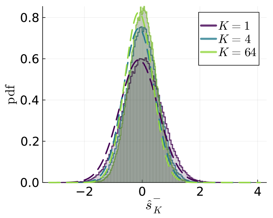
(a) $(\frac{M^{+}}{M},y,N)=(0.01,-1,2^{10})$

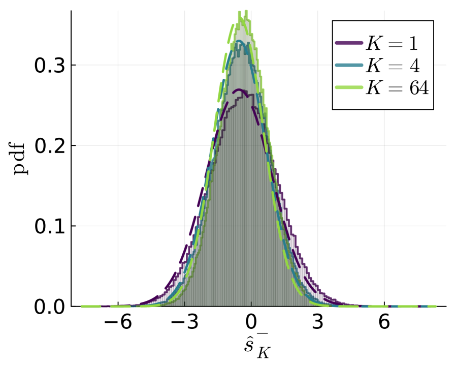
(b) $(\frac{M^{+}}{M},y,N)=(0.05,-1,2^{10})$

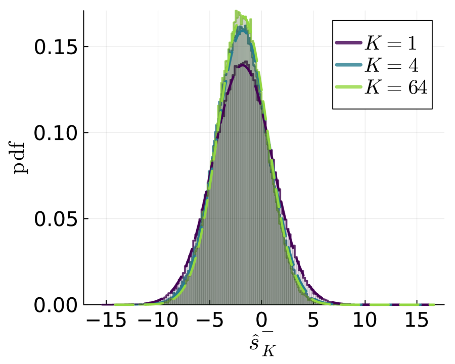
(c) $(\frac{M^{+}}{M},y,N)=(0.2,-1,2^{10})$

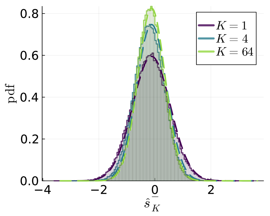
(d) $(\frac{M^{+}}{M},y,N)=(0.01,-1,2^{13})$

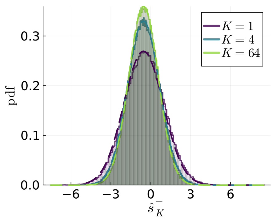
(e) $(\frac{M^{+}}{M},y,N)=(0.05,-1,2^{13})$

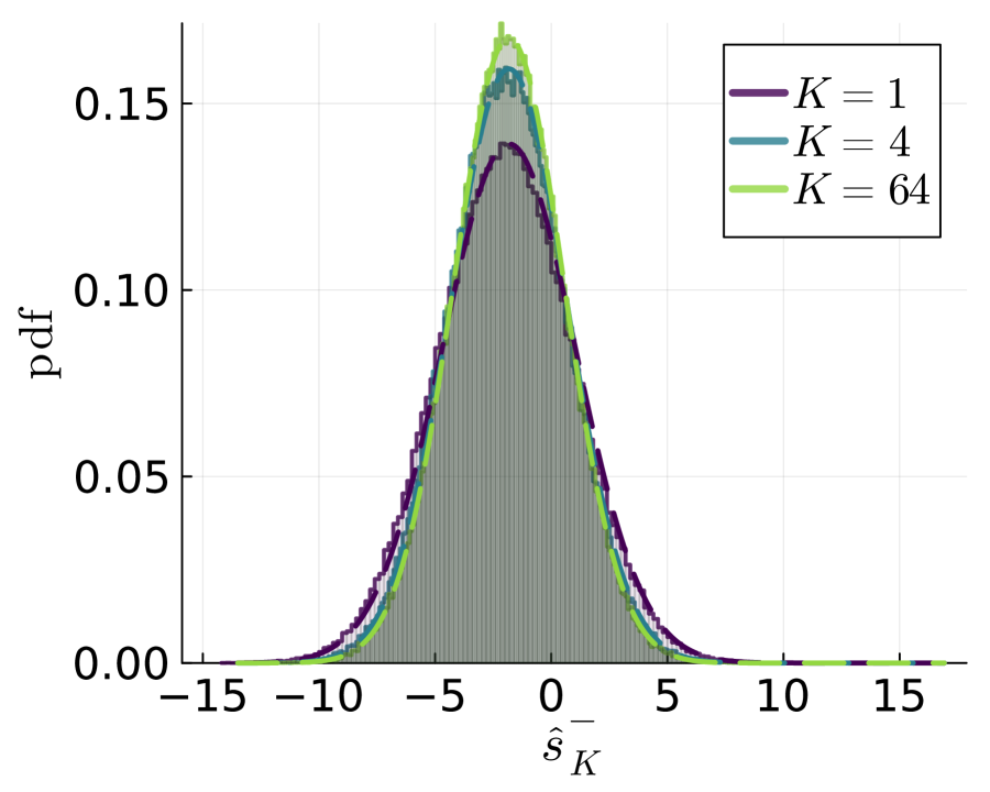
(f) $(\frac{M^{+}}{M},y,N)=(0.2,-1,2^{13})$

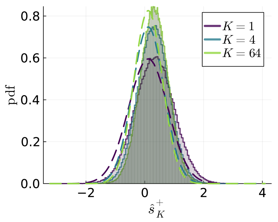
(g) $(\frac{M^{+}}{M},y,N)=(0.01,+1,2^{10})$

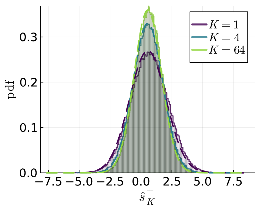
(h) $(\frac{M^{+}}{M},y,N)=(0.05,+1,2^{10})$

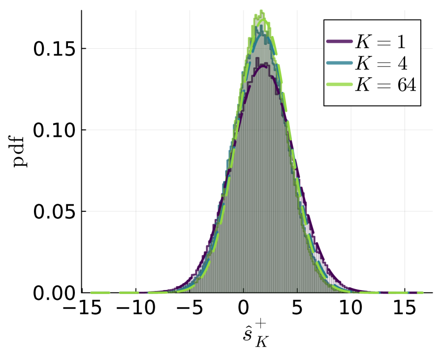
(i) $(\frac{M^{+}}{M},y,N)=(0.2,+1,2^{10})$

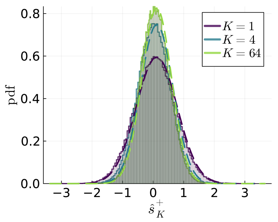
(j) $(\frac{M^{+}}{M},y,N)=(0.01,+1,2^{13})$

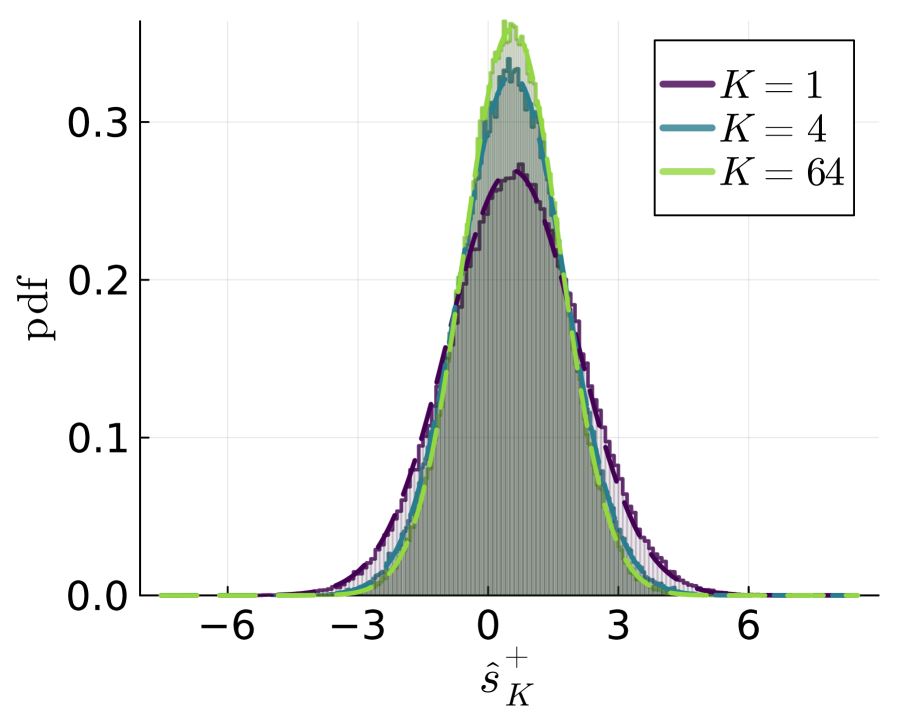
(k) $(\frac{M^{+}}{M},y,N)=(0.05,+1,2^{13})$

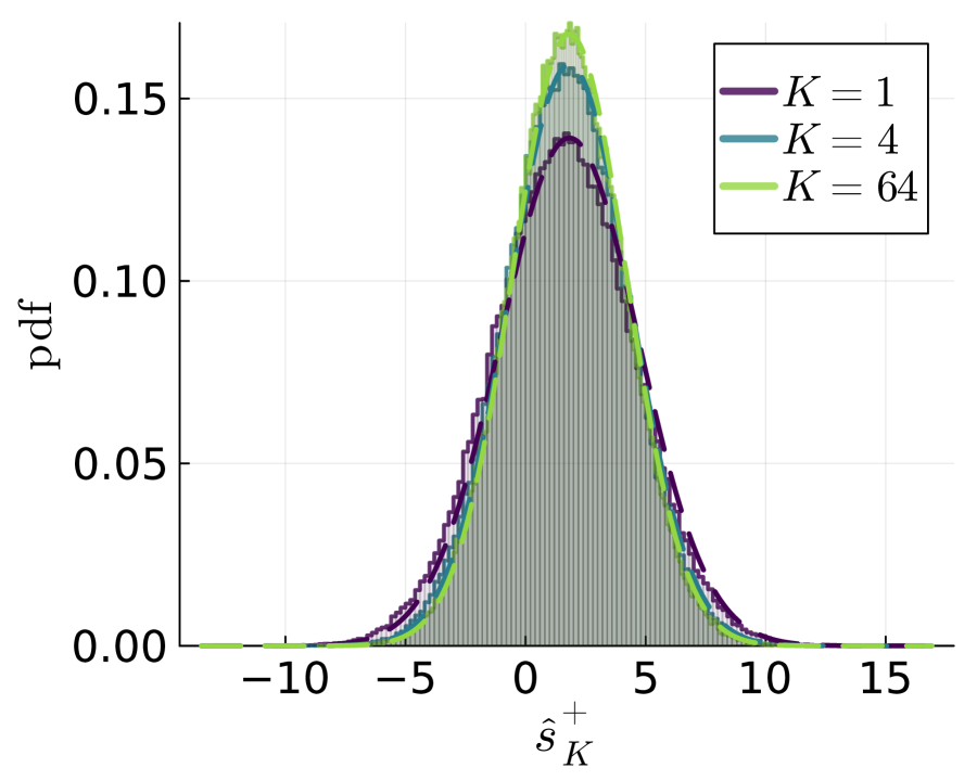
(l) $(\frac{M^{+}}{M},y,N)=(0.2,+1,2^{13})$

Figure 1: Comparison between the empirical distribution of $\hat{s}_{K}^{\pm}$ (histogram), which is obtained by a single realization of the training data $D$ of finite size, and the theoretical prediction in Claim 3 (dashed). Different colors represent resampling averages with different numbers of realizations of reweighting coefficient $\mathbf{\boldsymbol{c}}$.

The US, which uses a single realization of the resampled data set, corresponds to the case of $K=1$.

Using the above result, one obtains the expression of the $F$-measure as follows:

Claim 4 ($F$-measure)

Let $(q,m,v,B)$ be the solution of the self-consistent equations in Definition 1. Then, for $\hat{s}_{K}^{\pm}=\frac{1}{K}\sum_{k=1}^{K}\mathbf{\boldsymbol{x}}\cdot\hat{\mathbf{\boldsymbol{w}}}(\mathbf{\boldsymbol{c}}_{k},D)/\sqrt{N}+\hat{B}(\mathbf{\boldsymbol{c}}_{k},D)$ (or $\bar{B}$ when the bias is fixed), the prediction averaged over $K$-realization of the reweighing coefficient $\{\mathbf{\boldsymbol{c}}_{k}\}_{k=1}^{K}$, the specificity ${\mathcal{S}}$, the recall ${\mathcal{R}}$, and the $F$-measure ${\mathcal{F}}$ are given as follows:

$${\mathcal{S}} =H\left(-\frac{m+B}{\sqrt{\Delta(q+\frac{v}{K})}}\right),$$ (34)

$${\mathcal{R}} =1-H\left(-\frac{-m+B}{\sqrt{\Delta(q+\frac{v}{K})}}\right),$$ (35)

$${\mathcal{F}} =\frac{2}{\frac{1}{{\mathcal{S}}}+\frac{1}{{\mathcal{R}}}},$$ (36)

where $H(\cdot)$ is the complementary error function:

$$H(x)=\mathbb{E}_{\xi\sim{\mathcal{N}}(0,1)}\left[\mbox{\rm 1}\mbox{\rm l}(\xi>x)\right].$$ (37)

We remark that for any $K\geq 1$, the variable $m$, which represents the correlation between the cluster center $\mathbf{\boldsymbol{v}}$ and the weight vector $\hat{\mathbf{\boldsymbol{w}}}(\mathbf{\boldsymbol{c}},D)$ is a constant, that is, the bagging procedure just reduces the variance of the prediction and does not improves the direction of the classification plane. An important consequence is that for any regularization parameter $\lambda>0$, UB with $K>1$ is a higher value of the $F$-measure when $B=0$ and $m>0$, indicating the superiority of UB over US.

3.1 Cross-checking with numerical experiments

To check the validity of Claim 3, which is the most important result for characterizing the generalization performance, we briefly compare the result of numerical solution of the self-consistent equations with numerical experiments of finite-size systems. We also compare the values of $(q,m,v,B)$ with $(N^{-1}\sum_{i}\mathbb{E}_{\mathbf{\boldsymbol{c}}}[\hat{w}_{i}(\mathbf{\boldsymbol{c}},D)]^{2},N^{-1}\sum_{i}\mathbb{E}_{\mathbf{\boldsymbol{c}}}[\hat{w}_{i}(\mathbf{\boldsymbol{c}},D)],N^{-1}\sum_{i}{\mathbb{V}}_{\mathbf{\boldsymbol{c}}}[\hat{w}_{i}(\mathbf{\boldsymbol{c}},D)],\hat{B}(\mathbf{\boldsymbol{c}},D))$ obtained by numerical experiments with finite $N$, that is, the right-hand-side of equations in Claim 1 but with finite $N$.

We consider the case of subsampling (6)-(7). For the loss function, we use the cross-entropy loss; $l^{+}(x)=-\log(\sigma(x))$ and $l^{-}(x)=-\log(1-\sigma(x))$, where $\sigma(\cdot)$ is the sigmoid function. The regularizer is the ridge: $r(x)=x^{2}/2$. Also, the bias is estimated by minimizing the loss as in (4). In experiments, the scikit-learn package is used (Pedregosa et al., 2011). For simplicity, we fix the size of the overall training data as $(M^{+}+M^{-})/N=1/2$. For evaluating the distribution of $\hat{s}_{K}^{\pm}$ empirically, we use $10^{5}$ examples of $\mathbf{\boldsymbol{x}}^{\pm}$.

Predictive distributions

Figure 1 shows the comparison between the distribution in Claim 3 and the empirical distribution obtained by experiments with single realization of the training data $D$ of finite size $N$. Different colors corresponds to different numbers of samples for the resampling average. Each panel corresponds to a different set of $(M^{+}/M,y,N)$, where $y$ is the label to indicate positive ($y=1$) or negative ($y=-1$) classes. For simplicity, we fix the regularization parameter as $\lambda=10^{-4}$, and the variance of the noise as $\Delta=0.75^{2}$. For numerical experiments, the system sizes $N=2^{10}$ and $N=2^{13}$ are used. In all cases, they are in agreement when $N=2^{13}$, demonstrating the validity of Claim 3 and Assumption 1, although some discrepancies between theoretical prediction and experiment are observed when $N=2^{10}$.

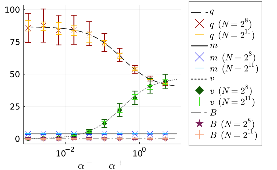
(a) $(\sqrt{\Delta},\lambda)=(1.5,10^{-5})$

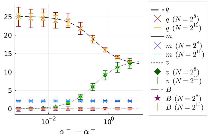
(b) $(\sqrt{\Delta},\lambda)=(1.5,10^{-3})$

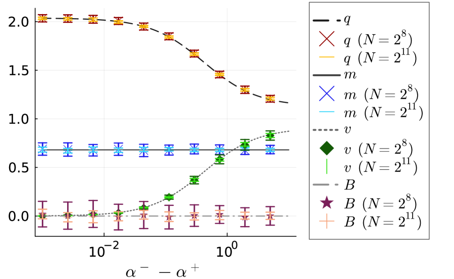
(c) $(\sqrt{\Delta},\lambda)=(1.5,10^{-1})$

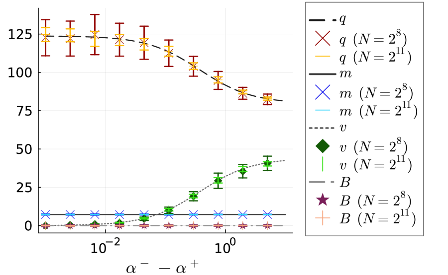
(d) $(\sqrt{\Delta},\lambda)=(0.75,10^{-5})$

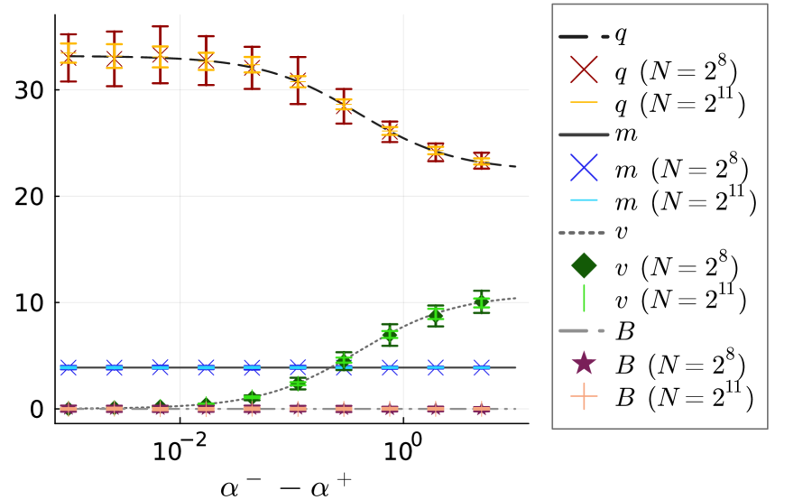
(e) $(\sqrt{\Delta},\lambda)=(0.75,10^{-3})$

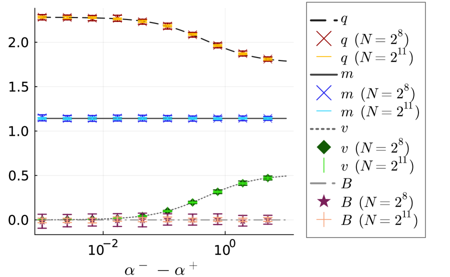
(f) $(\sqrt{\Delta},\lambda)=(0.75,10^{-1})$

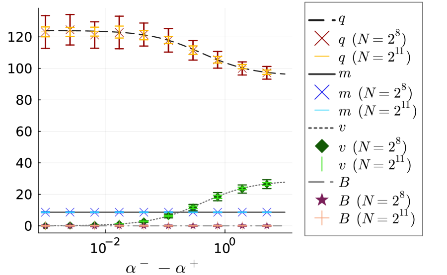
(g) $(\sqrt{\Delta},\lambda)=(0.5,10^{-5})$

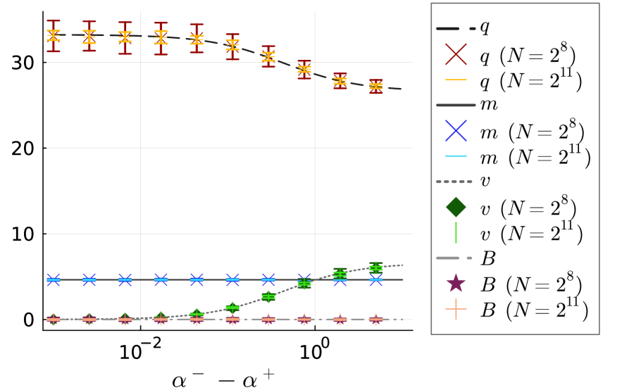
(h) $(\sqrt{\Delta},\lambda)=(0.5,10^{-3})$

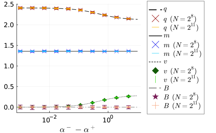
(i) $(\sqrt{\Delta},\lambda)=(0.5,10^{-1})$

Figure 2: Comparison of the comparison of $(q,m,v,B)$, obtained as the solution of the self-consistent equation (lines), and $(N^{-1}\sum_{i}\mathbb{E}_{\mathbf{\boldsymbol{c}}}[\hat{w}_{i}(\mathbf{\boldsymbol{c}},D)]^{2},N^{-1}\sum_{i}\mathbb{E}_{\mathbf{\boldsymbol{c}}}[\hat{w}_{i}(\mathbf{\boldsymbol{c}},D)],N^{-1}\sum_{i}{\mathbb{V}}_{\mathbf{\boldsymbol{c}}}[\hat{w}_{i}(\mathbf{\boldsymbol{c}},D)],\hat{B}(\mathbf{\boldsymbol{c}},D))$ (markers with error bars). Reported experimental results are averaged over several realization of $D$ depending on the size $N$. The error bars represent standard deviations. Each panel corresponds to different values of $(\Delta,\lambda)$. Different colors of the lines represent the result for different system sizes $N$.

Parameters $\Theta$

Figure 2 shows the comparison of $(q,m,v,B)$, obtained as the solution of the self-consistent equation, and $(N^{-1}\sum_{i}\mathbb{E}_{\mathbf{\boldsymbol{c}}}[\hat{w}_{i}(\mathbf{\boldsymbol{c}},D)]^{2},N^{-1}\sum_{i}\mathbb{E}_{\mathbf{\boldsymbol{c}}}[\hat{w}_{i}(\mathbf{\boldsymbol{c}},D)],N^{-1}\sum_{i}{\mathbb{V}}_{\mathbf{\boldsymbol{c}}}[\hat{w}_{i}(\mathbf{\boldsymbol{c}},D)],\hat{B}(\mathbf{\boldsymbol{c}},D))$. The values are plotted as functions of $\alpha^{-}-\alpha^{+}$, the difference of the normalized size of the majority and the minority classes. Each panel corresponds to a different set of $(\lambda,\sqrt{\Delta})$. For numerical experiments, two different system sizes $N=256(=2^{8})$, and $2048(=2^{11})$ are used. To take the average over $\mathbf{\boldsymbol{c}}$, $128$ independent realizations are used. Reported experimental results are averaged over several realization of $D$ depending on the size $N$. The results show that the theoretical predictions and the experimental values are in good agreement. Also, the error bars represent standard deviations that decrease as the system size grows, indicating the concentration of these quantities. Overall, the figure confirms the validity of Claim 1 and Assumption 1.

4 Under-bagging and regularization

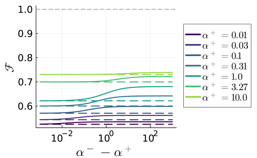
(a) $(\sqrt{\Delta},\lambda)=(1.5,10^{-3})$

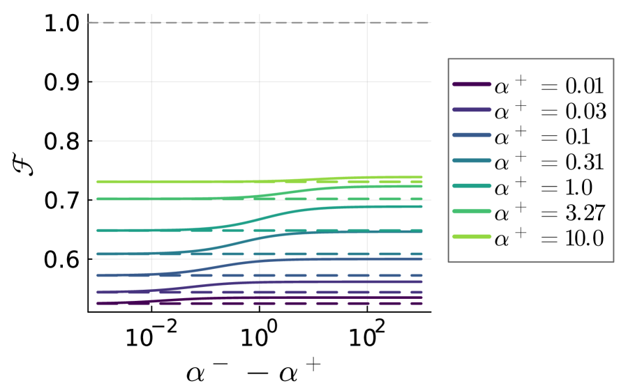
(b) $(\sqrt{\Delta},\lambda)=(1.5,10^{-1})$

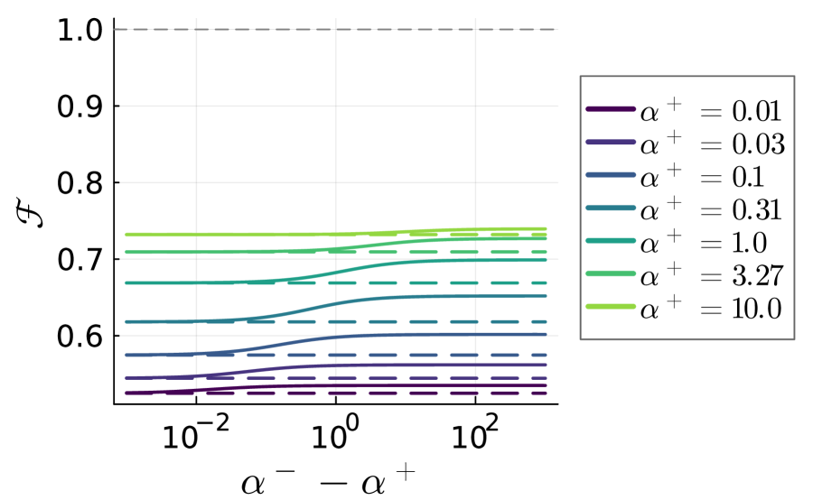
(c) $(\sqrt{\Delta},\lambda)=(1.5,10^{0})$

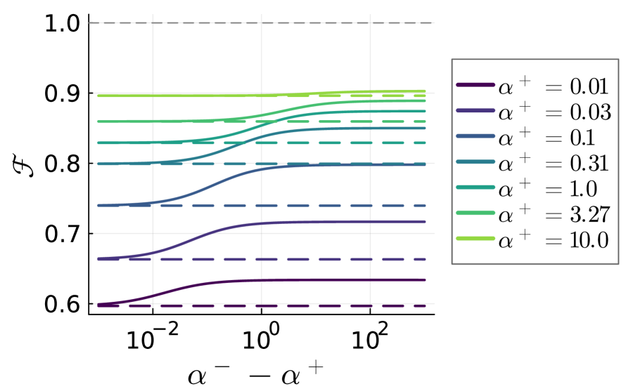
(d) $(\sqrt{\Delta},\lambda)=(0.75,10^{-3})$

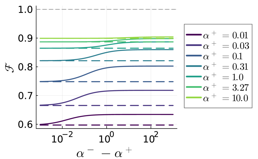
(e) $(\sqrt{\Delta},\lambda)=(0.75,10^{-1})$

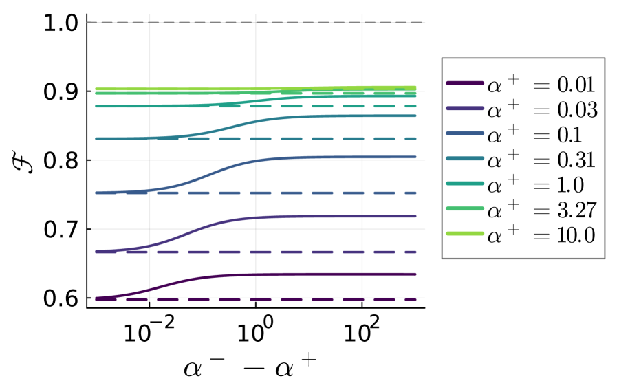
(f) $(\sqrt{\Delta},\lambda)=(0.75,10^{0})$

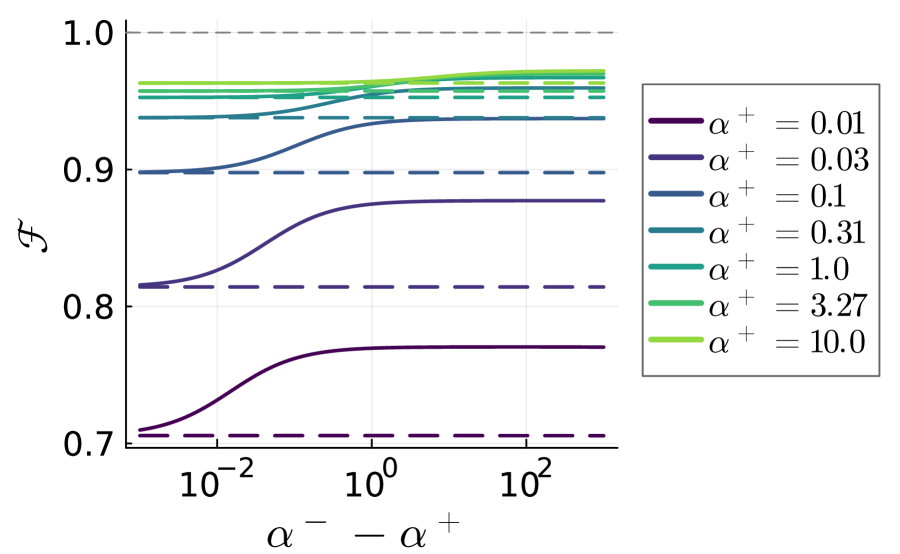
(g) $(\sqrt{\Delta},\lambda)=(0.5,10^{-3})$

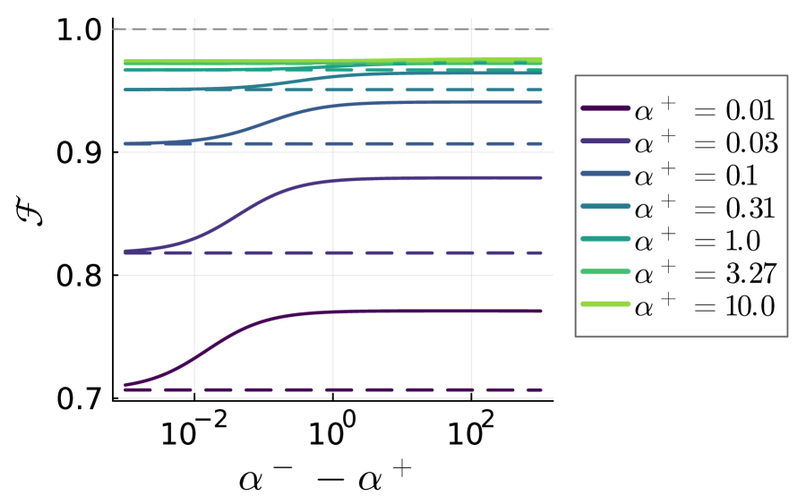
(h) $(\sqrt{\Delta},\lambda)=(0.5,10^{-1})$

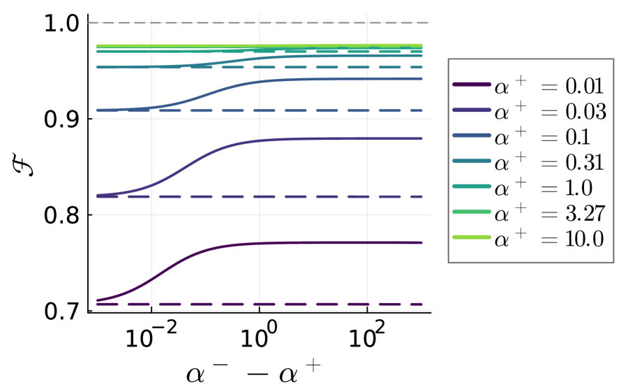
(i) $(\sqrt{\Delta},\lambda)=(0.5,10^{0})$

Figure 3: Comparison of the dependence of the $F$-measure ${\mathcal{F}}$ on $\alpha^{-}-\alpha^{+}$, which is the difference in the size between the majority (negative) and the minority (positive) classes, between US (dashed) and UB (solid). Each panel corresponds to different values of $(\Delta,\lambda)$. Different colors of the lines represent the result for different sizes of the minority classes $\alpha^{+}$.

In this section, using Claim 4, we compare the performance of several estimators, that is, US, UB, and SW.

For simplicity, we focus on the case of ridge-regularized cross-entropy loss as in subsection 3.1. When training a model using an under-sampled data set as in (6)-(7), we can expect that the estimated bias term $\hat{B}(\mathbf{\boldsymbol{c}},D)$ to be zero, since the number of positive and negative samples is balanced. See also Figure 2. Therefore, we set the bias to zero a priori when using subsampled data sets. Furthermore, as investigated in the previous studies (Dobriban & Wager, 2018; Mignacco et al., 2020), when training a linear classifier using balanced data and a ridge-regularized cross-entropy loss, an infinitely large regularization parameter yields the best direction for the classification plane. However, as reported in (Mignacco et al., 2020; Takahashi, 2024), the discrepancy between the theory and experiment with finite $N$ can be huge if too a large regularization parameter is used because the norm of the weight vector can be pathologically small. Therefore, for US and UB, we consider several finite and fixed regularization parameters. When considering the weighting, the behavior of the bias and the optimal regularization parameter is not known a priori. Hence the bias term is estimated as in (4) and the regularization parameter is optimized to maximize the $F$-measure using the Nelder-Mead method in Optim.jl package (Mogensen & Riseth, 2018).

4.1 US and UB

In this subsection, we compare the performance of US and UB, through the values of $F$-measures.

Figure 3 shows the dependence of the $F$-measure ${\mathcal{F}}$ on $\alpha^{-}-\alpha^{+}$, which is the difference in the scaled size between the majority (negative) and minority (positive) classes, or equivalently, the scaled size of the excess majority examples. Each panel corresponds to different values of the variance $\Delta$ and the regularization parameter $\lambda$. Recall that the $F$-measure is uppder bounded by unity. In UB, the $F$-measure increases monotonically as the number of excess data points in the majority class $\alpha^{-}-\alpha^{+}$ increases, despite of the large class imbalance. However, in the case of US, the $F$-measure does not depends on $\alpha^{-}-\alpha^{+}$, i.e., it is not affected by the class imbalance, but cannot utilize the excess data points in the majority class. This tendency does not depend on the values of $(\Delta,\lambda)$. Actually, when subsampling is used as the resampling method, one can show that the performance of the classifier does not depends on $\alpha^{-}-\alpha^{+}$ as shown below.

The $F$-measure for the estimator obtained by US, which corresponds to the case of $K=1$ in Claim 4, is determined by $\bar{q}=q+v$. Let us also define $\hat{\bar{\chi}}=\hat{\chi}+\hat{v}$. Then, by adding both side of equations (18) and (20) as well as (22) and (24), and taking the average of $c^{\pm}\sim p_{c}^{\pm}$ explicitly, the following modified self-consistent equations that determine $\bar{q},m,B$ are obtained as follows.

Claim 5 (Modified self-consistent equations for US)

Let $\bar{q}=q+v$ and $\hat{\bar{\chi}}=\hat{\chi}+\hat{v}$. Then, the set of quantities $\bar{q},m,\chi$ and $\hat{Q},\hat{\bar{\chi}},\hat{m}$ are given as the solution of the following set of modified self-consistent equations when subsampling (6)-(7) is used for the resampling method. Let $\bar{\mathsf{w}}$ and $\bar{\mathsf{u}}^{\pm}$ be the solution of the following one-dimensional randomized optimization problems:

$$\bar{\mathsf{w}} =\operatorname*{arg\,min}_{w\in\mathbb{R}}\frac{\hat{Q}}{2}w^{2}-\bar{h}_{w}w+\lambda r(w),$$ (38)

$$\bar{\mathsf{u}}^{\pm} =\operatorname*{arg\,min}_{u\in\mathbb{R}}\frac{u^{2}}{2\chi\Delta}+l^{\pm}(u+\bar{h}_{u}^{\pm}),$$ (39)

where

$$\bar{h}_{w} =\hat{m}+\sqrt{\hat{\bar{\chi}}}\xi_{w},\quad\xi_{w},\sim{\mathcal{N}}(0,1),$$ (40)

$$\bar{h}_{u}^{\pm} =B\pm m+\sqrt{\bar{q}}\xi_{u},\quad\xi_{u}\sim{\mathcal{N}}(0,\Delta).$$ (41)

Then, the modified self-consistent equations are given as follows:

$$\chi =E_{\xi_{w},\sim{\mathcal{N}}(0,1)}\left[\frac{d}{d\bar{h}_{w}}\bar{\mathsf{w}}\right],$$ (42)

$$\bar{q} =\mathbb{E}_{\xi_{w}\sim{\mathcal{N}}(0,1)}\left[\bar{\mathsf{w}}^{2}\right],$$ (43)

$$m =E_{\xi_{w}\sim{\mathcal{N}}(0,1)}\left[\bar{\mathsf{w}}\right],$$ (44)

$$\hat{Q} =-\frac{\alpha^{+}}{\chi}\mathbb{E}_{\xi_{u}\sim{\mathcal{N}}(0,\Delta)}\left[\frac{d}{d\bar{h}_{u}^{+}}\bar{\mathsf{u}}^{+}+\frac{d}{d\bar{h}_{u}^{-}}\bar{\mathsf{u}}^{-}\right],$$ (45)

$$\hat{\bar{\chi}} =\frac{\alpha^{+}}{\Delta\chi^{2}}\mathbb{E}_{\xi_{u}\sim{\mathcal{N}}(0,\Delta)}\left[(\bar{\mathsf{u}}^{+})^{2}+(\bar{\mathsf{u}}^{-})^{2}\right],$$ (46)

$$\hat{m} =\frac{\alpha^{+}}{\Delta\chi}\mathbb{E}_{\xi_{u},\sim{\mathcal{N}}(0,\Delta)}\left[\bar{\mathsf{u}}^{+}-\bar{\mathsf{u}}^{-}\right].$$ (47)

Furthermore, depending on whether the bias is estimated or fixed, the following equation is added to the modified self-consistent equation

$$\begin{cases}0=\mathbb{E}_{\xi_{u}\sim{\mathcal{N}}(0,\Delta)}\left[\bar{\mathsf{u}}^{+}+\bar{\mathsf{u}}^{-}\right],&{\rm when~{}bias~{}is~{}estimated\vspace{2truemm}}\\ B=\bar{B},&{\rm when~{}bias~{}is~{}fixed}\end{cases}.$$ (48)

It is clear that the above modified self-consistent equation only depends on $\alpha^{+}$ and does not depends on $\alpha^{-}-\alpha^{+}$. Therefore, the $F$-measure of US cannot be improved by the excess examples the majority class.

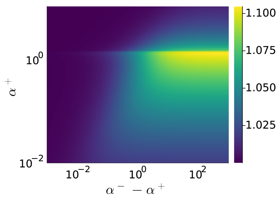
(a) $(\sqrt{\Delta},\lambda)=(1.5,10^{-5})$

(b) $(\sqrt{\Delta},\lambda)=(1.5,10^{-1})$

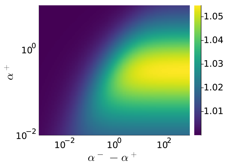
(c) $(\sqrt{\Delta},\lambda)=(1.5,10^{0})$

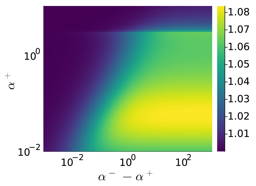
(d) $(\sqrt{\Delta},\lambda)=(0.75,10^{-5})$

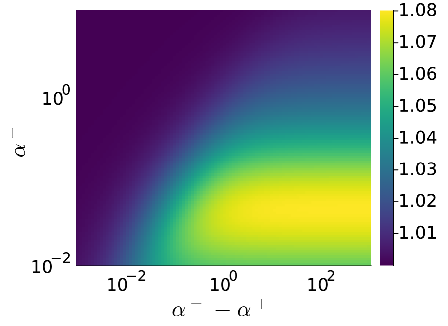
(e) $(\sqrt{\Delta},\lambda)=(0.75,10^{-1})$

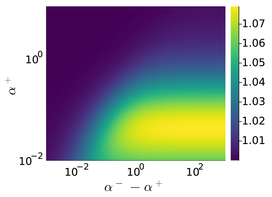
(f) $(\sqrt{\Delta},\lambda)=(0.75,10^{0})$

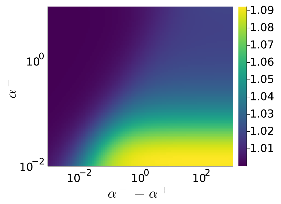
(g) $(\sqrt{\Delta},\lambda)=(0.5,10^{-5})$

(h) $(\sqrt{\Delta},\lambda)=(0.5,10^{-1})$

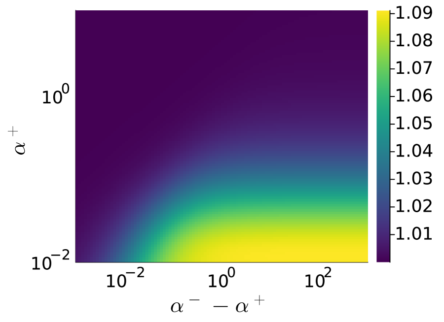
(i) $(\sqrt{\Delta},\lambda)=(0.5,10^{0})$

Figure 4: Heatmap plot for the relative $F$-measure ${\mathcal{F}}_{\rm UB}/{\mathcal{F}}_{\rm US}$, where ${\mathcal{F}}_{\rm UB}$ and ${\mathcal{F}}_{\rm US}$ are the $F$-measure for UB and US, respectively. Each panel corresponds to different values of $(\Delta,\lambda)$.

Figure 4 shows heatmap of the relative $F$-measure ${\mathcal{F}}_{\rm UB}/{\mathcal{F}}_{\rm US}$, where ${\mathcal{F}}_{\rm UB}$ and ${\mathcal{F}}_{\rm US}$ are the $F$-measure for UB and US, respectively. It is clear that the values of the $F$-measures are improved when the variance is small, the size of the minority class is small and the excess size of the majority class is large. When the variance is large, the improvement at extremely small $\alpha^{+}$ region is small because $m$ in (36) can be small due to the large overlap between two clusters.

4.1.1 Double-descent-like behavior

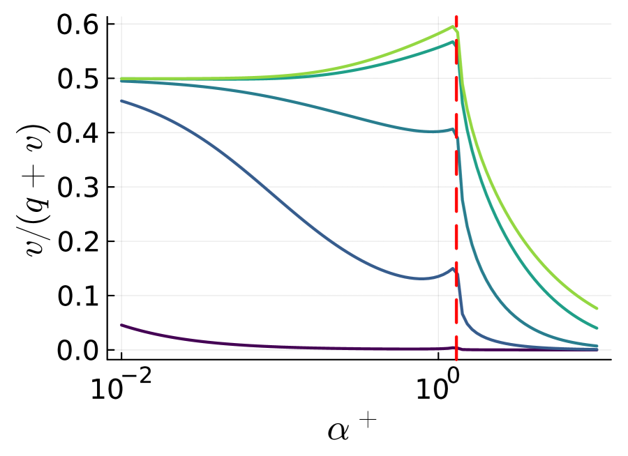
(a) $(\sqrt{\Delta},\lambda)=(1.5,10^{-5})$

(b) $(\sqrt{\Delta},\lambda)=(0.75,10^{-5})$

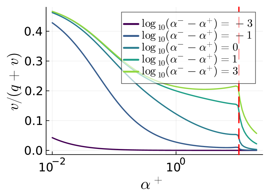
(c) $(\sqrt{\Delta},\lambda)=(0.5,10^{-5})$

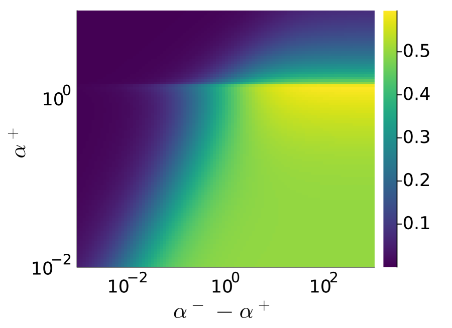
(d) $(\sqrt{\Delta},\lambda)=(1.5,10^{-5})$

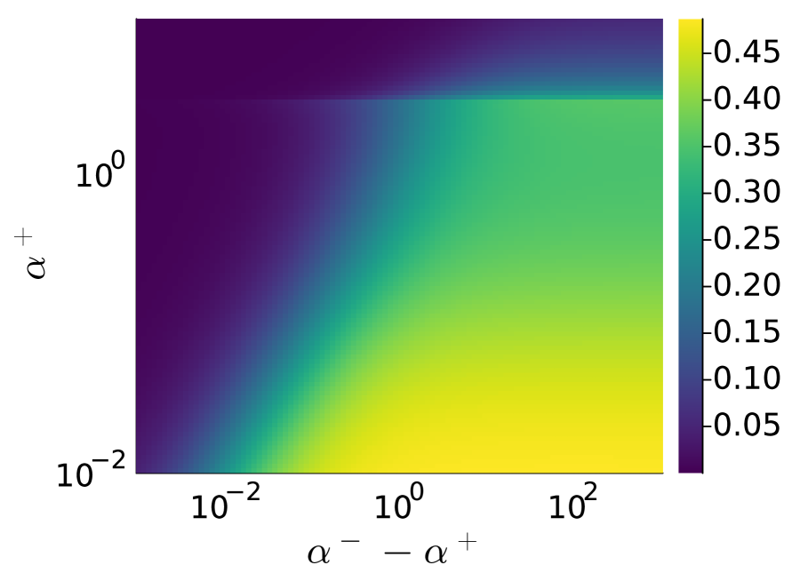
(e) $(\sqrt{\Delta},\lambda)=(0.75,10^{-5})$

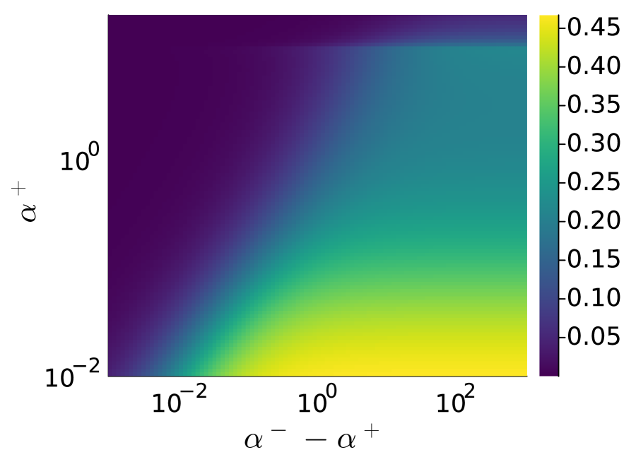
(f) $(\sqrt{\Delta},\lambda)=(0.5,10^{-5})$

Figure 5: Relative variance $v/(q+v)$. Upper panels: the relative variance shown as a function of $\alpha^{+}$ for some selected values of $\alpha^{-}-\alpha^{+}$. The legend is common across all panels. Red dashed lines represent the interpolation threshold. Lower panels: the relative variance shown as a 2d-heatmap.

It is also noteworthy that the improvement may be large around some values of $\alpha^{+}$ when the regularization parameter is extremely small. This is because the variance associated with random reweighting coefficient $\mathbf{\boldsymbol{c}}$ exhibits double-descent-like behavior with respect to $\alpha^{+}$ and takes a large value at a certain $\alpha^{+}$. This point is evident in Figure 5 that shows the relative variance $v/(q+v)$ for several values of $\Delta$. It is clear that the relative variance takes a peak value at the interpolation threshold obtained by the formula in the logistic regression with balanced two-component Gaussian mixture with data size $\alpha^{+}N$ (Mignacco et al., 2020). Similar double-descent-like behavior is also observed in an analysis of bagging without class imbalance structure (Clarté et al., 2024). This indicates that the UB, which can remove the contribution from $v$, is robust to the existence of the phase transition from linearly separable to inseparable training data, although the performance of standard interpolator obtained by a single realization of training data is affected by such a phase transition as reported in (Mignacco et al., 2020).

4.2 UB and SW

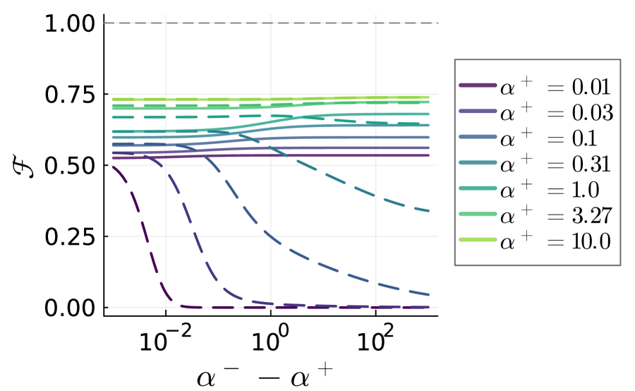
(a) $(\sqrt{\Delta},\lambda)=(1.5,10^{-5})$

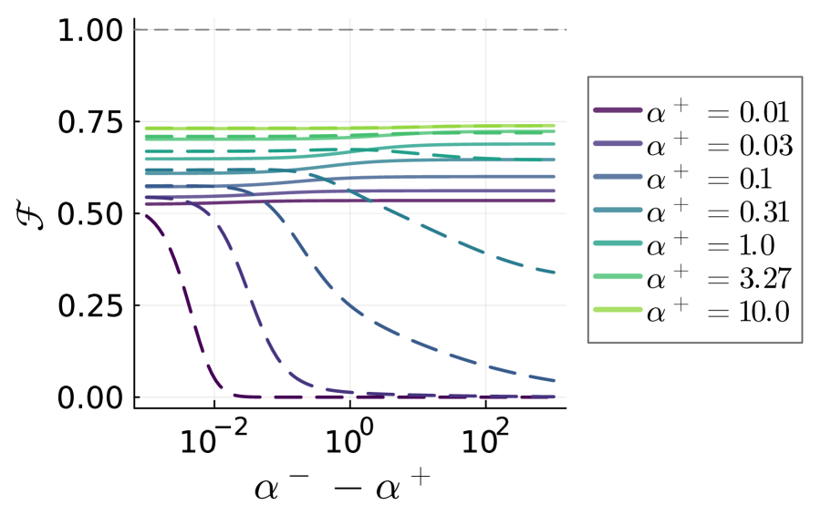
(b) $(\sqrt{\Delta},\lambda)=(1.5,10^{-1})$

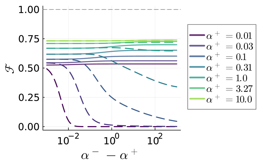
(c) $(\sqrt{\Delta},\lambda)=(1.5,10^{0})$

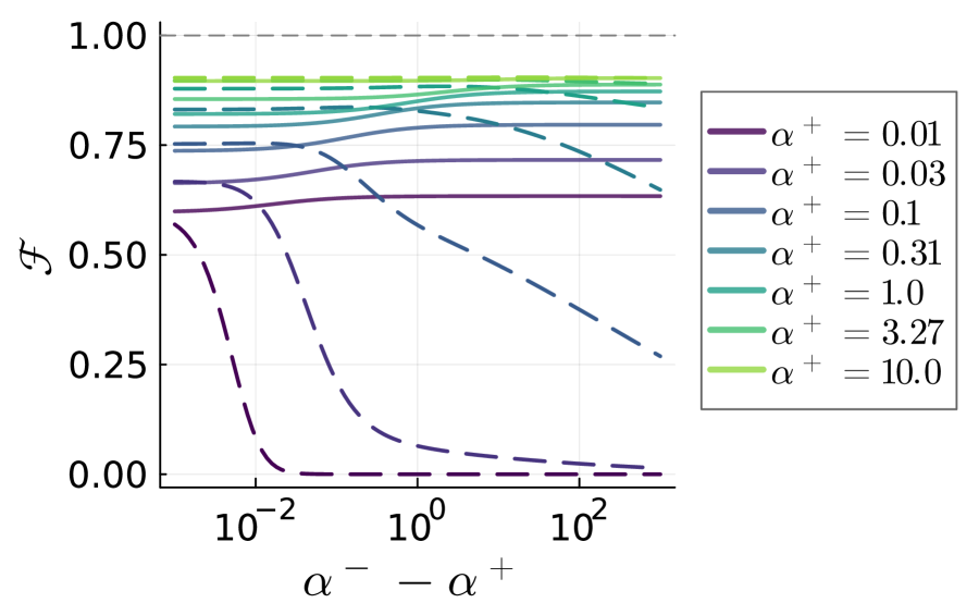
(d) $(\sqrt{\Delta},\lambda)=(0.75,10^{-5})$

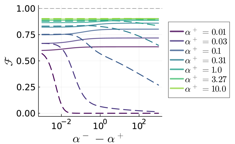
(e) $(\sqrt{\Delta},\lambda)=(0.75,10^{-1})$

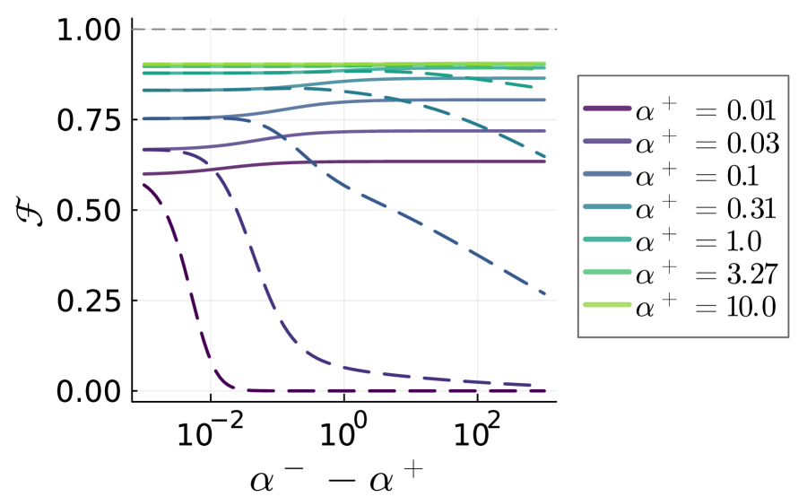
(f) $(\sqrt{\Delta},\lambda)=(0.75,10^{0})$

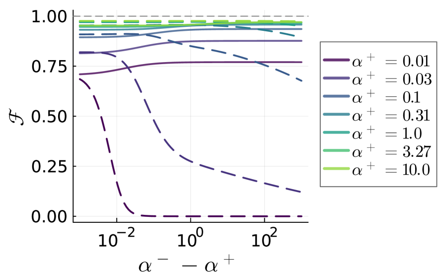
(g) $(\sqrt{\Delta},\lambda)=(0.5,10^{-5})$

(h) $(\sqrt{\Delta},\lambda)=(0.5,10^{-1})$

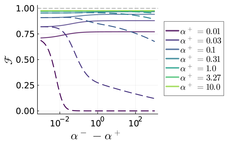
(i) $(\sqrt{\Delta},\lambda)=(0.5,10^{0})$

Figure 6: The comparison of the dependence of the $F$-measure ${\mathcal{F}}$ on $\alpha^{-}-\alpha^{+}$, which is the difference in the size between the majority (negative) and the minority (positive) classes, between weighting (dashed) and UB (solid). Each panel corresponds to different values of $(\Delta,\lambda)$, where $\lambda$ is the regularization parameter for UB. Different colors of the lines represent the result for different sizes of the minority classes $\alpha^{+}$.

In this subsection, we compare the performance of UB with SW, through the values of $F$-measures. For SW, the standard weighting coefficients $\gamma^{+}=M/(2M^{+})=(\alpha^{+}+\alpha^{-})/(2\alpha^{+}),\gamma^{-}=M/(2M^{-})=(\alpha^{+}+\alpha^{-})/(2\alpha^{-})$ are used.

Figure 6 shows the dependence of the $F$-measure ${\mathcal{F}}$ on $\alpha^{-}-\alpha^{+}$, which is the difference in the size between the majority (negative) and minority (positive) classes. In contrast to US and UB, the $F$-measure of the SW method decreases as the number of the excess examples of the majority class increases. In other words, as the amount of the class imbalance increases, the prediction performance of the estimator obtained by simple class-wise weighted cost deteriorates, although the amount of the decrease is mild if the size of the minority class is large. Similarly, Figure 6 shows heatmap of the relative $F$-measure ${\mathcal{F}}_{\rm UB}/{\mathcal{F}}_{\rm SW}$ in a log-scale, where ${\mathcal{F}}_{\rm UB}$ and ${\mathcal{F}}_{\rm SW}$ are the $F$-measure for UB and SW, respectively. When the size of the minority class is sufficiently large, the performance is almost comparable. However, when the size of the minority class is small and the class imbalance is large, the performance of the simple weighting method is several times to tens of thousands of times worser than UB in terms of the value of $F$-measure.

(a) $(\sqrt{\Delta},\lambda)=(1.5,10^{-5})$

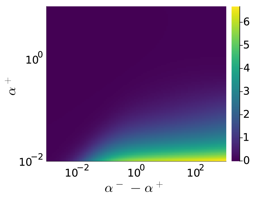
(b) $(\sqrt{\Delta},\lambda)=(1.5,10^{-1})$

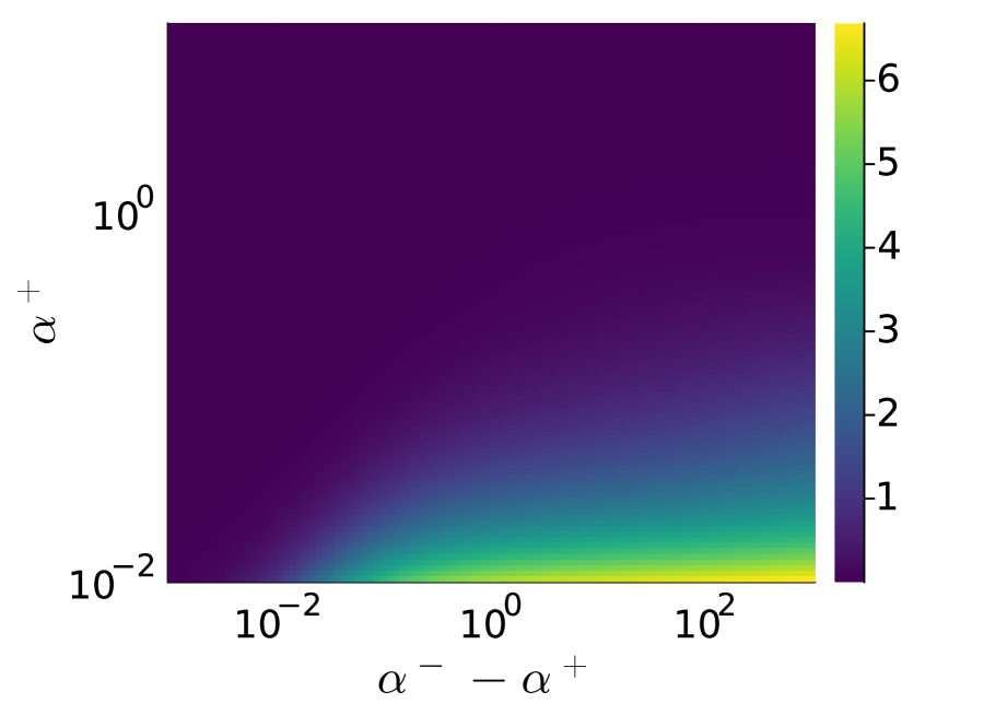
(c) $(\sqrt{\Delta},\lambda)=(1.5,10^{0})$

(d) $(\sqrt{\Delta},\lambda)=(0.75,10^{-5})$

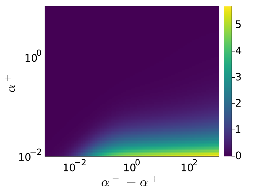
(e) $(\sqrt{\Delta},\lambda)=(0.75,10^{-1})$

(f) $(\sqrt{\Delta},\lambda)=(0.75,10^{0})$

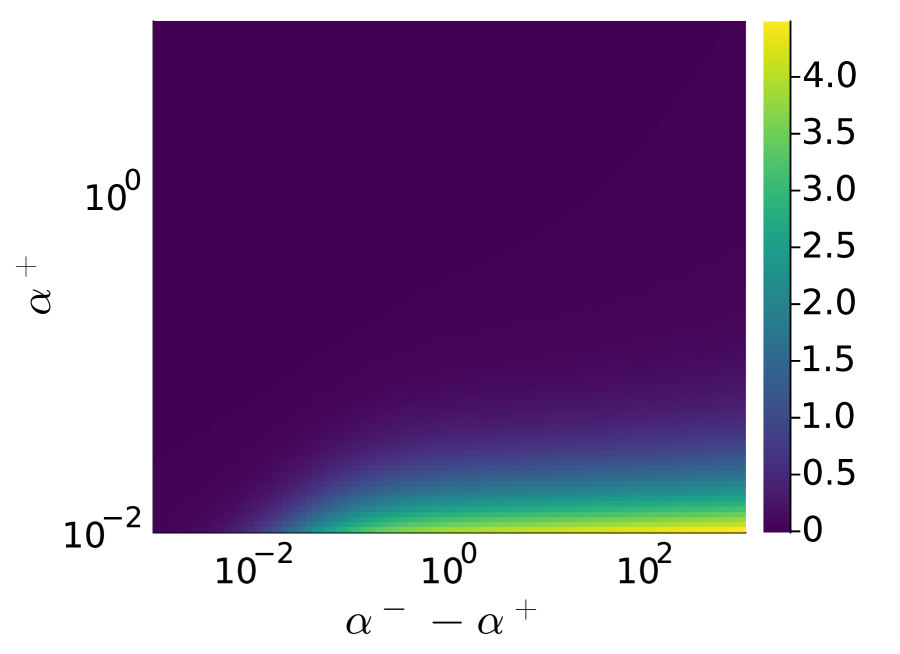
(g) $(\sqrt{\Delta},\lambda)=(0.5,10^{-5})$

(h) $(\sqrt{\Delta},\lambda)=(0.5,10^{-1})$

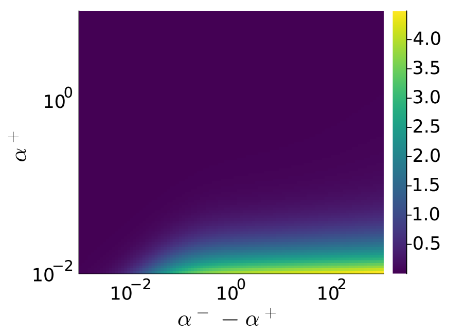
(i) $(\sqrt{\Delta},\lambda)=(0.5,10^{0})$

Figure 7: The heatmap plot for the relative $F$-measure in log-scale: $\log_{10}{\mathcal{F}}_{\rm UB}/{\mathcal{F}}_{\rm weighting}$, where ${\mathcal{F}}_{\rm UB}$ and ${\mathcal{F}}_{\rm weighting}$ are the $F$-measure for UB and the weighting method, respectively. Each panel corresponds to different values of $(\Delta,\lambda)$, where $\lambda$ is the regularization parameter used in UB.

5 Summary and Discussions

In this work, we derived a sharp asymptotics of the estimators obtained by the randomly reweighted losses (4) and (5) in the limit where the data size and the input dimension diverge proportionally. The derivation was based on the standard use of the replica method. The results are summarized in Claim 1-5.

Using the derived sharp asymptotics, we investigated the performance of the UB, US, and SW. Our main findings were (i) UB can improve the performance of the classifier in terms of the $F$-measure by increasing the size of the majority class while keeping the size of the minority class fixed, even when the degree of class imbalance becomes large, (ii) the performance of the classifier obtained by US does not depend on the size of the excess majority examples, and (iii) the performance of the SW method deteriorates as the size of the excess majority examples increases especially when the size of the minority class is small and the class imbalance is large. Furthermore, UB was robust to the interpolation phase transition in contrast to US.

In conclusion, the ensembling considering the class imbalance structure is different from the combination of US and ridge regularization. This result is clearly different from the case of naive bagging in training GLMs without considering the class imbalance structure, where ensembling and ridge regularization give the same performance.

Although UB is a powerful method for learning in imbalanced data, it requires an increased computational cost proportional to the number of under-sampled datasets, which can be a serious problem in learning deep neural networks. Therefore, the development of simple heuristics to achieve similar results as UB would be a promising future direction.

Acknowledgments

This study was supported by JSPS KAKENHI Grant No. 21K21310 and 23K16960, and Grant-in-Aid for Transformative Research Areas (A), “Foundation of Machine Learning Physics” (22H05117).

Appendix A Derivation

In this appendix, we outline the derivations of Claim 2. The derivation is based on the standard use of the replica method of statistical physics (Mézard et al., 1987; Charbonneau et al., 2023; Montanari & Sen, 2024). For a pedagogical introduction to the replica method computation for the linear models, see literature (Krzakala & Zdeborová, 2021), for example.

A.1 Additional notations

To describe the derivations, we use some additional shorthand notations. We summarize them in Table 2.

Notation	Description
$\mathop{\rm extr}_{x}f(x)$	extremization with respect to $x$
$d\mathbf{\boldsymbol{x}}$	with $\mathbf{\boldsymbol{x}}\in\mathbb{R}^{N}$, a measure over $\mathbb{R}^{N}$
$d^{n}\mathbf{\boldsymbol{x}}$	with $\mathbf{\boldsymbol{x}}_{1},\dots,\mathbf{\boldsymbol{x}}_{n}\in\mathbb{R}^{N}$, a measure over $\mathbb{R}^{N\times n}$
$I_{N}$	identity matrix of size $N\times N$
$\partial^{k}{\mathcal{F}}(y)$	for a function ${\mathcal{F}}(x)$ and integer $k$,
	the partial derivative of ${\mathcal{F}}$ with respect to its argument at $x=y$: $\left.\frac{\partial^{k}{\mathcal{F}}(x)}{\partial x^{k}}\right|_{x=y}$
$f(n)=\mathcal{O}(g(n))$	Landau’s O as $n\to 0$; $|f(n)/g(n)|<\infty$ as $n\to 0$

Table 2: Additional notations used in the appendix

A.2 Boltzmann distribution

Let us starting with rewriting the training (4)-(5) as a statistical physics problem. For this, we introduce a probability density function $p_{\rm B}$, which is termed the Boltzmann distribution, as follows. Let ${\mathcal{L}}(\mathbf{\boldsymbol{\theta}};D,\mathbf{\boldsymbol{c}})$ be the cost function to be optimized in (4)-(5). Then, the Boltzmann distribution is defined as

$$p_{\rm B}(\mathbf{\boldsymbol{\theta}}|D,\mathbf{\boldsymbol{c}})=\frac{1}{Z(D,\mathbf{\boldsymbol{c}})}e^{-\beta{\mathcal{L}}(\mathbf{\boldsymbol{\theta}};D,\mathbf{\boldsymbol{c}})},$$ (49)

where $\beta\in(0,\infty)$ is the positive parameter termed the inverse temperature following the custom of statistical physics, and $Z(D,\mathbf{\boldsymbol{c}})=\int e^{-\beta{\mathcal{L}}(\mathbf{\boldsymbol{\theta}};D,\mathbf{\boldsymbol{c}})}d\mathbf{\boldsymbol{\theta}}$ is the normalization constant. For simplicity, we use the same notation for the model’s parameter whether the bias is fixed or not. We basically consider the case when the bias is estimated, but just replace $B$ with $\bar{B}$ when the bias is fixed.

At $\beta\to\infty$, the Boltzmann distribution converges to the uniform distribution over the minimum of ${\mathcal{L}}(\mathbf{\boldsymbol{\theta}};D,\mathbf{\boldsymbol{c}})$. Since we are considering a convex loss function, the Boltzmann distribution converges to the Delta function at $\beta\to\infty$:

$$\lim_{\beta\to\infty}p_{\rm B}(\mathbf{\boldsymbol{\theta}}|D,\mathbf{\boldsymbol{c}})=\delta_{\rm d}(\mathbf{\boldsymbol{\theta}}-\hat{\mathbf{\boldsymbol{\theta}}}(D,\mathbf{\boldsymbol{c}})).$$ (50)

Therefore, analyzing the Boltzmann distribution at this limit is equivalent to analyzing the estimators defined in (4)-(5).

A.3 Distribution of the prediction

In the following, we use the replica method to consider the distribution of the prediction for a new input.

A.3.1 Replicated system

We are interested in how the prediction for a new input $\hat{s}^{\pm}(\mathbf{\boldsymbol{c}},D)\equiv\mathbf{\boldsymbol{x}}^{\pm}\cdot\hat{\mathbf{\boldsymbol{w}}}(\mathbf{\boldsymbol{c}},D)/\sqrt{N}+\hat{B}(\mathbf{\boldsymbol{c}},D)$ depends on $\mathbf{\boldsymbol{x}}$ and $\mathbf{\boldsymbol{c}}$. For this, we introduce another probability density, which we refer to as the replciated system, as follows. Let $n_{1},n_{2}\in{\mathbb{N}}$ be the positive integers. Then, the replicated system is defined as follows:

$$\tilde{p}(\{\mathbf{\boldsymbol{\theta}}_{\mathbf{\boldsymbol{a}}}\})=\frac{1}{\Xi}\mathbb{E}_{D}\left[\prod_{a_{1}=1}^{n_{1}}\mathbb{E}_{\mathbf{\boldsymbol{c}}_{a_{1}}\sim p_{c}}\left[\prod_{a_{2}=1}^{n_{2}}e^{-\beta{\mathcal{L}}(\mathbf{\boldsymbol{\theta}}_{\mathbf{\boldsymbol{a}}};D,\mathbf{\boldsymbol{c}}_{a_{1}})}\right]\right],$$ (51)

where $\mathbf{\boldsymbol{a}}=(a_{1}a_{2})$ is the shorthand notation for the subscript, and $\Xi$ is the normalization constant. This is the density over $\mathbb{R}^{(N+1)\times(n_{1}\times n_{2})}$ if the bias is trained and $\mathbb{R}^{N\times(n_{1}\times n_{2})}$ if the bias is fixed. Recall that the replicated system is not conditioned by $D$ or $\mathbf{\boldsymbol{c}}$ since the average is taken explicitly.

Let $l=1,2,\dots$ be the positive integer, and take $n_{1}>l$. Also, let $\mathbf{\boldsymbol{a}}^{(1)}=(a_{1}^{(1)}a_{2}^{(1)}),\dots,\mathbf{\boldsymbol{a}}^{(l)}=(a_{1}^{(l)}a_{2}^{(l)})$ be a set of indices such that $a_{1}^{(k)}\neq a_{1}^{(k^{\prime})}$ for any $k\neq k^{\prime}\in[l]$. Then, for an arbitrary function $\psi(\cdot)$ such that subsequent integrals converge, we consider the following expectation:

$$\Omega_{l,n_{1},n_{2}}^{\pm}\equiv\mathbb{E}_{\{\mathbf{\boldsymbol{\theta}}_{\mathbf{\boldsymbol{a}}}\}\sim\tilde{p},\mathbf{\boldsymbol{x}}^{\pm}}\left[\prod_{k=1}^{l}\psi(\mathbf{\boldsymbol{x}}^{\pm}\cdot\mathbf{\boldsymbol{w}}_{\mathbf{\boldsymbol{a}}^{(k)}}/\sqrt{N}+B_{\mathbf{\boldsymbol{a}}^{(k)}})\right].$$ (52)

By formally taking the integral with respect to $\{\mathbf{\boldsymbol{\theta}}_{\mathbf{\boldsymbol{a}}}\}$, we obtain the following:

$$\Omega_{l,n_{1},n_{2}}^{\pm}=\frac{1}{\mathbb{E}_{D}\left[\mathbb{E}_{\mathbf{\boldsymbol{c}}}[Z(D,\mathbf{\boldsymbol{c}})^{n_{2}}]^{n_{1}}\right]}\mathbb{E}_{D,\mathbf{\boldsymbol{x}}^{\pm}}\left[\mathbb{E}_{\mathbf{\boldsymbol{c}}}\left[\mathbb{E}_{\mathbf{\boldsymbol{\theta}}\sim p_{\rm B}}\left[\psi(\mathbf{\boldsymbol{x}}^{\pm}\cdot\mathbf{\boldsymbol{w}}/\sqrt{N}+B)\right]Z(D,\mathbf{\boldsymbol{c}})^{n_{2}}\right]^{l}\mathbb{E}_{\mathbf{\boldsymbol{c}}}\left[Z(D,\mathbf{\boldsymbol{c}})^{n_{2}}\right]^{n_{1}-l}\right].$$ (53)

Since the above expression depends on $n_{1}$ and $n_{2}$ in the form of the power function, we can consider formal analytical continuation of $n_{1},n_{2}\in{\mathbb{N}}$ to $n_{1},n_{2}\in\mathbb{R}$, and take the limit $n_{1},n_{2}\to 0$. Then, we obtain the following expression:

$$\lim_{n_{1},n_{2}\to 0}\Omega_{l,n_{1},n_{2}}^{\pm}=\mathbb{E}_{D,\mathbf{\boldsymbol{x}}^{\pm}}\left[\mathbb{E}_{\mathbf{\boldsymbol{c}}}\left[\mathbb{E}_{\mathbf{\boldsymbol{\theta}}\sim p_{\rm B}}\left[\psi(\mathbf{\boldsymbol{x}}^{\pm}\cdot\mathbf{\boldsymbol{w}}/\sqrt{N}+B)\right]\right]^{l}\right].$$ (54)

At the limit $\beta\to\infty$, the above converges to the following:

$$\lim_{\beta\to\infty}\lim_{n_{1},n_{2}\to 0}\Omega_{l,n_{1},n_{2}}^{\pm}=\mathbb{E}_{D,\mathbf{\boldsymbol{x}}^{\pm}}\left[\mathbb{E}_{\mathbf{\boldsymbol{c}}}\left[\psi(\mathbf{\boldsymbol{x}}\cdot\hat{\mathbf{\boldsymbol{w}}}(D,\mathbf{\boldsymbol{c}})/\sqrt{N}+\hat{B}(D,\mathbf{\boldsymbol{c}}))\right]^{l}\right].$$ (55)

Therefore, we can obtain a nontrivial information about the distribution $\hat{s}^{\pm}(\mathbf{\boldsymbol{c}},D)$ if we obtain a nontrivial expression of $\Omega_{l,n_{1},n_{2}}^{\pm}$ and continue the result to $n_{1},n_{2}\in\mathbb{R}$. In the following, we describe the handling of the expectation (52).

A.3.2 Handling of the expectation over the replicated system

Since the normalization constant $\Xi=\mathbb{E}_{D}\left[\mathbb{E}_{\mathbf{\boldsymbol{c}}}[Z(D,\mathbf{\boldsymbol{c}})^{n_{2}}]^{n_{1}}\right]$ just yields the unity at $n_{1},n_{2}\to 0$, we focus on the numerator of the expectation over $\{\mathbf{\boldsymbol{\theta}}_{\mathbf{\boldsymbol{a}}}\}\sim\tilde{p}$ in $\Omega_{l,n_{1},n_{2}}^{\pm}$. Instead of first taking the integral over $\{\mathbf{\boldsymbol{\theta}}_{\mathbf{\boldsymbol{a}}}\}$ as in the computation to obtain (53), we here first consider the average over $\mathbf{\boldsymbol{x}}$ and $D$. Then, using independence of the each data point in $D$ and the reweighting coefficient $\mathbf{\boldsymbol{c}}$, we obtain the following expression of $\Omega_{l,n_{1},n_{2}}^{\pm}$:

$$\Omega_{l,n_{1},n_{2}}^{\pm}\times\Xi= \int\mathbb{E}_{\mathbf{\boldsymbol{z}}}\left[\prod_{k=1}^{l}\psi(\pm\frac{1}{N}\mathbf{\boldsymbol{w}}_{\mathbf{\boldsymbol{a}}^{(k)}}\cdot\mathbf{\boldsymbol{v}}+B_{\mathbf{\boldsymbol{a}}^{(k)}}+\frac{1}{\sqrt{N}}\mathbf{\boldsymbol{w}}_{\mathbf{\boldsymbol{a}}^{(k)}}\cdot\mathbf{\boldsymbol{z}})\right]$$

$$\times\mathbb{E}_{\mathbf{\boldsymbol{z}}^{+},\{c_{a_{1}}^{+}\}}\left[\prod_{\mathbf{\boldsymbol{a}}}e^{-\beta c_{a_{1}}^{+}l^{+}(\frac{1}{N}\mathbf{\boldsymbol{w}}_{\mathbf{\boldsymbol{a}}}\cdot\mathbf{\boldsymbol{v}}+B_{\mathbf{\boldsymbol{a}}}+\frac{1}{\sqrt{N}}\mathbf{\boldsymbol{w}}_{\mathbf{\boldsymbol{a}}}\cdot\mathbf{\boldsymbol{z}}^{+})}\right]^{M^{+}}$$

$$\times\mathbb{E}_{\mathbf{\boldsymbol{z}}^{-},\{c_{a_{1}}^{-}\}}\left[\prod_{\mathbf{\boldsymbol{a}}}e^{-\beta c_{a_{1}}^{-}l^{-}(-\frac{1}{N}\mathbf{\boldsymbol{w}}_{\mathbf{\boldsymbol{a}}}\cdot\mathbf{\boldsymbol{v}}+B_{\mathbf{\boldsymbol{a}}}+\frac{1}{\sqrt{N}}\mathbf{\boldsymbol{w}}_{\mathbf{\boldsymbol{a}}}\cdot\mathbf{\boldsymbol{z}}^{-})}\right]^{M^{-}}\prod_{i=1}^{N}\prod_{\mathbf{\boldsymbol{a}}}e^{-\beta r_{w_{\mathbf{\boldsymbol{a}},i}}}d^{n_{1}n_{2}}\mathbf{\boldsymbol{\theta}},$$ (56)

where $c_{a_{1}}^{+}\sim_{\rm iid}p_{c}^{+},c_{a_{1}}^{-}\sim_{\rm iid}p_{c}^{-},a_{1}\in[n_{1}]$ and $z_{i},z_{i}^{\pm}\sim_{\rm iid}p_{z},i\in[N]$. An important observation is that the noise $\mathbf{\boldsymbol{z}}$ appears only through the form of the scaled inner product with $\mathbf{\boldsymbol{w}}_{\mathbf{\boldsymbol{a}}}$. At $N\gg 1$, such quantity follows the Gaussian distribution for a fixed set of $\{\mathbf{\boldsymbol{w}}_{\mathbf{\boldsymbol{a}}}\}$ due to the central limit theorem. Let us define $\tilde{\mathbf{\boldsymbol{u}}}\in\mathbb{R}^{l}$ and $\mathbf{\boldsymbol{u}}^{\pm}\in R^{n_{1}\times n_{2}}$ as

$$\tilde{u}_{k} =\frac{1}{\sqrt{N}}\mathbf{\boldsymbol{w}}_{\mathbf{\boldsymbol{a}}^{(k)}}\cdot\mathbf{\boldsymbol{z}},$$ (57)

$$u_{\mathbf{\boldsymbol{a}}}^{+} =\frac{1}{\sqrt{N}}\mathbf{\boldsymbol{w}}_{\mathbf{\boldsymbol{a}}}\cdot\mathbf{\boldsymbol{z}}^{+},$$ (58)

$$u_{\mathbf{\boldsymbol{a}}}^{-} =\frac{1}{\sqrt{N}}\mathbf{\boldsymbol{w}}_{\mathbf{\boldsymbol{a}}}\cdot\mathbf{\boldsymbol{z}}^{-}.$$ (59)

Then, these quantities follows the Gaussian distributions as $\tilde{\mathbf{\boldsymbol{u}}}\sim{\mathcal{N}}(0,\tilde{S}),\mathbf{\boldsymbol{u}}^{\pm}\sim{\mathcal{N}}(0,S)$, where the covariance matrices are given as

$$\tilde{S}_{k,k^{\prime}} =\Delta\frac{1}{N}\mathbf{\boldsymbol{w}}_{\mathbf{\boldsymbol{a}}^{(k)}}\cdot\mathbf{\boldsymbol{w}}_{\mathbf{\boldsymbol{a}}^{(k^{\prime})}},$$ (60)

$$S_{\mathbf{\boldsymbol{a}},\mathbf{\boldsymbol{b}}} =\Delta\frac{1}{N}\mathbf{\boldsymbol{w}}_{\mathbf{\boldsymbol{a}}}\cdot\mathbf{\boldsymbol{w}}_{\mathbf{\boldsymbol{b}}}.$$ (61)

Also, the center of the clusters $\mathbf{\boldsymbol{v}}$ only appears through the inner product $\mathbf{\boldsymbol{w}}_{\mathbf{\boldsymbol{a}}}\cdot\mathbf{\boldsymbol{v}}/N$. Thus, the integrand in (56) depends on $\{\mathbf{\boldsymbol{w}}_{\mathbf{\boldsymbol{a}}}\}$ only through their inner products, which capture the geometric relations between the estimators and the centroid of clusters $\mathbf{\boldsymbol{v}}$. We call these quantities as order parameters.

The above observation indicates that the factors regarding the loss function in (56) can be evaluated by Gaussian integrals once the order parameters are fixed. To implement this idea, we insert the trivial identities of the delta functions

$$1 =\prod_{\mathbf{\boldsymbol{a}}\neq\mathbf{\boldsymbol{b}}}\int\delta_{\rm d}(NQ_{\mathbf{\boldsymbol{a}}\mathbf{\boldsymbol{b}}}-\mathbf{\boldsymbol{w}}_{\mathbf{\boldsymbol{a}}}\cdot\mathbf{\boldsymbol{w}}_{b})dQ_{\mathbf{\boldsymbol{a}}\mathbf{\boldsymbol{b}}},$$ (62)

$$1 =\prod_{\mathbf{\boldsymbol{a}}}\int\delta_{\rm d}(Nm_{\mathbf{\boldsymbol{a}}}-\mathbf{\boldsymbol{w}}_{\mathbf{\boldsymbol{a}}}\cdot\mathbf{\boldsymbol{v}})dm_{\mathbf{\boldsymbol{a}}},$$ (63)

into (56). Then $\Omega_{l,n_{1},n_{2}}^{\pm}\times\Xi$ can be rewritten as follows

$$\Omega_{l,n_{1},n_{2}}^{\pm}\times\Xi= \int\mathbb{E}_{\tilde{\mathbf{\boldsymbol{u}}}\sim{\mathcal{N}}(0,\tilde{S})}\left[\prod_{k=1}^{l}\psi(\pm m_{\mathbf{\boldsymbol{a}}^{(k)}}+B_{\mathbf{\boldsymbol{a}}^{(k)}}+\tilde{u}_{k})\right]e^{N\alpha^{+}\varphi^{+}+N\alpha^{-}\varphi^{-}}$$

$$\times\prod_{\mathbf{\boldsymbol{a}}\neq\mathbf{\boldsymbol{b}}}\delta_{\rm d}(NQ_{\mathbf{\boldsymbol{a}}\mathbf{\boldsymbol{b}}}-\mathbf{\boldsymbol{w}}_{\mathbf{\boldsymbol{a}}}\cdot\mathbf{\boldsymbol{w}}_{b})\prod_{\mathbf{\boldsymbol{a}}}\delta_{\rm d}(Nm_{\mathbf{\boldsymbol{a}}}-\mathbf{\boldsymbol{w}}_{\mathbf{\boldsymbol{a}}}\cdot\mathbf{\boldsymbol{v}})\prod_{i=1}^{N}\prod_{\mathbf{\boldsymbol{a}}}e^{-\beta r_{w_{\mathbf{\boldsymbol{a}},i}}}d^{n_{1}n_{2}}\mathbf{\boldsymbol{\theta}}d\Theta,$$ (64)

$$\varphi^{+} =\log\mathbb{E}_{\mathbf{\boldsymbol{u}}^{+}\sim{\mathcal{N}}(0,S),\{c_{a_{1}}^{+}\}}\left[\prod_{\mathbf{\boldsymbol{a}}}e^{-\beta c_{a_{1}}^{+}l^{+}(m_{\mathbf{\boldsymbol{a}}}+B_{\mathbf{\boldsymbol{a}}}+u_{\mathbf{\boldsymbol{a}}}^{+})}\right],$$ (65)

$$\varphi^{-} =\log\mathbb{E}_{\mathbf{\boldsymbol{u}}^{-}\sim{\mathcal{N}}(0,S),\{c_{a_{1}}^{-}\}}\left[\prod_{\mathbf{\boldsymbol{a}}}e^{-\beta c_{a_{1}}^{-}l^{-}(-m_{\mathbf{\boldsymbol{a}}}+B_{\mathbf{\boldsymbol{a}}}+u_{\mathbf{\boldsymbol{a}}}^{-})}\right]$$ (66)

where $\Theta$ is the collection of the variables $\{Q_{\mathbf{\boldsymbol{a}}\mathbf{\boldsymbol{b}}}\},\{m_{\mathbf{\boldsymbol{a}}}\}$. To complete the remaining integrals over $\{\mathbf{\boldsymbol{w}}_{\mathbf{\boldsymbol{a}}}\}$, we use the Fourier representations of the delta functions:

$$\delta_{\rm d}(NQ_{\mathbf{\boldsymbol{a}}\mathbf{\boldsymbol{b}}}-\mathbf{\boldsymbol{w}}_{\mathbf{\boldsymbol{a}}}\cdot\mathbf{\boldsymbol{w}}_{b}) =\frac{1}{2\pi}\int e^{(NQ_{\mathbf{\boldsymbol{a}}\mathbf{\boldsymbol{b}}}-\mathbf{\boldsymbol{w}}_{\mathbf{\boldsymbol{a}}}\cdot\mathbf{\boldsymbol{w}}_{\mathbf{\boldsymbol{b}}})\tilde{Q}_{\mathbf{\boldsymbol{a}}\mathbf{\boldsymbol{b}}}}d\tilde{Q}_{\mathbf{\boldsymbol{a}}\mathbf{\boldsymbol{b}}},$$ (67)

$$\delta_{\rm d}(Nm_{\mathbf{\boldsymbol{a}}}-\mathbf{\boldsymbol{w}}_{\mathbf{\boldsymbol{a}}}\cdot\mathbf{\boldsymbol{v}}) =\frac{1}{2\pi}\int e^{-(Nm_{\mathbf{\boldsymbol{a}}}-\mathbf{\boldsymbol{w}}\cdot\mathbf{\boldsymbol{v}})\tilde{m}_{\mathbf{\boldsymbol{a}}}}d\tilde{m}_{\mathbf{\boldsymbol{a}}}.$$ (68)

After using these expressions, the integrals over $\{w_{\mathbf{\boldsymbol{a}},i}\}$ can be independently performed for each $i$, leading to the following expression of $\Omega_{l,n_{1},n_{2}}^{\pm}\times\Xi$:

$$\Omega_{l,n_{1},n_{2}}^{\pm}\times\Xi =\int\mathbb{E}_{\tilde{\mathbf{\boldsymbol{u}}}\sim{\mathcal{N}}(0,\tilde{S})}\left[\prod_{k=1}^{l}\psi(\pm m_{\mathbf{\boldsymbol{a}}^{(k)}}+B_{\mathbf{\boldsymbol{a}}^{(k)}}+\tilde{u}_{k})\right]e^{N{\mathcal{G}}(\Theta,\hat{\Theta})}d\Theta d\hat{\Theta},$$ (69)

$${\mathcal{G}}(\Theta,\hat{\Theta}) =\frac{1}{2}\sum_{\mathbf{\boldsymbol{a}},\mathbf{\boldsymbol{b}}}Q_{\mathbf{\boldsymbol{a}}\mathbf{\boldsymbol{b}}}\tilde{Q}_{\mathbf{\boldsymbol{a}}\mathbf{\boldsymbol{b}}}-\sum_{\mathbf{\boldsymbol{a}}}m_{\mathbf{\boldsymbol{a}}}\tilde{m}_{\mathbf{\boldsymbol{a}}}+\alpha^{+}\varphi^{+}+\alpha^{-}\varphi^{-}+\varphi_{w},$$ (70)

$$\varphi_{w} =\log\int e^{-\frac{1}{2}\sum_{\mathbf{\boldsymbol{a}},\mathbf{\boldsymbol{b}}}\tilde{Q}_{\mathbf{\boldsymbol{a}}\mathbf{\boldsymbol{b}}}w_{\mathbf{\boldsymbol{a}}}w_{\mathbf{\boldsymbol{b}}}+\sum_{\mathbf{\boldsymbol{a}}}\tilde{m}_{\mathbf{\boldsymbol{a}}}w_{\mathbf{\boldsymbol{a}}}}\prod_{\mathbf{\boldsymbol{a}}}e^{-\beta r(w_{\mathbf{\boldsymbol{a}}})}d^{n_{1}n_{2}}w,$$ (71)

where $\hat{\Theta}$ is the correction of variables $\{\tilde{Q}_{\mathbf{\boldsymbol{a}}\mathbf{\boldsymbol{b}}}\},\{\tilde{m}_{\mathbf{\boldsymbol{a}}}\}$. At $N\gg 1$, using the saddle point method, it is understood that the integral over $\Theta,\hat{\Theta}$ is dominated at the extremum $\mathop{\rm extr}_{\Theta,\hat{\Theta}}{\mathcal{G}}(\Theta,\hat{\Theta})$. Hence, we obtain

$$\Omega_{l,n_{1},n_{2}}^{\pm}\times\Xi=\mathbb{E}_{\tilde{\mathbf{\boldsymbol{u}}}\sim{\mathcal{N}}(0,\tilde{S})}\left[\prod_{k=1}^{l}\psi(\pm m_{\mathbf{\boldsymbol{a}}^{(k)}}+B_{\mathbf{\boldsymbol{a}}^{(k)}}+\tilde{u}_{k})\right]e^{N{\mathcal{G}}(\Theta,\hat{\Theta})},$$ (72)

where $\Theta,\hat{\Theta}$ is obtained by the extremum condition $\mathop{\rm mathop}_{\Theta,\hat{\Theta}}{\mathcal{G}}(\Theta,\hat{\Theta})$.

At this point, we can obtain the general expression of the extreme condition. Let us define densities $\tilde{p}_{{\rm eff},w}$ and $\tilde{p}_{{\rm eff},s}^{\pm}$ as follows:

$$\tilde{p}_{{\rm eff},w}(\mathbf{\boldsymbol{w}}) =\frac{1}{Z_{{\rm eff},w}}e^{-\frac{1}{2}\sum_{\mathbf{\boldsymbol{a}},\mathbf{\boldsymbol{b}}}\tilde{Q}_{\mathbf{\boldsymbol{a}}\mathbf{\boldsymbol{b}}}w_{\mathbf{\boldsymbol{a}}}w_{\mathbf{\boldsymbol{b}}}+\sum_{\mathbf{\boldsymbol{a}}}\tilde{m}_{\mathbf{\boldsymbol{a}}}w_{\mathbf{\boldsymbol{a}}}}\prod_{\mathbf{\boldsymbol{a}}}e^{-\beta r(w_{\mathbf{\boldsymbol{a}}})},$$ (73)

$$\tilde{p}_{{\rm eff},u}^{\pm}(\mathbf{\boldsymbol{u}}|\{c_{a_{1}}^{\pm}\}) =\frac{1}{Z_{{\rm eff},u}^{\pm}}\prod_{\mathbf{\boldsymbol{a}}}e^{-\beta c_{a_{1}}^{\pm}l^{\pm}(\pm m_{\mathbf{\boldsymbol{a}}}+B_{\mathbf{\boldsymbol{a}}}+u_{\mathbf{\boldsymbol{a}}})}\times{\mathcal{N}}(\mathbf{\boldsymbol{u}};\mathbf{\boldsymbol{0}},\Delta Q),$$ (74)

where $Q=[Q_{\mathbf{\boldsymbol{a}}\mathbf{\boldsymbol{b}}}]\in\mathbb{R}^{n_{1}n_{2}\times n_{1}n_{2}}$. Then, the exremum condition is given as follows:

$$Q_{\mathbf{\boldsymbol{a}}\mathbf{\boldsymbol{b}}} =\mathbb{E}_{\mathbf{\boldsymbol{w}}\sim p_{{\rm eff},w}}\left[w_{\mathbf{\boldsymbol{a}}}w_{\mathbf{\boldsymbol{b}}}\right],$$ (75)

$$m_{\mathbf{\boldsymbol{a}}} =\mathbb{E}_{\mathbf{\boldsymbol{w}}\sim p_{{\rm eff},w}}\left[w_{\mathbf{\boldsymbol{a}}}\right],$$ (76)

$$\tilde{Q}_{\mathbf{\boldsymbol{a}}\mathbf{\boldsymbol{b}}} =-\alpha^{+}\Delta\mathbb{E}_{\{c_{a_{1}}^{+}\}}\left[\mathbb{E}_{\mathbf{\boldsymbol{u}}^{+}\sim p_{{\rm eff},u}^{+}}\left[c_{a_{1}}^{+}c_{b_{1}}^{+}\beta^{2}\partial l^{+}(m_{\mathbf{\boldsymbol{a}}}+B_{\mathbf{\boldsymbol{a}}}+u_{\mathbf{\boldsymbol{a}}})\partial l^{+}(m_{\mathbf{\boldsymbol{b}}}+B_{\mathbf{\boldsymbol{b}}}+u_{\mathbf{\boldsymbol{b}}})\right.\right.$$

$$\hskip 56.9055pt\left.\left.-\beta c_{a_{1}}^{+}\partial^{2}l^{+}(m_{\mathbf{\boldsymbol{a}}}+B_{\mathbf{\boldsymbol{a}}}+u_{\mathbf{\boldsymbol{a}}})\mbox{\rm 1}\mbox{\rm l}(\mathbf{\boldsymbol{a}}=\mathbf{\boldsymbol{b}})\right]\right]$$

$$\hskip 28.45274pt-\alpha^{-}\Delta\mathbb{E}_{\{c_{a_{1}}^{-}\}}\left[\mathbb{E}_{\mathbf{\boldsymbol{u}}^{-}\sim p_{{\rm eff},u}^{-}}\left[c_{a_{1}}^{-}c_{b_{1}}^{-}\beta^{2}\partial l^{-}(-m_{\mathbf{\boldsymbol{a}}}+B_{\mathbf{\boldsymbol{a}}}+u_{\mathbf{\boldsymbol{a}}})\partial l^{-}(-m_{\mathbf{\boldsymbol{b}}}+B_{\mathbf{\boldsymbol{b}}}+u_{\mathbf{\boldsymbol{b}}})\right.\right.$$

$$\hskip 56.9055pt\left.\left.-\beta c_{a_{1}}^{-}\partial^{2}l^{-}(-m_{\mathbf{\boldsymbol{a}}}+B_{\mathbf{\boldsymbol{a}}}+u_{\mathbf{\boldsymbol{a}}})\mbox{\rm 1}\mbox{\rm l}(\mathbf{\boldsymbol{a}}=\mathbf{\boldsymbol{b}})\right]\right],$$ (77)

$$\tilde{m}_{\mathbf{\boldsymbol{a}}} =-\alpha^{+}\mathbb{E}_{\{c_{a_{1}}^{+}\}}\left[\mathbb{E}_{\mathbf{\boldsymbol{u}}^{+}\sim p_{{\rm eff},u}^{+}}\left[\beta c_{a_{1}}^{+}\partial l^{+}(m_{\mathbf{\boldsymbol{a}}}+B_{\mathbf{\boldsymbol{a}}}+u_{\mathbf{\boldsymbol{a}}})\right]\right]$$

$$\hskip 56.9055pt+\alpha^{-}\mathbb{E}_{\{c_{a_{1}}^{-}\}}\left[\mathbb{E}_{\mathbf{\boldsymbol{u}}^{-}\sim p_{{\rm eff},u}^{-}}\left[\beta c_{a_{1}}^{-}\partial l^{-}(-m_{\mathbf{\boldsymbol{a}}}+B_{\mathbf{\boldsymbol{a}}}+u_{\mathbf{\boldsymbol{a}}})\right]\right].$$ (78)

Also, the next is added if the bias is estimated:

$$0 =\alpha^{+}\mathbb{E}_{\{c_{a_{1}}^{+}\}}\left[\mathbb{E}_{\mathbf{\boldsymbol{u}}^{+}\sim p_{{\rm eff},u}^{+}}\left[c_{a_{1}}^{+}\partial l^{+}(m_{\mathbf{\boldsymbol{a}}}+B_{\mathbf{\boldsymbol{a}}}+u_{\mathbf{\boldsymbol{a}}})\right]\right]$$

$$+\alpha^{-}\mathbb{E}_{\{c_{a_{1}}^{-}\}}\left[\mathbb{E}_{\mathbf{\boldsymbol{u}}^{-}\sim p_{{\rm eff},u}^{-}}\left[c_{a_{1}}^{-}\partial l^{-}(-m_{\mathbf{\boldsymbol{a}}}+B_{\mathbf{\boldsymbol{a}}}+u_{\mathbf{\boldsymbol{a}}})\right]\right].$$ (79)

A.3.3 Replica symmetric ansatz

Since ${\mathcal{G}}(\Theta,\hat{\Theta})$ depends on the discrete nature of $n_{1},n_{2}$, we cannot analytically continue the result to $n_{1},n_{2}\in\mathbb{R}$. To make an analytical continuation, the key issue is to identify the correct form of the extreme condition. The choice that reflect the symmetry of the replicated system when $n_{1},n_{2}\in{\mathbb{N}}$ is the following:

$$Q_{\mathbf{\boldsymbol{a}}\mathbf{\boldsymbol{b}}} =q+\mbox{\rm 1}\mbox{\rm l}(a_{1}=b_{1})v+\mbox{\rm 1}\mbox{\rm l}(\mathbf{\boldsymbol{a}}=\mathbf{\boldsymbol{b}})\frac{\chi}{\beta},$$ (80)

$$m_{\mathbf{\boldsymbol{a}}} =m,$$ (81)

$$\tilde{Q}_{\mathbf{\boldsymbol{a}}\mathbf{\boldsymbol{b}}} =-\beta^{2}\hat{\chi}-\mbox{\rm 1}\mbox{\rm l}(a_{1}=b_{1})\beta^{2}\hat{v}+\mbox{\rm 1}\mbox{\rm l}(\mathbf{\boldsymbol{a}}=\mathbf{\boldsymbol{b}})\beta\hat{Q},$$ (82)

$$\tilde{m}_{\mathbf{\boldsymbol{a}}} =\beta\hat{m},$$ (83)

$$B_{\mathbf{\boldsymbol{a}}} =B.$$ (84)

Evaluating the replicated system using this symmetric form of the extremum and analytically continuing as $n_{1},n_{2}\to 0$ is called the replica symmetric (RS) ansatz. When considering the estimation of the linear models with convex loss, it is empirically known that the RS ansatz yields the exact result (Obuchi & Kabashima, 2019; Takahashi & Kabashima, 2020).

Using this symmetric form of the extremum, after simple algebra, one can find that ${\mathcal{G}}$ can be analytically continued to $n_{1},n_{2}\in\mathbb{R}$ and also ${\mathcal{G}}={\mathcal{O}}(n_{1})+{\mathcal{O}}(n_{2})$. Furthermore, the remaining factor $\mathbb{E}_{\tilde{\mathbf{\boldsymbol{u}}}\sim{\mathcal{N}}(0,\tilde{S})}\left[\prod_{k=1}^{l}\psi(\pm m_{\mathbf{\boldsymbol{a}}^{(k)}}+B_{\mathbf{\boldsymbol{a}}^{(k)}}+\tilde{u}_{k})\right]$ can be rewritten as follows

$$\mathbb{E}_{\tilde{\mathbf{\boldsymbol{u}}}\sim{\mathcal{N}}(0,\tilde{S})}\left[\prod_{k=1}^{l}\psi(\pm m_{\mathbf{\boldsymbol{a}}^{(k)}}+B_{\mathbf{\boldsymbol{a}}^{(k)}}+\tilde{u}_{k})\right]=\mathbb{E}_{\xi_{u}\sim{\mathcal{N}}(0,\Delta)}\left[\mathbb{E}_{\eta_{u}\sim{\mathcal{N}}(0,\Delta)}\left[\psi(\pm m+B+\sqrt{q}\xi_{u}+\sqrt{v}\eta_{u})\right]^{l}\right].$$ (85)

After all, we obtain the following result:

$$\lim_{\beta\to\infty}\lim_{n_{1},n_{2}\to 0}\Omega_{l,n_{1},n_{2}}^{\pm}=\mathbb{E}_{\xi_{u}\sim{\mathcal{N}}(0,\Delta)}\left[\mathbb{E}_{\eta_{u}\sim{\mathcal{N}}(0,\Delta)}\left[\psi(\pm m+B+\sqrt{q}\xi_{u}+\sqrt{v}\eta_{u})\right]^{l}\right],$$ (86)

where $m,B,q,v$ are determined by the extreme condition under the RS ansatz at $\beta\to\infty$, which is given as the self-consistent equation in Definition 1. This yields the Claim 2.

Similarly, by considering the expectations such as $\mathbb{E}_{\{\mathbf{\boldsymbol{\theta}}_{\mathbf{\boldsymbol{a}}}\}\sim\tilde{p}}[\mathbf{\boldsymbol{w}}_{\mathbf{\boldsymbol{a}}}^{\top}\mathbf{\boldsymbol{w}}_{\mathbf{\boldsymbol{b}}}/N],\mathbb{E}_{\{\mathbf{\boldsymbol{\theta}}_{\mathbf{\boldsymbol{a}}}\}\sim\tilde{p}}[\mathbf{\boldsymbol{w}}_{\mathbf{\boldsymbol{a}}}^{\top}\mathbf{\boldsymbol{v}}/N],\mathbb{E}_{\{\mathbf{\boldsymbol{\theta}}_{\mathbf{\boldsymbol{a}}}\}\sim\tilde{p}}[B_{\mathbf{\boldsymbol{a}}}]$, one can obtain Claim 1.

References

- Ando & Komaki (2023) Ryo Ando and Fumiyasu Komaki. On high-dimensional asymptotic properties of model averaging estimators. arXiv preprint arXiv:2308.09476, 2023.
- Barbier & Macris (2019) Jean Barbier and Nicolas Macris. The adaptive interpolation method: a simple scheme to prove replica formulas in Bayesian inference. Probability Theory and Related Fields, 174(3):1133–1185, August 2019. ISSN 1432-2064. doi: 10.1007/s00440-018-0879-0. URL https://doi.org/10.1007/s00440-018-0879-0.
- Barbier et al. (2019) Jean Barbier, Florent Krzakala, Nicolas Macris, Léo Miolane, and Lenka Zdeborová. Optimal errors and phase transitions in high-dimensional generalized linear models. Proceedings of the National Academy of Sciences, 116(12):5451–5460, 2019.
- Bellec & Koriyama (2024) Pierre C Bellec and Takuya Koriyama. Asymptotics of resampling without replacement in robust and logistic regression. arXiv preprint arXiv:2404.02070, 2024.
- Breiman (1996) Leo Breiman. Bagging predictors. Machine learning, 24:123–140, 1996.
- Byrd & Lipton (2019) Jonathon Byrd and Zachary Lipton. What is the effect of importance weighting in deep learning? In Kamalika Chaudhuri and Ruslan Salakhutdinov (eds.), Proceedings of the 36th International Conference on Machine Learning, volume 97 of Proceedings of Machine Learning Research, pp. 872–881. PMLR, 09–15 Jun 2019. URL https://proceedings.mlr.press/v97/byrd19a.html.
- Charbonneau et al. (2023) Patrick Charbonneau, Enzo Marinari, Marc Mézard, Giorgio Parisi, Federico Ricci-Tersenghi, Gabriele Sicuro, and Francesco Zamponi. Spin Glass Theory and Far Beyond. WORLD SCIENTIFIC, 2023. doi: 10.1142/13341. URL https://www.worldscientific.com/doi/abs/10.1142/13341.
- Chawla et al. (2002) Nitesh V Chawla, Kevin W Bowyer, Lawrence O Hall, and W Philip Kegelmeyer. Smote: synthetic minority over-sampling technique. Journal of artificial intelligence research, 16:321–357, 2002.
- Clarté et al. (2024) Lucas Clarté, Adrien Vandenbroucque, Guillaume Dalle, Bruno Loureiro, Florent Krzakala, and Lenka Zdeborová. Analysis of bootstrap and subsampling in high-dimensional regularized regression. arXiv preprint arXiv:2402.13622, 2024.
- Cohen et al. (2006) Gilles Cohen, Mélanie Hilario, Hugo Sax, Stéphane Hugonnet, and Antoine Geissbuhler. Learning from imbalanced data in surveillance of nosocomial infection. Artificial Intelligence in Medicine, 37(1):7–18, 2006. ISSN 0933-3657. doi: https://doi.org/10.1016/j.artmed.2005.03.002. URL https://www.sciencedirect.com/science/article/pii/S0933365705000850. Intelligent Data Analysis in Medicine.
- D’Ascoli et al. (2020) Stéphane D’Ascoli, Maria Refinetti, Giulio Biroli, and Florent Krzakala. Double trouble in double descent: Bias and variance(s) in the lazy regime. In Hal Daumé III and Aarti Singh (eds.), Proceedings of the 37th International Conference on Machine Learning, volume 119 of Proceedings of Machine Learning Research, pp. 2280–2290. PMLR, 13–18 Jul 2020. URL https://proceedings.mlr.press/v119/d-ascoli20a.html.
- Dobriban & Wager (2018) Edgar Dobriban and Stefan Wager. High-dimensional asymptotics of prediction: Ridge regression and classification. The Annals of Statistics, 46(1):247–279, 2018. ISSN 00905364, 21688966. URL https://www.jstor.org/stable/26542784.
- Drummond et al. (2003) Chris Drummond, Robert C Holte, et al. C4. 5, class imbalance, and cost sensitivity: why under-sampling beats over-sampling. In Workshop on learning from imbalanced datasets II, 2003.
- Du et al. (2023) Jin-Hong Du, Pratik Patil, and Arun K. Kuchibhotla. Subsample ridge ensembles: Equivalences and generalized cross-validation. In Andreas Krause, Emma Brunskill, Kyunghyun Cho, Barbara Engelhardt, Sivan Sabato, and Jonathan Scarlett (eds.), Proceedings of the 40th International Conference on Machine Learning, volume 202 of Proceedings of Machine Learning Research, pp. 8585–8631. PMLR, 23–29 Jul 2023. URL https://proceedings.mlr.press/v202/du23d.html.
- Engel & Van den Broeck (2001) A. Engel and C. Van den Broeck. Statistical Mechanics of Learning. Cambridge University Press, 2001.
- Feng et al. (2022) Oliver Y. Feng, Ramji Venkataramanan, Cynthia Rush, and Richard J. Samworth. A unifying tutorial on approximate message passing. Foundations and Trends® in Machine Learning, 15(4):335–536, 2022. ISSN 1935-8237. doi: 10.1561/2200000092. URL http://dx.doi.org/10.1561/2200000092.
- Gerace et al. (2020) Federica Gerace, Bruno Loureiro, Florent Krzakala, Marc Mezard, and Lenka Zdeborova. Generalisation error in learning with random features and the hidden manifold model. In Hal Daumé III and Aarti Singh (eds.), Proceedings of the 37th International Conference on Machine Learning, volume 119 of Proceedings of Machine Learning Research, pp. 3452–3462. PMLR, 13–18 Jul 2020. URL https://proceedings.mlr.press/v119/gerace20a.html.
- He & Garcia (2009) Haibo He and Edwardo A. Garcia. Learning from imbalanced data. IEEE Transactions on Knowledge and Data Engineering, 21(9):1263–1284, 2009. doi: 10.1109/TKDE.2008.239.
- Javanmard & Montanari (2014a) Adel Javanmard and Andrea Montanari. Hypothesis testing in high-dimensional regression under the gaussian random design model: Asymptotic theory. IEEE Transactions on Information Theory, 60(10):6522–6554, 2014a. doi: 10.1109/TIT.2014.2343629.
- Javanmard & Montanari (2014b) Adel Javanmard and Andrea Montanari. Confidence intervals and hypothesis testing for high-dimensional regression. Journal of Machine Learning Research, 15(82):2869–2909, 2014b. URL http://jmlr.org/papers/v15/javanmard14a.html.
- Johnson & Khoshgoftaar (2019) Justin M. Johnson and Taghi M. Khoshgoftaar. Survey on deep learning with class imbalance. Journal of Big Data, 6(1):27, March 2019. ISSN 2196-1115. doi: 10.1186/s40537-019-0192-5. URL https://doi.org/10.1186/s40537-019-0192-5.
- Khan et al. (2018) Salman H. Khan, Munawar Hayat, Mohammed Bennamoun, Ferdous A. Sohel, and Roberto Togneri. Cost-sensitive learning of deep feature representations from imbalanced data. IEEE Transactions on Neural Networks and Learning Systems, 29(8):3573–3587, 2018. doi: 10.1109/TNNLS.2017.2732482.
- King & Zeng (2001) Gary King and Langche Zeng. Logistic regression in rare events data. Political Analysis, 9(2):137–163, 2001. doi: 10.1093/oxfordjournals.pan.a004868.
- Kini et al. (2021) Ganesh Ramachandra Kini, Orestis Paraskevas, Samet Oymak, and Christos Thrampoulidis. Label-imbalanced and group-sensitive classification under overparameterization. In M. Ranzato, A. Beygelzimer, Y. Dauphin, P.S. Liang, and J. Wortman Vaughan (eds.), Advances in Neural Information Processing Systems, volume 34, pp. 18970–18983. Curran Associates, Inc., 2021. URL https://proceedings.neurips.cc/paper_files/paper/2021/file/9dfcf16f0adbc5e2a55ef02db36bac7f-Paper.pdf.
- Krogh & Sollich (1997) Anders Krogh and Peter Sollich. Statistical mechanics of ensemble learning. Phys. Rev. E, 55:811–825, Jan 1997. doi: 10.1103/PhysRevE.55.811. URL https://link.aps.org/doi/10.1103/PhysRevE.55.811.
- Krzakala & Zdeborová (2021) Florent Krzakala and Lenka Zdeborová. Statistical physics methods in optimization and machine learning. Notes. pdf, 2021.
- LeJeune et al. (2020) Daniel LeJeune, Hamid Javadi, and Richard Baraniuk. The implicit regularization of ordinary least squares ensembles. In Silvia Chiappa and Roberto Calandra (eds.), Proceedings of the Twenty Third International Conference on Artificial Intelligence and Statistics, volume 108 of Proceedings of Machine Learning Research, pp. 3525–3535. PMLR, 26–28 Aug 2020. URL https://proceedings.mlr.press/v108/lejeune20b.html.
- Lin et al. (2017) Tsung-Yi Lin, Priya Goyal, Ross Girshick, Kaiming He, and Piotr Dollar. Focal loss for dense object detection. In Proceedings of the IEEE International Conference on Computer Vision (ICCV), Oct 2017.
- Longadge & Dongre (2013) Rushi Longadge and Snehalata Dongre. Class imbalance problem in data mining review. arXiv preprint arXiv:1305.1707, 2013.
- Loureiro et al. (2022) Bruno Loureiro, Cedric Gerbelot, Maria Refinetti, Gabriele Sicuro, and Florent Krzakala. Fluctuations, bias, variance &; ensemble of learners: Exact asymptotics for convex losses in high-dimension. In Kamalika Chaudhuri, Stefanie Jegelka, Le Song, Csaba Szepesvari, Gang Niu, and Sivan Sabato (eds.), Proceedings of the 39th International Conference on Machine Learning, volume 162 of Proceedings of Machine Learning Research, pp. 14283–14314. PMLR, 17–23 Jul 2022. URL https://proceedings.mlr.press/v162/loureiro22a.html.
- Malzahn & Opper (2001) Dörthe Malzahn and Manfred Opper. A variational approach to learning curves. In T. Dietterich, S. Becker, and Z. Ghahramani (eds.), Advances in Neural Information Processing Systems, volume 14. MIT Press, 2001. URL https://proceedings.neurips.cc/paper_files/paper/2001/file/26f5bd4aa64fdadf96152ca6e6408068-Paper.pdf.
- Malzahn & Opper (2002) Dörthe Malzahn and Manfred Opper. Statistical mechanics of learning: A variational approach for real data. Phys. Rev. Lett., 89:108302, Aug 2002. doi: 10.1103/PhysRevLett.89.108302. URL https://link.aps.org/doi/10.1103/PhysRevLett.89.108302.
- Malzahn & Opper (2003) Dörthe Malzahn and Manfred Opper. Learning curves and bootstrap estimates for inference with gaussian processes: A statistical mechanics study. Complexity, 8(4):57–63, 2003.
- Mei & Montanari (2022) Song Mei and Andrea Montanari. The generalization error of random features regression: Precise asymptotics and the double descent curve. Communications on Pure and Applied Mathematics, 75(4):667–766, 2022. doi: https://doi.org/10.1002/cpa.22008. URL https://onlinelibrary.wiley.com/doi/abs/10.1002/cpa.22008.
- Mézard et al. (1987) Marc Mézard, Giorgio Parisi, and Miguel Angel Virasoro. Spin glass theory and beyond: An Introduction to the Replica Method and Its Applications, volume 9. World Scientific Publishing Company, 1987.
- Mignacco et al. (2020) Francesca Mignacco, Florent Krzakala, Yue Lu, Pierfrancesco Urbani, and Lenka Zdeborova. The role of regularization in classification of high-dimensional noisy gaussian mixture. In International Conference on Machine Learning, pp. 6874–6883. PMLR, 2020.
- Mogensen & Riseth (2018) Patrick Kofod Mogensen and Asbjørn Nilsen Riseth. Optim: A mathematical optimization package for Julia. Journal of Open Source Software, 3(24):615, 2018. doi: 10.21105/joss.00615.
- Mohammed et al. (2020) Roweida Mohammed, Jumanah Rawashdeh, and Malak Abdullah. Machine learning with oversampling and undersampling techniques: Overview study and experimental results. In 2020 11th International Conference on Information and Communication Systems (ICICS), pp. 243–248, 2020. doi: 10.1109/ICICS49469.2020.239556.
- Montanari & Sen (2024) Andrea Montanari and Subhabrata Sen. A friendly tutorial on mean-field spin glass techniques for non-physicists. Foundations and Trends® in Machine Learning, 17(1):1–173, 2024. ISSN 1935-8237. doi: 10.1561/2200000105. URL http://dx.doi.org/10.1561/2200000105.
- Nixon et al. (2020) Jeremy Nixon, Balaji Lakshminarayanan, and Dustin Tran. Why are bootstrapped deep ensembles not better? In ”I Can’t Believe It’s Not Better!” NeurIPS 2020 workshop, 2020. URL https://openreview.net/forum?id=dTCir0ceyv0.
- Obuchi & Kabashima (2019) Tomoyuki Obuchi and Yoshiyuki Kabashima. Semi-analytic resampling in lasso. Journal of Machine Learning Research, 20(70):1–33, 2019. URL http://jmlr.org/papers/v20/18-109.html.
- Opper (2001) Manfred Opper. Learning to generalize. Frontiers of Life, 3(part 2):763–775, 2001.
- Opper & Kinzel (1996) Manfred Opper and Wolfgang Kinzel. Statistical mechanics of generalization. In Models of Neural Networks III: Association, Generalization, and Representation, pp. 151–209. Springer, 1996.
- Patil & LeJeune (2023) Pratik Patil and Daniel LeJeune. Asymptotically free sketched ridge ensembles: Risks, cross-validation, and tuning. arXiv preprint arXiv:2310.04357, 2023.
- Pedregosa et al. (2011) F. Pedregosa, G. Varoquaux, A. Gramfort, V. Michel, B. Thirion, O. Grisel, M. Blondel, P. Prettenhofer, R. Weiss, V. Dubourg, J. Vanderplas, A. Passos, D. Cournapeau, M. Brucher, M. Perrot, and E. Duchesnay. Scikit-learn: Machine learning in Python. Journal of Machine Learning Research, 12:2825–2830, 2011.
- Sollich & Krogh (1995) Peter Sollich and Anders Krogh. Learning with ensembles: How overfitting can be useful. In D. Touretzky, M.C. Mozer, and M. Hasselmo (eds.), Advances in Neural Information Processing Systems, volume 8. MIT Press, 1995. URL https://proceedings.neurips.cc/paper_files/paper/1995/file/1019c8091693ef5c5f55970346633f92-Paper.pdf.
- Sur & Candès (2019) Pragya Sur and Emmanuel J. Candès. A modern maximum-likelihood theory for high-dimensional logistic regression. Proceedings of the National Academy of Sciences, 116(29):14516–14525, 2019. doi: 10.1073/pnas.1810420116. URL https://www.pnas.org/doi/abs/10.1073/pnas.1810420116.
- Takahashi (2023) Takashi Takahashi. Role of bootstrap averaging in generalized approximate message passing. In 2023 IEEE International Symposium on Information Theory (ISIT), pp. 767–772, 2023. doi: 10.1109/ISIT54713.2023.10206490.
- Takahashi (2024) Takashi Takahashi. A replica analysis of self-training of linear classifier. arXiv preprint arXiv:2205.07739, 2024.
- Takahashi & Kabashima (2019) Takashi Takahashi and Yoshiyuki Kabashima. Replicated vector approximate message passing for resampling problem. arXiv preprint arXiv:1905.09545, 2019.
- Takahashi & Kabashima (2020) Takashi Takahashi and Yoshiyuki Kabashima. Semi-analytic approximate stability selection for correlated data in generalized linear models. Journal of Statistical Mechanics: Theory and Experiment, 2020(9):093402, sep 2020. doi: 10.1088/1742-5468/ababff. URL https://dx.doi.org/10.1088/1742-5468/ababff.
- Thrampoulidis et al. (2018) Christos Thrampoulidis, Ehsan Abbasi, and Babak Hassibi. Precise error analysis of regularized -estimators in high dimensions. IEEE Transactions on Information Theory, 64(8):5592–5628, 2018. doi: 10.1109/TIT.2018.2840720.
- Wallace et al. (2011) Byron C Wallace, Kevin Small, Carla E Brodley, and Thomas A Trikalinos. Class imbalance, redux. In 2011 IEEE 11th international conference on data mining, pp. 754–763. Ieee, 2011.
- Yang & Wu (2006) Qiang Yang and Xindong Wu. 10 challenging problems in data mining research. International Journal of Information Technology & Decision Making, 05(04):597–604, 2006. doi: 10.1142/S0219622006002258. URL https://doi.org/10.1142/S0219622006002258.
- Yao et al. (2021) Tianyi Yao, Daniel LeJeune, Hamid Javadi, Richard G. Baraniuk, and Genevera I. Allen. Minipatch learning as implicit ridge-like regularization. In 2021 IEEE International Conference on Big Data and Smart Computing (BigComp), pp. 65–68, 2021. doi: 10.1109/BigComp51126.2021.00021.
- Ye et al. (2020) Han-Jia Ye, Hong-You Chen, De-Chuan Zhan, and Wei-Lun Chao. Identifying and compensating for feature deviation in imbalanced deep learning. arXiv preprint arXiv:2001.01385, 2020.