A cut-and-project perspective for linearized Bregman iterations
Abstract
The linearized Bregman iterations (LBreI) and its variants are powerful tools for finding sparse or low-rank solutions to underdetermined linear systems. In this study, we propose a cut-and-project perspective for the linearized Bregman method via a bilevel optimization formulation, along with a new unified algorithmic framework. The new perspective not only encompasses various existing linearized Bregman iteration variants as specific instances, but also allows us to extend the linearized Bregman method to solve more general inverse problems. We provide a completed convergence result of the proposed algorithmic framework, including convergence guarantees to feasible points and optimal solutions, and the sublinear convergence rate. Moreover, we introduce the Bregman distance growth condition to ensure linear convergence. At last, our findings are illustrated via numerical tests.
Keywords: linearized Bregman iteration, bilevel optimization, Bregman projections, sparse solution, cutting plane method, growth condition
AMS subject classifications. 90C25, 90C30, 65K05, 49M37
1 Introduction
The linearized Bregman iterations (LBreI) method, suggested by Darbon and Osher [12] and introduced in the seminal work [27], has become a popular method for finding regularized solutions to the underdetermined linear systems , where with and are given. For example, to seek sparse solutions, it solves the following linearly constrained optimization problem
| (1.1) |
where is a regularization parameter. The corresponding algorithmic scheme is straightforward and consists of two steps
initialized with , where is the component-wise soft shrinkage. At the first step, the dual variable is updated by performing a gradient descent with to approach the constraint ; at the second step, the primal variable is updated by applying the soft shrinkage operator to the dual variable so that a sparse solution can be obtained. The convergence of the two-step iteration has been analyzed in [9].
In order to speed up the convergence and extend the LBreI method to solve more general problems than (1.1), several novel insights into this method have emerged over the past decade. The first insight, elucidated in the work by [26], identifies LBreI as a gradient descent method for the dual problem of (1.1). This identification enables the application of gradient-based optimization techniques, including line search, Barzilai-Borwein, limited memory BFGS, nonlinear conjugate gradient, and Nesterov’s methods, to accelerate the LBreI method. A second critical insight, proposed by [11] considers the following least square problem
| (1.2) |
where the measurement data can be out the range of . In particular, if is in the range of , then the inner level optimization reduces to hence (1.2) reduces to (1.1). The authors [20] introduce an algorithmic framework using the Bregman projection to address the split feasibility problem as follows:
| (1.3) |
where are closed convex sets that are given by imposing convex constraints in the range of a matrix , i.e., . Within this framework, the system of linear equations can be reformulated as a split feasibility problem, placing the LBreI method as a special case within a broader class of methods that includes popular techniques like the Kaczmarz method [15] and the Landweber method [13]. Moreover, (1.3) also covers more generalized problems, including other objective functions and incorporation of non-Gaussian noise models, and box constraints.
Despite these advancements, it is important to note the primary theoretical limitation of this framework[20]: the convergence analysis remains incomplete. In particular, they only give a monotonic decrease in terms of Bregman distance. The convergence to optimal solution and convergence rate are unknown. This naturally gives rise to the following question:
Can we design a unified algorithmic framework that covers LBreI with a completed convergence result?
We affirmatively answer this question by offering a novel perspective on LBreI through the lens of bilevel optimization. We formulate the above problems as the bilevel problem and propose a cut-and-project method to encompass LBreI and the algorithm outlined in [20], providing a comprehensive convergence result. In particular, we employ the cutting plane and Bregman projection methods to create a straightforward yet broadly applicable algorithmic framework, accompanied by a comprehensive convergence analysis. It is noteworthy that our approach not only provides a clear geometry intuition but also demonstrates significant potency in surpassing existing theoretical frameworks.
Besides the previously mentioned several understandings of LBreI, there are other important extensions. For example, the authors of [8] proposed the singular value thresholding (SVT) algorithm which is a matrix-form variant of LBreI and has become a classic method for matrix completion. Additionally, the authors of [5] extended the LBreI method to a larger class of non-convex functions for a wider range of imaging applications. In this study, we will rediscover the main result in [10] as a special case within our proposed framework, utilizing an essentially different line of thought.
The main contributions of this paper are summarized as follows:
-
•
By introducing a bilevel optimization formulation, we present a cut-and-project perspective to reexamine Bregman regularized iterations. This method not only encompasses existing Bregman regularized iterations but also applies to solving more general inverse problems, including certain sparse noise models.
-
•
A detailed analysis is conducted on the impact of step-sizes on the algorithm, particularly identifying the precise range of step-sizes that can guide the selection of practical step-sizes. Furthermore, we provide a convergence guarantee to a feasible point with a large range of step-sizes, which are wider compared to existing literature.
-
•
To establish the convergence of the proposed algorithmic framework to the optimal solution of the problem, we provide a unified convergence condition. When applied to specific examples, our condition is less restrictive compared to conditions proposed in [30].
-
•
A Bregman distance growth condition is introduced to ensure the linear convergence of the algorithm. Additionally, we derive sublinear convergence results for the algorithm, which has only been analyzed for specific problems so far, such as the SVT algorithm [8] or cases where the regularization function is smooth.
The outline of the paper is as follows. Section 2 presents some preliminaries and discussions. In Section 3, we give the bilevel optimization formulation, present the proposed algorithm framework and give the descent lemma. The main convergence results, including the convergence to a feasible point, the convergence to the optimal solution, the linear convergence and sublinear convergence, are provided in Section 4. The numerical experiments of our algorithm are given in Section 5.
2 Preliminaries
2.1 Notation
In this paper, we restrict our analysis to real finite dimensional spaces . We use to denote the inner product and to denote the Euclidean norm. For a multi-variables function , we use (respectively, ) to denote the gradient of with respective to (respectively, ). Let be a nonempty set; the distance function onto the set is defined by . The indicator function of a set , denoted by , is set to be zero on and otherwise.
2.2 Convex analysis tools
Some basic notations and facts about convex analysis will be used in our results.
Definition 2.1.
A function is convex if for any and , we have
and strongly convex with modulus if for any and , we have
Furthermore, is strictly convex if for any and we have
Definition 2.2.
Let be a convex function. The subdifferential of at is defined as
The elements of are called the subgradients of at .
The subdifferential generalizes the classical concept of differential because of the well-known fact that when the function is differentiable. In terms of the subdifferential, the strong convexity in Definition 2.1 can be equivalently stated as [14]: For any and , we have
| (2.1) |
Definition 2.3.
Let be a convex function. The conjugate of is defined as
Definition 2.4.
A function is gradient-Lipschitz-continuous with modulus if it is continuously differentiable over and its gradient is Lipschitz continuous in the sense that for any , we have
Lemma 2.1.
Let be a strongly convex function with modulus . Then we have that
-
•
its conjugate is gradient-Lipschitz-continuous with modulus ;
-
•
the conditions , , and are equivalent.
2.3 Bregman distance tools
The Bregman distance, originally introduced in [6], is a very powerful concept in many fields where distances are involved. Recently, many variants of Bregman distances have appeared, as seen in [2, 16, 23]. For simplicity as well as generality, we choose the Bregman distance defined by a strongly convex function.
Definition 2.5.
Let be a strongly convex function with modulus . The Bregman distance between with respect to and a subgradient is defined by
| (2.2) |
In the following, we state three basic facts about the Bregman distance, which will be used later in our analysis. It should be pointed out that the results are well-known (see e.g. [16, 17]). We list them here, along with a brief proof, for completeness.
Lemma 2.2.
Let is strongly convex with modulus . For any and , we have that
| (2.3) |
| (2.4) |
and
| (2.5) |
Proof.
Now, we introduce the concept of Bregman projection.
Definition 2.6 (Bregman projection [17]).
Let be a strongly convex function with modulus , be a nonempty closed convex set. Given and , the Bregman projection of onto with respect to and is the point such that
| (2.11) |
Note that the point exists and is unique due to the strong convexity of the objective function in (2.11); besides, the notation is dependent on the function and reduces to the orthogonal projection, denoted by , when Similar to the traditional orthogonal projection theorem, the Bregman projection can be characterized by a variational inequality.
Lemma 2.3 (Generalized projection theorem[17]).
Let be a strongly convex function with modulus and be a nonempty closed convex. Then a point is the Bregman projection of onto with respect to and if and only if there is some point such that one of the following equivalent conditions are fulfilled:
| (2.12) |
| (2.13) |
Any such is called an admissible subgradient for In particular, when , the condition reduces to and hence the inequality (2.12) just becomes the orthogonal projection characterization.
3 The proposed algorithmic framework
3.1 The problem formulation
We are interested in the following bilevel optimization problem which consists of inner and outer levels. The inner level is the classical optimization problem
| (3.1) |
where the optimal set is denoted by , assumed to be nonempty. The out level seeks to find the optimal solution of problem (3.1) which minimizes a given strongly convex function :
| (3.2) |
The inner level objective function and the outer level objective function are assumed to satisfy the following:
-
•
is strongly convex over with parameter ;
-
•
is convex and gradient-Lipschitz-continuous with modulus .
By the strong convexity of , problem (3.2) has a unique solution, denoted by . Putting the ingredients above together, we obtain the following bilevel optimization:
| (3.3) | ||||
The terminology of bilevel optimization, mainly following from papers [4], is simpler than classical bilevel optimization where the solution to the inner level optimization usually depends on variables or parameters.
This bilevel optimization encompasses various specific problems. When and , (3.3) simplifies to the least squares problem (1.2). Furthermore, if , the inner-level optimization reduces to , and thus (3.3) covers (1.1). Moreover, (3.3) encompasses the split feasibility problem (1.3) by defining , which is convex and gradient-Lipschitz-continuous. This is due to that minimizing is equivalent to finding .
3.2 Sketch of idea
Our proposed iterative scheme will be grounded on a straightforward and intuitive geometric understanding. Let us start with a given point which does not lie in the optimal set . We can then construct a hyperplane to separate this given point from the optimal set . In order to gradually approach the optimal set , we project the given point onto the hyperplane, thereby obtaining updated points that progressively draw nearer to the optimal set. However, our aim is not solely for the iterates to converge to any solution of the inner-level optimization but specifically to the unique solution of the bilevel optimization problem. To achieve this, we select the objective function of the outer-level optimization as a kernel to generate the Bregman distance . Subsequently, we utilize the Bregman projection to replace the orthogonal projection.
From the discussion above, the main idea of our method consists of two steps: constructing a halfspace (with a hyperplane boundary) and performing the Bregman projection onto the halfspace. The first step relies on the Baillon-Haddad theorem [1], which states that the convexity and Lipschitz continuity of gradient of is equivalent to the following inequality
Note that for any , . Then, for any given point , we have the following inclusion
where is a halfspace which separates the given point and the optimal set . In particular, if , then the separation is strict in the sense that is not in since in that case fails to satisfy the inequality . The next step is to project onto the halfspace . Denote the project operator onto the halfspace as ; then for any point , we can derive that
where the first relationship is due to and the inequality follows from the nonexpansiveness of the project operator. Therefore, it is possible to get closer to the optimal set after the project operation.
The idea of our method can be simply summarized as follows:
- s1.
-
Construct cutting halfspaces:
- s2.
-
Update via Bregman projections: .
Lastly, we would like to mention two closely related works [20] and [3], which have greatly inspired us. In [20], the authors presented a generalized algorithmic framework based on Bregman projections, which includes LBreI as a special case. However, their framework is restricted solely to solving split feasibility problems (1.3). On the other hand, in [3], the authors introduced a novel algorithm based on the cutting plane method to address a class of bilevel convex problems. Nevertheless, their method necessitates the outer-level function to be smooth, and at each iteration, they are required to solve a constrained optimization problem, which may pose computational challenges. Our approach is motivated by amalgamating the strengths of these two works, aiming to overcome their respective limitations.
3.3 The Bregman projection as a primal-dual problem
The key computation in our method involves performing Bregman projections. In this part, we will formulate it as a primal-dual problem. To this end, we assume that and let and
Then the halfspaces defined in the first step of our method can be simplified as follows
| (3.4) |
From Definition 2.6, the Bregman projections have the following formulation
which is equivalent to solving the following constrained optimization
| subject to |
In order to rewrite (3.3) as an unconstrained optimization, we let , , and ; then (3.3) can be equivalently rewritten as
| (3.6) |
whose Fenchel-Rockafellar dual problem is
| (3.7) |
Note that and
The dual problem (3.7) can be further written as
| (3.9) |
Let . Then is a primal solution and is a dual solution if and only if the KKT condition holds:
| (3.12) |
where the normal cone
We observe that the case of and can be excluded. Indeed, let us focus on the dual objective function
Its derivative can be calculated as and hence we can derive that
where we have utilized the fact of , the expressions of and , and the assumption . Hence, the function must be decreasing for small enough . In other words, the dual solution must be obtained as a positive number. Therefore, the dual problem can be equivalently rewritten as
| (3.15) |
and the KKT condition can be reformulated as the following form after some simple transformations:
| (3.19) |
In particular, the condition implies that the Bregman projection must lie in the hyperplane Based on the KKT condition (3.19), we can deduce the following result.
Theorem 3.1.
Let be a dual solution to (3.15). Then the Bregman projection of onto the halfspace can be obtained by the following formulation
| (3.20) |
and moreover belongs to . On the other hand, if the point with lies in the hyperplane , then it must be the unique point of the Bregman projection, that is
| (3.21) |
Proof.
Since is an exact solution to (3.15), by the first equation of the KKT condition (3.19) we deduce that must be the unique primal solution to (3.6) and hence the desired result (3.20) holds. In terms of the second equation of (3.19), we have
Using the expressions of and and the fact that , we further get
| (3.22) |
By the Lipschitz continuity of , we can bound the left-hand side of (3.22) as follows:
| (3.23) |
Combining (3.22) and (3.23), we get
which leads to . Therefore, the proof of the first part is completed.
In order to show the second part, we introduce two auxiliary points:
Then, and the point belongs to due to the assumption that lies in the hyperplane . By the uniqueness of the Bregman projection, it suffices to show that is the Bregman projection of onto the halfspace . Based on Lemma 2.3, we only need to verify the following relationship:
Actually, we can derive that for any ,
where the first inequality follows from the condition , the second from the Cauchy-Schwartz inequality, the third from the Lipschitz continuity of , and the last one is due to the condition . Thus, from the KKT condition (3.19), we can see that must be a solution to the dual problem. Combining with the deduced result that any exact solutions must belong to , we can further conclude that is just the set of dual solutions. This completes the proof. ∎
3.4 Iterate scheme and descent lemma
Based on the previous study, we are ready to present our method concretely. The detailed algorithm is provided in Algorithm 1, where the main iterative scheme consists of two steps: updating the primal variable and the dual variable . Here, we do not specify the step-size , which can be obtained through various choices. As shown in Theorem 3.1, when the step-size is chosen as an exact solution of the dual problem (3.15), the update rule of in Algorithm 1 is strictly equivalent to the Bregman projection onto , i.e., . It should be emphasized that achieving precise solutions necessitates a requirement for computing the Lipschtz constant of function , which may be relatively costly in certain situations. Nevertheless, we will demonstrate that convergence results can be established across a range of step-size . Moreover, we also give the numerical comparison of our algorithm with different step-size in the experiment.
| (3.24) |
| (3.25) |
Algorithm 1 encompasses a broad range of existing algorithms through appropriate choices of functions and . Specifically, when and , it reduces to the linearized Bregman iteration method, as evidenced by Corollary 4.1. Moreover, setting , where is a given closed convex set in , yields the iterative method proposed in [20] (referenced as (4.13)). This illustrates the versatility of Algorithm 1 in encompassing various optimization methods tailored to specific problem structures.
The following lemma shows that Algorithm 1 achieves a monotonic decrease in terms of Bregman distance with different choices of the step-size .
Lemma 3.1 (Basic descent lemma).
Proof.
First of all, let us show (3.26), where the iterate sequences and are generated by Algorithm 1 with being the exact solution to the dual problem (3.15). From Lemma 2.1 and the definition of Bregman distance, we can express the Bregman distance in the following form
Using this expression and the updated formulation (3.25) of , we derive that
By the definition of , we know that if , then Thus, combining with the Lipschitz continuity of and the fact that is the minimizer to the dual objective function , we can further derive that for any and ,
where the expression of and the fact that have been used. Therefore, for any we have that
Note that the descent property can also be obtained with . Hence, the proof of the first part has been done. The second part follows by observing that when , the term is nonnegative so that (3.27) is always a descent property. Thus, we complete the whole proof. ∎
4 Convergence Analysis
4.1 Convergence to a feasible point
Lemma 4.1.
Let be the -iterate generated in Algorithm 1. Assume that the sequence converges to a point . If for a given point and a given subgradient sequence satisfying , the sequence converges, then there must exist a point in such that
| (4.1) |
Proof.
First of all, the convergence of implies its boundedness, which further implies the boundedness of the subgradient sequence by invoking Theorem [3, Theorem 3.16]. Hence, there exists a convergent subsequence whose limit point is denoted by . Since converges to the point , its any subsequence, including the subsequence , must converge to as well. The function must be continuous by noting that it is a real-valued convex function. Based on these facts, we derive that
It remains to show that , or equivalently, . In fact, noting that , we derive that
where the inequality follows from the gradient-Lipschitz-continuity of stated in Lemma 2.1. ∎
Theorem 4.1 (Convergence to an inner-level solution).
Proof.
By Lemma 3.1, for any fixed we have that monotonically decreases and hence must be a convergence sequence. Combining with the strong convexity of yields that
which means that is bounded. It suffices to show that it has a unique cluster point. To this end, let and be two subsequences of such that and ; it reduces to show that . In fact, invoking Lemma 4.1, we have that
and
Due to the convergence of , we immediately get
4.2 Convergence to the optimal solution
Theorem 4.2 (Convergence to the optimal solution).
Assume that is in the form of , where is a nonzero matrix and is a differentiable convex function satisfying one of the following conditions:
-
(i)
is surjective and has a unique minimizer;
-
(ii)
is a strictly convex function.
Let be generalized by Algorithm 1 with being an exact solution to the dual problem (3.15) or a constant in , and with initial points and satisfying Then, the sequence converges to the optimal solution of the bilevel optimization problem (3.3).
Proof.
By Theorem 4.1, we know that there exists such that as . Hence, must be a bounded sequence, and so is the subgradient sequence by [3, Theorem 3.16] Moreover, based on the iterative scheme of , we deduce that
Since , there exists a vector such that . Due to the expression of , we have . Therefore,
Let and decompose it into the direct sum of with and . Then, we have
Note that is a bounded sequence and is one-to-one from to . The sequence must be bounded, that is, there exists a constant such that
Now, using the subgradient inequality and Cauchy-Schwartz inequality, we derive that for ,
| (4.3) | |||||
In what follows, under the two settings of and , we will show that
| (4.4) |
which immediately implies that
as since as . Together with (4.3), we get which means that is also a minimizer of the bilevel optimization problem (3.3) and hence equals to by the uniqueness of solution. In other words, the sequence converges to the optimal solution of the bilevel optimization problem (3.3). Therefore, it remains to show (4.4). In the case (i), we denote the unique minimizer of by . For any , we have
which implies that due to the fact of being surjective. Thus, is a global minimizer of due to the convexity of and hence it must equal to the unique minimizer , that is, . Therefore, the result (4.4) holds in the first case. In the case (ii), we will use the following property implied by the strict convexity of :
| (4.5) |
Suppose that there exists such that ; then by (4.5), we have
On the other hand, we have
and hence
It is a contradiction. This completes the proof. ∎
Condition (i) in Theorem 4.2 is weaker than the corresponding assumption on and in Theorem 4.1 in [30] since the growth property there must imply the uniqueness of the minimizer of . Regarding condition (ii), it is general enough to apply to the first example in Section 3 because the inner-level objective function can be written as with
which is a strictly convex function and satisfies the assumption on in Theorem 4.2. Therefore, we have the following corollary, which is the main contribution made in a series of papers [10, 9, 8].
Corollary 4.1.
Consider the bilevel optimization problem (3.3) with and , where is some fixed parameter, is a given nonzero matrix, and is a given vector. Let be generalized by the following iterative scheme:
| (4.8) |
initialized with , where is the componentwise soft shrinkage, and is a constant in or an exact solution to the dual problem
| (4.9) |
with . Then, the sequence converges to the optimal solution of the bilevel optimization problem (3.3).
The proof follows directly from Theorem 4.2 and the fact that
The iterative scheme (4.8) is precisely the linearized Bregman method up to the step-size ; please see (63d)-(63e) in [18]. In original linearized Bregman methods, the step-size is usually set to be the constant to deduce convergence; see [10]. Recently, it has been allowed to be the exact solution to the dual problem (4.9), but in this setting the convergence to the optimal solution is absent; see [20]. Our result in the corollary covers and supplements these existing studies.
Let us turn to the problem (1.3). For simplicity, we restrict our attention to the case of , that is,
where is a given closed convex set. This form is general enough to cover the different noise models
| (4.10) |
where the choice of the norm depends on the characteristics of noise involved in measurement vector ; e.g., we use -norm for Gaussian noise, -norm for impulsive noise and -norm for uniformly distributed noise. Let ; then the constraint can be written as and hence the model (4.10) can be written as a bilevel convex optimization (3.3) so that our proposed Algorithm 1 can be applied. In particular, the model (4.10) with was discussed in [20], with the following iterative scheme
| (4.13) |
where is the projection operator onto . This scheme can be deduced from our proposed Algorithm 1 as well and hence its convergence to a feasible point and a sublinear rate of convergence for the inner-level function can be established by Theorem 4.1 and Theorem 4.3 respectively. However, the answer to the question of whether the iterates converges to the optimal solution is negative even when the matrix is surjective. On one hand, the function with fails to satisfy the conditions (i) and (ii) in Theorem 4.2; on the other hand, we give numerical tests to illustrate that the iterates may converge to a different point from the optimal solution .
4.3 Linear and sublinear convergence
Theorem 4.3.
Let be generated by Algorithm 1 with belonging to . Then the sequence of function values is monotonically nonincreasing. If the step-size is restricted to the interval , then the sequence of function values monotonically converges to the optimal function value sublinearly in the sense that
| (4.14) |
If the step-size is allowed to belong to a larger interval and the out-level objective is assumed to be gradient-Lipschtiz-continuous with constant , then we have that
| (4.15) |
where with
Proof.
By the three-point identity (2.3) of Bregman distance in Lemma 2.2, we can derive that
Using the subgradient inequality, we have
Using the Lipschitz continuity of , we have
Therefore, the term can be bounded as follows:
| (4.16) |
Letting in (4.16) and using the relationship (2.5) in Lemma 2.2, we can derive that
| (4.17) | |||||
If the step-size , then and hence which means that the sequence of function values is monotonically nonincreasing.
Now, we return to (4.16) and derive that for ,
Summing the inequality above from to , we obtain
| (4.18) |
By the monotonicity of , we can get
| (4.19) |
which implies the desired result (4.14) by noting that
Below, let us show (4.15). Since the out-level objective is additionally assumed to be gradient-Lipschtiz-continuous with constant , we can derive that
Combining this with the inequality (4.17) and noting the step-size condition , we can get
| (4.20) |
On the other hand, using the subgradient inequality, the Cauchy-Schwartz inequality, and the strong convexity of , we derive that for any ,
| (4.21) | |||||
where the last inequality follows from the descent property (3.27) in Lemma 3.1. Thus, we can get
| (4.22) |
For simplicity of deduction, we let . Then, combining (4.20) and (4.22) and using the definition of , we have
| (4.23) |
Thus, it holds that
| (4.24) |
where the last inequality follows from the monotonicity of . Summing (4.24) from to , we get
| (4.25) |
Therefore, we have
| (4.26) |
This completes the proof. ∎
Note that when , is a identity mapping and Algorithm 1 reduce to the gradient descent method. In this case, the allowed step-size interval and the sublinear convergence result are consistent with the classical result [7] for the gradient descent method. This implies that (4.15) in Theorem 4.3 provides a tight bound.
In order to derive rates of linear convergence, we introduce the following Bregman distance growth condition, which was independently proposed in [29] and [21] recently.
Definition 4.1.
Let be the minimizer set of and be its optimal function value. We say that satisfies the Bregman distance growth condition if there exists a constant such that
| (4.27) |
Definition 4.2.
Let be the minimizer set of and be its optimal function value. We say that satisfies the quadratic growth condition if there exists such that for all we have
| (4.28) |
Theorem 4.4 (linear convergence).
Proof.
Starting with the following basic descent property stated in Lemma 3.1,
we can get
| (4.30) |
where we have used the fact . Using the Bregman distance growth condition (4.27) and the strong convexity of , we can derive that
| (4.31) | |||||
In other words, the inner objective function satisfies the quadratic growth condition and hence it also satisfies the PL inequality
| (4.32) |
where ; see the interplay theorem in [28]. Now, combining (4.32), (4.30), and (4.27), we derive that
| (4.33) | |||||
This completes the proof. ∎
The key to obtaining linear convergence is the Bregman distance growth condition. Next, we will give the validation of the condition on problem (1.2). We first give the following result from [25].
Lemma 4.2 ([25], Lemma 3.1).
Suppose that the linear system is consistent. Let , where is fixed parameter. Denote
Then, there exists a constant such that for all with and we have
| (4.34) |
Corollary 4.2.
Under the same setting of Corollary 4.1 and assuming that , then satisfies the Bregman distance growth condition with a constant . Moreover, the sequence converges to the feasible set linearly in the following sense that
| (4.35) |
Proof.
By the first-order optimality condition, the feasible set can be written as
Thus, the corresponding bilevel convex optimization problem (3.3) can be written as
Using the basic fact that , we have that and lies in . Therefore, invoking Lemma 4.2 and using the fact again, we conclude that there exists a constant such that for all with and we have
| (4.36) |
With this inequality, we further derive that
| (4.37) |
Using the gradient Lipschitz continuity, we have that
Since that has the form of , it follows from [22] that satisfies the quadratic growth condition, i.e., there exists a constant such that (4.28) holds. This implies that
Therefore, combining with (4.37), we obtain that
In other words, satisfies the Bregman distance growth condition and hence the conclusion follows from Theorem 4.4. This completes the proof. ∎
In [25], the authors provide a similar linear convergence result for the sparse Kaczmarz method, which is equivalent to the iterative scheme (4.8). It should be emphasized that they require that the linear system is consistent, as shown in Lemma 4.2. In our case, we drop this condition since we apply Lemma 4.2 with the linear system , which is always consistent. In contrast, we require that , this condition is more checkable compared with the condition in [25].
5 Experiment results
In this section, we conduct four numerical experiments to illustrate different aspects of Algorithm 1. In Section 5.1 we investigate the use of the different step-sizes with a compressed sensing example. In Section 5.2 we show that it is simple to adapt Algorithm 1 to feasibility problems by defining the distance function. In particular, we consider several sparse recovery problems under different types of noise, including Gaussian noise and uniform noise. Moreover, we will also answer the question of whether Algorithm 1 computes an optimal solution when the constraint does not satisfy the condition in Theorem 4.2.
5.1 Linear inverse problem
We conduct an experiment on the comparison of step-size rules for solving problem (1.2). The gradient Lipschitz constant is . Our algorithm has the following iterative scheme:
| (5.1) |
where is the step-size, which can be chosen by the following strategy:
-
•
The exact step-size by the exact solution of the following dual problem
(5.2) where .
-
•
The constant step-size .
-
•
The dynamic step-size .
In order to obtain an optimal solution we use the primal-dual method [3]. The method considers the following general optimization problem:
| (5.3) |
where is strongly convex, closed, and proper. is properly closed and proximable. Employs the fast dual proximal gradient method whose general update step is
| (5.4) |
where is chosen either as a constant or by a backtracking procedure (default). The last computed vector is considered as the obtained solution and the last computed is the obtained dual vector. We apply the algorithm to solve (1.2) by letting and , where .
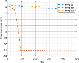
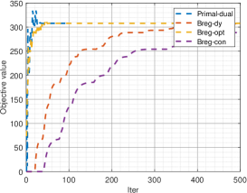
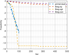
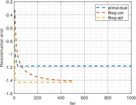
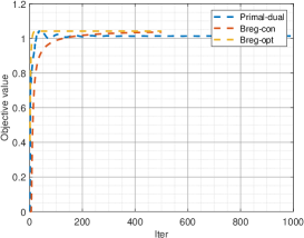
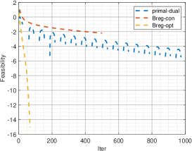
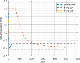
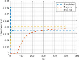
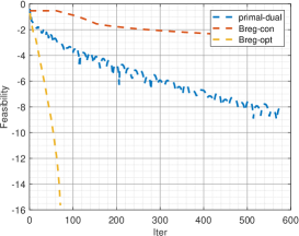
For a given matrix we construct a recoverable sparse vector using L1TestPack [19], compute the corresponding right-hand side , and choose the regularization parameter . The results are summarized in Figure 1. We denote Algorithm 1 with dynamic, exact, and constant step-sizes as “Breg-dy”, “Breg-opt” and “Breg-con”, respectively. The primal-dual method (5.4) is referred to as “primal-dual”. The reconstruction error is defined as , where is the iterate in Algorithm. The objective value denotes . The feasibility is denoted by . Figure 1 (c) shows that All step-sizes have successfully attained feasible solutions, with the exact step size demonstrating linear convergence from the iterative point to the feasible solution, thereby validating Theorem 4.4. Furthermore, all step-sizes have identified the optimal solution for problem (1.2), as illustrated in Figure 1 (b). This is attributed to the fulfillment of the conditions shown in Theorem 4.2 for problem (1.2). Regarding the reconstruction error, it is observed that the exact step size exhibits a smaller reconstruction error compared to other step-sizes.

5.2 Feasibility problems
This subsection considers problem (1.3). In particular, consider the following feasibility problem:
| (5.5) |
where is strongly convex and is an convex set. Denote . Then one can construct an equivalent bilevel optimization problem as follows:
| (5.6) |
The gradient Lipschitz constant of is . Our algorithm has the following iterative scheme:
| (5.7) |
In order to illustrate the performance of Algorithm 1 to solve problem (5.6), we consider the problem of recovering sparse solutions of linear equations , where only noisy data is available for different noise models. In this case, the convex set , where denote the noise. The choice of the norm is dictated by the noise characteristics. In the following, we will consider three types of norms, i.e., the -norm for Gaussian noise and the -norm for uniformly distributed noise. In order to obtain the optimal solution, we also run the primal-dual algorithm to solve (5.6) by letting and .
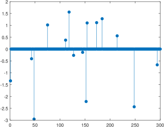
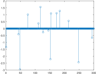
5.2.1 Sparse recovery with Gaussian noise
This subsection focus on an special case of problem (5.6), where , is the noise. In this case
| (5.8) |
For some matrix we produce a sparse vector with only 30 nonzero entries and calculate . We choose by adding the Gaussian noise to , and .
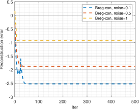
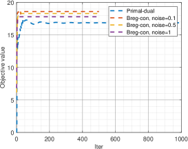
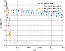
Figure 3 shows the result. Despite the successful identification of feasible solutions for all step-sizes, Figure 3 (b) illustrates that they yield larger objective function values compared to the primal-dual algorithm. This indicates that our algorithm may not necessarily find the optimal solution. The reason lies in the failure of problem (5.6) to satisfy the conditions in Theorem 4.2, thereby indirectly validating the reasonableness of these conditions. Despite the absence of an optimal solution, Figure 3 (a) demonstrates that, under the exact step size, our algorithm accurately recovers the original solution. This further underscores the practical significance of our algorithm. In order to show the effect of the level of noise, we let the noise constant , where . Figure 4 shows that a low level of noise achieves a lower reconstruction error.
5.2.2 Sparse recovery with uniform noise
This subsection focus on an special case of problem (5.6), where , is the noise. In this case
| (5.9) |
For some matrix we produce a sparse vector with only 30 nonzero entries and calculate . We choose by adding uniformly distributed noise with range , and . Figure 5 shows a similar result as the previous subsection. Our algorithm with the exact step-size achieves better performance in terms of the reconstruction error and feasibility.
6 Conclusion
This paper introduces a novel bilevel optimization formulation, offering a cut-and-project perspective to reevaluate Bregman regularized iterations. This approach not only encompasses existing methods but also extends to tackle broader inverse problems, including certain sparse noise models. Through detailed analysis, we explore the impact of step-sizes on algorithmic performance, delineating a practical range for their selection and providing a convergence guarantee to a feasible point. Our unified convergence condition offers a less restrictive criterion compared to existing literature, enhancing the applicability of our framework. Additionally, we introduce a Bregman distance growth condition, proving the linear convergence of our algorithm.
References
- [1] Jean-Bernard Baillon and Georges Haddad. Quelques propriétés des opérateurs angle-bornés et n-cycliquement monotones. Israel Journal of Mathematics, 26:137–150, 1977.
- [2] Heinz H Bauschke, Jonathan M Borwein, et al. Legendre functions and the method of random Bregman projections. Journal of convex analysis, 4(1):27–67, 1997.
- [3] Amir Beck. First-order methods in optimization. SIAM, 2017.
- [4] Amir Beck and Shoham Sabach. A first order method for finding minimal norm-like solutions of convex optimization problems. Mathematical Programming, 147(1-2):25–46, 2014.
- [5] Martin Benning, Marta M Betcke, Matthias J Ehrhardt, and Carola-Bibiane Schönlieb. Choose your path wisely: gradient descent in a Bregman distance framework. SIAM Journal on Imaging Sciences, 14(2):814–843, 2021.
- [6] Lev M Bregman. The relaxation method of finding the common point of convex sets and its application to the solution of problems in convex programming. USSR computational mathematics and mathematical physics, 7(3):200–217, 1967.
- [7] Sébastien Bubeck et al. Convex optimization: Algorithms and complexity. Foundations and Trends® in Machine Learning, 8(3-4):231–357, 2015.
- [8] Jian-Feng Cai, Emmanuel J Candès, and Zuowei Shen. A singular value thresholding algorithm for matrix completion. SIAM Journal on optimization, 20(4):1956–1982, 2010.
- [9] Jian-Feng Cai, Stanley Osher, and Zuowei Shen. Convergence of the linearized Bregman iteration for -norm minimization. Mathematics of Computation, 78(268):2127–2136, 2009.
- [10] Jian-Feng Cai, Stanley Osher, and Zuowei Shen. Linearized Bregman iterations for compressed sensing. Mathematics of computation, 78(267):1515–1536, 2009.
- [11] Jian-Feng Cai, Stanley Osher, and Zuowei Shen. Linearized bregman iterations for frame-based image deblurring. SIAM Journal on Imaging Sciences, 2(1):226–252, 2009.
- [12] Jerome Darbon and Stanley Osher. Fast discrete optimization for sparse approximations and deconvolutions. Preprint, 2007.
- [13] Martin Hanke. Accelerated landweber iterations for the solution of ill-posed equations. Numerische mathematik, 60:341–373, 1991.
- [14] Jean-Baptiste Hiriart-Urruty and Claude Lemaréchal. Fundamentals of convex analysis. Springer Science & Business Media, 2004.
- [15] Stefan Karczmarz. Angenaherte auflosung von systemen linearer glei-chungen. Bull. Int. Acad. Pol. Sic. Let., Cl. Sci. Math. Nat., pages 355–357, 1937.
- [16] Krzysztof C Kiwiel. Free-steering relaxation methods for problems with strictly convex costs and linear constraints. Mathematics of Operations Research, 22(2):326–349, 1997.
- [17] Krzysztof C Kiwiel. Proximal minimization methods with generalized Bregman functions. SIAM journal on control and optimization, 35(4):1142–1168, 1997.
- [18] Ming-Jun Lai and Wotao Yin. Augmented and nuclear-norm models with a globally linearly convergent algorithm. SIAM Journal on Imaging Sciences, 6(2):1059–1091, 2013.
- [19] Dirk A Lorenz. Constructing test instances for basis pursuit denoising. IEEE Transactions on Signal Processing, 61(5):1210–1214, 2012.
- [20] Dirk A Lorenz, Frank Schopfer, and Stephan Wenger. The linearized Bregman method via split feasibility problems: analysis and generalizations. SIAM Journal on Imaging Sciences, 7(2):1237–1262, 2014.
- [21] Haihao Lu, Robert M Freund, and Yurii Nesterov. Relatively smooth convex optimization by first-order methods, and applications. SIAM Journal on Optimization, 28(1):333–354, 2018.
- [22] Ion Necoara, Yu Nesterov, and Francois Glineur. Linear convergence of first order methods for non-strongly convex optimization. Mathematical Programming, 175:69–107, 2019.
- [23] Daniel Reem, Simeon Reich, and Alvaro De Pierro. Re-examination of Bregman functions and new properties of their divergences. Optimization, 68(1):279–348, 2019.
- [24] R Tyrrell Rockafellar. Convex analysis, volume 11. Princeton university press, 1997.
- [25] Frank Schöpfer and Dirk A Lorenz. Linear convergence of the randomized sparse Kaczmarz method. Mathematical Programming, 173:509–536, 2019.
- [26] Wotao Yin. Analysis and generalizations of the linearized Bregman method. SIAM Journal on Imaging Sciences, 3(4):856–877, 2010.
- [27] Wotao Yin, Stanley Osher, Donald Goldfarb, and Jerome Darbon. Bregman iterative algorithms for -minimization with applications to compressed sensing. SIAM Journal on Imaging sciences, 1(1):143–168, 2008.
- [28] Hui Zhang. New analysis of linear convergence of gradient-type methods via unifying error bound conditions. Mathematical Programming, 180(1):371–416, 2020.
- [29] Hui Zhang, Yu-Hong Dai, Lei Guo, and Wei Peng. Proximal-like incremental aggregated gradient method with linear convergence under Bregman distance growth conditions. Mathematics of Operations Research, 46(1):61–81, 2021.
- [30] Hui Zhang, Lu Zhang, and Hao-Xing Yang. Revisiting linearized Bregman iterations under Lipschitz-like convexity condition. Mathematics of Computation, 92(340):779–803, 2023.