Electrical conductivity of QGP with quasiparticle quarks and Gribov gluon

Abstract

We investigate the electrical conductivity of a quark-gluon plasma (QGP) medium using non-perturbative resummation via Gribov gluon propagator. To calculate the electrical conductivity, we utilize the relativistic Boltzmann’s kinetic equation, within the relaxation-time approximation (RTA). The relaxation times are determined by evaluating the microscopic two-body scattering amplitude. We adopt the quasiparticle approach, which allows us to comprehend the transport properties in both the weak and strong coupling regimes. Above the transition temperature, we estimate the electrical conductivity of the quark-gluon plasma using the Gribov prescription and compare our findings with lattice results and various phenomenological models. We find our results in close agreement with the lattice data.

I Introduction

The discovery of quark-gluon plasma (QGP) at the beginning of this century [1, 2] has opened up new possibilities in the field of relativistic heavy-ion collision programs at RHIC and the LHC [3]. One of the key goals of these programs is to extract the precise properties of QGP. Over the past twenty years, researchers have extensively studied the behavior of this matter in both ideal [4, 5, 6, 7, 8] and viscous hydrodynamics [9, 10, 11, 12, 13, 14, 15]. These studies have helped identify the QGP as a strongly-coupled fluid. It is now widely accepted that QGP is a strongly coupled system that behaves like a nearly perfect fluid in heavy-ion collisions. This allows for a hydrodynamic description of QGP, enabling us to gain a better understanding of its behavior and properties [16, 17]. The investigation of various properties of this hot and dense QCD medium (QGP) is an immensely intriguing topic that demands attention. The transport properties characterized by the corresponding transport parameters provide crucial information about the interactions in the medium and are essential theoretical inputs for the hydrodynamic evolution of strongly interacting matter. These parameters are critical tools for analyzing the data from heavy ion collisions  [18, 19, 16].

The electrical conductivity of a hot and dense deconfined nuclear matter has gained attention due to a strong electric field created in the collision zone of ultra-relativistic heavy-ion collision experiments and has been studied by several research groups in various frameworks [20, 21, 22, 23, 24, 25, 26, 27, 28, 29, 30, 31, 32, 33, 34, 35, 36, 37, 38, 39, 40, 41, 42, 43, 44, 45, 46, 47, 48, 49, 50]. In peripheral heavy-ion collisions, a large electrical and magnetic field is generated, which can significantly impact the medium’s behavior [51]. The dynamics of the medium formed during collisions can be significantly affected by a large electrical field. The magnitude of electrical conductivity ($\sigma_{el}$) of the medium plays a crucial role in determining the effect of the electrical field. During the early stage of the collision, the electric currents are generated by the quarks, with $\sigma_{el}$ governing this production process. The value of $\sigma_{el}$ plays a fundamental role in determining the strength of chiral magnetic effect [52], which is a signature of CP violation in strong interactions [53]. In mass asymmetric collisions (such as Cu-Au collisions), the electrical field has a preferred direction, which generates a charge asymmetric flow [32]. The strength of this flow is directly related to $\sigma_{el}$, which is related to the emission rate of soft photons [54, 55].

In this study, we compute the electrical conductivity of the QGP medium using the Gribov-Zwanziger approach. This approach has gained significant attention, particularly after its generalization to finite temperature QCD medium [56, 58]. Studies have shown that the Gribov parameter, $\gamma_{G}$, which is an intrinsic Yang-Mills scale, significantly improves the infrared behavior of QCD and leads to good agreement with lattice results for thermodynamic quantities [58]. Lattice calculations have shown inconsistencies in transport coefficient results, making it necessary to find alternate methods to incorporate non-perturbative features in the theory. We follow the approach suggested by Gribov in his fundamental work [61]. The Gribov dispersion relation provides a simple way to account for the effects of residual confinement on the transport properties of QGP. It was first used in Refs. [63, 64, 65] in the context of kinetic theory and hydrodynamics, where it was applied to a boost-invariant setup. Recently, its impact on observables, such as the dilepton rate and quark number susceptibility, has also been examined [66].

Here, we have followed the recent research on a covariant kinetic theory and transport coefficients for Gribov plasma [67]. The study utilized a quasiparticle-like framework, incorporating a bag correction to pressure and energy density. The temperature dependence of the Gribov parameter and running coupling was determined through matching with lattice results for a system of gluons. These parameters have been used to calculate the electrical conductivity of the QGP medium. Additionally, the shear and bulk viscosity of the QGP medium have been explored using Gribov gluons and quasi-particle quarks [69]. Moreover, the dynamics of heavy quark diffusion coefficients [72, 68], heavy quark complex potential [70], and QCD mesonic screening masses have also been investigated using the Gribov-Zwanziger approach [71].

This article is divided into six sections. Section II discusses the formalism of the current work in detail, where the Gribov parameter ($\gamma_{G}$) and running coupling, $g$ are defined. Section III focuses on the scattering cross-section of the constituent particles and computes the scattering amplitude of quark-quark and quark-antiquark interaction. In Section IV, the relaxation time is revisited, which is based on the weighted thermally averaged quark-quark and quark-antiquark cross-section. Section V investigates the electrical conductivity of the medium by uitilizing the quasiparticle model. Finally, Section VI provides a summary and outlook of the work.

II Formalism

II.1 Gribov parameter ($\gamma_{G}$) and running coupling ($g$)

The Gribov-modified gluon propagator, in the Landu gauge reads [73]

$$\mathcal{D}_{ab}^{\mu\nu}(k)=\delta_{ab}\frac{k^{2}}{k^{4}+\gamma_{G}^{4}}\left(\delta^{\mu\nu}-\frac{k^{\mu}k^{\nu}}{k^{2}}\right)\leavevmode\nobreak\ ,$$ (1)

where $k^{\mu}$ is the gluon four momentum and $\gamma_{G}$ is the Gribov parameter, which is a temperature-dependent function determined by fitting the lattice QCD equation of state [67]. The Gribov parameter was originally introduced by Gribov to explain the non-perturbative confinement region. It’s worth noting that the Gribov parametrization has been extensively studied in the literature to explain deconfined nuclear matter [56, 58, 57, 63, 64, 65, 66, 73]. Reference [58] justifies the use of the Gribov prescription to describe deconfined nuclear matter and explains in detail confinement scenario also works in the deconfined phase.

In this context, $\gamma_{G}$ is determined by formulating the thermodynamics of gluonic plasma using the kinetic theory [67]. To characterize the system’s dynamics, we utilize the energy-momentum tensor, which can be expressed as

$$T_{(0)}^{\mu\nu}=\int dk\cdot k^{\mu}k^{\nu}g^{0}+B_{0}(T)g^{\mu\nu}\leavevmode\nobreak\ .$$ (2)

Here, $B_{0}(T)$ represents the bag pressure, included to ensure thermodynamic consistency in equilibrium. The metric tensor $g^{\mu\nu}$ is considered as $g^{\mu\nu}={\rm diag}(+1,-1,-1,-1)$ and $g^{0}$ signifies the equilibrium distribution function for Gribov plasma, defined as

$$g_{\pm}^{0}=\frac{1}{e^{\epsilon_{\pm}/T}-1},$$ (3)

where $\epsilon_{\pm}=\sqrt{|\textbf{k}|^{2}\pm i\gamma_{G}^{2}}$ with $|\textbf{k}|$ as the three-momentum of the gluons. The Lorentz invariant momentum integral is given by

$$\int dk=\frac{d_{g}}{(2\pi)^{3}}\int d^{3}\textbf{{k}}\int dk_{0}\hskip 2.84544pt2\Theta(k_{0})\hskip 2.84544pt\delta\left(k^{2}+\frac{\gamma_{G}^{4}}{k^{2}}\right)\leavevmode\nobreak\ .$$ (4)

In the above equation, the degeneracy factor, $d_{g}=2\times(N_{c}^{2}-1)=16$. The equilibrium pressure and energy density can be obtained from eq. (2) using the relation

$$\mathcal{P}_{\rm eq}=-\frac{1}{3}\Delta_{\mu\nu}T_{(0)}^{\mu\nu}=\mathcal{P}_{\rm Gribov}-B_{0}(T)\leavevmode\nobreak\ .$$ (5)

$$\mathcal{E}_{\rm eq}=u_{\mu}u_{\nu}T_{(0)}^{\mu\nu}=\mathcal{E}_{\rm Gribov}+B_{0}(T)\leavevmode\nobreak\ .$$ (6)

where $\Delta_{\mu\nu}=g_{\mu\nu}-u_{\mu}u_{\nu}$, $u_{\mu}$ is the fluid four velocities satisfying $u^{\mu}u_{\mu}=1$. In fluid rest frame, $u^{\mu}=(1,0,0,0)=(1,\vec{0})$. $\mathcal{P}_{\rm Gribov}$ and $\mathcal{E}_{\rm Gribov}$ are the particle contribution to pressure and energy density of equilibrium Gribov plasma, which are given by

$$P_{\rm Gribov}=\frac{d_{g}}{(2\pi)^{3}}\int\mathrm{d}^{3}\mathbf{k}\frac{|\mathbf{k}|^{2}}{6}\left(\frac{g^{0}_{+}}{\epsilon_{+}}+\frac{g^{0}_{-}}{\epsilon_{-}}\right),$$ (7)

$$\varepsilon_{\rm Gribov}=\frac{d_{g}}{(2\pi)^{3}}\int\mathrm{d}^{3}\mathbf{k}\frac{1}{2}\left(g^{0}_{+}\epsilon_{+}+g^{0}_{-}\epsilon_{-}\right).$$ (8)

The entropy density of Gribov plasma can be calculated using eqs. (5) and (6) by utilizing the thermodynamic relation

$$s_{\rm Gribov}=\frac{\mathcal{P}_{\rm Gribov}+\mathcal{E}_{\rm Gribov}}{T}=\frac{\mathcal{P}_{eq}+\mathcal{E}_{eq}}{T}=s_{eq}.$$ (9)

To fix the Gribov parameter, $\gamma_{G}$, the first step is to match the temperature dependence of the scaled trace anomaly of lattice results [81], in order to fix the equilibrium thermodynamic quantities. For analytical tractability, the trace anomaly is fitted with a specific functional form [82]

$$\frac{\mathcal{I}_{eq}}{T^{4}}= \frac{\mathcal{I}_{\rm lattice}^{F}}{T^{4}}=\exp\left[-\left(\frac{a_{1}}{\tilde{T}}+\frac{a_{2}}{\tilde{T}^{2}}\right)\right]$$

$$\times\left(\frac{a_{0}}{1+a_{3}{\tilde{T}}^{2}}+\frac{b_{0}({\rm\tanh}[b_{1}\tilde{T}+b_{2}]+1)}{1+c_{1}\tilde{T}+c_{2}\tilde{T}^{2}}\right),$$ (10)

where $\tilde{T}$ is the scaled temperature ($=T/T_{c}$).

$a_{0}$	$a_{1}$	$a_{2}$	$a_{3}$	$b_{0}$	$b_{1}$	$b_{2}$	$c_{1}$	$c_{2}$
$0.23$	$-1.83$	$2.92$	$0.07$	$0.32$	$62.39$	$-62.55$	$-1.98$	$1.08$

Table 1: The parameters extracted from the function (Eq. (10)) after fitting with the lattice data.

For this set of parameters, the scaled pressure can be obtained by

$$\frac{\mathcal{P}_{\rm eq}(T)}{T^{4}}=\frac{\mathcal{P}_{\rm lattice}(T)}{T^{4}}=\frac{\mathcal{P}_{\rm lattice}(T_{eq})}{T_{eq}^{4}}+\int_{T_{eq}}^{T}\frac{d\tilde{T}}{\tilde{T}}\times\frac{\mathcal{I}_{\rm lattice}^{F}}{\tilde{T}^{4}}\leavevmode\nobreak\ ,$$ (11)

where $\mathcal{P}_{\rm lattice}(T_{\rm eq}=0.7\,T_{c})=0.0015$. Following the Eqs. (10) and (11), $\mathcal{I}_{\rm lattice}=\epsilon_{\rm lattice}-3\mathcal{P}_{\rm lattice}$ provides the variation of energy density, $\epsilon$ as a function of scaled temperature. To compute the entropy density, we use the thermodynamic relation, $s_{\rm lattice}=d\mathcal{P}_{\rm lattice}/dT=(\mathcal{P}_{\rm lattice}+\epsilon_{\rm lattice})/T$. Therefore, using Eq. (9) to the entropy density of the Gribov-modified gluon, we can equate, $s_{\rm Gribov}=s_{\rm lattice}$, which yields the fixed values of Gribov parameter, $\gamma_{G}$ as followed in Ref. [67].

The total entropy density of the QGP medium is the sum of the entropy densities of the Gribov-modified gluons and the quasi-particle quarks, i.e

$$s^{\rm QGP}_{\rm total}=s_{\rm Gribov(g)}+s_{\rm qp(q)}\leavevmode\nobreak\ ,$$ (12)

where ’qp(q)’ represents the quasi-particle quark and entropy for qp(q) can be obtained as

$$s_{\rm qp(q)}=\sum_{i=l,\bar{l},s,\bar{s}}\frac{d_{i}}{2\pi^{2}}\int_{0}^{\infty}k^{2}dk\frac{(\frac{4}{3}k^{2}+m_{i}^{2})}{E_{i}T}f_{i}^{0}\leavevmode\nobreak\ .$$ (13)

In Eq. (13), $i\,(=u,\bar{u},d,\bar{d},s,\bar{s})$ is the sum over light and strange (anti-) quarks. $d_{i}$ is the degeneracy factor for spin and color; which reads $d_{q_{l},\bar{q_{l}}}=2\times N_{c}\times N_{q_{l},\bar{q_{l}}}$ for light quarks (anti-quarks), $d_{s,\bar{s}}=2\times N_{c}$ for strange quarks and $d_{g}=2\times(N^{2}_{c}-1)$ for gluons with $N_{c}=3$ and $N_{q_{l}}=2$. Here $f_{i}^{0}$ is the equilibrium distribution for fermions, which is defined as

$$f_{i}^{0}\equiv f_{i}^{0}(E_{i},T)=\frac{1}{e^{E_{i}/T}+1},$$ (14)

where $E_{i}=\sqrt{k^{2}+m^{2}_{i}}$ is the quasi-particles energies in thermal equilibrium with $m_{i}$ as the effective mass. The effective mass depends on the temperature and chemical potential, which arises due to the interaction of quarks and gluons with the surrounding matter and is given by [77]

$$m^{2}_{i}=m^{2}_{i0}+\Pi_{i},$$ (15)

where $m_{i0}$ is bare mass and $\Pi_{i}$ is the dynamically generated self-energy, which can be obtained by using the hard-thermal loop approximation (HTL) in asymptotic forms as

$$\Pi_{q_{l}}(T)=\frac{g^{2}T^{2}}{3}\left(m_{q_{l}0}\sqrt{\frac{6}{gT}}+1\right),$$

$$\Pi_{s}(T)=\frac{g^{2}T^{2}}{3}\left(m_{s0}\sqrt{\frac{6}{gT}}+1\right).$$ (16)

where $m_{q_{l}0}$ and $m_{s0}$ are the bare masses of the light ($u,d$) and strange ($s$) quarks, whose values are taken as $5$ MeV and $95$ MeV respectively. Here we limit our study to the medium at finite temperature and vanishing chemical potential. We are considering the medium which consists of $u$, $d$ and $s$ quarks, which interact via the exchange of Gribov-modified gluons. The interactions of quarks and gluons with the surrounding matter in the medium are encoded in the quasiparticle masses (15), which depends on the running coupling, $g$. Here, we fix the running coupling using the lattice data of entropy density for $(2+1)$ QCD. The fit function for the entropy density for $(2+1)$ QCD ($s_{\rm lattice}^{\rm QGP}$) has been developed like for the gluonic ($N_{f}=0$) case [69]. Therefore, to fix the running coupling, we equated the total entropy density of the QGP medium with the entropy density from lattice as

$$s_{\rm lattice}^{\rm QGP}=s_{\rm{Gribov(g)}}+s_{\rm qp(q)}\leavevmode\nobreak\ .$$ (17)

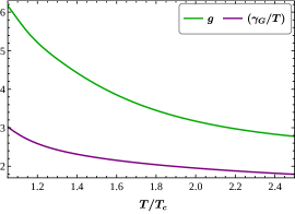
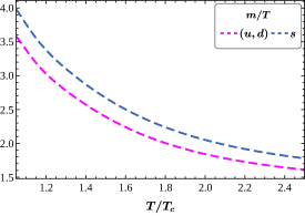
Figure 1: The running coupling $g(T)$ and the scaled Gribov parameter ($\gamma_{G}/T$) as a function of $T/T_{c}$ fitted using the lattice data [83] (upper). The quasiparticle masses (Eq.(16)) for the light (u,d) and strange quarks as a function of scaled temperature (lower).

In the upper plot of figure 1, we show the running coupling, $g(T)$ and scaled Gribov parameter $\gamma_{G}/T$ as a function of scaled temperature ($T/T_{c}$). The data has been fitted using the equation of state of $2+1$ QCD lattice. The critical temperature, $T_{c}$, has been taken as $0.158$ GeV. The green line represents the running coupling and the purple line represents the scaled Gribov parameter. We find that both the Gribov parameter and running coupling decreases monotonically with an increase in temperature above $T_{c}$. In the lower plot, we show the quasiparticle masses for light (pink line ) and strange (blue line) quarks. The quasiparticle masses decreases monotonically with temperature for both light and strange quarks.

III Elastic cross-sections

To analyze the transport properties of QGP medium, it is essential to examine the scattering cross-section of its constituent particles. The differential cross-section for the elastic scattering of the type(1+2 $\rightarrow$ 3+4) is given as

$$\frac{d\sigma}{dt}=\frac{1}{64\pi s}\frac{1}{p_{cm}^{2}}\langle|\bm{\mathcal{M}}|\rangle_{12\rightarrow 34}^{2}\leavevmode\nobreak\ ,$$ (18)

where $p_{cm}$ is the momentum in the center of mass (COM) frame of incoming ($1,2$) and outgoing particles ($3,4$), which can be calculated as

$$p_{cm}=\frac{\sqrt{(s-(m_{1,3}-m_{2,4})^{2})(s-(m_{1,3}+m_{2,4})^{2})}}{2\sqrt{s}}\leavevmode\nobreak\ ,$$ (19)

with $s$ being the Mandelstam variable. Note that in Eq. (18), the invarient matrix amplitude $\langle|\bm{\mathcal{M}}|\rangle_{12\rightarrow 34}^{2}$ is averaged over the initial and summed over the final spin states. These values are computed perturbatively at the tree level for the elementary two-body scattering process involving the massive quasiaprticle quarks/antiquarks and Gribov modified gluons for various possible channels ($s,t,u$), as illustrated in Fig. 2 and Fig. 3. It is worth noting that even though the higher order corrections were not considered in the evaluation of the scattering amplitude, those contributions nevertheless is not necessarily small.

The utilization of different symmetries greatly simplifies the task when assessing the invariant scattering amplitudes involving quark-quark and quark-antiquark interactions. Below are a few examples:

• $\langle|\bm{\mathcal{M}}|^{2}\rangle_{d\bar{d}\rightarrow d\bar{d}}=\langle|\bm{\mathcal{M}}|^{2}\rangle_{u\bar{u}\rightarrow u\bar{u}}$; (charge symmetry).

• $\langle|\bm{\mathcal{M}}|^{2}\rangle_{d\bar{u}\rightarrow d\bar{u}}=\langle|\bm{\mathcal{M}}|^{2}\rangle_{u\bar{d}\rightarrow u\bar{d}}$; (charge conjugation).

• $\langle|\bm{\mathcal{M}}|^{2}\rangle_{u\bar{u}\rightarrow d\bar{d}}(s,t)=\langle|\bm{\mathcal{M}}|^{2}\rangle_{u\bar{d}\rightarrow u\bar{d}}(t,s)$; (crossing symmetry).

• $\langle|\bm{\mathcal{M}}|^{2}\rangle_{uu\rightarrow uu}(u,t)=\langle|\bm{\mathcal{M}}|^{2}\rangle_{u\bar{u}\rightarrow u\bar{u}}(s,t)$; (crossing symmetry).

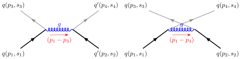
Figure 2: Feynman diagram for $qq^{\prime}\rightarrow qq^{\prime}$ processes. Left: $t-channel$ and Right: $u-channel$, when $q^{\prime}=q$. The black line corresponds to the incoming quarks while the light grey corresponds to the outgoing quarks. The ($p_{i},s_{i}$) is the four-momentum and the spin of the quark so considered.

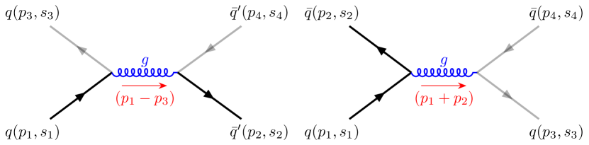
Figure 3: Feynman diagram of $q\bar{q}^{\prime}\rightarrow q\bar{q}^{\prime}$. Left: $t-channel$ and Right: $s-channel$, when $\bar{q}^{\prime}=\bar{q}$. The black line corresponds to the incoming quark/antiquark while the light grey corresponds to the outgoing quark/antiquark. The ($p_{i},s_{i}$) is the four-momentum and the spin of the (anti)quark so considered.

The detailed formulation will be presented elsewhere. However, we note that in the limit $m_{i=1,2,3,4}\rightarrow 0$, our findings of scattering amplitudes are in-line with the one presented in [74]. For the process of $qq(\bar{q})\rightarrow qq(\bar{q})$, the total scattering cross-section ($\sigma_{sc}$) can be expressed as

$$\sigma_{sc}=\int_{t_{-}}^{t_{+}}dt\left(\frac{d\sigma}{dt}\right)[1-f_{3}^{0}(T)][1-f_{4}^{0}(T)]\leavevmode\nobreak\ ,$$ (20)

and for $ug\rightarrow ug$ process can be written as

$$\sigma_{sc}=\int_{t_{-}}^{t_{+}}dt\left(\frac{d\sigma}{dt}\right)[1-f_{3}^{0}(T)][1+g_{4}^{0}(T)]\leavevmode\nobreak\ ,$$ (21)

where $1-f_{3,4}^{0}(T)$ and $1+g_{4}^{0}(T)$ represent the Pauli blocking/Bose enhancement factors for fermions and bosons, respectively. These factors take into account the possibility that some of the final states are already occupied with the constituent particles. The functions $f_{i}^{0}$ and $g_{i}^{0}$ represent the equilibrium distribution functions of the “$i^{th}$” particles of fermions and bosons, respectively, as defined in Eqs. (14) and (3). The integration limit is fixed by considering the collision in the centre of mass frame, where the Mandelstam variable $t=-2p_{cm}^{2}(1-\cos\theta)$ with $-1\leq\cos\theta\leq 1$.

Here all the partonic cross-sections are fixed as a function of temperature ($T$) and Mandelstam variables ($s,t,u$).

III.1 Findings of elastic cross-sections

In this subsection, we present the results of elastic cross-sections for quark-quark, quark-antiquark, and quark-gluon scattering. To provide a comprehensive comparison, we have illustrated each process using plots at two different temperature scales: at $T/T_{c}=1.2$ and $T/T_{c}=2.2$. It is important to note that we calculated the scattering cross-sections for these processes by using the quasiparticle masses of the quarks, as defined in Eq. (16). Moreover, the interaction among the quarks in the QGP medium occurs via gluon exchange, following the Gribov prescription. We used the modified gluon propagator defined in Eq. (1) to account for this interaction.

Here is the list of all possible scattering considered for the $u-$quark, along with their corresponding scattering channels:

1. $u+u\rightarrow u+u;{\hskip 5.69046pt}{\rm\textbf{channel/'s:}}\Rightarrow{\hskip 2.84544pt}t,u$ .

2. $u+d\rightarrow u+d;{\hskip 5.69046pt}{\rm\textbf{channel/'s:}}\Rightarrow{\hskip 2.84544pt}t$ .

3. $u+s\rightarrow u+s;{\hskip 5.69046pt}{\rm\textbf{channel/'s:}}\Rightarrow{\hskip 2.84544pt}t$ .

4. $u+\bar{u}\rightarrow u+\bar{u};{\hskip 5.69046pt}{\rm\textbf{channel/'s:}}\Rightarrow{\hskip 2.84544pt}s,t$ .

5. $u+\bar{u}\rightarrow d+\bar{d};{\hskip 5.69046pt}{\rm\textbf{channel/'s:}}\Rightarrow{\hskip 2.84544pt}s$ .

6. $u+\bar{u}\rightarrow s+\bar{s};{\hskip 5.69046pt}{\rm\textbf{channel/'s:}}\Rightarrow{\hskip 2.84544pt}s$

7. $u+\bar{d}\rightarrow u+\bar{d};{\hskip 5.69046pt}{\rm\textbf{channel/'s:}}\Rightarrow{\hskip 2.84544pt}t$

8. $u+\bar{s}\rightarrow u+\bar{s};{\hskip 5.69046pt}{\rm\textbf{channel/'s:}}\Rightarrow{\hskip 2.84544pt}t$

9. $u+g\rightarrow u+g;{\hskip 5.69046pt}{\rm\textbf{channel/'s:}}\Rightarrow{\hskip 2.84544pt}t$

10. $u+\bar{u}\rightarrow g+g;{\hskip 5.69046pt}{\rm\textbf{channel/'s:}}\Rightarrow{\hskip 2.84544pt}s,t,u$

The same processes apply to both the $d$ and $s$ quarks.

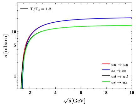
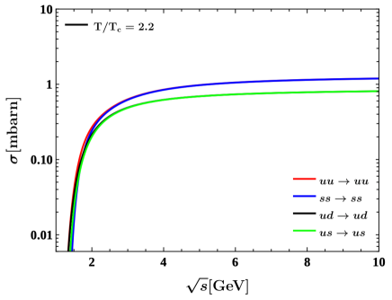
Figure 4: The cross-sections ($\sigma_{sc}$) for the quark-quark scattering are plotted as a function of $\sqrt{s}$, with the left plot corresponding to a scaled temperature of $T/T_{c}=1.2$ and the right plot corresponding to $T/T_{c}=2.2$.

Figure 4 shows the cross-section for quark-quark scattering as a function of $\sqrt{s}$ at two different temperatures, $T/T_{c}=1.2$ (left) and $T/T_{c}=2.2$ (right). Our analysis reveals that the scattering cross-section decreases as a function $\sqrt{s}$ as temperature increases. Specifically, the scattering cross-section experiences a sharp increase at smaller values of $\sqrt{s}$, and then remains constant at higher values of $\sqrt{s}$ above $2.5$ GeV. Interestingly, we observe that the cross-sections are independent of the quasi-masses of the light and strange quarks, and remain the same for both $q+q\rightarrow q+q$ and $q+q^{\prime}\rightarrow q+q^{\prime}$ processes.

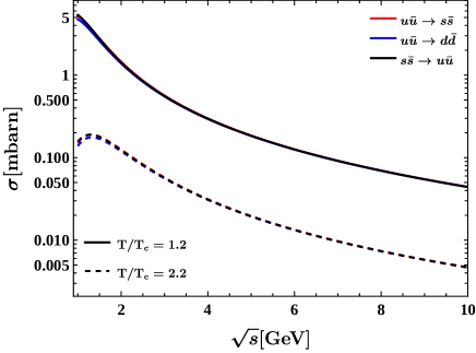
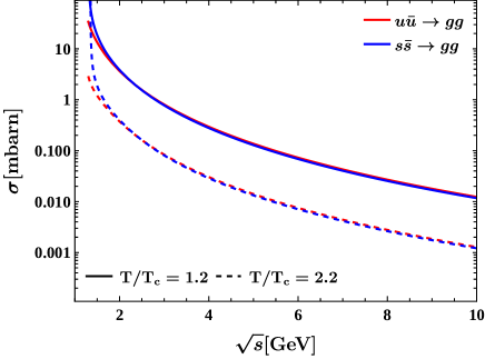
Figure 5: The scattering cross-sections for quark-antiquark (flavour changing) and quark-antiquark pair annihilation as a function of $\sqrt{s}$ at two different scaled temperatures, $T/T_{c}=1.2$ (solid line) and $T/T_{c}=2.2$ (dashed line)

.

Figure 5 demonstrates how the cross-sections vary with the center-of-mass energy ($\sqrt{s}$) for two different processes: flavor-changing quark-antiquark scattering ($q+\overline{q}\rightarrow q^{\prime}+\overline{q}^{\prime}$) on the left, and the pair-annihilation of a quark-antiquark pair ($q+\overline{q}\rightarrow g+g$) on the right. As we can see from the figure, the scattering cross-section for both processes decreases monotonically as $\sqrt{s}$ increases. This behavior is in line with the predictions made by the dynamical quasiparticle model [75]. Interestingly, the difference in quasiparticle mass between light and strange quarks has no significant effect on the scattering cross-sections and remains the same for quark-antiquark scattering. Additionally, the difference in quasiparticle mass between light and strange quarks has minimal impact on the cross-sections of their respective pair-annihilations at smaller values of $\sqrt{s}$. This observation underscores the consistent behavior in the scattering process, regardless of the quark flavors involved.

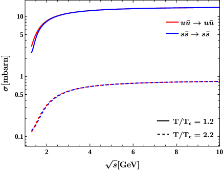
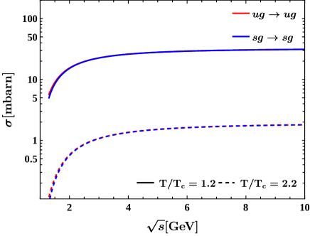
Figure 6: The cross-sections for the quark-antiquark (no flavour change) (left) and quark-gluon (right) scattering as a function $\sqrt{s}$. The solid line corresponds to $T/T_{c}=1.2$ and the dashed line corresponds to $T/T_{c}=2.2$

.

The Fig. 6 illustrates the behavior of the cross-section for quark-antiquark scattering ($q+\overline{q}\rightarrow q+\overline{q}$) (left) and quark-gluon scattering($q+g\rightarrow q+g$) (right) as a function $\sqrt{s}$. Notably, for $\sqrt{s}\geq 3$ GeV, the scattering cross-section remains almost constant for both scaled temperature values, $T/T_{c}=1.2$ (solid line) and $T/T_{c}=2.2$ (dashed line). As the temperature increases, the cross-section value decreases across the entire range of $\sqrt{s}$. This trend demonstrates a significant reduction in the scattering cross-section with increasing temperature. It reflects the impact of temperature variations on the interaction dynamics of quark-antiquark pairs. Note that in evaluating the scattering cross-section of the quark-gluon scattering, we have considered the $t-$channel scattering due to its main contribution.

The next step is to formulate the relaxation time ($\tau_{R}$), which is an essential parameter for calculating the transport coefficients of the QGP medium. This is done using the relaxation time approximation.

IV Relaxation time $(\tau_{R})$

The transport properties of QGP are largely influenced by the relaxation time, $\tau_{R}$, which plays a crucial role in determining various transport coefficients. Therefore, accurately determining this parameter is of paramount importance in understanding the transport properties of QGP. In this study, we have used the method developed in [78] to calculate the relaxation time, $\tau_{R}$, based on the weighted thermally averaged quark-quark and quark-antiquark cross-sections. A similar approach has been previously used in literature to evaluate the relaxation time $\tau_{R}$ [76, 77, 41, 78, 79]. The relaxation time for the species “$i$” is given by

$$\tau_{i}^{-1}(T)=\sum_{i=q,\bar{q}}n_{i}(T)\overline{\sigma}_{12\rightarrow 34}(s,T)\leavevmode\nobreak\ ,$$ (22)

where $\overline{\sigma}_{12\rightarrow 34}$ is the weighted thermal average of the cross-section.

$$\overline{\sigma}_{12\rightarrow 34}=\int_{\rm Th}^{\infty}ds\hskip 2.84544pt\sigma_{12\rightarrow 34}(T,s)\mathcal{X}(T,s)\leavevmode\nobreak\ ,$$ (23)

where the threshold, ${\rm Th=max}\{(m_{1}+m_{2})^{2},(m_{3}+m_{4})^{2}\}$ and $\mathcal{X}(T,s)$ is the probability of finding the quark-quark and quark-antiquark pair with center-of-mass energy $\sqrt{s}$ [80]

$$\mathcal{X}(T,s)=\mathcal{C}\frac{E_{1}^{cm}(\sqrt{s}-E_{1}^{cm})}{\sqrt{s}}p_{cm}f(\sqrt{s}-E_{1}^{cm})f_{0}(E_{1}^{cm})\leavevmode\nobreak\ ,$$ (24)

here $f_{0}(E_{i})$ is the fermionic distribution function for quark-(anti-)quark scattering as defined in eq. ( 14) and $E_{1}^{cm}$ is defined as

$$E_{1}^{cm}(s,T)=\frac{s-(m_{1}(T)^{2}-m_{2}(T)^{2})}{2\sqrt{s}}.$$ (25)

Note that the normalization in the Eq. (24) is fixed by

$$[\mathcal{C}(T)]^{-1}=\int_{\rm Th}^{\infty}ds\hskip 2.84544pt\mathcal{X}(T,s)\leavevmode\nobreak\ .$$ (26)

For the light quarks, the relaxation time is obtained as [76]

$$\tau_{u}^{-1}(T)= n_{\bar{u}}(\overline{\sigma}_{u\bar{u}\rightarrow u\bar{u}}+\overline{\sigma}_{u\bar{u}\rightarrow d\bar{d}}+\overline{\sigma}_{u\bar{u}\rightarrow s\bar{s}}+\overline{\sigma}_{u\bar{d}\rightarrow u\bar{d}}$$

$$+\overline{\sigma}_{u\bar{u}\rightarrow gg})+n_{u}(\overline{\sigma}_{uu\rightarrow uu}+\overline{\sigma}_{ud\rightarrow ud})+n_{s}\overline{\sigma}_{us\rightarrow us}$$

$$+n_{\bar{s}}\overline{\sigma}_{u\bar{s}\rightarrow u\bar{s}}+n_{g}\overline{\sigma}_{ug\rightarrow ug}\leavevmode\nobreak\ ,$$ (27)

and for the strange quark is given as

$$\tau_{s}^{-1}(T)= 2n_{u}\overline{\sigma}_{us\rightarrow us}+2n_{\bar{u}}\overline{\sigma}_{u\bar{s}\rightarrow u\bar{s}}+n_{s}\overline{\sigma}_{ss\rightarrow ss}+$$ (28)

$$n_{\bar{s}}(\overline{\sigma}_{s\bar{s}\rightarrow s\bar{s}}+\overline{\sigma}_{s\bar{s}\rightarrow gg}+2\overline{\sigma}_{s\bar{s}\rightarrow u\bar{u}})+n_{g}\overline{\sigma}_{sg\rightarrow sg}\leavevmode\nobreak\ ,$$

where the degeneracy factor, $d_{i}$, for quarks and gluons is taken as $2\times N_{c}=6$ and $2\times(N_{c}^{2}-1)=16$, respectively. Here $\overline{\sigma}_{12\rightarrow 34}$ is the weighted thermally averaged cross sections, as defined in Eq. (23).

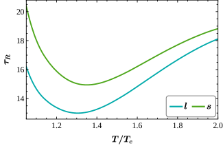
Figure 7: The relaxation time ($\tau_{R}$) as a function of the scaled temperature for the light (Eq. IV) and strange quarks (Eq. 28). The light quark consists of $u$ and $d$ quarks.

In Eq. (IV) and Eq. (28), $n_{i}(T)$ is the equilibrium number density of the particles, which is defined as

$$n_{i}(T)=d_{i}\int\frac{d^{3}p_{i}}{(2\pi)^{3}}f_{i}^{0}\leavevmode\nobreak\ ,$$ (29)

In Figure 7, we present the behavior of relaxation times as a function of scaled temperature. It is measured at vanishing chemical potential. It is observed that the relaxation time for both light and strange quarks first decreases and then increases with temperature.

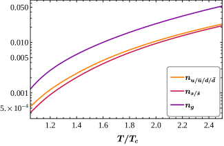
Figure 8: The equilibrium number density of the light and strange quark along with Gribov modified gluons as a function of $T/T_{c}$ in the range $1.05\leq T/T_{c}\leq 2.5$.

In Fig 8, the variation of the number densities of the light quarks and the strange quark is ploted against the scaled temperature $T/T_{c}$. We see that the number density of the Gribov modified gluons peaks the plot for the entire range of scaled temperature.

V Electrical conductivity

In this section, we have compute the electrical conductivity of the QGP medium, which quantifies the ability of a system to conduct the electric charges. After solving the relativistic Boltzmann’s kinetic equation in the relaxation time approximation (RTA), one can obtain the electrical conductivity expression as [40, 84]

$$\sigma_{el}=\frac{1}{3T}\sum_{i}\int\frac{d^{3}k}{(2\pi)^{3}}\frac{k^{2}}{E_{i}^{2}}q_{i}^{2}d_{i}\tau_{i}f_{i}^{0}\left(1-f_{i}^{0}\right),$$ (30)

where $\tau_{i}$ is the relaxation time for quarks (anti-quarks) and gluons respectively, which is defined in section IV. The electric charge $q_{i}$ for u, d and s quarks are $q_{u}=-q_{\bar{u}}=2e/3$ and $q_{d,s}=-q_{\bar{d},\bar{s}}=-e/3$, respectively. The electron charge $e=\sqrt{4\pi\alpha}$ with the fine structure constant, $\alpha=1/137$. $f_{i}^{0}$ is the equilibrium distribution, which is defined in eq. (14).

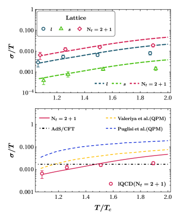
Figure 9: The electrical conductivity as a function of the scaled temperature for different flavors ($l$, $s$, and $N_{f}=2+1$) (upper) and for $N_{f}=2+1$ (lower). The blue, green and red symbol from lattice data [29], blue and yellow lines from QPM [34, 84], and black dot-dashed line from AdS/CFT approach [85].

In Figure 9, we present a plot of the electrical conductivity as a function of scaled temperature. In the upper plot, we compare our electrical conductivity results for different flavors ($l$, $s$, and $N_{f}=2+1$) with the lattice data [29]. The red, blue, and green dashed lines correspond to the light (consisting of $u$ and $d$ quarks), strange, and $N_{f}=2+1$ flavors, respectively, along with the same color symbols taken from the lattice data. In the lower plot, we show the variation of the electrical conductivity for $N_{f}=2+1$ (solid red line) compared with the results from the Quasiparticle Model (QPM) (blue and yellow dashed lines) [34, 84], lattice QCD (red circle), and the black dot-dashed line represents the value of $\sigma/T=e^{2}N_{c}^{2}/16\pi\sim 0.017$ obtained using the AdS/CFT approach [85]. Our results are in close agreement with the lattice data. It is worth noticing that the antiquark contribution to the electrical conductivity($\sigma_{u,d,s}$) has been neglected while comparing our findings with that of the lattice calculation of the same, considering that the lattice findings do not include the contribution from respective antiquarks, and are just for quarks.

VI Summary and outlook

In this work, we have investigated the electrical conductivity scaled with the temperature $T$ for the medium QGP, consisting of light ($u$ and $d$) and strange quarks in the quasiparticle approach, utilizing the kinetic theory framework in relaxation time approximation. The exchanged gluons between the quarks has been modified by the Gribov idea, where the Gribov parameter $\gamma_{G}$ has been fixed using the lattice data of the thermodynamical quantities. Also, the quasi masses of the light and strange quarks is parameterised with the running coupling $g$, which is again fixed making use of the lattice data of the $(2+1)$ QCD.

The relaxation time $\tau_{R}$ has been an important dynamical parameter in determining the transport coefficients, and electrical conductivity is no different. In this project, the relaxation time has been evaluated by thermally averaged cross-section of all the possible quark-(anti)quark scatterings to the lowest order, however, it can be noted that higher order correction may have significant effect on the outcome.

We also investigated the quark flavour dependence of the electrical conductivity and compared it with the available lattice findings of the same. We notice a decent match with the lattice data, specifically near the phase transition temperature. We compared our final result with the previous finding of the electrical conductivity based on quasiparticle model.

References

- [1] M. Gyulassy and L. McLerran, Nucl. Phys. A 750, 30-63 (2005) [arXiv:nucl-th/0405013 [nucl-th]].
- [2] P. Jacobs and X. N. Wang, Prog. Part. Nucl. Phys. 54, 443-534 (2005) [arXiv:hep-ph/0405125 [hep-ph]].
- [3] W. Busza, K. Rajagopal and W. van der Schee, Ann. Rev. Nucl. Part. Sci. 68, 339-376 (2018) [arXiv:1802.04801 [hep-ph]].
- [4] D. Teaney, J. Lauret and E. V. Shuryak, Phys. Rev. Lett. 86, 4783-4786 (2001) [arXiv:nucl-th/0011058 [nucl-th]].
- [5] P. Huovinen, P. F. Kolb, U. W. Heinz, P. V. Ruuskanen and S. A. Voloshin, Phys. Lett. B 503, 58-64 (2001) [arXiv:hep-ph/0101136 [hep-ph]].
- [6] T. Hirano and K. Tsuda, Phys. Rev. C 66, 054905 (2002) [arXiv:nucl-th/0205043 [nucl-th]].
- [7] W. Broniowski, M. Chojnacki, W. Florkowski and A. Kisiel, Phys. Rev. Lett. 101, 022301 (2008) [arXiv:0801.4361 [nucl-th]].
- [8] B. Schenke, S. Jeon and C. Gale, Phys. Rev. C 82, 014903 (2010) [arXiv:1004.1408 [hep-ph]].
- [9] P. Romatschke and U. Romatschke, Phys. Rev. Lett. 99, 172301 (2007) [arXiv:0706.1522 [nucl-th]].
- [10] H. Song and U. W. Heinz, Phys. Lett. B 658, 279-283 (2008) [arXiv:0709.0742 [nucl-th]], J. Phys. G 36, 064033 (2009) [arXiv:0812.4274 [nucl-th]], Phys. Rev. C 81, 024905 (2010) [arXiv:0909.1549 [nucl-th]].
- [11] K. Dusling and D. Teaney, Phys. Rev. C 77, 034905 (2008) [arXiv:0710.5932 [nucl-th]].
- [12] P. Bozek, Phys. Rev. C 81, 034909 (2010) [arXiv:0911.2397 [nucl-th]].
- [13] P. Bozek and I. Wyskiel-Piekarska, Phys. Rev. C 85, 064915 (2012) [arXiv:1203.6513 [nucl-th]].
- [14] S. Ryu, J. F. Paquet, C. Shen, G. S. Denicol, B. Schenke, S. Jeon and C. Gale, Phys. Rev. Lett. 115, no.13, 132301 (2015) [arXiv:1502.01675 [nucl-th]], Phys. Rev. C 97, no.3, 034910 (2018) [arXiv:1704.04216 [nucl-th]].
- [15] L. Du and U. Heinz, Comput. Phys. Commun. 251, 107090 (2020) [arXiv:1906.11181 [nucl-th]].
- [16] U. Heinz and R. Snellings, Ann. Rev. Nucl. Part. Sci. 63, 123-151 (2013) [arXiv:1301.2826 [nucl-th]].
- [17] S. Jeon and U. Heinz, Int. J. Mod. Phys. E 24, no.10, 1530010 (2015) [arXiv:1503.03931 [hep-ph]].
- [18] C. Gale, S. Jeon and B. Schenke, Int. J. Mod. Phys. A 28, 1340011 (2013) [arXiv:1301.5893 [nucl-th]].
- [19] B. Schenke, S. Jeon and C. Gale, J. Phys. G 38, 124169 (2011).
- [20] P. B. Arnold, G. D. Moore and L. G. Yaffe, JHEP 0011, 001 (2000).
- [21] P. B. Arnold, G. D. Moore and L. G. Yaffe, JHEP 0305, 051 (2003).
- [22] S. Gupta,Phys. Lett. B 597 , 57 (2004).
- [23] G. Aarts, C. Allton, J. Foley, S. Hands and S. Kim, Phys. Rev. Lett. 99, 022002 (2007)
- [24] P. V. Buividovich, M. N. Chernodub, D. E. Kharzeev, T. Kalaydzhyan, E. V. Luschevskaya and M. I. Polikarpov, Phys. Rev. Lett. 105, 132001 (2010).
- [25] H.-T. Ding, A. Francis, O. Kaczmarek, F. Karsch, E. Laermann and W. Soeldner, Phys. Rev. D 83, 034504 (2011).
- [26] Y. Burnier and M. Laine, Eur. Phys. J. C 72, 1902 (2012).
- [27] B. B. Brandt, A. Francis, H. B. Meyer and H. Wittig, JHEP 1303, 100 (2013).
- [28] A. Amato, G. Aarts, C. Allton, P. Giudice, S. Hands and J. I. Skullerud, Phys. Rev. Lett. 111, no. 17, 172001 (2013).
- [29] G. Aarts, C. Allton, A. Amato, P. Giudice, S. Hands and J. I. Skullerud, JHEP 1502, 186 (2015).
- [30] W. Cassing, O. Linnyk, T. Steinert and V. Ozvenchuk, Phys. Rev. Lett. 110, no. 18, 182301 (2013).
- [31] T. Steinert and W. Cassing, Phys. Rev. C 89, no. 3, 035203 (2014).
- [32] Y. Hirono, M. Hongo and T. Hirano, Phys. Rev. C 90, no. 2, 021903 (2014).
- [33] M. Greif, I. Bouras, C. Greiner and Z. Xu, Phys. Rev. D 90, no. 9, 094014 (2014).
- [34] A. Puglisi, S. Plumari and V. Greco, Phys. Lett. B 751, 326 (2015).
- [35] A. Puglisi, S. Plumari and V. Greco, Phys. Rev. D 90, 114009 (2014).
- [36] S. I. Finazzo and J. Noronha, Phys. Rev. D 89, no. 10, 106008 (2014).
- [37] M. Greif, C. Greiner and G. S. Denicol, Phys. Rev. D 93, no. 9, 096012 (2016).
- [38] S. Mitra and V. Chandra, Phys. Rev. D 94, no. 3, 034025 (2016).
- [39] P. K. Srivastava, L. Thakur and B. K. Patra, Phys. Rev. C 91, no. 4, 044903 (2015).
- [40] L. Thakur, P. K. Srivastava, G. P. Kadam, M. George and H. Mishra, Phys. Rev. D 95, 096009 (2017).
- [41] R. Marty, E. Bratkovskaya, W. Cassing, J. Aichelin and H. Berrehrah, Phys. Rev. C 88, 045204 (2013).
- [42] D. Fernández-Fraile and A. Gomez Nicola, Phys. Rev. D 73, 045025 (2006).
- [43] G. P. Kadam, H. Mishra and L. Thakur, Phys. Rev. D 98, no. 11, 114001 (2018).
- [44] L. Thakur and P. K. Srivastava, Phys. Rev. D 100, no.7, 076016 (2019) [arXiv:1910.12087 [hep-ph]].
- [45] H. Berrehrah, E. Bratkovskaya, T. Steinert and W. Cassing, Int. J. Mod. Phys. E 25, no.07, 1642003 (2016) [arXiv:1605.02371 [hep-ph]].
- [46] S. Mitra and V. Chandra, Phys. Rev. D 97, no.3, 034032 (2018) [arXiv:1801.01700 [nucl-th]].
- [47] O. Soloveva, P. Moreau and E. Bratkovskaya, Phys. Rev. C 101, no.4, 045203 (2020) [arXiv:1911.08547 [nucl-th]].
- [48] P. Singha, A. Abhishek, G. Kadam, S. Ghosh and H. Mishra, J. Phys. G 46, no.1, 015201 (2019) [arXiv:1705.03084 [nucl-th]].
- [49] S. Mitra and V. Chandra, Phys. Rev. D 96, no.9, 094003 (2017) [arXiv:1702.05728 [nucl-th]].
- [50] R. Ghosh and I. A. Shovkovy, [arXiv:2404.01388 [hep-ph]].
- [51] K. Tuchin, Adv. High Energy Phys. 2013, 490495 (2013).
- [52] K. Fukushima, D. E. Kharzeev and H. J. Warringa, Phys. Rev. D 78, 074033 (2008).
- [53] D. E. Kharzeev, L. D. McLerran and H. J. Warringa, Nucl. Phys. A 803, 227 (2008).
- [54] S. Turbide, R. Rapp and C. Gale, Phys. Rev. C 69, 014903 (2004) [arXiv:hep-ph/0308085 [hep-ph]].
- [55] O. Linnyk, W. Cassing and E. L. Bratkovskaya, Phys. Rev. C 89, no.3, 034908 (2014) [arXiv:1311.0279 [nucl-th]].
- [56] D. Zwanziger, Phys. Rev. Lett. 94, 182301 (2005) [arXiv:hep-ph/0407103 [hep-ph]].
- [57] K. Fukushima and N. Su, Phys. Rev. D 88, 076008 (2013)[arXiv:1304.8004 [hep-ph]].
- [58] D. Zwanziger, Phys. Rev. D 76, 125014 (2007) [arXiv:hep-ph/0610021 [hep-ph]].
- [59] N. Su and K. Tywoniuk, Phys. Rev. Lett. 114, no.16, 161601 (2015) doi:10.1103/PhysRevLett.114.161601 [arXiv:1409.3203 [hep-ph]].
- [60] H. B. Meyer, Phys. Rev. Lett. 100, 162001 (2008) [arXiv:0710.3717 [hep-lat]], Phys. Rev. D 76, 101701 (2007) [arXiv:0704.1801 [hep-lat]].
- [61] V. N. Gribov, Nucl. Phys. B 139, 1 (1978).
- [62] D. Zwanziger, Nucl. Phys. B 323, 513-544 (1989).
- [63] W. Florkowski, R. Ryblewski, N. Su and K. Tywoniuk, Phys. Rev. C 94, no.4, 044904 (2016) [arXiv:1509.01242 [hep-ph]].
- [64] W. Florkowski, R. Ryblewski, N. Su and K. Tywoniuk, Acta Phys. Polon. B 47, 1833 (2016) [arXiv:1504.03176 [hep-ph]].
- [65] V. Begun, W. Florkowski and R. Ryblewski, Acta Phys. Polon. B 48, 125 (2017) [arXiv:1602.08308 [nucl-th]].
- [66] A. Bandyopadhyay, N. Haque, M. G. Mustafa and M. Strickland, Phys. Rev. D 93, no.6, 065004 (2016) [arXiv:1508.06249 [hep-ph]].
- [67] A. Jaiswal and N. Haque, Phys. Lett. B 811, 135936 (2020) [arXiv:2005.01303 [hep-ph]].
- [68] Sumit, A. Mukherjee, N. Haque and B. K. Patra, [arXiv:2311.18560 [hep-ph]].
- [69] S. Madni, A. Mukherjee, A. Jaiswal and N. Haque, [arXiv:2401.08384 [hep-ph]].
- [70] M. Debnath, R. Ghosh and N. Haque, [arXiv:2305.16250 [hep-ph]].
- [71] Sumit, N. Haque and B. K. Patra, Phys. Lett. B 845, 138143 (2023) [arXiv:2305.08525 [hep-ph]].
- [72] S. Madni, A. Mukherjee, A. Bandyopadhyay and N. Haque, Phys. Lett. B 838, 137714 (2023) [arXiv:2210.03076 [hep-ph]].
- [73] N. Su and K. Tywoniuk, Phys. Rev. Lett. 114, no.16, 161601 (2015) doi:10.1103/PhysRevLett.114.161601 [arXiv:1409.3203 [hep-ph]].
- [74] R. Cutler and D. W. Sivers, Phys. Rev. D 17, 196 (1978) doi:10.1103/PhysRevD.17.196
- [75] P. Moreau, O. Soloveva, L. Oliva, T. Song, W. Cassing and E. Bratkovskaya, Phys. Rev. C 100, no.1, 014911 (2019) doi:10.1103/PhysRevC.100.014911 [arXiv:1903.10257 [nucl-th]].
- [76] O. Soloveva, D. Fuseau, J. Aichelin and E. Bratkovskaya, Phys. Rev. C 103, no.5, 054901 (2021) doi:10.1103/PhysRevC.103.054901 [arXiv:2011.03505 [nucl-th]].
- [77] V. Mykhaylova, M. Bluhm, K. Redlich and C. Sasaki, Phys. Rev. D 100, no.3, 034002 (2019) doi:10.1103/PhysRevD.100.034002 [arXiv:1906.01697 [hep-ph]].
- [78] C. Sasaki and K. Redlich, Nucl. Phys. A 832, 62-75 (2010) doi:10.1016/j.nuclphysa.2009.11.005 [arXiv:0811.4708 [hep-ph]].
- [79] P. Danielewicz and M. Gyulassy, Phys. Rev. D 31, 53-62 (1985) doi:10.1103/PhysRevD.31.53
- [80] H. Berrehrah, E. Bratkovskaya, W. Cassing, P. B. Gossiaux, J. Aichelin and M. Bleicher, Phys. Rev. C 89, no.5, 054901 (2014) doi:10.1103/PhysRevC.89.054901 [arXiv:1308.5148 [hep-ph]].
- [81] S. Borsanyi, G. Endrodi, Z. Fodor, S. D. Katz and K. K. Szabo, JHEP 07, 056 (2012) [arXiv:1204.6184 [hep-lat]].
- [82] S. Borsanyi, G. Endrodi, Z. Fodor, A. Jakovac, S. D. Katz, S. Krieg, C. Ratti and K. K. Szabo, JHEP 11, 077 (2010) [arXiv:1007.2580 [hep-lat]].
- [83] S. Borsanyi, Z. Fodor, C. Hoelbling, S. D. Katz, S. Krieg and K. K. Szabo, Phys. Lett. B 730, 99-104 (2014) doi:10.1016/j.physletb.2014.01.007 [arXiv:1309.5258 [hep-lat]].
- [84] V. Mykhaylova and C. Sasaki, Phys. Rev. D 103, no.1, 014007 (2021) [arXiv:2007.06846 [hep-ph]].
- [85] S. Caron-Huot, P. Kovtun, G. D. Moore, A. Starinets and L. G. Yaffe, JHEP 12, 015 (2006) doi:10.1088/1126-6708/2006/12/015 [arXiv:hep-th/0607237 [hep-th]].