Effective Reinforcement Learning Based on Structural Information Principles

Abstract

Although Reinforcement Learning (RL) algorithms acquire sequential behavioral patterns through interactions with the environment, their effectiveness in noisy and high-dimensional scenarios typically relies on specific structural priors. In this paper, we propose a novel and general Structural Information principles-based framework for effective Decision-Making, namely SIDM, approached from an information-theoretic perspective. This paper presents a specific unsupervised partitioning method that forms vertex communities in the state and action spaces based on their feature similarities. An aggregation function, which utilizes structural entropy as the vertex weight, is devised within each community to obtain its embedding, thereby facilitating hierarchical state and action abstractions. By extracting abstract elements from historical trajectories, a directed, weighted, homogeneous transition graph is constructed. The minimization of this graph’s high-dimensional entropy leads to the generation of an optimal encoding tree. An innovative two-layer skill-based learning mechanism is introduced to compute the common path entropy of each state transition as its identified probability, thereby obviating the requirement for expert knowledge. Moreover, SIDM can be flexibly incorporated into various single-agent and multi-agent RL algorithms, enhancing their performance. Finally, extensive evaluations on challenging benchmarks demonstrate that, compared with SOTA baselines, our framework significantly and consistently improves the policy’s quality, stability, and efficiency up to $32.70\%$, $88.26\%$, and $64.86\%$, respectively.

[1]organization=State Key Laboratory of Software Development Environment, School of Computer Science and Engineering, Beihang University,city=Beijing, postcode=100191, country=China

[2]organization=School of Cyber Science and Technology, Beihang University,city=Beijing, postcode=100191, country=China

1 Introduction

Reinforcement Learning (RL) [32] is a promising method for addressing goal-directed sequential decision-making problems, where agents learn the optimal action in each state through interactions with the environment. The integration of deep learning advancements [33, 34] with RL has given rise to Deep Reinforcement Learning (DRL) [35, 36]. This new field utilizes powerful function approximators and has demonstrated promising results in various tasks including Game Intelligence [77, 37, 81], Video Acceleration [111], and Robust Model Fitting [110]. However, in environments with noisy and high-dimensional observations, DRL frequently requires extensive experience gathering to formulate a decision-making policy, a process that is often ineffective, unstable, and sample-inefficient [38]

State abstraction disregards irrelevant environmental details and condenses the state space to considerably streamline the original decision-making process [45, 63]. Prior abstraction research has focused on defining aggregation functions that cluster analogous states, thereby diminishing task complexity [46, 47]. However, their performances rely heavily on specific aggregation parameters, such as the predicate constant in approximate abstraction and the bucket size in transitive abstraction. In contrast, recent studies have explored various representation-learning objectives to attain more desirable state representations [68, 69]. While these representations possess strong capacities, they discard essential environmental information, resulting in inaccurate characterizations of the original decision process. Consequently, achieving a balance between eliminating irrelevant details and preserving essential information is crucial for effective decision-making [52]. Markov state abstraction [51], is employed to achieve the aforementioned balance, ensuring sufficient representational capacity while accurately capturing the original rewards and transition dynamics. However, an unavoidable loss of critical information occurs due to random sampling from finite replay buffers, affecting its performance on challenging tasks.

Skill-based learning [70, 71] represents an alternative mechanism to enhance the sample efficiency of single-agent RL algorithms. This mechanism functions on a dual-level: the lower level acquires skills for diverse sub-problems, which the higher level selects the optimal skill to accomplish task goal. However, most existing research [73, 72] makes explicit or implicit assumptions about pre-defined task structures or skill models. The requirement for prior knowledge entails a trade-off between sample efficiency and policy generality. To address this, the HSD-3 algorithm is introduced to pre-train a skill hierarchy that provides both task generality and sufficient exploration capabilities [75]. But its unsupervised pre-training phase still depends on manual feature selection and transformation. Reskill [113] employs generative models to sample relevant skills, thus facilitating accelerated exploration. As skills in this model are delineated as original observation and action sequences, its performance is contingent upon the representing and sampling methods for environmental interactions. Hence, developing an adaptive and stable skill-based learning mechanism that functions independently of prior knowledge remains a critical challenge in this domain.

In Multi-Agent Reinforcement Learning (MARL) scenarios, the strategy of decomposing decision-making tasks by integrating agent roles is a viable approach to addressing scalability and efficiency challenges [98, 101]. Within this paradigm, each role is distinguished by a specific subtask and an associated role policy that operates within a defined action subspace [2]. Decomposing the cooperative task hinges on the successful identification and integration of a comprehensive set of roles. Typical methods of predefining task decomposition or role assignment [99, 2] require unavailable prior knowledge about subtask-specific rewards or role responsibilities in practice. Moreover, automatically learning an appropriate set of roles from scratch [100, 85] is impractical because it demands substantial explorations in the joint state-action space. Instead, RODE [86] introduces an action abstraction method, employing clustering techniques in the joint action space, to facilitate the discovery of roles. However, its performance largely depends on manual experience and the parameters of adopted clustering algorithms, such as the cluster number of K-means, the maximum and minimum cluster number of X-means, and the neighborhood radius and density threshold of DBSCAN . Absent manual intervention, current role-based methods [85, 86] struggle to guarantee successful role discovery, often due to the absence of clear definitions or the dynamism inherent in practical task decompositions.

To address above challenges, we propose a novel and general Decision-Making framework grounded in Structural Information principles, namely SIDM, with stable effectiveness under complex environments. Initially, we measure feature similarities of states and actions to construct two homogeneous, weighted, undirected graphs: a state graph and an action graph. In each graph, we quantify the uncertainty inherent in random walks between vertices as structural entropy and minimize this uncertainty, partitioning similar states or actions into a single community. To ignore irrelevant noise and preserve essential information, we then design an aggregation function that incorporates assigned entropy as vertex weights within each community. This leads to hierarchical abstractions of states and actions, transforming from noisy individual features to community embeddings, termed as ‘abstract states’ or ‘abstract actions’. Subsequently, we extract abstract elements from historical trajectories to form a directed, weighted, homogeneous graph, encapsulating the multi-relational environmental transitions. By defining and optimizing structural entropy specifically for directed graphs, we generate an optimal encoding tree for this transition graph. For each original transition, we trace the common path of abstract state nodes and calculate the transition’s identified probability based on the cumulative entropy along this path, which is crucial for skill identification. Therefore, we introduce an innovative two-layer learning mechanism, which operates independently of expert knowledge and is tailored for skill-based RL settings. Furthermore, our proposed SIDM is a general framework flexibly integrated with various single-agent and multi-agent RL algorithms for performance improvements.

Our preliminary work was accepted in the proceedings of the AAAI Conference [31] and IJCAI Conference [30]. This journal version expands upon our initial work, integrating the SR-MARL action abstraction and SISA state abstraction into a unified and general framework suitable for both single-agent and multi-agent contexts. This enhanced version features notable enhancements in both methodology and structure of our proposed frameworks. Building on our prior work with similarity graphs, we further transform heterogeneous environmental transitions, driven by multiple actions, into homogeneous transitions between abstract states through abstract actions, effectively preventing the loss of critical information inherent in the original process. To overcome constraints of undirected graphs, we have defined and optimized high-dimensional structural entropy for directed graphs. By calculating entropy along common paths, we determine the sampled probability of each abstract transition and introduce an adaptive two-layer skill-based learning mechanism, thereby enriching the framework’s structure.

In the experimental section, we undertake more comprehensive experiments and analyses across diverse benchmarks, encompasssing visual gridworld navigation, continuous DMControl tasks, robotic control challenge (bipedal robot and 7-Dof arm), and StarCraft II micro-management, with more advanced baselines highlighting our framework’s advantages. Comparative results demonstrate that, SIDM significantly improves the quality of final policies over state-of-the-art algorithms by up to $32.70\%$ and $5.19\%$ in single- and multi-agent scenarios, respectively. Additionally, the SIDM framework boosts sample efficiency by $64.86\%$ and achieves an $88.26\%$ improvement in stability. We also perform a series of ablation studies in above tasks to showcase the generality of SIDM and the importance of different functional modules. The source code and demonstration videos for our SIDM are publicly available on GitHub.

The main contributions of this paper are as follows:

$\bullet$ A novel and general structural information principles-based decision-making framework SIDM is proposed, which can be flexibly integrated with various single- and multi-agent RL algorithms to improve their performances.

$\bullet$ Within each community, an aggregation function is designed that utilizes assigned entropy as the vertex weight, tailored for hierarchical state and action abstractions.

$\bullet$ Leveraging the hierarchical abstractions, a directed and homogeneous graph representing multi-relational environmental transition is constructed to preserve critical information inherent in the original process.

$\bullet$ An adaptive two-layer skill-based learning mechanism independent of expert knowledge is introduced to calculate each state transition’s sampled probability using common path entropy in encoding tree.

$\bullet$ Extensive and empirical experiments are conducted to demonstrate that, compared with the existing SOTA RL algorithms, the proposed SIDM significantly improves the policy’s quality, stability, and sample efficiency under single- and multi-agent decision-making scenarios.

This paper is organized as follows: Section 2 outlines the preliminaries and notation descriptions, Section 3 describes the SIDM’s detailed designs, Sections 4 and 5 discuss the experimental setups and evaluations, and Section 6 introduces the related work before our conclusion in Section 7.

2 Preliminaries and Notations

In this section, we provide a summary of the primary notations outlined in Table 1 and formalize the definitions of several fundamental concepts: the Markov Decision Process (MDP), State or Action Abstraction, Skill-based Learning, Decentralized Partially Observable MDP (Dec-POMDP), Role-based Learning, Homogeneous Weighted Undirected and Directed Graphs, Encoding Tree, and Structural Entropy. In our study, we make a clear distinction between the terms ”observations and original actions” and ”states and actions” to explicitly denote the environmental variables and their respective embedded variables.

Table 1: Glossary of Notations.

Notation	Description
$\mathcal{M}_{s};\mathcal{M}_{m};\mathcal{M}_{\phi}$	Single-agent, Multi-agent, and Abstract Markov decision processes
$n_{i};\mathcal{N}$	Single agent; Agent set
$\mathcal{O};\mathcal{S};\mathcal{A}$	Observation, state, and action spaces
$O;S;A$	Observation, state, and action variables
$o;s;a$	Single observation; Single state; Single action
$z;Z;\mathcal{Z}$	Abstract element; Abstract variable; Abstract space
$r;\mathcal{R};\mathcal{R}_{\phi}$	Reward; Reward function; Abstract reward function
$\mathcal{P};\mathcal{P}_{\phi}$	Transition function; Abstract transition function
$\rho;\Psi;t_{i}$	Role; Role set; Subtask
$\pi;\pi_{\rho};\gamma$	Agent policy; Role policy; Discount factor
$\mathcal{Q};\Omega;f$	Q-value function; Observation function; Embedding function
$\tau;\mathcal{T}$	Individual action-observation history; Action-observation history set
$G;G_{dir}$	Homogeneous weighted undirected and directed graphs
$G_{s};G_{a};G^{*}$	State graph; Action graph; Sparse graph
$v;d_{v};V$	Vertex; Vertex degree; Vertex set
$e;E;E_{dir}$	Edge; Set of undirected edges; Set of directed edges
$w;W;W_{dir}$	Edge weight; Weight functions for undirected and directed edges
$m;n$	Vertex number; Edge number
$\lambda;\alpha;\nu;T$	Root node; Tree node; Leaf node; Encoding tree
$V_{\alpha};\mathcal{V}$	Vertex subset; Volume
$H;M$	Structural entropy; Modification factor
$L;K$	Number of children node; Maximal height of encoding tree
$\eta_{s};\eta_{c};U_{i}$	Stretch operator; Compress operator; Node layer
$\mathcal{K}$	Skill set
$f;h_{s};\mathcal{C}$	Encoder model; Embedded representation; State or action correlation
$\theta;\mathcal{L}$	Training parameter; Training loss
$c;p$	Cluster center; Assignment probability
$P;Q$	Soft and high-confidence assignment matrices
$\text{k};k$	Parameter; Vertex index

Definition 1.

In RL, the single-agent decision-making problem is modeled as a MDP [57], defined by the tuple $\mathcal{M}_{s}=(\mathcal{S},\mathcal{A},\mathcal{R},\mathcal{P},\gamma)$. Here, $\mathcal{S}$ is the original state space, $\mathcal{A}$ is the original action space, $\mathcal{R}$ is the reward function, $\mathcal{P}$ is the transition function, and $\gamma\in[0,1)$ is the discount factor. At each timestep $t$, the agent embeds the environmental observation $o_{t}$ as a state $s_{t}\in\mathcal{S}$ and selects an action $a_{t}\in\mathcal{A}$ according to its policy function $a_{t}\sim\pi(s_{t})$. This action yields a reward $r_{t}\sim\mathcal{R}(s_{t},a_{t})\in\mathbb{R}$ and leads to a new environmental observation $o_{t+1}\sim\mathcal{P}(o_{t},a_{t})$. The objective of RL agent is to learn a policy $\pi$ that maximizes the long-term expected discounted reward, formulated as: $\max_{\pi}\mathbb{E}_{\mathcal{P}}\left[\sum_{t=0}^{\infty}\left[\gamma^{t}\mathcal{R}\left(s_{t},a_{t}\right)\right]\right]$.

Definition 2.

The goal of state or action abstraction is to develop an abstract function $f_{\phi}$ that projects each original state $s\in\mathcal{S}$ or action $a\in\mathcal{A}$ to an abstract element $z_{s}\in\mathcal{Z}_{s}$ or $z_{a}\in\mathcal{Z}_{a}$. This projection is instrumental for the effective reduction of the state-action space, resulting in an abstract MDP $\mathcal{M}_{\phi}=\left(\mathcal{Z}_{s},\mathcal{Z}_{a},\mathcal{R}_{\phi},\mathcal{P}_{\phi},\gamma\right)$.

Definition 3.

In skill-based learning, the agent selects different skills during an episode, with each skill characterized as an original state-action sequence. A skill set $\mathcal{K}$, when applied over a MDP, induces a hierarchical policy structure, where the high-level policy select a skill and the low-level policy outputs atomic actions conditioned on the specific skill. The calculation of long-term expected reward encompasses policies at all hierarchical levels.

Definition 4.

In a partially observable setting, a fully cooperative multi-agent decision-making task is modeled as a Dec-POMDP [87], represented by $\mathcal{M}_{m}=\langle\mathcal{N},\mathcal{S},\mathcal{A},\mathcal{P},\Omega,\mathcal{R},\gamma\rangle$. Here, $\mathcal{N}\equiv\{n_{1},n_{2},\ldots,n_{|\mathcal{N}|}\}$ is the finite set of agents, $\mathcal{S}$ is the global state space, $\mathcal{A}$ is the global action space, $\mathcal{P}$ is the global transition function, $\Omega$ is the observation probability function, $\mathcal{R}$ is the joint reward function, and $\gamma\in[0,1)$ is the discount factor. At each time step, each agent $n_{i}\in\mathcal{N}$ receives a partial observation $o_{i}$ according to the function $\Omega$, and selects an action $a_{i}\in\mathcal{A}$ based on the global state $s\in\mathcal{S}$. These individual actions form a joint action $\bm{a}\equiv\left[a_{i}\right]_{i=1}^{|\mathcal{N}|}$. Subsequently, $\bm{a}$ results in a joint reward $r=\mathcal{R}(s,\bm{a})$ and a transition to the next global state $s^{\prime}\sim\mathcal{P}(\cdot\mid s,\bm{a})$. Each agent $n_{i}$ maintains an action-observation history $\tau_{i}\in\mathcal{T}$ and trains its policy $\pi_{i}\left(a_{i}\mid\tau_{i}\right)$ to maximize the team performance.

Definition 5.

In role-based learning [100, 86], a multi-agent cooperative task $\mathcal{M}_{m}$ is decomposed into a subtask set, where the role set $\Psi$ specifies this decomposition. Each role $\rho_{j}\in\Psi$ is a tuple $\left\langle t_{j},\pi_{\rho_{j}}\right\rangle$, where $t_{j}$ is a subtask defined as $\langle\mathcal{N}_{j},\mathcal{S},\mathcal{A}_{j},\mathcal{P},\Omega,\mathcal{R},\gamma\rangle$ and $\pi_{\rho_{j}}:\tau\times A_{j}\mapsto[0,1]$ is a role policy for $t_{j}$. In the subtask $t_{j}$, $\mathcal{N}_{j}\subset\mathcal{N}$ and $\mathcal{A}_{j}\subset\mathcal{A}$.

Definition 6.

A homogeneous, weighted, undirected graph is defined as $G=(V,E,W)$, where $V$ is a vertex set, $E$ is a undirected edge set, and $W:E\mapsto\mathbb{R}^{+}$ is an edge weight function. Let $n=|V|$ be the vertex number, $m=|E|$ be the edge number, and $d_{v}$ be the degree of vertex $v\in V$, the weight sum of its connected edges. Similarly, a directed graph is defined as $G_{dir}=(V,E_{dir},W_{dir})$, where $E_{dir}$ is a directed edge set and $W_{dir}:E_{dir}\mapsto\mathbb{R}^{+}$ is an weight function for directed edges. For any vertex $v\in V$, $d^{+}_{v}$ and $d^{-}_{v}$ denote its output and input degrees, respectively.

Definition 7.

For any undirected graph $G$, its encoding tree is a rooted tree $T$ with the following properties: 1) The root node $\lambda\in T$ corresponds to the whole vertex set $V$, $V_{\lambda}=V$. 2) Each leaf node $\nu\in T$ corresponds to a singleton containing a single vertex $v\in V$, $V_{\nu}=\{v\}$. 3) Each non-root and non-leaf node $\alpha\in T$ corresponds to a vertex subset $V_{\alpha}\subseteq V$. 4) For each non-root node $\alpha\in T$, its parent node is denoted as $\alpha^{-}$. 5) For each non-leaf node $\alpha\in T$, the number of its children is assumed as $L_{\alpha}$ and the $i$-th child is denoted as $\alpha^{\langle i\rangle}$, ordered from left to right as $i$ increases. 6) For each non-leaf node $\alpha\in T$, all vertex subsets $V_{\alpha^{\langle i\rangle}}$ are disjointed, and $V_{\alpha}=\bigcup_{i=1}^{L_{\alpha}}V_{\alpha^{\langle i\rangle}}$.

Definition 8.

The one-dimensional structural entropy is another Shannon entropy of the stationary distribution over vertex degrees measuring the dynamical complexity of random walk in undirected graph $G$ without any partitioning structure, defined as follows:

$$H^{1}(G)=-\sum_{v\in V}\frac{d_{v}}{vol(G)}\cdot\log_{2}\frac{d_{v}}{vol(G)}\text{,}$$ (1)

where $vol(G)=\sum_{v\in V}d_{v}$ is the volume of $G$. The amount of information embedded in $G$ is bounded upper by $H^{1}(G)$, and an encoding tree provides a hierarchical partitioning strategy that significantly eliminates uncertainty to compress embedded information automatically.

Definition 9.

After information compression guided by an encoding tree $T$, whose height is at most $K$, the $K$-dimensional structural entropy measures the remaining information embedded in $G$. The assigned structural entropy of each node $\alpha\in T,\alpha\neq\lambda$ is defined as follows:

$$H^{T}(G;\alpha)=-\frac{g_{\alpha}}{vol(G)}\log_{2}\frac{\mathcal{V}_{\alpha}}{\mathcal{V}_{\alpha^{-}}}\text{,}$$ (2)

where $g_{\alpha}$ is the weight sum of all edges connecting vertices in $V_{\alpha}$ with vertices outside $V_{\alpha}$, $\mathcal{V}_{\alpha}$ is the volume of $V_{\alpha}$, the degree sum of vertices in $V_{\alpha}$. A larger value of $H^{T}(G;\alpha)$ indicates that in $G$ a random walk is more likely to migrate into the vertex community $V_{\alpha}$ from its parent community $V_{\alpha^{-}}$. The $K$-dimensional structural entropy of $G$ is defined as follows:

$$H^{T}(G)=\sum_{\alpha\in T,\alpha\neq\lambda}H^{T}(G;\alpha)\text{,}$$ (3)

$$H^{K}(G)=\min_{T}\left\{H^{T}(G)\right\}\text{,}$$ (4)

where $T$ ranges over all encoding trees whose heights are at most $K$.

3 The Proposed SIDM Framework

Figure 1: The decision-making process integrating SIDM.

In this section, we provide an overview of the integrated decision-making process in Figure 1. This process encompasses the environment with transition and reward functions, our proposed SIDM framework, and various RL algorithms for single-agent decision-making and multi-agent collaboration. The SIDM processes environmental observations and rewards, retains historical trajectories, and outputs state, abstract action, role set, and skill set to specific downstream algorithms. Initially, we employ encoder-decoder architectures to embed environmental observations and actions, measure feature similarities and eliminate trivial edges to construct state and action graphs. Subsequently, we initialize an encoding tree for each graph, minimize their structural entropy to obtain community partitioning for states and actions, and design an aggregation using assigned entropy as weights to achieve hierarchical abstractions. Finally, we extract abstract elements to construct a transition graph, define and optimize the structural entropy for this directed graph, calculate common path entropy to quantify each transition’s sample probability, and introduce an adaptive skill-based learning mechanism.

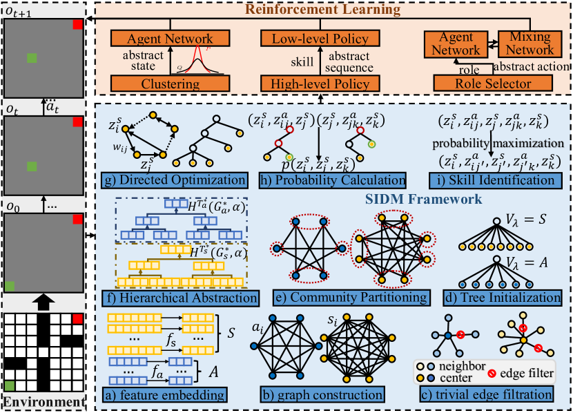
Figure 2: The details of structural information principles-based decision-making framework.

3.1 Graph Construction.

In our framework, we measure feature similarities between environmental observations and actions to construct two homogeneous graphs: a weighted, undirected, complete state graph, and a similarly structured action graph. To eliminate the negative interference caused by trivial weights, particularly those with absolute values near $0$, we apply edge filtration to both the state and action graphs.

To this end, we employ two encoder-decoder architectures [58] to acquire state and action representations, mapping the high-dimensional observations and original actions into two low-dimensional variables, $S$ and $A$ (step a in Figure 2). Within the encoders $f_{s}$ and $f_{a}$, each environmental observation and original action are embedded into feature representation $h_{s}$ for state $s\in S$ and $h_{a}$ for action $a$, respectively. For the purpose of illustrating the similarities between action functionalities and state transitions, we have designed two decoders, each with a distinct objectives, for decoding these embedded representations. In the state decoder, we implement the cross-entropy inverse objective [51] to predict the action $a$ between adjacent observations $o$ and $o^{\prime}$. Similarly, the action decoder processes each action representation $h_{a}$ and state representation $h_{s}$ to reconstruct the next observation $o^{\prime}$ and the environmental reward $r$. Considering the historical trajectories $\tau$, we aim to minimize the above decoding loss $\mathcal{L}_{de}$ to train the observation and action embedding models.

To better demonstrate our framework, we will reference the state graph $G_{s}$ as an example, while performing identical operations on the action graph $G_{a}$. In the graph $G_{s}$, each state $s\in S$, associated with an observations $o\in O$ in the trajectories $\tau$, is treated as a vertex $v\in V$. These vertices are interconnected, forming a complete graph (step b in Figure 2). For every distinct pair of states $s_{i}$ and $s_{j}$ where $i\neq j$, the feature similarity $\mathcal{C}_{s_{i},s_{j}}\in\left[-1,1\right]$ is measured through Pearson Correlation Analysis between their embedded representations $h_{s_{i}}$ and $h_{s_{j}}$, as outlined follows:

$$\mathcal{C}_{s_{i},s_{j}}=\frac{\mathbb{E}\left((h_{s_{i}}-\mu_{h_{s_{i}}})(h_{s_{j}}-\mu_{h_{s_{j}}})\right)}{\sigma_{h_{s_{i}}}\sigma_{h_{s_{j}}}}\text{,}$$ (5)

where $\mu_{h_{s_{i}}}$ and $\sigma_{h_{s_{i}}}$ denote the mean and variance of the state representation $h_{s_{i}}$. Intuitively, a higher absolute value of $\mathcal{C}_{s_{i},s_{j}}$ indicates a stronger similarity between states $s_{i}$ and $s_{j}$, which is taken into account during the subsequent state abstraction. The calculated similarity $\mathcal{C}_{s_{i},s_{j}}$ is then assigned as the weight $w_{ij}$ to the undirected edge $(s_{i},s_{j})$ in the graph $G_{s}$.

In the filtration for trivial edges in $G_{s}$, we minimize its one-dimensional structural entropy to simplify the complete state graph into a k-nearest neighbor (kNN) graph (step c in Figure 2). A lower one-dimensional structural entropy indicates more effective removal of noisy information from the complete graph. This filtration procedure is summarized in Algorithm 1. For a more sensitive filtration, we incorporate a modification factor $M$ to adjust the edge weights of $G_{s}$ (line 1 in Algorithm 1) as follows:

$$w_{ij}^{\prime}=w_{i,j}+M,\quad M=\frac{1}{2n}\cdot\frac{1}{m}\sum_{i,j}w_{ij}\text{.}$$ (6)

We take each state $s\in S$ as the center vertex, preserving only its $k$ edges with the highest absolute weights. Subsequently, we compute the one-dimensional structural entropy $H^{1}(G_{\text{k}})$ of the resulting kNN graph $G_{\text{k}}$ (lines 3 and 4 in Algorithm 1). We then assess the $H^{1}(G_{\text{k}})$ metric across a spectrum of plausible k values (line 2 in Algorithm 1) and select the optimal value $\text{k}^{*}$ that minimizes the one-dimensional structural entropy (Line 5 in Algorithm 1). The final output is the associated graph $G_{\text{k}^{*}}$, which serves as the sparse state graph $G^{*}_{s}$ (lines 6 and 7 in Algorithm 1).

Input: a weighted, undirected, and complete graph $G=(V,E,W)$

Output: the sparse graph $G^{*}$

1 $G^{\prime}\leftarrow$ reweight the graph $G$ via Equation 6

2 for $\text{k}=1,2,...,n-1$ do

3       $G_{\text{k}}\leftarrow$ construct the kNN graph

4       $H^{1}(G_{\text{k}})\leftarrow$ calculate the one-dimensional structural entropy of $G_{\text{k}}$ via Equation 1

5      

6$\text{k}^{*}\leftarrow\arg\min_{k}\{H^{1}(G_{\text{k}})\}$

7 $G^{*}\leftarrow G_{\text{k}^{*}}$

8 return $G^{*}$

Algorithm 1 The Edge Filtration Algorithm

3.2 Hierarchical Abstraction

To facilitate hierarchical state and action abstractions, we minimize the high-dimensional structural entropy of sparse graphs, thus completing the community partitioning for both states and actions. For each community, we design an aggregation function using assigned entropy as vertex weights to obtain its embedding, which are interpreted and represented as abstract states and actions in our work.

As shown step d in Figure 2, we initialize a one-layer encoding tree $T_{s}$ for the sparse graph $G^{*}_{s}$ as follows: 1) For the state variable $S$, we create a root node $\lambda$ with $V_{\lambda}=S$; 2) For each state $s\in S$, we create a leaf node $\nu$ as a child of the root $\lambda$, $\nu^{-}=\lambda$, and set $V_{\nu}=\{s\}$. The initial encoding tree $T_{s}$ depicts an initial partitioning structure of the state variable $S$, where each vertex community consists of only a single state.

To optimize the community partitioning of states further, we gradually reduce the structural entropy of $G_{s}^{*}$ under $T_{s}$, increasing the tree height from $1$ to $K$. The final $K$-layer encoding tree is the optimal encoding tree, thus representing the optimal partitioning structure. To enhance the stability of our optimization procedure, we have updated the operators from our previous works [31, 30] with two new optimization operators, stretch and compress, from the HCSE algorithm [29]. Within the encoding tree $T_{s}$, the stretch operator is defined over brother nodes sharing the same parent node, while the compress operator targets tree nodes at varying heights. Following a cycle of “stretch-compress” operations on the set $U^{s}_{i}$ of $i$-layer tree nodes in $T_{s}$, we characterize the average variation in structural entropy as $\overline{\operatorname{Spar}}_{i}(T_{s})$. Starting with the one-layer initial encoding tree, we greedily execute the “stretch-compress” cycles, aiming to reduce the $K$-dimensional structural entropy of $G_{s}^{*}$ until we reach the $k$-layer optimal encoding tree $T^{*}_{s}$.

This iterative optimization is summarized in Algorithm 2. During each iteration, we traverse all sets of tree nodes at the same level and select the set that most effectively decreases structural entropy (line 3 in Algorithm 2). These selected nodes then undergo a cycle of stretch-compress operations (lines 6-9 in Algorithm 2). When the tree height satisfies $h_{T}=K$ (line 2 in Algorithm 2) or no nodes set satisfies $\overline{\operatorname{Spar}}_{i^{*}}(T)>0$ (lines 4 and 5 in Algorithm 2), we terminate the iteration and output $T$ as the optimal encoding tree $T^{*}$ (lines 12 and 13 in Algorithm 2).

The tree $T^{*}_{s}$ epitomizes the optimal hierarchical partitioning of states $S$ (step e in Figure 2), where the root node $\lambda$ corresponds to $S$, $V_{\lambda}=S$, each leaf node $\nu$ corresponds to a singleton of a single state vertex $s\in S$, $V_{\nu}=\{s\}$, and other tree nodes correspond to various state subsets across different layers.

Input: The one-layer initial encoding tree $T$, $K\in\mathbb{Z}^{+}$

Output: The $K$-layer optimal encoding tree $T^{*}$

1 $h_{T}\leftarrow$ height of $T$

2 while $h_{T}<K$ do

3       $i^{*}\leftarrow\arg\max_{i}\{\overline{\operatorname{Spar}}_{i}(T)\}$

4       if $\overline{\operatorname{Spar}}_{i^{*}}(T)=0$ then

5             break

6      for $\alpha\in U_{i^{*}}$ do // stretch-compress

7             stretch($T_{\alpha}$)

8             compress($T_{\alpha}$)

9             $h_{T}\leftarrow h_{T}+1$

10      for $i=i^{*}+1,...,h_{T}$ do

11             update $U_{i}$

12      

13$T^{*}\leftarrow T$

return $T^{*}$

Algorithm 2 The Optimization Algorithm

According to the structural information principles, the entropy assigned to each tree node, as specified in Eq.2, measures the uncertainty of a single-step random walk reaching its associated vertex community from its parent’s community. This uncertainty is quantified as node weight, enabling the design of a hierarchical aggregation function (step f in Figure 2) to represent all nodes in the optimal encoding tree $T^{*}_{s}$. For each leaf node $\nu$ where $V_{\nu}={s}$, the $0$-level abstraction is defined using the encoder-decoder structure described in Section 3.1, resulting in the node representation $h_{\nu}=h_{s}$. For each non-leaf node $\alpha$, the softmax function is applied to normalize the weights of its children, and the representation $h_{\alpha}$ is calculated as follows:

$$h_{\alpha}=\sum_{i=1}^{L_{\alpha}}\frac{\exp\left({H^{T^{*}_{s}}\left(G^{*}_{s};\alpha^{\langle i\rangle}\right)}\right)}{\sum_{j=1}^{L_{\alpha}}\exp{\left({H^{T^{*}_{s}}\left(G^{*}_{s};\alpha^{\langle j\rangle}\right)}\right)}}\cdot h_{\alpha^{\langle i\rangle}}\text{,}$$ (7)

where the height of tree node $\alpha$ denotes the level of state abstraction for the state community $V_{\alpha}$. In our work, the default abstraction level is set to $K-1$. The hierarchical abstraction for the state variable $S$ and action variable $A$ are defined as the node sets $U^{s}_{K-1}$ and $U^{a}_{K-1}$, termed abstract states $Z_{s}$ and actions $Z_{a}$. The representations learned for nodes in $U_{K-1}$ capture the knowledge extracted from the original state and action variables.

3.3 Skill Identification

By analyzing abstract elements in historical trajectories, we transform heterogeneous environmental transitions, driven by multi-type actions, into homogeneous transitions between abstract states. To overcome the limitations of our previous studies’ undirected constraints [31, 30], we further define and optimize high-dimensional structural entropy for directed graphs for adaptive skill identification.

Taking the abstract states $Z_{s}$ as vertices, we create a homogeneous, weighted, directed graph $G_{dir}=(Z_{s},E_{dir},W_{dir})$ (step g in Figure 2). Directed edges $(z_{i}^{s},z_{j}^{s})\in E_{dir}$ are established between vertex pairs $z_{i}^{s}$ and $z_{j}^{s}$ if there is a original transition between their corresponding state subsets. For each edge $(z_{i}^{s},z_{j}^{s})$, its occurrence frequency is ascertained through analysis of all corresponding original transitions in $\tau$, which in turn establishes the edge weight $w_{ij}$. Regarding all actions in these original transitions, their collective parent node in $T^{*}_{a}$ is identified as an abstract action $z_{ij}^{a}$, resulting in the formation of an abstract transition $(z_{i}^{s},z_{ij}^{a},z_{j}^{s})$. Random directed edges are introduced into the graph $G_{dir}$ to guarantee its strong connectivity. Specifically, strongly connected components within $G_{dir}$ are identified, and directed edges between these components are established at a minimal probability to facilitate a circular layout. Subsequently, all edge weights are adjusted to ensure the sum of their weights equals $1$.

In this strongly connected transition graph, we compute the steady-state distribution $\operatorname{SD}$ for all vertices and define the one-dimensional structural entropy as follows:

$$H^{1}(G_{dir})=-\sum_{z_{i}^{s}\in Z_{s}}{\operatorname{SD}_{i}\cdot\log\operatorname{SD}_{i}}\text{,}$$ (8)

where $\operatorname{SD}_{i}$ is the distribution of vertex $z_{i}^{s}$. For each node $\alpha$ within the encoding tree $T$ of this graph, the assigned structural entropy is given by:

$$H^{T}(G_{dir};\alpha)=-\frac{g_{\alpha}}{vol(G_{dir})}\cdot\log\frac{\mathcal{V}_{\alpha}}{\mathcal{V}_{\alpha^{-}}}\text{,}$$ (9)

$$\mathcal{V}_{\alpha}=\sum_{z^{s}_{i}\in Z_{s}}\sum_{z^{s}_{j}\in V_{\alpha}}\frac{\operatorname{SD}_{i}\cdot w_{ij}}{\sum_{z^{s}_{k}\in Z_{s}}w_{kj}}\text{,}$$ (10)

$$g_{\alpha}=\sum_{z^{s}_{i}\notin V_{\alpha}}\sum_{z^{s}_{j}\in V_{\alpha}}\frac{\operatorname{SD}_{i}\cdot w_{ij}}{\sum_{z^{s}_{k}\in Z_{s}}w_{kj}}\text{.}$$ (11)

The $K$-dimensional structural entropy of $G_{dir}$ is defined as follows:

$$H^{T}(G_{dir})=\sum_{\alpha\in T}{H^{T}(G_{dir};\alpha)}\text{,}$$ (12)

$$H^{K}(G_{dir})=\min_{T}\left\{H^{T}(G_{dir})\right\}\text{.}$$ (13)

Expanding upon the merge and combine operators introduced by deDoc [56], we aim to reduce the $K$-dimensional structural entropy and summarize the optimization for directed graphs in Algorithm 3. In each iteration, we traverse all node pairs of identical height (lines 4 and 9 in Algorithm 3) and selectively execute either the merge or combine operator (lines 7 and 12 in Algorithm 3), based on which most significantly reduces the structural entropy (lines 5 and 10 in Algorithm 3), under the condition that the tree height remains below $K$ (line 2 in Algorithm 3). When no node pair satisfies $\Delta SE>0$ (line 15 in Algorithm 3), we terminate the iteration and output $T$ as the optimal encoding tree $T^{*}$ (lines 16 and 17 in Algorithm 3).

Input: The one-layer initial encoding tree $T$, $K\in\mathbb{Z}^{+}$

Output: The $K$-layer optimal encoding tree $T^{*}$

1 $h_{T}\leftarrow$ height of $T$

2 while $h_{T}<K$ do

3       $\Delta SE\leftarrow 0$

4       for each pair of nodes $\alpha_{0}$ and $\alpha_{1}$ in $T$ do

5             $\Delta SE,\alpha_{0}^{*},\alpha_{1}^{*}\leftarrow$ maximize the reduction of the structural entropy caused by the merge operator

6            

7      if $\Delta SE>0$ then

8             merge($\alpha_{0}^{*}$ and $\alpha_{1}^{*}$)

9             Continue

10            

11      for each pair of nodes $\alpha_{0}$ and $\alpha_{1}$ in $T$ do

12             $\Delta SE,\alpha_{0}^{*},\alpha_{1}^{*}\leftarrow$ maximize the reduction of the structural entropy caused by the combine operator

13            

14      if $\Delta SE>0$ then

15             combine($\alpha_{0}^{*}$ and $\alpha_{1}^{*}$)

16             Continue

17            

18      else

19             Break

20            

21      

22$T^{*}\leftarrow T$

23 return $T^{*}$

Algorithm 3 The Optimization Algorithm on Directed Graphs

For each abstract transition $(z_{i}^{s},z_{ij}^{a},z_{j}^{s})$, we denote the corresponding leaf nodes as $\nu_{i}$ and $\nu_{j}$, with $V_{\nu_{i}}=\{z_{i}^{s}\}$ and $V_{\nu_{i}}=\{z_{j}^{s}\}$. In the tree $T^{*}$, we locate the common parent node $\delta$ of these leaves and quantify the transition’s occurrence probability $p(z_{i}^{s},z_{j}^{s})$ (step h in Figure 2), as described below:

$$p(z_{i}^{s},z_{j}^{s})=\frac{\sum_{V_{\delta}\subseteq V_{\alpha}\subset V_{\lambda}}H^{T^{*}}(G_{dir};\alpha)}{\sum_{V_{\nu_{j}}\subseteq V_{\alpha}\subset V_{\lambda}}H^{T^{*}}(G_{dir};\alpha)}\text{.}$$ (14)

In a random walk across abstract states $Z_{s}$, the numerator quantifies the uncertainty of reaching either vertex $z_{i}^{s}$ or $z_{j}^{s}$, while the denominator quantifies the uncertainty of reaching vertex $z_{j}^{s}$. Consequently, a higher value of $p(z_{i}^{s},z_{j}^{s})$ signifies a reduced uncertainty in transitioning from vertex $z_{i}^{s}$ to $z_{j}^{s}$, thereby indicating the abstract transition $(z_{i}^{s},z_{ij}^{a},z_{j}^{s})$ with a greater occurrence probability. As shown step i in Figure 2, for each abstract transition $(z_{i}^{s},z_{ij}^{a},z_{j}^{s},z_{jk}^{a},z_{k}^{s})$ of length $2$, we evaluate all abstract states to replace the intermediate abstract state, with the objective of maximizing the occurrence probability, thus forming an optimized transition $(z_{i}^{s},z_{ij^{\prime}}^{a},z_{j^{\prime}}^{s},z_{j^{\prime}k}^{a},z_{k}^{s})$. This optimized abstract state-action sequence is then identified as a skill within our subsequent skill-based learning mechanism. To offset the loss of essential information due to sampling, we utilize the occurrence probability to reestablish the correlations between all pairs of abstract states. These reconstituted correlations are subsequently used as decoded targets in the calculation of structural information loss $\mathcal{L}_{si}$.

3.4 Abstract MDP

Through the hierarchical state abstraction, the original decision-making process is condensed into an abstract MDP, achieving a significant reduction in the number of states.

In the tree $T^{*}_{s}$, the node set $U^{s}_{K-1}$ is designated as the abstract state variable $Z_{s}$, where $Z_{s}=U^{s}_{K-1}$, thus forming an abstraction function $f\phi:S\rightarrow Z_{s}$. As shown in Figure 2, the SIDM maps each state $s_{i}\in S$ to an abstract state $z^{s}_{j}\in Z_{s}$, such that $s_{i}\in V_{\lambda^{\langle j\rangle}}$. The corresponding node $\lambda^{\langle j\rangle}$ is selected as the cluster center $c_{j}$ of the subset $V_{\lambda^{\langle j\rangle}}$, and their representations are used to compute a soft matrix $Q$, where $Q_{ij}$ indicates the likelihood of assigning state $s_{i}$ to cluster center $c_{j}$. Additionally, a high-confidence assignment matrix $P$ is derived from $Q$, and the Kullback-Lerbler (KL) divergence between $P$ and $Q$ is calculated, resulting in the clustering loss $\mathcal{L}_{clu}$ as follows:

$$\mathcal{L}_{clu}=KL(P\|Q)=\sum_{i}\sum_{j}P_{ij}\log\frac{P_{ij}}{Q_{ij}}\text{.}$$ (15)

This clustering loss $\mathcal{L}_{clu}$, combined with the decoding loss $\mathcal{L}_{de}$ and structural information loss $\mathcal{L}_{si}$, is minimized to optimize the hierarchical state abstract process in an end-to-end fashion.

3.5 Skill-based Learning

To alleviate the reliance on expert knowledge in skill-based RL, we leverage the skill identification to introduce a two-layer learning mechanism. This mechanism is designed to autonomously acquire general skills applicable across various downstream tasks.

Consistent with prior studies [119, 120], we utilize a variational autoencoder (VAE) [121] to embed all identified skills $\mathcal{K}$ into a latent space. The encoder simultaneously processes the entire abstract state-action sequence for each skill, while the decoder reconstructs individual abstract actions conditioned on the abstract states and skill embedding. Periodically, the high-level policy, $\pi_{h}:Z_{s}\times\mathcal{K}\mapsto[0,1]$, maps a particular abstract state $z_{i}^{s}\in Z_{s}$ to a skill embedding $\mathcal{K}_{i}\in\mathcal{K}$ and employs the decoder to reconstruct the abstract state-action sequence. In the skill horizon, the low-level policy, $\pi_{l}:Z_{s}\times\mathcal{K}_{i}\times Z_{a}\mapsto[0,1]$, adapt the decoded sequence at the actionable level, thus increasing the diversity of downstream tasks.

3.6 Role-based Learning.

To achieve effective and stable multi-agent collaboration in MARL, we utilize the hierarchical action abstraction to develop an automatic role-based learning mechanism.

In the cooperative multi-agent decision-making process $\mathcal{M}_{m}$, the SIDM processes all agents’ action-observation histories $\left[\tau_{i}\right]_{i=1}^{|\mathcal{N}|}$ and the joint reward $r$. It defines the node set $U^{a}_{K-1}$ in $T^{*}_{a}$ as the abstract actions $Z_{a}$ and discovered roles $\Psi$, where $\Psi=Z_{a}=U^{a}_{K-1}$. For each agent $n_{i}\in\mathcal{N}$, as depicted in Figure 2, the selector assigns a role $z_{j}^{a}\in Z_{a}$ and the corresponding action subset $V_{\lambda^{\langle j\rangle}}$. This allows the agent network to learn a role policy $\pi_{\rho_{j}}:\tau_{i}\times V_{\lambda^{\langle j\rangle}}\mapsto[0,1]$, avoiding substantial explorations in the joint state-action space. Agents sharing the same role $z^{a}_{j}$ focus on exploring the subset $V_{\lambda^{\langle j\rangle}}$ based on their individual observations, with the aim of jointly maximizing their team reward for subtask $t_{j}$. Furthermore, the SIDM is agnostic to special MARL algorithms and easily integrates various value function factorization methods into its policy networks. Taking inspiration from RODE [86], we also use QPLEX-style mixing networks [89] to coordinate the role assignment and policy learning of all agents.

3.7 Time Complexity Analysis

This section examines the time complexity of the SIDM framework, encompassing graph construction, hierarchical abstraction, and skill identification modules, to assess its practical applicability. The total time complexity of SIDM is denoted as $O(n^{2}+n+m\cdot\log^{2}n)$, where $n=|V|$ and $m=|E|$ indicate the quantities of vertices and edges in the respective state or action graph. Specifically, graph construction has a complexity of $O(n^{2}+n)$, attributable to $O(n^{2})$ for complete graph construction and $O(n)$ for filtering insignificant edges. According to the analysis [29], the optimization of a high-dimensional encoding tree through the stretch and compress operators incurs a complexity of $O(m\cdot\log^{2}n)$. The hierarchical abstraction of a $K$-layer optimal encoding tree with $n$ leaves has a proven upper bound of $O(n)$. Since the number of abstract states in the transition graph does not exceed $n$, the skill identification module’s time complexity is capped at $O(m\cdot\log^{2}n+n)$.

4 Experimental Setup

4.1 Datasets

To validate the effectiveness and efficiency of our SIDM framework, we have conducted extensive and comprehensive experiments in single-agent decision-making and multi-agent collaboration scenarios, incorporating both offline and online state abstractions in Abstract MDP, skill-based learning in DRL, and role-based learning in MARL. Additionally, within the SIDM framework, the state abstraction, skill-based learning, and role-based learning mechanisms are referred to as SISA, SISL, and SIRD, respectively.

4.1.1 Offline and Online State Abstractions

Initially, we assess the SISA mechanism for offline state abstraction within a visual gridworld environment. Mirroring experiments in Markov abstraction [51], each $(x,y)$ coordinate in the $6\times 6$ gridworld is associated with an image containing high-dimensional noise. During the offline training phase, the agent is exposed to these images, adopting a random exploration policy across four directional actions, devoid of any knowledge regarding the actual grid positions. When training the DQN policy network [35], the abstraction function mapping original images to state representations is fixed.

Subsequently, we explore the SISA in an online context, applying it to a challenging and diverse series of image-based continuous control tasks from the DeepMind Control Suite (DMControl) [61]. Specifically, our online abstraction experiments focus on nine DMControl tasks: $ball\_in\_cup$-$catch$, $cartpole$-$swingup$, $cheetah$-$run$, $finger$-$spin$, $reacher$-$easy$, $walker$-$walk$, $hopper$-$hop$, $hopper$-$stand$, and $pendulum$-$swingup$.

4.1.2 Skill-based Learning

In skill-based learning, we employ robotic control benchmarks, including the bipedal robot [75] and a $7$-Dof Fetch arm [114], executed in the MuJoCo physics simulator [112]. For the bipedal robot experiments, six diverse tasks are chosen, necessitating varied skills like jumping ($Hurdles$), torso control ($Limbo$), intricate foot manipulation ($Stairs$), and body balance ($PoleBalance$). In the context of the $7$-Dof fetching experiments, four downstream tasks, namely $Table$-$Cleanup$, $Slippery$-$Push$, $Pyramid$-$Stack$, and $Complex$-$Hock$, are selected. To underscore the significance of efficient exploration, all tasks are designed with sparse rewards, awarded solely upon achieving a goal or subgoal.

4.1.3 Role-based Learning

In the MARL subfield, we evaluate the SIRD mechanism using a mainstream benchmark of Centralized Training with Decentralized Execution (CTDE) algorithms with complex environments and high control complexity, specifically the StarCraft II micromanagement (SMAC) [84]. In these micromanagement scenarios, each agent autonomously manages an allied unit based on local observations, while the enemy units are directed by a built-in AI. At each time step, each agent selects an action from a discrete action space, which includes moving in four directions, stopping, taking no-op, and selecting an enemy/ally unit to attack/heal. The more demanding maps, classified as hard and super-hard, represent significant exploration challenges necessitating intricate collaborative strategies among agents. Given our objective to enhance multi-agent collaboration, our primary emphasis lies on performance on hard and super-hard maps.

4.2 Baselines

In the Abstract MDP subfield, we compare the SISA mechanism to various methods in offline and online settings. Offline comparisons include the pixel prediction method [59], reconstruction method [60], and Markov abstraction method [51]. Online, the SISA is contrasted with the random data augmentation method RAD [63], contrastive method CURL [49], bisimulation method DBC [50], pixel-reconstruction method SAC-AE [64], Markov abstraction method [51], data-augmented DrQv2 [117]. In the DRL subfield, our baselines consist of SOTA non-skill-based methods (SAC [62], BC+Fine-Tuning [115]), skill-based methods (HIRO [27], HIDIO [26], HSD-3 [75], PaRRot [116], SPiRL [8], Reskill [113]), and exploration improvement method Switching Ensemble [108]. In the MARL subfield, the baselines encompass independent Q-learning method IQL [93], value-based methods (VDN [88], QMIX [83], QPLEX [89], QTRAN [90]), actor-critic method COMA [91], bidirectional Q-learning ACE [118] and role-based method RODE [86].

4.3 Experimental Setting

In the proposed SIDM framework, the maximum height of encoding trees and the dimensionality of structural entropy are set to $3$, $K=3$, with a default hierarchical abstraction level of $2$. For the SISA mechanism, parameters include a latent dimension to $50$, a replay buffer size of $1e5$, the Adam optimizer, a batch size of $128$, and a discount factor to $0.99$. The Soft Actor-Critic (SAC) [62], utilized as the underlying RL algorithm, is integrated with various state abstraction methods. For the SISL mechanism, we employ the Adam optimizer, a replay buffer size of $1e6$, a mini-batch size of $256$, and a discount factor of $0.99$. All skill-based learning experiments use neural networks with $4$ hidden layers, skip connections, and ReLU activations. The HIRO methodology uses SAC for both its high- and low-level policies, termed HIRO-SAC. For the SIRD mechanism, the dimension of action representations is set to $20$, the optimizer to RMSprop with a learning rate of $0.0005$, the mixing network incorporates a $32$-dimensional hidden layer with ReLU activation, and the discount factor is $0.99$. All MARL experiments adhere to the SMAC benchmark’s default observation and reward settings. Experimental results are illustrated with the average value and standard deviation of performance conducted with ten random seeds to ensure robust evaluation.

4.4 Implementation

We implement the SISA mechanism with Python 3.8.15, Pytorch 1.13.0, the SISL mechanism with Python 3.9.1, Pytorch 1.9.0, and Tensorboard 1.15, and the SIRD mechanism with Python 3.5.2, Pytorch 1.5.1. All experiments are conducted on five Linux servers with GPU (NVIDIA RTX A6000) and CPU (3.00 GHz Intel i9-10980XE).

5 Evaluation and Discussion

5.1 State Abstraction Mechanism

Extensive empirical and comparative experiments are conducted to showcase the advantages of SISA mechanism, including both offline abstraction for a visual gridworld and online abstraction for continuous control tasks. To assess sample efficiency, we record the environmental steps required to attain specific reward targets for each method.

5.1.1 Offline Abstraction for Visual Gridworlds

In the visual gridworld domain, a navigation task is performed, and the learning curves of SISA and three other baselines are plotted in Figure 3. For a reference, we also include a learning curve labeled TrueState for DQN trained on ground-truth positions $(x,y)$ without any abstraction function. The convergence point for each curve is indicated in parentheses. As shown in Figure 3(left), the SISA reaches convergence at $76$ epochs with an average episode reward of -$7.17$, surpassing the baselines and equating to TrueState’s performance $(82,-7.31)$. Furthermore, Figure 3(right) depicts the $2$-D abstract representations of noisy images within the $6\times 6$ gridworld, highlighting ground-truth positions in varied colors. The hierarchical abstraction in SISA mechanism more effectively reconstructs the relative positioning of these ground truths compared to the baselines, thus confirming its superior performance in offline abstraction.

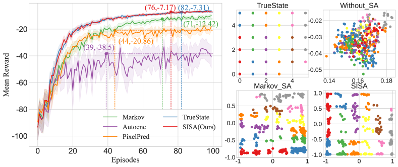
Figure 3: (left) Mean episode rewards for the navigation task in a visual gridworld. (right) Visualization of 2-D state abstractions for the $6\times 6$ visual gridworld domain.

5.1.2 Online Abstraction for Continuous Control

In our online experiments, all compared methods are evaluated across nine different continuous tasks from the DMControl suite. A summary of their mean episode rewards and deviations is provided in Table 2, excluding final rewards under $100.00$. To demonstrate the SISA’s effectiveness, we compare it against the SISA framework in our previous paper, referred to as SISA_pr in Table 2. Our results indicate that the SISA consistently outperforms other baselines across all DMControl tasks, showing a policy quality improvement of up to $25.02$ $(13.55\%)$. This is exemplified in the hopper-hop task, where the mean episode reward increases from $184.66$ to $209.68$. Moreover, the SISA exhibits greater stability compared to other methods, as evidenced by reduced standard deviations in six tasks and achieving the second or third lowest deviations in the remaining tasks, closely matching the top-performing baselines. This stability is attributed to SISA’s autonomous hierarchical state abstraction, guided by structural information principles.

Table 2: Summary of the mean episode rewards for different tasks from DMControl: “average value $\pm$ standard deviation” and “average improvement” (absolute value($\%$)). Bold: the best performance of our model, underline: the best performance among baselines.

Domain, Task	ball_in_cup-catch	cartpole-swingup	cheetah-run	finger-spin	reacher-easy
DBC	$168.95\pm 84.76$	$317.74\pm 77.49$	$432.24\pm 181.43$	$805.90\pm 78.85$	$191.44\pm 69.07$
SAC-AE	$929.24\pm 39.14$	$\underline{839.23}\pm 15.83$	$663.71\pm 9.16$	$898.08\pm 30.23$	$917.24\pm 38.33$
RAD	$\underline{937.97}\pm\underline{6.77}$	$825.62\pm\underline{9.80}$	$\underline{802.53}\pm 8.73$	$835.20\pm 93.26$	$908.24\pm\underline{25.62}$
CURL	$899.03\pm 30.61$	$824.46\pm 18.53$	$309.49\pm\underline{8.15}$	$949.57\pm 15.71$	$\underline{919.71}\pm 28.03$
Markov	$919.10\pm 38.14$	$814.94\pm 17.61$	$642.79\pm 65.92$	$\underline{969.91}\pm\underline{8.41}$	$806.34\pm 131.40$
DrQv2	$275.85\pm 44.87$	$573.10\pm 33.11$	$583.85\pm 11.52$	$629.23\pm 18.38$	$406.09\pm 66.09$
SISApr	$946.29\pm 8.63$	$858.21\pm 6.31$	$\textbf{806.67}\pm 8.61$	$\textbf{970.45}\pm 8.75$	$924.52\pm 19.04$
SISA	$\textbf{947.66}\pm\textbf{7.03}$	$\textbf{861.37}\pm\textbf{3.26}$	$803.32\pm\textbf{5.51}$	$968.59\pm\textbf{6.54}$	$\textbf{941.71}\pm\textbf{16.04}$
Abs.($\%$) Avg. $\uparrow$	$9.69(1.03)$	$22.14(2.64)$	$4.14(0.52)$	$0.54(0.06)$	$22.0(2.39)$
Domain, Task	walker-walk	hopper-hop	hopper-stand	pendulum-swingup	average reward
DBC	$331.97\pm 108.40$	-	-	$305.08\pm 86.78$	$284.55\pm 76.43$
SAC-AE	$895.33\pm 56.25$	-	-	-	$582.34\pm 25.07$
RAD	$907.08\pm 13.02$	$181.20\pm\underline{1.80}$	$\underline{891.87}\pm\underline{10.04}$	$\underline{843.84}\pm 8.99$	$\underline{792.61}\pm 19.78$
CURL	$885.03\pm\underline{9.88}$	-	-	-	$541.58\pm\underline{13.69}$
Markov	$\underline{918.44}\pm 12.58$	$\underline{184.66}\pm 6.48$	$864.70\pm 34.28$	$162.58\pm\underline{1.57}$	$698.16\pm 35.15$
DrQv2	$588.19\pm 11.13$	$84.43\pm 13.85$	$762.91\pm 11.31$	$821.35\pm 6.60$	$525.00\pm 24.10$
SISApr	$\textbf{921.64}\pm 12.43$	$209.55\pm 6.46$	$893.54\pm\textbf{4.74}$	$839.19\pm 7.90$	$818.90\pm 9.21$
SISA	$919.78\pm\textbf{9.40}$	$\textbf{209.68}\pm\textbf{6.23}$	$\textbf{900.45}\pm 5.05$	$\textbf{851.94}\pm\textbf{3.60}$	$\textbf{822.72}\pm\textbf{6.96}$
Abs.($\%$) Avg. $\uparrow$	$3.20(0.35)$	$25.02(13.55)$	$8.58(0.96)$	$8.1(0.96)$	$30.11(3.80)$

On the other hand, Figure 4 illustrates the sample-efficiency analysis for the DMControl experiments. In each task, the mean reward target is set to $0.9$ times the final policy quality achieved by SISA, and the strongest baseline is selected for comparison The SISA requires fewer steps to meet the mean episode reward target compared to classical baselines, thus exhibiting higher sample efficiency. Specifically, in the hopper-stand task, SISA shows a $64.86\%$ increase in sample efficiency, decreasing the required environmental steps from $222k$ to $78k$ to attain an episode reward of $810.405$.

Figure 4: The sample-efficiency results for DMControl tasks.

In conclusion, the SISA establishes remarkable performances in the DMControl domain, excelling in policy quality, stability, and sample efficiency during online learning with reward information. This success is attributed to the hierarchical state abstraction, which automatically balances between compressing irrelevant information and preserving essential characteristics, thereby securing these advantages. For each task, Figure 5 presents the learning curves of SISA and three leading baselines, showcasing the evolution of the mean episode reward over time and highlighting the points of convergence. Notably, in the pendulum-swingup task, the SISA achieves convergence after $320000.0$ timesteps and obtains an $851.94$ mean reward.

Figure 5: Mean episode rewards on DMControl environments.

5.2 Skill-based Learning Mechanism

In this subsection, we first pre-train the low-level policy in an empty environment and then train the high-level policy for each downstream task sharing the same pre-trained skills. For every ten environmental steps, we select a skill to execute based on the high-level policy.

In the bipedal robotic benchmark, we present the average values and standard deviations for the SISL mechanism and baselines after $1M$ environmental steps, as detailed in Table 3. Notably, in the $Hurdles$ task, the SISL method registers an increase of $2.1(18.75\%)$, elevating the average value from $11.2$ to $13.3$. These findings suggest the SISL mechanism’s capability to adapt skill selection in response to current environmental phases, successfully achieving the primary task without task-specific knowledge. A video demonstration of the skills applied in various episodes and environments is available on GitHub.

Table 3: Summary of the final performances after $1M$ steps across benchmark tasks with the bipedal robot: “average value $\pm$ standard deviation” and “average improvement” (absolute value($\%$)). Bold: the best performance un- der each category, underline: the second performance.

Method	Hurdles	Limbo	HurdlesLimbo	Stairs	Gaps	PoleBalance
SAC	$-0.1\pm 6.2$	$-0.1\pm\underline{0.2}$	$-0.1\pm 0.4$	$0.0\pm 4.8$	$-0.1\pm 0.5$	$231.5\pm 104.5$
Switching Ensemble	$-0.2\pm 3.0$	$-0.2\pm 4.3$	$-0.2\pm 3.6$	$1.1\pm 3.8$	$-0.2\pm 0.3$	$132.8\pm 230.1$
HIRO-SAC	$3.9\pm 1.6$	$1.1\pm 2.2$	$3.5\pm\underline{0.1}$	$0.0\pm\underline{0.0}$	$\underline{0.0}\pm\underline{0.2}$	$96.4\pm\underline{12.4}$
HIDIO	$-0.1\pm\textbf{0.1}$	$-0.1\pm\textbf{0.1}$	$-0.2\pm 0.1$	$-0.2\pm 0.3$	$-0.2\pm 0.3$	$117.6\pm 33.8$
HSD-3	$\underline{11.2}\pm 2.0$	$\underline{12.0}\pm 0.9$	$\underline{11.2}\pm 1.3$	$\underline{6.5}\pm 0.7$	$-0.2\pm 8.9$	$\underline{246.0}\pm 36.9$
SISL	$\textbf{13.3}\pm\underline{0.9}$	$\textbf{12.6}\pm 0.7$	$\textbf{12.8}\pm\textbf{0.1}$	$\textbf{7.0}\pm\underline{0.1}$	$\textbf{0.0}\pm\textbf{0.0}$	$\textbf{252.6}\pm\textbf{11.2}$
Abs.($\%$) Avg. $\uparrow$	$2.1(18.75)$	$0.6(5.0)$	$1.6(14.29)$	$0.5(7.69)$	$0.0(0.0)$	$6.6(2.68)$

For the $7$-DoF fetching benchmark, we conducted a comparative analysis of the SISL and several state-of-the-art RL methods, focusing on those operating in either the original action space (PARROT) or the skill space (SPiRL and Reskill). The average values and standard deviations of their final performances across tasks are summarized in Table 4. The SISL notably outperforms other baselines in all four tasks, with a maximum improvement of $32.70\%$ observed in the Slippery Push task. Regarding policy stability, the SISL exhibits minimal deviation in the Complex Hook task and nearly minimal deviations in the remaining three tasks, closely trailing the top-performing baseline. This superiority is attributed to the skill identification mechanism that leverages hierarchical state and action abstractions, ensuring an effective and versatile skill set for skill-based learning. The progression of their learning is depicted in Figure 6.

Table 4: Summary of the final performances across benchmark tasks with the $7$-DOF robotic arms: “average value $\pm$ standard deviation” and “average improvement” (absolute value($\%$)). Bold: the best performance in each task, underline: the second performance.

Method	Fetch Table Cleanup	Fetch Slippery Push	Fetch Pyramid Stack	Fetch Complex Hock
SPiRL	$11.33\pm 1.74$	$8.89\pm 2.92$	-	$33.65\pm 3.34$
BC + Fine-Tuning	-	$14.81\pm 2.91$	$15.43\pm 2.03$	-
PARROT	-	$32.10\pm 3.58$	$8.46\pm 3.54$	$13.07\pm 2.89$
Reskill	$\underline{35.48}\pm 0.39$	$\underline{42.42}\pm 1.32$	$\underline{16.91}\pm 1.68$	$\underline{58.93}\pm 0.34$
SISL	$\textbf{39.80}\pm 0.71$	$\textbf{56.29}\pm 1.43$	$\textbf{22.20}\pm 1.77$	$\textbf{67.06}\pm 0.13$
Abs.($\%$) Avg. $\uparrow$	$4.32(12.18)$	$13.87(32.70)$	$5.29(31.28)$	$8.13(13.80)$

Figure 6: Mean episode rewards across benchmark tasks with the $7$-DOF robotic arms.

5.3 Role-based Learning Mechanism

In this subsection, we compare the SIRD mechanism with state-of-the-art MARL algorithms using the SMAC benchmark’s easy, hard, and super hard map categories. We denote our proposed SIRD in our prior work as ’SIRD_pr’. Table 5 summarizes the comparative results, highlighting performances above $10.00\%$ and their deviations in each map category. Our SIRD mechanism outperforms baseline algorithms with an improvement of up to $6.66\%$ in average value and a decrease of up to $88.26\%$ in deviation, which are indicative of its performance advantages on policy quality and stability. The action abstraction based on the structural information principles enable automatic and effective role discovery, promoting cooperative abilities among agents and eliminating dependence on sensitive hyperparameters. These improvements are particularly notable in hard-exploration scenarios, such as on hard and super-hard maps.

Table 5: Summary of the test win rates under different map categories: “average value $\pm$ standard deviation” and “improvements/reductions” ((absolute value($\%$))). Bold: the best performance of our model, underline: the best performance among baselines.

Categories	Easy	Hard	Super Hard
COMA	$16.67\pm 22.73$	-	-
IQL	$52.50\pm 40.69$	$73.44\pm 24.85$	$10.55\pm 18.49$
VDN	$85.01\pm 17.22$	$71.49\pm 18.78$	$71.10\pm 27.23$
QMIX	$\underline{98.44}$ $\pm$ $\underline{2.10}$	$87.11\pm 18.58$	$70.31\pm 38.65$
QTRAN	$64.69\pm 36.79$	$58.20\pm 45.37$	$16.80\pm 20.61$
QPLEX	$96.88\pm 5.04$	$89.85$ $\pm$ $\underline{11.35}$	$84.77\pm 10.76$
MAPPO	$66.67\pm 35.35$	$61.72$ $\pm$ $23.60$	$73.98\pm 16.45$
RODE	$93.47\pm 10.19$	$88.44\pm 20.96$	$\underline{92.71}$ $\pm$ $\underline{9.20}$
ACE	-	$\underline{91.10}\pm 11.66$	$88.15\pm 5.21$
SIRDpr	$98.61\pm\textbf{1.75}$	$95.31\pm 6.63$	$95.71\pm 3.10$
SIRD	$\textbf{98.83}\pm 2.17$	$\textbf{95.83}\pm\textbf{4.99}$	$\textbf{97.50}\pm\textbf{1.08}$
Abs.($\%$) Avg. $\uparrow$	$0.39(0.40)$	$4.73(5.19)$	$4.79(5.17)$
Abs.($\%$) Dev. $\downarrow$	$0.35(16.67)$	$6.36(56.04)$	$8.12(88.26)$

Furthermore, we compare the SIRD mechanism with baseline algorithms across all $14$ SMAC maps to demonstrate their overall performance. Figure 7 displays the average test win rate and the number of maps where each MARL algorithm performs best at different stages of policy learning. As Figure 7(left) illustrates, the SIRD not only shows superior overall performance but also achieves faster convergence compared to the baselines. Remarkably, the SIRD maintains the highest average test win rate throughout the last $60\%$ of the learning process until achieving a final win rate of $96.7\%$, which exceeds the second-best (ACE at $92.73\%$) and the third-best (QPLEX at $90.99\%$) by $3.97\%$ and $5.71\%$, respectively. This enhanced performance, particularly in policy quality and learning efficiency, stems from effective exploration within the identified action subsets. Figure 7(right) reveals that SIRD secures the best final policy in almost half the maps ($6$ out of $14$), significantly surpassing the baselines.

Figure 7: (left)The average test win rates across all 14 maps; (right)the number of maps (out of 14) where the algorithm’s average test win rate is the highest.

The SIRD mechanism excels in policy quality and stability, establishing a new benchmark in state-of-the-art performance on the SMAC. For most SMAC tasks, we showcase the top four algorithms by plotting their learning curves in Figure 8. This includes the convergence point and associated variance for each algorithm. In the MMM$2$ task, as depicted in Figure 8, the SIRD converges at $1604442$ timesteps, achieving an impressive average win rate of $96.2\%$ with a low variance of $0.0036$. Furthermore, Figure 9 illustrates the SIRD-driven multi-agent collaboration in the $1$c$3$s$5$z task, highlighting dynamic role discovery and assignment throughout an episode.

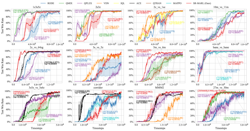
Figure 8: Average test win rates on SMAC maps.

Figure 9: The multi-agent collaboration based on the SIRD mechanism.

5.4 Generality Abilities

The proposed SIDM is a general framework and can be flexibly integrated with various single-agent and multi-agent RL algorithms to enhance their performances.

In the single-agent context, we incorporate our SISA mechanism with Markov abstraction and SAC-AE algorithms to develop the Markov-SISA and SAC-SISA variants, respectively. We assess their effectiveness on tasks ball_in_cup-catch and cartpole-swingup, finding each integration surpasses the original methods in policy quality and sample efficiency, as illustrated in Figure 10. These comparisons show the framework’s exceptional capacity for enhancing existing single-agent RL algorithms.

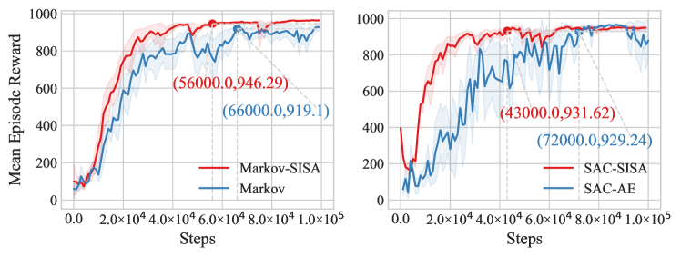
((a)) ball_in_cup-catch

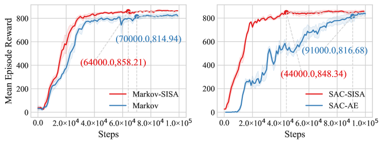
((b)) cartpole-swingup

Figure 10: Mean episode rewards of the SISA integrated with abstraction methods Markov and SAC-AE.

In the multi-agent context, the SIRD mechanism is integrated with the QMIX and QPLEX methods, yielding the SI-QMIX and SI-QPLEX variants. Figure 11 illustrates that these integrated methods surpass their original counterparts in policy quality, stability, and sample efficiency in tests on the $2$c_vs_$64$zg and MMM$2$ maps. These experimental outcomes indicate that the application of structural information principles for role discovery notably enhances multi-agent coordination.

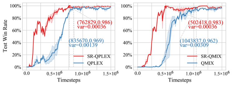
((a)) $2$c_vs_$64$zg

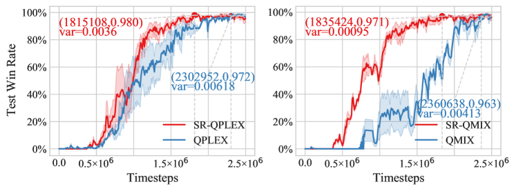
((b)) MMM$2$

Figure 11: Average test win rates of the SR-MARL integrated with value decomposition methods QMIX and QPLEX.

5.5 Ablation Experiments

In single-agent scenarios, we carry out experiments on the $ball\_in\_cup$-$catch$ and $finger$-$spin$ tasks through ablation studies to understand the functions of the clustering loss $\mathcal{L}_{clu}$ and structural information loss $\mathcal{L}_{si}$. We develop two variants of SISA: SISA-PD and SISA-CR, by removing probability distribution in Section 3.4 and correlation reconstruction in Section 3.3. As shown in Figure 12, SISA outperforms both SISA-PD and SISA-CR in terms of policy quality, stability, and sample efficiency. These significant results indicate that both the clustering loss and structural information loss are crucial for the hierarchical state abstraction, thereby guaranteeing the performance advantages of SISA.

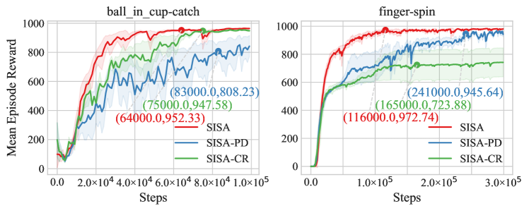
Figure 12: Mean rewards for ablation studies in SISA.

In multi-agent scenaros, we conduct ablation studies to assess the significance of the graph construction and edge filtration steps in achieving performance advantages on $2$c_vs_$64$zg and $1$c$3$s$5$z maps. Two variants, SIRD-ST and SIRD-SP, are developed as degenerated models of the SIRD without specfic functional modules. In the SIRD-ST variant, roles are identified from the joint action space using K-Means clustering. And the SIRD-SP variant directly optimizes the encoding tree of the complete action graph for role discovery. Figure 13 shows that SIRD outperforms SIRD-ST significantly in terms of the average and deviation of test win rates, indicating that the graph construction is crucial for the policy quality and stability of SIRD. On the other hand, the comparison between SIRD and SIRD-SP suggests that the edge filtration considerably boosts the learning process without affecting the performance advantages.

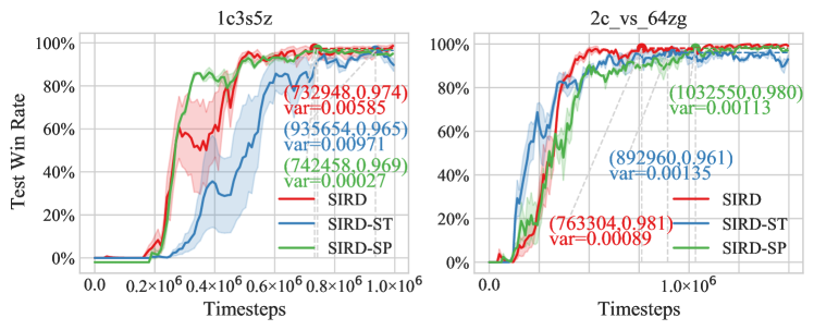
Figure 13: Average test win rates for ablation studies in SIRD.

In this section, we also explore different maximum heights of the encoding tree ($2$ and $3$) and name the associated variants SIRD-$2$ and SIRD-$3$. Their learning curves on two different maps ($2$c_vs_$64$zg and MMM$2$) are illustrated in Figure 14. We compare the policy quality, stability, and sample efficiency of these variants and find that SIRD-$3$ is more effective on the super hard map MMM$2$ while SIRD-$2$ performs better on the hard map $2$c_vs_$64$zg. This is because complex multi-agent collaboration on super hard maps requires a more hierarchical action space abstraction, which can be achieved using a higher encoding tree.

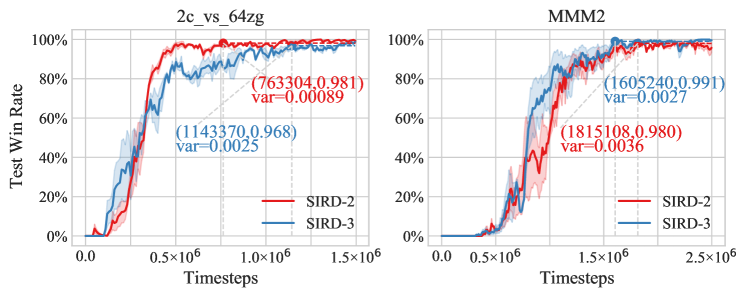
Figure 14: Average test win rates of the SIRD with the optimal encoding trees of different maximal heights ($2$ and $3$) on $2$c_vs_$64$zg and MMM$2$ maps.

6 Related Work

Structural Information Principles. The first metric of structural information was first proposed in 2016 [54], including formal definitions of structural entropy and partitioning tree. Structural entropy measures the dynamical complexity of networks and provides the principle of detecting the natural hierarchical structure called the partitioning tree. The one-dimensional structural entropy minimization principle was then proposed to construct cell sample networks and identify subtypes of cancer cells [55]. And deDoc utilizes ultra-low resolution Hi-C data to decode topologically associating domains by minimizing the K-dimensional structural entropy [56]. Afterward, the structural information principles have been widely applied to various domains. In 2019, a community-based structural entropy was defined to quantify the information amount revealed by a community for solving community deception problems [65]. In 2022, SEP [66] leveraged structural entropy to tackle local structure damage and suboptimal problem in hierarchical pooling approaches for superior performance on node classification.

State Abstraction for DRL. The SAC-AE [64] trains models to perfectly reproduce original states through pixel prediction and related tasks. In contrast, the CURL [49] uses differentiation to learn abstraction by determining if two augmented views are from the same observation. The DBC [50] takes an end-to-end approach by training a transition model and reward function to learn approximate bisimulation abstractions where equivalent original states have the same expected reward and transition dynamics. SimSR [68] uses a stochastic approximation method to learn abstraction from observations into robust latent representations. Meanwhile, IAEM [69] captures action invariance to efficiently obtain abstract representations. Allen et al. [51] introduce sufficient conditions for learning Markov abstract state representations, balancing the elimination of irrelevant details with the preservation of essential information. However, critical information loss inevitably occurs due to random sampling from finite replay buffers, which can impair performance on complex tasks. To address this, our SIDM Framework transforms heterogeneous transitions between environmental states into homogeneous transitions between abstract states and reconstructs correlations between pairs of abstract states (Equation 14) to compensate for this information loss induced by finite sampling.

Hierarchical Reinforcement Learning. The success of macro-operators and abstraction in classic planning systems [15, 14] has inspired hierarchical approaches to reinforcement learning [13, 12, 27], offering benefits such as improved exploration capabilities and easier individual learning problems. Such approaches enable the separate acquisition of low-level policies (skills) that can accelerate downstream task learning, with various methods proposed for discovering these primitives via random walk [11], mutual information objectives [109, 10], expertly traces [9, 8], and pre-training tasks [7, 6]. However, a trade-off between generality and specificity arises when low-level skills need to be useful across various tasks. Prior work on option discovery and hierarchical reinforcement learning has mostly favored specificity, choosing navigation problems in grid-world mazes [1, 5] or similar environments [109, 9] as benchmarks.

Role-based Learning. In natural systems [104, 103, 102], the role played by individuals is closely tied to labor division and efficiency improvement. To replicate these benefits, multi-agent systems decompose tasks and assign specialized agents to subtasks based on their roles, which reduces design complexity [105, 98]. However, the practical implementation of these approaches is limited by the fact that predefined task decomposition and roles may not be available [99, 2]. Bayesian inference has been introduced MARL algorithms to learn roles [100], and the Role-based Objectives with Emergent Specialization (ROMA) methodology encourage the emergence of roles by designing a specialization objective [85]. However, searching through the entire state-action space can make these methods inefficient. The Role Discovery by Decomposition of Joint Actions (RODE) method is proposed to address the above issue by decomposing the joint action spaces [86]. Nevertheless, the effectiveness of RODE is greatly influenced by practical knowledge as it is exceptionally sensitive to the parameters of the utilized clustering algorithms. The SIDM framework leverages structural information principles to generate action communities and define an aggregation function, facilitating hierarchical action abstraction. This approach enables an adaptive, effective, and stable role-based learning mechanism without the need for manual assistance.

Multi-Agent Reinforcement Learning. Multi-agent learning has the potential to model diverse and difficult tasks [84, 24, 23]. It can also enhance the understanding of real-world phenomena, such as tool usage [42], social influence [22], and inequity aversion [21]. Centralized learning on joint action space can avoid non-stationarity during learning but may not be scalable to large-scale problems. Promising approaches that exploit coordination independencies between agents include the coordination graph method [20] and value function decomposition methods [88, 83, 90, 89]. The latter avoids the need for pre-supplied dependencies between agents. Multi-agent policy gradient algorithms [82, 16] are stable and have strong theoretical convergence properties. These algorithms hold promise for extending MARL to continuous control problems. CCDA paradigms, such as COMA [91] and MADDPG [19], have been extended with recursive reasoning and attention mechanisms by PR2 [18] and MAAC [17], respectively.

7 Conclusion

This paper proposes a effective and general structural information principles-based decision-making framework (SIDM) from the information-theoretic perspective. A novel structural entropy-based aggregation function over tree nodes is designed to achieve hierarchical state and action abstractions for efficient exploration. Through extracting homogeneous transitions between abstract states, we calculate the common path entropy and introduce an innovative two-layer skill-based learning mechanism, independent of expert knowledge. Evaluations under challenging single- and multi-agent scenarios demonstrate that SIDM significantly and consistently improves policy quality, stability, and sample efficiency. Looking ahead, we plan to expand the encoding tree height and the structural entropy dimensionality, and to incorporate additional complex environments for enhanced performance evaluation. Moreover, it is also promising to study hierarchical state-action abstraction on the optimal encoding tree.

References

- [1] T. G. Dietterich, Hierarchical reinforcement learning with the maxq value function decomposition, JAIR 13 (2000) 227–303.
- [2] C. Sun, W. Liu, L. Dong, Reinforcement learning with task decomposition for cooperative multiagent systems, TNNLS 32 (5) (2020) 2054–2065.
- [3] H. Hasselt, Double q-learning, NeurIPS 23 (2010).
- [4] G. A. Rummery, M. Niranjan, On-line Q-learning using connectionist systems, Vol. 37, University of Cambridge, Department of Engineering Cambridge, UK, 1994.
- [5] R. S. Sutton, D. Precup, S. Singh, Between mdps and semi-mdps: A framework for temporal abstraction in reinforcement learning, AI 112 (1-2) (1999) 181–211.
- [6] K. Marino, A. Gupta, R. Fergus, A. Szlam, Hierarchical rl using an ensemble of proprioceptive periodic policies, in: ICLR, 2019.
- [7] C. Florensa, Y. Duan, P. Abbeel, Stochastic neural networks for hierarchical reinforcement learning, in: ICLR, 2017.
- [8] K. Pertsch, Y. Lee, J. Lim, Accelerating reinforcement learning with learned skill priors, in: CoRL, PMLR, 2021, pp. 188–204.
- [9] A. Ajay, A. Kumar, P. Agrawal, S. Levine, O. Nachum, Opal: Offline primitive discovery for accelerating offline reinforcement learning, in: ICLR, 2020.
- [10] A. Sharma, S. Gu, S. Levine, V. Kumar, K. Hausman, Dynamics-aware unsupervised discovery of skills, in: ICLR, 2019.
- [11] M. C. Machado, M. G. Bellemare, M. Bowling, A laplacian framework for option discovery in reinforcement learning, in: ICML, PMLR, 2017, pp. 2295–2304.
- [12] M. Riedmiller, R. Hafner, T. Lampe, M. Neunert, J. Degrave, T. Wiele, V. Mnih, N. Heess, J. T. Springenberg, Learning by playing solving sparse reward tasks from scratch, in: ICML, PMLR, 2018, pp. 4344–4353.
- [13] P. Dayan, G. E. Hinton, Feudal reinforcement learning, NeurIPS 5 (1992).
- [14] E. D. Sacerdoti, Planning in a hierarchy of abstraction spaces, AI 5 (2) (1974) 115–135.
- [15] R. E. Fikes, P. E. Hart, N. J. Nilsson, Learning and executing generalized robot plans, AI 3 (1972) 251–288.
- [16] J. Wang, Z. Ren, B. Han, J. Ye, C. Zhang, Towards understanding linear value decomposition in cooperative multi-agent q-learning (2020).
- [17] S. Iqbal, F. Sha, Actor-attention-critic for multi-agent reinforcement learning, in: ICML, PMLR, 2019, pp. 2961–2970.
- [18] Y. Wen, Y. Yang, R. Luo, J. Wang, W. Pan, Probabilistic recursive reasoning for multi-agent reinforcement learning, ArXiv Preprint ArXiv:1901.09207 (2019).
- [19] R. Lowe, Y. I. Wu, A. Tamar, J. Harb, O. Pieter Abbeel, I. Mordatch, Multi-agent actor-critic for mixed cooperative-competitive environments, NeurIPS 30 (2017).
- [20] W. Böhmer, V. Kurin, S. Whiteson, Deep coordination graphs, in: ICML, PMLR, 2020, pp. 980–991.
- [21] E. Hughes, J. Z. Leibo, M. Phillips, K. Tuyls, E. Dueñez-Guzman, A. García Castañeda, I. Dunning, T. Zhu, K. McKee, R. Koster, et al., Inequity aversion improves cooperation in intertemporal social dilemmas, NeurIPS 31 (2018).
- [22] N. Jaques, A. Lazaridou, E. Hughes, C. Gulcehre, P. Ortega, D. Strouse, J. Z. Leibo, N. De Freitas, Social influence as intrinsic motivation for multi-agent deep reinforcement learning, in: ICML, PMLR, 2019, pp. 3040–3049.
- [23] M. Jaderberg, W. M. Czarnecki, I. Dunning, L. Marris, G. Lever, A. G. Castaneda, C. Beattie, N. C. Rabinowitz, A. S. Morcos, A. Ruderman, et al., Human-level performance in 3d multiplayer games with population-based reinforcement learning, Science 364 (6443) (2019) 859–865.
- [24] O. Vinyals, I. Babuschkin, W. M. Czarnecki, M. Mathieu, A. Dudzik, J. Chung, D. H. Choi, R. Powell, T. Ewalds, P. Georgiev, et al., Grandmaster level in starcraft ii using multi-agent reinforcement learning, Nature 575 (7782) (2019) 350–354.
- [25] F. Belardinelli, A. Ferrando, V. Malvone, An abstraction-refinement framework for verifying strategic properties in multi-agent systems with imperfect information, AI (2023) 103847.
- [26] J. Zhang, H. Yu, W. Xu, Hierarchical reinforcement learning by discovering intrinsic options, in: ICLR, 2021.
- [27] O. Nachum, S. S. Gu, H. Lee, S. Levine, Data-efficient hierarchical reinforcement learning, NeurIPS 31 (2018).
- [28] C. E. Shannon, A mathematical theory of communication, BSTJ 27 (3) (1948) 379–423.
- [29] Y. Pan, F. Zheng, B. Fan, An information-theoretic perspective of hierarchical clustering, ArXiv Preprint ArXiv:2108.06036 (2021).
- [30] X. Zeng, H. Peng, A. Li, C. Liu, L. He, P. S. Yu, Hierarchical state abstraction based on structural information principles, ArXiv Preprint ArXiv:2304.12000 (2023).
- [31] X. Zeng, H. Peng, A. Li, Effective and stable role-based multi-agent collaboration by structural information principles, ArXiv Preprint ArXiv:2304.00755 (2023).
- [32] R. S. Sutton, A. G. Barto, et al., Introduction to reinforcement learning, Vol. 135, MIT Press Cambridge, 1998.
- [33] Y. LeCun, Y. Bengio, G. Hinton, Deep learning, Nature 521 (7553) (2015) 436–444.
- [34] J. Schmidhuber, Deep learning in neural networks: An overview, Neural Networks 61 (2015) 85–117.
- [35] V. Mnih, K. Kavukcuoglu, D. Silver, A. A. Rusu, J. Veness, M. G. Bellemare, A. Graves, M. Riedmiller, A. K. Fidjeland, G. Ostrovski, et al., Human-level control through deep reinforcement learning, Nature 518 (7540) (2015) 529–533.
- [36] K. Arulkumaran, M. P. Deisenroth, M. Brundage, A. A. Bharath, Deep reinforcement learning: A brief survey, SPM 34 (6) (2017) 26–38.
- [37] V. Mnih, A. P. Badia, M. Mirza, A. Graves, T. Lillicrap, T. Harley, D. Silver, K. Kavukcuoglu, Asynchronous methods for deep reinforcement learning, in: ICML, PMLR, 2016, pp. 1928–1937.
- [38] M. Jin, Z. Ma, K. Jin, H. H. Zhuo, C. Chen, C. Yu, Creativity of ai: Automatic symbolic option discovery for facilitating deep reinforcement learning, in: AAAI, Vol. 36, 2022, pp. 7042–7050.
- [39] S. Collins, A. Ruina, R. Tedrake, M. Wisse, Efficient bipedal robots based on passive-dynamic walkers, Science 307 (5712) (2005) 1082–1085.
- [40] E. Ie, V. Jain, J. Wang, S. Narvekar, R. Agarwal, R. Wu, H.-T. Cheng, T. Chandra, C. Boutilier, Slateq: A tractable decomposition for reinforcement learning with recommendation sets, in: IJCAI, International Joint Conferences on AI Organization, 2019, pp. 2592–2599.
- [41] C. Zhang, V. R. Lesser, Coordinated multi-agent reinforcement learning in networked distributed pomdps, in: AAAI, 2011, pp. 764–770.
- [42] B. Baker, I. Kanitscheider, T. M. Markov, Y. Wu, G. Powell, B. McGrew, I. Mordatch, Emergent tool use from multi-agent autocurricula, in: ICLR, 2020, pp. 1–28.
- [43] D. Andre, S. J. Russell, State abstraction for programmable reinforcement learning agents, in: AAAI, 2002, pp. 119–125.
- [44] N. K. Jong, P. Stone, State abstraction discovery from irrelevant state variables., in: IJCAI, Vol. 8, Citeseer, 2005, pp. 752–757.
- [45] D. Abel, D. Hershkowitz, M. Littman, Near optimal behavior via approximate state abstraction, in: ICML, PMLR, 2016, pp. 2915–2923.
- [46] M. Hutter, Extreme state aggregation beyond markov decision processes, TCS 650 (2016) 73–91.
- [47] D. Abel, D. Arumugam, L. Lehnert, M. Littman, State abstractions for lifelong reinforcement learning, in: ICML, PMLR, 2018, pp. 10–19.
- [48] C. Gelada, S. Kumar, J. Buckman, O. Nachum, M. G. Bellemare, Deepmdp: Learning continuous latent space models for representation learning, in: ICML, PMLR, 2019, pp. 2170–2179.
- [49] M. Laskin, A. Srinivas, P. Abbeel, Curl: Contrastive unsupervised representations for reinforcement learning, in: ICML, PMLR, 2020, pp. 5639–5650.
- [50] A. Zhang, R. T. McAllister, R. Calandra, Y. Gal, S. Levine, Learning invariant representations for reinforcement learning without reconstruction, in: ICLR, 2020.
- [51] C. Allen, N. Parikh, O. Gottesman, G. Konidaris, Learning markov state abstractions for deep reinforcement learning, NeurIPS 34 (2021) 8229–8241.
- [52] D. Abel, D. Arumugam, K. Asadi, Y. Jinnai, M. L. Littman, L. L. Wong, State abstraction as compression in apprenticeship learning, in: AAAI, Vol. 33, 2019, pp. 3134–3142.
- [53] C. Shannon, The lattice theory of information, TIT 1 (1) (1953) 105–107.
- [54] A. Li, Y. Pan, Structural information and dynamical complexity of networks, TIT 62 (6) (2016) 3290–3339.
- [55] A. Li, X. Yin, Y. Pan, Three-dimensional gene map of cancer cell types: Structural entropy minimisation principle for defining tumour subtypes, Scientific Reports 6 (2016) 1–26.
- [56] A. Li, X. Yin, B. Xu, D. Wang, J. Han, Y. Wei, Y. Deng, Y. Xiong, Z. Zhang, Decoding topologically associating domains with ultra-low resolution hi-c data by graph structural entropy, Nature Communications 9 (2018) 1–12.
- [57] R. Bellman, A markovian decision process, JMM (1957) 679–684.
- [58] K. Cho, B. V. Merriënboer, C. Gulcehre, D. Bahdanau, F. Bougares, H. Schwenk, Y. Bengio, Learning phrase representations using rnn encoder-decoder for statistical machine translation, in: EMNLP, 2014, pp. 1724–1734.
- [59] Ł. Kaiser, M. Babaeizadeh, P. Miłos, B. Osiński, R. H. Campbell, K. Czechowski, D. Erhan, C. Finn, P. Kozakowski, S. Levine, et al., Model based reinforcement learning for atari, in: ICLR, 2019.
- [60] A. X. Lee, A. Nagabandi, P. Abbeel, S. Levine, Stochastic latent actor-critic: Deep reinforcement learning with a latent variable model, NeurIPS 33 (2020) 741–752.
- [61] S. Tunyasuvunakool, A. Muldal, Y. Doron, S. Liu, S. Bohez, J. Merel, T. Erez, T. Lillicrap, N. Heess, Y. Tassa, dm_control: Software and tasks for continuous control, Software Impacts 6 (2020) 100022.
- [62] T. Haarnoja, A. Zhou, P. Abbeel, S. Levine, Soft actor-critic: Off-policy maximum entropy deep reinforcement learning with a stochastic actor, in: ICML, PMLR, 2018, pp. 1861–1870.
- [63] M. Laskin, K. Lee, A. Stooke, L. Pinto, P. Abbeel, A. Srinivas, Reinforcement learning with augmented data, NeurIPS 33 (2020) 19884–19895.
- [64] D. Yarats, A. Zhang, I. Kostrikov, B. Amos, J. Pineau, R. Fergus, Improving sample efficiency in model-free reinforcement learning from images, in: AAAI, Vol. 35, 2021, pp. 10674–10681.
- [65] Y. Liu, J. Liu, Z. Zhang, L. Zhu, A. Li, Rem: From structural entropy to community structure deception, NeurIPS 32 (2019).
- [66] J. Wu, X. Chen, K. Xu, S. Li, Structural entropy guided graph hierarchical pooling, in: ICML, PMLR, 2022, pp. 24017–24030.
- [67] J. Wu, S. Li, J. Li, Y. Pan, K. Xu, A simple yet effective method for graph classification, IJCAI (2022).
- [68] H. Zang, X. Li, M. Wang, Simsr: Simple distance-based state representations for deep reinforcement learning, in: AAAI, Vol. 36, 2022, pp. 8997–9005.
- [69] Z.-M. Zhu, S. Jiang, Y.-R. Liu, Y. Yu, K. Zhang, Invariant action effect model for reinforcement learning, in: AAAI, Vol. 36, 2022, pp. 9260–9268.
- [70] L. Illanes, X. Yan, R. T. Icarte, S. A. McIlraith, Symbolic plans as high-level instructions for reinforcement learning, in: ICAPS, Vol. 30, 2020, pp. 540–550.
- [71] J. Lee, M. Katz, D. J. Agravante, M. Liu, T. Klinger, M. Campbell, S. Sohrabi, G. Tesauro, Ai planning annotation in reinforcement learning: Options and beyond, in: ICAPS, 2021.
- [72] Y. Lee, J. Yang, J. J. Lim, Learning to coordinate manipulation skills via skill behavior diversification, in: ICLR, 2020.
- [73] Y. Lee, S.-H. Sun, S. Somasundaram, E. S. Hu, J. J. Lim, Composing complex skills by learning transition policies, in: ICLR, 2019.
- [74] J. H. A. Ng, R. P. Petrick, Incremental learning of planning actions in model-based reinforcement learning., in: IJCAI, 2019, pp. 3195–3201.
- [75] J. Gehring, G. Synnaeve, A. Krause, N. Usunier, Hierarchical skills for efficient exploration, NeurIPS 34 (2021) 11553–11564.
- [76] C. Claus, C. Boutilier, The dynamics of reinforcement learning in cooperative multiagent systems, in: AAAI/IAAI, 1998, pp. 746–752.
- [77] A. Nowé, P. Vrancx, Y.-M. D. Hauwere, Game theory and multi-agent reinforcement learning, in: Reinforcement Learning, Springer, 2012, pp. 441–470.
- [78] M. Tan, Multi-agent reinforcement learning: Independent versus cooperative agents, in: ICML, 1993, pp. 330–337.
- [79] G. J. Laurent, L. Matignon, L. Fort-Piat, et al., The world of independent learners is not markovian, International Journal of Knowledge-based and Intelligent Engineering Systems 15 (2011) 55–64.
- [80] L. Kraemer, B. Banerjee, Multi-agent reinforcement learning as a rehearsal for decentralized planning, Neurocomputing 190 (2016) 82–94.
- [81] O. Vinyals, I. Babuschkin, W. M. Czarnecki, etc., Alphastar: Grandmaster level in starcraft ii using multi-agent reinforcement learning, Nature 575 (7782) (2019) 350–354.
- [82] J. K. Gupta, M. Egorov, M. J. Kochenderfer, Cooperative multi-agent control using deep reinforcement learning, in: AAMAS, 2017, pp. 66–83.
- [83] T. Rashid, M. Samvelyan, C. S. de Witt, G. Farquhar, J. N. Foerster, S. Whiteson, Qmix: Monotonic value function factorisation for deep multi-agent reinforcement learning, in: ICML, 2018, pp. 4292–4301.
- [84] M. Samvelyan, T. Rashid, C. S. de Witt, G. Farquhar, N. Nardelli, T. G. J. Rudner, C. Hung, P. H. S. Torr, J. N. Foerster, S. Whiteson, The starcraft multi-agent challenge, in: AAMAS, 2019, pp. 2186–2188.
- [85] T. Wang, H. Dong, V. R. Lesser, C. Zhang, Roma: Multi-agent reinforcement learning with emergent roles, in: ICML, 2020, pp. 9876–9886.
- [86] T. Wang, T. Gupta, A. Mahajan, B. Peng, S. Whiteson, C. Zhang, Rode: Learning roles to decompose multi-agent tasks, in: ICLR, 2021, pp. 1–24.
- [87] F. A. Oliehoek, C. Amato, A Concise Introduction to Decentralized POMDPs, Springer, 2016.
- [88] P. Sunehag, G. Lever, A. Gruslys, W. M. Czarnecki, V. F. Zambaldi, M. Jaderberg, M. Lanctot, N. Sonnerat, J. Z. Leibo, K. Tuyls, T. Graepel, Value-decomposition networks for cooperative multi-agent learning based on team reward, in: AAMAS, 2018, pp. 2085–2087.
- [89] J. Wang, Z. Ren, T. Liu, Y. Yu, C. Zhang, Qplex: Duplex dueling multi-agent q-learning, in: ICLR, 2021, pp. 1–27.
- [90] K. Son, D. Kim, W. J. Kang, D. Hostallero, Y. Yi, Qtran: Learning to factorize with transformation for cooperative multi-agent reinforcement learning, in: ICML, 2019, pp. 5887–5896.
- [91] J. N. Foerster, G. Farquhar, T. Afouras, N. Nardelli, S. Whiteson, Counterfactual multi-agent policy gradients, in: AAAI, 2018, pp. 2974–2982.
- [92] A. Clauset, M. E. Newman, C. Moore, Finding community structure in very large networks, Physical Review E 70 (2004) 066111.
- [93] A. Tampuu, T. Matiisen, D. Kodelja, I. Kuzovkin, K. Korjus, J. Aru, J. Aru, R. Vicente, Multiagent cooperation and competition with deep reinforcement learning, PloS One 12 (2017) e0172395.
- [94] A. Karami, R. Johansson, Choosing dbscan parameters automatically using differential evolution, IJCA 91 (7) (2014) 1–11.
- [95] H. Peng, R. Zhang, S. Li, Y. Cao, S. Pan, P. Yu, Reinforced, incremental and cross-lingual event detection from social messages, TPAMI (2022) 980–998.
- [96] F. A. Oliehoek, M. T. J. Spaan, N. Vlassis, Optimal and approximate q-value functions for decentralized pomdps, Journal of AI Research 32 (2008) 289–353.
- [97] T. T. Nguyen, N. D. Nguyen, S. Nahavandi, Deep reinforcement learning for multiagent systems: A review of challenges, solutions, and applications, IEEE Transactions on Cybernetics 50 (9) (2020) 3826–3839.
- [98] N. Bonjean, W. Mefteh, M. Gleizes, C. Maurel, F. Migeon, Handbook on Agent-oriented Design Processes, Springer, 2014.
- [99] K. M. Lhaksmana, Y. Murakami, T. Ishida, Role-based modeling for designing agent behavior in self-organizing multi-agent systems, IJSEKE 28 (01) (2018) 79–96.
- [100] A. Wilson, A. Fern, P. Tadepalli, Bayesian policy search for multi-agent role discovery, in: AAAI, 2010, pp. 624–629.
- [101] Y. Yang, J. Wang, An overview of multi-agent reinforcement learning from game theoretical perspective, ArXiv Preprint ArXiv:2011.00583 (2020).
- [102] E. Butler, The Condensed Wealth of Nations, Centre for Independent Studies, 2012.
- [103] R. Jeanson, P. F. Kukuk, J. H. Fewell, Emergence of division of labour in halictine bees: contributions of social interactions and behavioural variance, Animal Behaviour 70 (5) (2005) 1183–1193.
- [104] D. M. Gordon, The organization of work in social insect colonies, Nature 380 (6570) (1996) 121–124.
- [105] M. J. Wooldridge, N. R. Jennings, D. Kinny, The gaia methodology for agent-oriented analysis and design, AAMAS 3 (3) (2000) 285–312.
- [106] A. Mahajan, T. Rashid, M. Samvelyan, S. Whiteson, Maven: Multi-agent variational exploration, NeurIPS 32 (2019) 7611–7622.
- [107] R. Zhang, H. Peng, Y. Dou, J. Wu, Q. Sun, Y. Li, J. Zhang, P. S. Yu, Automating dbscan via deep reinforcement learning, in: CIKM, 2022, pp. 2620–2630.
- [108] O. Nachum, H. Tang, X. Lu, S. Gu, H. Lee, S. Levine, Why does hierarchy (sometimes) work so well in reinforcement learning?, arXiv preprint arXiv:1909.10618 (2019).
- [109] B. Eysenbach, A. Gupta, J. Ibarz, S. Levine, Diversity is all you need: Learning skills without a reward function, in: ICLR, 2019.
- [110] G. Truong, H. Le, E. Zhang, D. Suter, S. Z. Gilani, Unsupervised learning for maximum consensus robust fitting: A reinforcement learning approach, TPAMI (2022).
- [111] W. Ramos, M. Silva, E. Araujo, V. Moura, K. Oliveira, L. S. Marcolino, E. R. Nascimento, Text-driven video acceleration: A weakly-supervised reinforcement learning method, TPAMI 45 (2) (2022) 2492–2504.
- [112] E. Todorov, T. Erez, Y. Tassa, Mujoco: A physics engine for model-based control, in: IROS, IEEE, 2012, pp. 5026–5033.
- [113] K. Rana, M. Xu, B. Tidd, M. Milford, N. Sünderhauf, Residual skill policies: Learning an adaptable skill-based action space for reinforcement learning for robotics, in: Conference on Robot Learning, PMLR, 2023, pp. 2095–2104.
- [114] T. Silver, K. Allen, J. Tenenbaum, L. Kaelbling, Residual policy learning, arXiv preprint arXiv:1812.06298 (2018).
- [115] A. Beeson, G. Montana, Improving td3-bc: Relaxed policy constraint for offline learning and stable online fine-tuning, in: 3rd Offline RL Workshop: Offline RL as a”Launchpad”, 2022.
- [116] A. Singh, H. Liu, G. Zhou, A. Yu, N. Rhinehart, S. Levine, Parrot: Data-driven behavioral priors for reinforcement learning, in: International Conference on Learning Representations, 2020.
- [117] D. Yarats, R. Fergus, A. Lazaric, L. Pinto, Mastering visual continuous control: Improved data-augmented reinforcement learning, in: International Conference on Learning Representations, 2021.
- [118] C. Li, J. Liu, Y. Zhang, Y. Wei, Y. Niu, Y. Yang, Y. Liu, W. Ouyang, Ace: Cooperative multi-agent q-learning with bidirectional action-dependency, in: Proceedings of the AAAI conference on artificial intelligence, Vol. 37, 2023, pp. 8536–8544.
- [119] J. Merel, L. Hasenclever, A. Galashov, A. Ahuja, V. Pham, G. Wayne, Y. W. Teh, N. Heess, Neural probabilistic motor primitives for humanoid control, in: International Conference on Learning Representations, 2018.
- [120] T. Pearce, F. Leibfried, A. Brintrup, Uncertainty in neural networks: Approximately bayesian ensembling, in: International conference on artificial intelligence and statistics, PMLR, 2020, pp. 234–244.
- [121] D. P. Kingma, M. Welling, Auto-encoding variational bayes, arXiv preprint arXiv:1312.6114 (2013).