On-chip fluid information detection based on micro-ring optical frequency comb technology and machine learning

H. Shen    C. Y. Zhao    This work was supported by the State Key Laboratory of Quantum Optics and Quantum Optics Devices, Shanxi University, Shanxi, China (Grants No.KF202004 and No.KF202205)H. Shen is with College of science, Hangzhou Dianzi university, 310018 China. C. Y. Zhao is with College of science, Hangzhou Dianzi university, 310018 China. (e-mail: zchy49@hdu.edu.cn).C. Y. Zhao is with State Key Laboratory of Quantum Optics and Quantum Optics Devices, Institute of Opto-Electronics, Shanxi University, Taiyuan 030006, China

Abstract

The research on sensing the sensitivity of the light field in the whispering gallery mode (WGM) to the micro-cavity environment has already appeared, which uses the frequency shift of the light field in the WGM or the sensitivity of the resonance peak frequency shift. Multi-mode comb teeth of optical frequency comb(OFC) generated by nonlinear micro-cavity have excellent sensitivity to micro-cavity environment, and they have more sensitivity degrees of freedom compared with WGM light field (the strength of each comb tooth can be influenced by micro-cavity environment). The influence of different substances on the environmental parameters of micro-cavity is complex and nonlinear, so we use machine learning method to automatically extract the spectrum characteristics, the average accuracy of single-parameter identification attains to $99.5\%$, and the average accuracy of double-parameter identification attains to $97.0\%$. Based on the integration of micro-cavity OFC and wave-guide coupling structure, we propose an set of fluid characteristics detection integrated device in theoretically.

Micro-cavity, optical frequency comb (OFC), fluid, machine learning, integration.

1 Introduction

Ring resonator [1] is a new multi-functional and highly sensitive photon sensor [2], which uses the sensitive light field confined in the micro-cavity to detect the changes of the surrounding biological [3], physical [4] and chemical environment [5]. Because of their high sensitivity, small size, no label detection, real-time monitoring ability, low sample consumption, multiplexing ability and anti-electromagnetic interference, they are very suitable for integrated sensing systems [6, 7]. From the initial detection of breast cancer characteristic protein concentration with a ring resonator [8] to the unlabeled detection of fluid content of various components [9], the simulation process of biomedical engineering, chemical reaction process and biological environment was carried out [10]. To sum up, there are two important steps in the process of detecting fluid information by using optical resonator. The first important step is to extract the information in the fluid by using the sensitivity of the light field. At first, the concentration of the target is detected by using the spectrum shift of the Whispering-gallery modes (WGMs) formed by the single-frequency laser in the resonant cavity, and then a large array is made by multiple ring resonators. The content of many substances is indicated by the shift of the resonance peak of the continuous pumping laser through the resonant cavity, so as to realize the multi-channel detection without label, but the shift of the resonance peak is linear with the content. There are many different kinds of optical extraction devices for extracting information from fluid. Micro-fluidic tube is the basic structure for simulating cell membrane structure. The silicon-based substrate can adsorb phospholipid bilayer well to detect the concentration of labeled single-component protein  [8], and the pressure can be detected through change the structure of micro-bubble cavity  [4], micro-cavities and micro-loop tubes  [9]. The second important step is to detect the liquid information contained in the transmitted light field, but the detection method of multi-component fluid information needs to be improved at present. A conventional method to solve this problem is to extract the interested components from the mixture and then measure all the components at once. However, the extraction process is usually cumbersome, laborious and time-consuming. In addition, not all components can be extracted from the mixture. A popular multi-component analysis method is to determine the spectral information obtained by ultraviolet spectrophotometry, Raman spectroscopy, nuclear magnetic resonance spectroscopy and other spectral methods  [11]. This method requires a large database, which contains the spectra of each individual component. In order to identify all components, we can use multiple linear regression, principal component regression and partial least squares algorithms to decompose the superimposed spectrum of the mixture into the spectrum of a single component  [12]. One of the main method is that the spectrum of the mixture is a linear superposition of the spectra of individual components. This method has difficulties in identifying components with a large number of overlapping spectra and indistinguishable features. Although some models have been proposed to distinguish these spectra by introducing additional features, they have not been widely adopted in practice  [13].

Machine learning can identifies features from data sets by itself. It has unique learning ability and can build data-driven models. In recent years, deep learning  [14], has received extensive attention and redefined data science  [15, 16]. With the rapid development of machine learning, data-driven sensing applications have been widely used. For example, machine learning can explore the causal relationship between drugs, biomarkers and diseases  [17, 18], which promotes data-driven decision-making, and may accelerate drug development and reduce the failure rate. Machine learning can also used to predict drug-drug interactions, which reduces adverse drug reactions and medical care costs. Machine learning has become a key technology help  [19]. Researchers try to optimize the demand design of meta-materials , such as micro-ring sensors based on surface plasmon resonance, which are used to detect multi-component substances, improve gas pressure sensitivity detection, and simulate the contact of substances  [20]. However, although the label-free multi-component substance concentration detection has been realized in the literature  [9], the light source used is a single spectral component of the resonance peak. For the optical frequency comb light source used in  [4], the spectrum is richer and more sensitive to environmental, so it is a potential optical detection method to extract information from the light source. Therefore, it provides an idea for optical detection technology to extract information from fluid by optical frequency comb (OFC)and analyze the information of transmission spectrum by machine learning to realize multi-component label-free detection. In this paper, we realize the OFC phenomenon in a high-quality micro-ring cavity through continuous wave pumping. Because the different concentrations of multi-component substances will affect the resonant cavity, which will influence the OFC spectrum. Combined with our previous theoretical work on the comb tooth formation principle of OFC, we find that various micro-ring parameters can be effectively distinguished by machine learning, and these parameters affect the OFC spectrum. Theoretically, it is a potential method to realize multi-component label-free detection by using OFC light source, and the structural parameters of the micro-ring resonator forming OFC can also be predicted. Moreover, piezoelectric characteristics, magneto-electric characteristics and thermo-electric effect will affect the generated OFC spectrum, our model has the potential to detect these characteristics and all factors affecting the OFC spectrum. Combined with the development of OFC technology, the sensitivity of detection can be further improved. Our work provides a theoretical model for the development of OFC detection.

Figure 1: Concept description of fully integrated photonic architecture for machine learning operation. The nonlinear micro-ring array is pumped by continuous laser. The different comb teeth of the OFC are multiplied by wave-guide coupling, and the output signal can be detected by photoelectric detector.

2 OFC information extraction

In our article, considering the generality, as shown in Figure  1, the micro-ring resonator array structure made of nonlinear materials has high quality factor and can realize the accumulation of optical energy in the ring. We predict that when we expand the combination of micro-ring cavity arrays, we can realize higher sensitivity detection. When the pump power is low, it will limit the number of OFC in the micro-loop tube. When the pump power is high, it is necessary to consider that the pump laser causes the micro-loop tube to be too hot and interfere with the fluid composition. Combined with the experiment in literature  [4], the Kerr micro-comb based on four-wave mixing process. An appropriate number of micro-ring cavity arrays without destroy the material composition. We can control the size of micro-cavities in the manufacturing process, the small-sized micro-rings have stronger second-order nonlinear effect  [21], and Kerr micro-comb controlled by the second-order nonlinear effect as shown in figure  2. Compared with Kerr micro-comb  [Guide2022quantum] only controlled by the third-order nonlinear effect, the second-order nonlinear effect makes Kerr micro-comb  [22] have more comb teeth, we can extracted them theoretically.

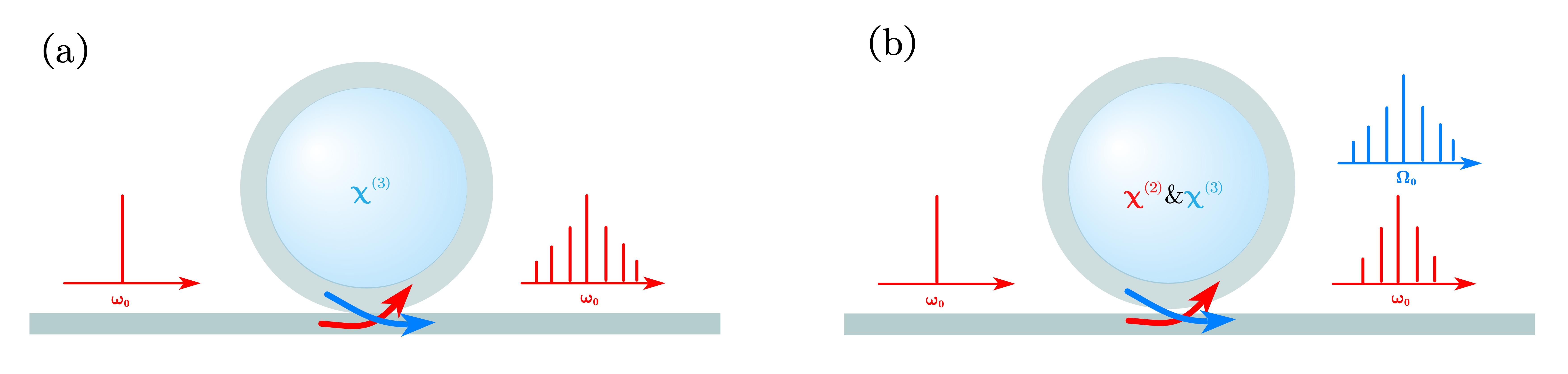
Figure 2: OFC produced by different nonlinear effects. (a) Kerr OFC. (b) Kerr micro-comb controlled by second-order nonlinear effect.

According to the literature  [9], the fluid can fully contacted with the micro-ring array, which can change the structural parameters of the micro-ring array. Different kinds and concentrations of substances will affect the structural parameters of the micro-ring tube. The direct understanding is that the change of the fluid environment inside the micro-ring cavity will lead to the change of the WGM light field on the inner wall of the tube. In order to explain that different micro-cavity structural parameters how to affect the OFC spectrum, we need to get the relationship between the OFC spectrum and the structural parameters of the micro-ring. Next, we simulate the OFC spectrum of the micro-cavity First, we model the dynamic equation of the OFC. Based on the Hamiltonian of OFC in micro-cavity, we can understand its dynamic process by creation and annihilation operators of photons.

Since only the third-order nonlinear effect is considered, we only consider one mode family: $\hat{\mathcal{H}}_{0}=\sum_{l}{\hbar\omega_{a_{l}}\hat{a}_{l}^{\dagger}\hat{a}_{l}}$, This term represents the Hamiltonian of the mode family in the micro-ring, $\hat{a}_{l}$ represents the photon annihilation operator, $\hat{a}_{l}^{\dagger}$ represents the photon creation operator, $\omega_{a_{l}}$represents the angular frequency of the corresponding photon, and $l$ represents different photons in the frequency domain. Because our micro-cavity has a high quality factor, when the pump light continuously inputs energy, the energy in the micro-cavity reaches a certain threshold, and there will be a nonlinear optical process, which is expressed as:

$$\hat{\mathcal{H}}_{\chi^{\left(3\right)}}=\sum_{klmn}{\hbar g_{klmn}\hat{a}_{k}^{\dagger}\hat{a}_{l}^{\dagger}\hat{a}_{m}\hat{a}_{n}}\,\,$$

,

$$\hbar g_{3}\approx\sqrt{\frac{\left(\hbar\omega_{1}\right)^{2}\hbar\omega_{2}\hbar\omega_{3}}{\left(\epsilon_{0}\epsilon_{2}\right)^{2}\epsilon_{1}\epsilon_{3}}}\chi^{(3)}\frac{1}{2\pi R}\frac{1}{A_{\mathrm{eff}}}\xi\,\,$$

, We only consider the third-order nonlinear effect to verify the correctness of our theory, where $g_{klmn}$ is the third-order nonlinear coefficient, representing the intensity of four-wave mixing process, $R$ is the radius of microcavity, $\xi$is the mode overlap factor on the cross section, and $0\leqslant\xi\leqslant 1$, $A_{eff}$ are the effective mode area on the cross section, and $i$is the relative dielectric constant at the frequency of $\omega_{i}$. For external pumping in p mode, we have

$$\mathcal{H}_{pump}=\hbar\epsilon_{a_{p}}\left(\hat{a}_{p}e^{i\left(\omega_{p}+\delta_{p}\right)t}+{\hat{a}_{p}}^{\dagger}e^{-i\left(\omega_{p}+\delta_{p}\right)t}\right)$$

, Where

$$\epsilon_{p}=\sqrt{\frac{kP_{in}}{\hbar\omega_{p}+\delta_{p}}}$$

is the pump field, $k=\frac{\omega_{p}}{2Q}$ represents the total coupling loss (including internal coupling and external coupling), $Q$ represents the quality factor of the resonator, and $\delta_{p}$ represents pump detuning. Similarly, in order to get rid of the dependence of the system on time, we make the system enter the rotating coordinate system with $d_{1}$as the equal interval frequency by unitary transformation matrices $\hat{U}\left(t\right)=e^{i\hat{R}t}$ and $\hat{R}=\sum_{l}{\left(\omega_{p}+d_{1}l+\delta\right)}\hat{a}_{l}^{\dagger}\hat{a}_{l}$, and get the mode family frequency: $\omega_{a}=\omega_{0}+d_{1}l+\delta$. Ignoring the higher-order dispersion, the eigenfrequency is expressed as $\omega_{j}=\omega_{0}+d_{1}l+{{d_{2}l^{2}}/{2}}$,$d_{1}$ is obtained from $FSR\cdot 2\pi$, $FSR=\frac{c}{2\pi n_{eff}R}$, $c$is the speed of light in vacuum, $n_{eff}$ is the effective refractive index of the medium, $R$ is the radius of the micro-ring, $d_{2}=-\frac{c}{n_{eff}}d_{1}^{2}\beta_{2}$, $\beta_{2}$ is the second-order group velocity dispersion, and $l$ is the interval between the expressed optical mode frequency and the center frequency $d_{1}$of the mode family, and the detuning of the mode family is expressed as $\delta_{a_{l}}=d_{2}l^{2}-\delta$respectively. Finally, the Hamiltonian of our system is obtained: $\hat{\mathcal{H}}_{sys}=\sum_{l}{\hbar\delta_{a_{l}}\hat{a}_{l}^{\dagger}\hat{a}_{l}}+\hat{\mathcal{H}}_{\chi^{\left(3\right)}}+\hbar\epsilon_{a_{0}}\left(\hat{a}_{0}+{\hat{a}_{0}}^{\dagger}\right)$ In order to linearize the system, we formally decompose the optical state into mean field solution (assuming coherent state) and quantum fluctuation: $\hat{a}_{l}\left(t\right)=\alpha_{l}\left(t\right)+\hat{a}_{l}\left(t\right)$. We only keep the second-order term in Hamiltonian and ignore the higher-order term, while removing the first-order term and constant term, and pass through Heisenberg’s equation of motion $\dot{\hat{X}}=-i\left[X,\mathcal{H}\right]-k_{x}X$, Finally, the dynamic equation of our optical frequency comb is obtained:

$$\frac{d}{dt}a_{l}=\left(-i\delta_{a_{l}}-\kappa\right)a_{l}-i\sum_{k,l,m}{2}g_{3}a_{k}^{\dagger}a_{l}a_{m}-i\epsilon_{p}\delta_{p}(l-p),$$ (1)

Where $\delta_{a_{l}}=d_{2}l^{2}-\delta$ is mode detuning and $k$ is total coupling loss.

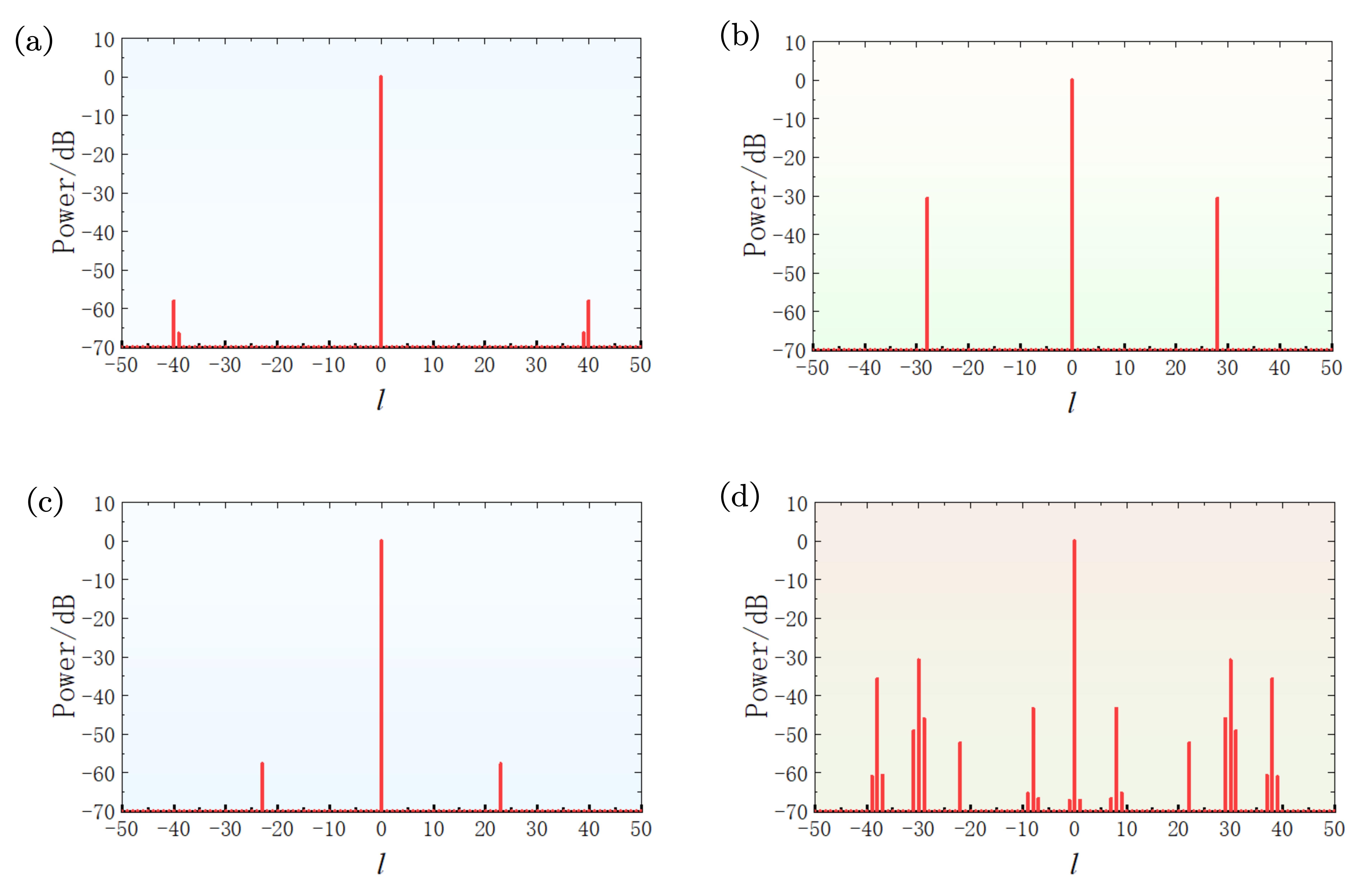
Figure 3: Influence on frequency spectrum when $d_{2}$ and $g_{3}$ take different values. The initial parameters are $d_{2}=0.004$, $k=1$, $g_{3}=1$, $\varepsilon_{p}=4.2\sqrt{2}$. (a)$d_{2}=0.003$. (b)$g_{3}=1$. (c)$d_{2}=0.005$. (b)$g_{3}=1.4$.

We use the method in [23] to change the sum term in the formula into the form of Fourier and inverse Fourier changes, and use the fourth-order Runge-Kutta numerical method to simulate the spectrum of 128 modes of optical frequency combs in the cavity. In order to facilitate the subsequent data processing, we take the normalized dimensionless parameters in [24], and the initial parameters are $d_{2}=0.004$, $k=1$, $g_{3}=1$, and $\varepsilon_{p}=4.2\sqrt{2}$. As shown in Figure 3, we can clearly see that the influence of $g_{3}$ and $d_{2}$ on the frequency spectrum is different by controlling the variables, which is consistent with the conclusion of the investigation and research on the formation position of the main comb in the literature [25]. We can see from figures 3(a) and (c) that with the increase of $d_{2}$, the lateral peak will be closer to the center of the spectrum, and it is found in literature [25] that the speed of the lateral peak approaching the central mode in the spectrum is not linear with the change of $d_{2}$. With the increase of $g_{3}$, as shown in Figures 3(b) and (d), we find that although the position of the side peak has not changed obviously in the spectrum, more comb teeth appear, which is also explained in the literature [25], which leads to micro-loops. Selecting the method of spectrum feature extraction has become an urgent problem to be solved. As shown in Figure 4, machine learning, which can independently extract data features from training data, is undoubtedly the best choice.

3 Optical information processing device and principle

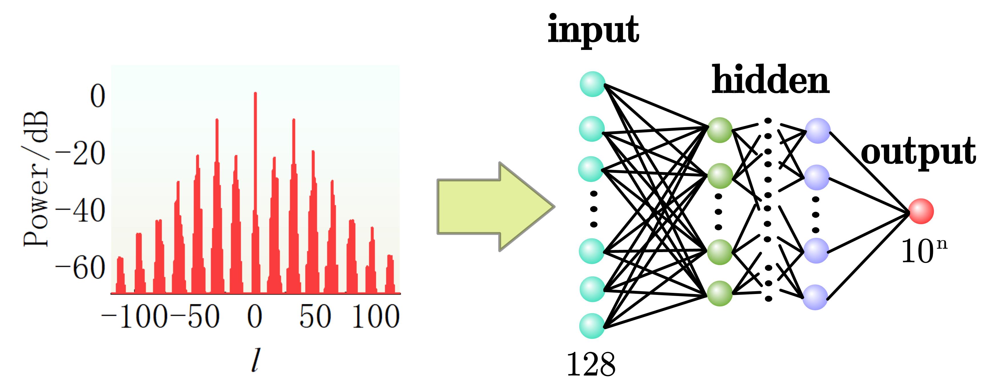
Figure 4: Simple schematic diagram of substituting optical frequency comb into neural network calculation.

To realize machine learning by optical integration, it is necessary to overcome two basic calculation processes of machine learning, one is linear activation and the other is convolution activation. The key point of the two calculations is the multiplication calculation at the real photon level. Combining with the commonly used photon detection method at present: converting optical signals into electrical signals, it is also convenient for us to analyze our sensing results in depth. We choose the light intensity as the basic measurement quantity in the photonic integrated chip. We use the coupling structure of waveguide array to realize linear activation and convolution activation respectively, as shown in Figures 5(b) and (c). Next, we analyze the concrete calculation mechanism in the waveguide array. The structure in Figure 5(a) shows the coupling structure between horizontal waveguides and vertical waveguides, which can be controlled by waveguide spacing [26] or by the melting state of liquid crystal. Here, we set up a heating device to change the coupling spacing of waveguides by controlling the temperature. Figure 5(b) shows the on-chip photon calculation process with linear activation. It has two waveguide arrays in horizontal and vertical directions. The number of horizontal waveguides corresponds to the number of optical modes in the transmission spectrum of the microcavity array, and different optical modes have different angular frequencies. We control the coupling ratio between the horizontal waveguide and the vertical waveguide to make the coupling ratio small. Roughly speaking, the light intensity in the horizontal waveguide is almost constant, and each vertical waveguide.

$$\mathrm{I}_{\mathrm{out}}=\boldsymbol{k}_{11}\boldsymbol{I}_{\boldsymbol{1}}+\boldsymbol{k}_{21}\boldsymbol{I}_{\boldsymbol{2}}+\boldsymbol{k}_{31}\boldsymbol{I}_{\boldsymbol{3}}+\boldsymbol{k}_{41}\boldsymbol{I}_{\boldsymbol{4}},$$ (2)

So as to realize the multiplication calculation on the photonic chip, the number of vertical waveguides is the number of linear neurons, and the number of linear neurons can be freely controlled by setting the number of vertical waveguides. We arrange the light modes of the output spectrum according to the way in Figure 4 c, and divide it into 16 parts, which refer to 16 light modes, as shown in Figure 5(c). A picture can be divided according to pixel points, or it can be brought into our model for calculation. Figure 5(d) shows the on-chip photon calculation process of convolution activation. The waveguide array is also composed of waveguides in horizontal and vertical directions, and each column represents the calculation of a convolution kernel. Different convolution kernel elements are set by setting the coupling ratio between each column and the horizontal waveguide. A series of optical modes on the left side of each row waveguide are combined by a wavelength division multiplexer, and the combined optical modes will perform the product operation of the same convolution kernel elements. The function of the left wavelength division multiplexer is to recombine and group the optical modes that have completed convolution operation but are combined in the same waveguide, thus presenting the results of convolution operation. It is possible to realize the calculation of the neural network on the optical chip by different combinations of 5(b) and (d).

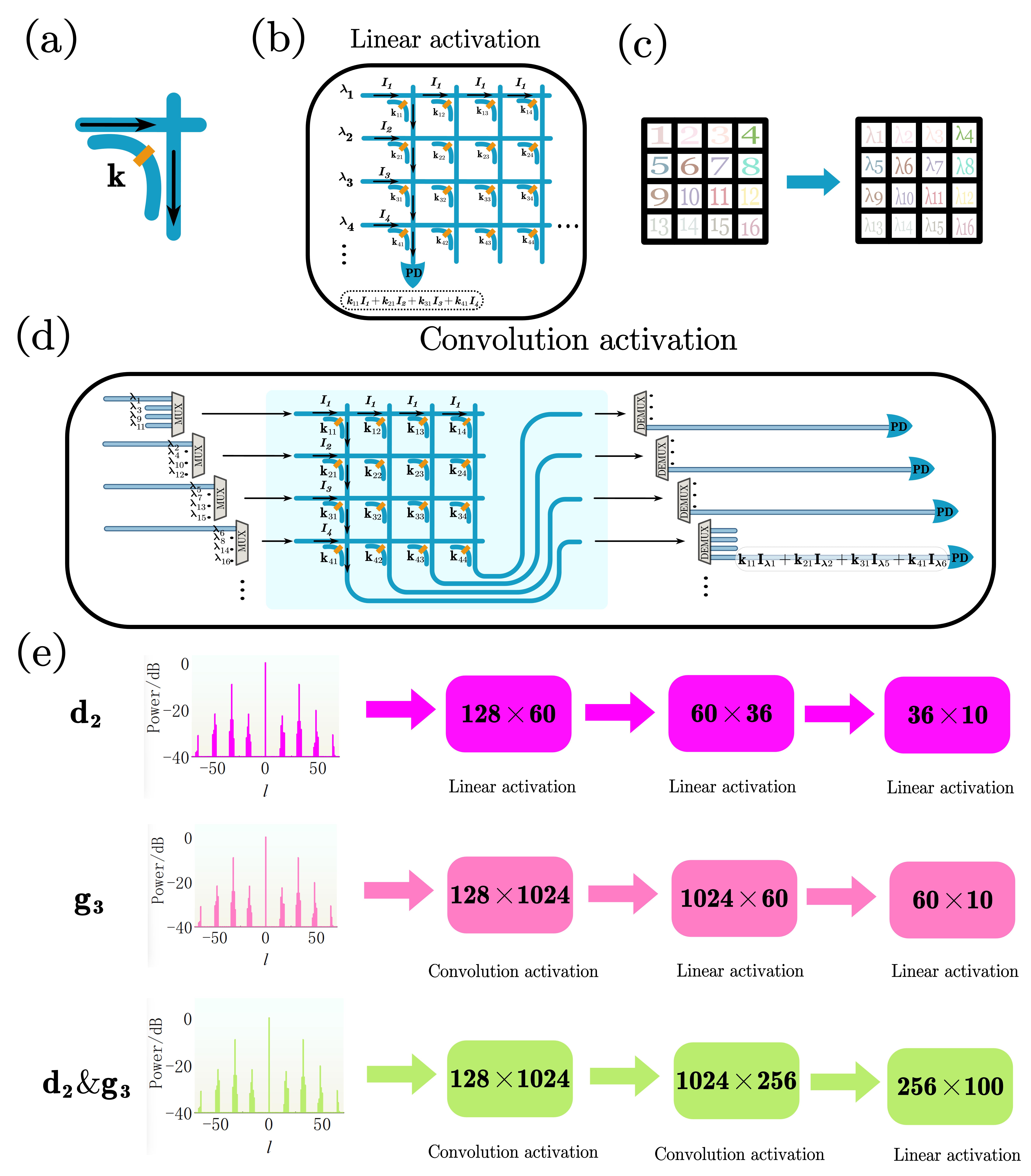
Figure 5: Integrated theoretical method for detecting fluid characteristics based on optical frequency comb technology. (a) The coupling device between the horizontal waveguide and the vertical waveguide can change the waveguide gap by changing the temperature, thus changing the coupling rate. (b) Schematic diagram of optical integrated network for linear activation. (c) The different frequencies of the input spectrum are regarded as different pixel points of a picture for convolution calculation. (d) Schematic diagram of optical integrated network for convolution activation. (d) Structure setting of neural network when different parameters are identified.

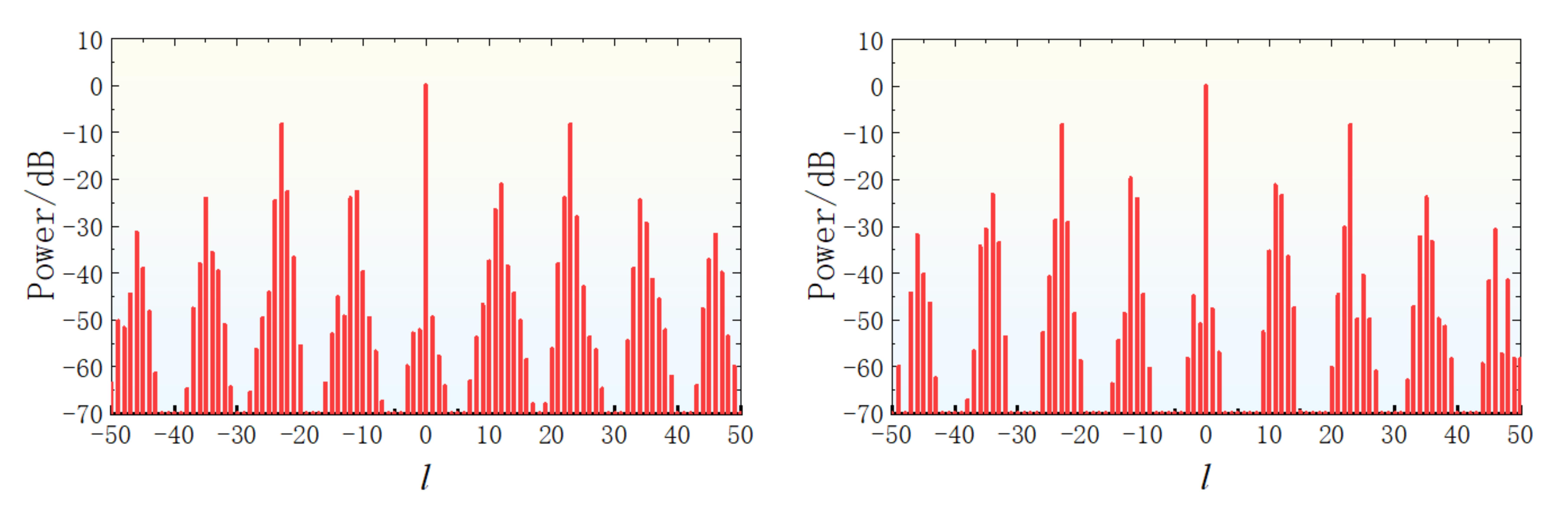
Figure 6: Spectral differences caused by different initial noises in microcavity.

4 Feasibility and accuracy analysis

In order to illustrate the feasibility and superiority of our model, the whole integration theory is simulated now. First of all, we should make it clear that machine learning is used to extract and classify the transmission spectrum characteristics of optical frequency combs in microcavity, so we need to use training data to train the neuron parameters. The training data is the intensity of each mode of the output optical frequency comb spectrum, and the comb spectrum with different characteristics is obtained through different micro-ring structure parameters. These data are input into the neural network, hoping to train a neural network that can distinguish different micro-ring structure parameters. In section 2, we know that the characteristics of transmission spectrum change with the change of micro-ring structural parameters, so we use formula (1) to simulate and get the output spectra under different micro-ring structural parameters, so as to get our training data and test data. The initial parameters are $d_{2}=0.004$, $k=1$, $g_{3}=1$, $\varepsilon_{p}=4.2\sqrt{2}$, so that the evolution of the light field in the microcavity takes the same time, and different spectra can be obtained by continuously changing the structural parameters of the micro-ring. We adjust the size of $d_{2}$ from 0.002 to 0.006, with the size interval of 0.0004, and get 10 groups of optical frequency comb spectrum data. The corresponding light intensity of each mode is represented by $\mathrm{dB}$, and these ten data are labeled as 0 to 9, thus distinguishing different $d_{2}$ and taking these ten data as one. The intensity of the initial state of the microcavity in different modes is randomly taken as a minimal complex number, as shown in Figure 6. As a result, the initial small change of the spectrum will lead to a slight difference in the spectrum, but the overall spectrum characteristics are basically similar. By increasing the number of spectrum simulations, different samples can be obtained. A similar method is also applied to the parameter $g_{3}$. By adjusting the size of $g_{3}$ from 1 to 1.5 with the size interval of 0.05, 10 groups of optical frequency comb spectrum data are obtained, and the same type of data samples are obtained by simulating the spectrum for different times.

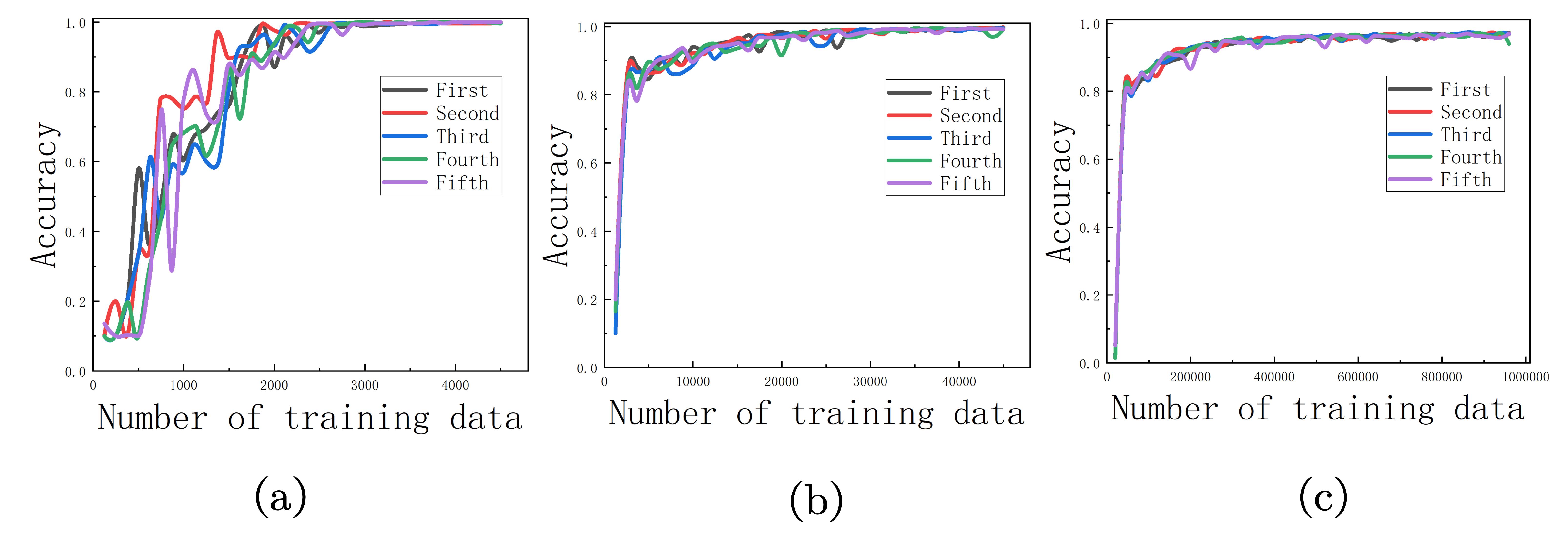
Figure 7: Visualization of the increase of recognition accuracy with the increase of data quantity under different parameter changes (five experiments have been carried out in each machine learning process). (a) The change of $d_{2}$ parameter identification accuracy with the number of training data. (b) The change of $G_{3}$ parameter identification accuracy with the number of training data. (c) The accuracy of $D_{2}$ and $g_{3}$ parameter identification varies with the number of training data.

We use the computer to train the parameters of the neural network through Pytorch. Because $d_{2}$ and $g_{3}$ have different effects on the frequency spectrum, using the neural network setup in figure 5(d), only 300 samples are needed to measure the changes of the parameters of $d_{2}$. The accuracy of 7(a) is 99.8 $\%$, and the calculation formula of accuracy is $\eta=\frac{n_{right}}{n_{exe}}$, where $n_{right}$ represents the number of correct discrimination in the test set, and $n_{exe}$ represents the test, at this time, the optimizer chosen is the algorithm of formula $\mathrm{AdaDelta}$.

$$[H]\begin{cases}E[g^{2}]_{t}=\alpha E[g^{2}]_{t-1}+(1-\alpha)g_{t}^{2}\\[8.61108pt] \Delta W_{t}=-\dfrac{\sqrt{\sum_{i=1}^{t-1}\Delta W_{i}}}{\sqrt{E[g^{2}]_{t}+\epsilon}}\\[8.61108pt] W_{t+1}=W_{t}+\Delta W_{t}\end{cases}$$ (3)

This algorithm can speed up the training, through the cross entropy loss function in the formula

$$\mathrm{Loss(}\hat{x},x)=-\sum_{i=1}^{n}{x}\log\mathrm{(}\hat{x})$$ (4)

To analyze the error between the predicted values and labels of different dimensions.

As shown in Figures 3(b) and (d), the change of $g_{3}$ leads to more complicated spectrum change. As expected, it takes more than 5000 samples to measure the change of $g_{3}$ parameters to reach Figure 7(b). And because the complexity of the spectrum increases, we change the optimizer into a more robust $\mathrm{Adam}$ algorithm, as shown in Figure 5(e), and add a convolution layer to the neural network to improve the training efficiency.

Next, we take the same parameter changes as above for the measurement under the co-variation of $d_{2}$ and $g_{3}$. Each sample now contains 100 data, and the 100 data are labeled as 0 to 99. The single digit and the ten digit respectively represent the size changes of two different parameters, and the $d_{2}$ and $g_{3}$ are traversed through different simulation times. Keeping the same neural network structure as that of $g_{3}$ recognition, the multi-layer linear layer will make the accuracy fluctuate greatly at the end. As shown in Figure 5(e), adding more convolution activation layers can improve the accuracy and stability. In order to improve the training efficiency, we increase the number of convolution kernels in convolution activation layers, and finally get the accuracy of Figure 7(c) through 10000 training samples. Through the numerical simulation of the complete integration theory, in theory, we prove that we can distinguish the spectral characteristics of multi-parameter changes by machine learning, and it has the potential to improve the recognition accuracy.

5 Conclusion

In our research, optical frequency comb, as a light source sensitive to the changes of external environment, can carry multi-dimensional fluid information through its multi-mode characteristics, thus achieving more accurate and multi-dimensional information detection and having the potential to improve sensing technology. Our work is to reveal how the projection spectrum of optical frequency comb changes by changing the structural parameters of micro-rings, and then use machine learning method to identify different transmission spectra corresponding to different fluid information. Our research does not reveal how the different substances and concentrations in the fluid affect the structural parameters of the micro-ring, but the subsequent work can find the corresponding relationship between the concentration and the structural parameters by analyzing the transmission spectra of substances with different concentrations. Moreover, because materials have excellent characteristics such as piezoelectric characteristics, magnetoelectric characteristics and thermoelectric effect, which can affect the generated optical frequency comb spectrum, our model has the potential to detect the characteristics of materials and any factors affecting the optical frequency comb spectrum. In a word, our work proves that it is feasible in theory to realize on-chip fluid information detection by using the light source of micro-cavity optical frequency comb, and it can ensure sufficient accuracy.

[H] Identified parameter 4000 4125 4250 4375 4500 $d_{2}$ 1 0.996 0.998 0.998 1 $d_{2}$ 0.996 0.996 0.998 0.998 1 $d_{2}$ 1 0.998 1 1 1 $d_{2}$ 1 1 1 0.998 0.996 $d_{2}$ 1 1 1 1 1

Table 1: The change of $d_{2}$ recognition accuracy with the amount of data.

Table 2: The change of $g_{3}$ recognition accuracy with the amount of data.

Identified parameter	40000	41250	42500	43750	45000
$g_{3}$	0.98637	0.99619	0.99519	0.99559	0.99659
$g_{3}$	0.99238	0.99359	0.99599	0.99499	0.9982
$g_{3}$	0.99319	0.99098	0.99399	0.99639	0.99499
$g_{3}$	0.99279	0.99539	0.99198	0.96954	0.99279
$g_{3}$	0.99158	0.99499	0.99218	0.99319	0.99218

Table 3: The accuracy of $d_{2}$ and $g_{3}$ parameter identification varies with the amount of data.

Identified parameter	880000	900000	920000	940000	960000
$d_{2}$ and $g_{3}$	0.96828	0.95862	0.9679	0.96862	0.97194
$d_{2}$ and $g_{3}$	0.96932	0.96664	0.97272	0.9654	0.9675
$d_{2}$ and $g_{3}$	0.97166	0.96732	0.96552	0.97168	0.96836
$d_{2}$ and $g_{3}$	0.97036	0.96864	0.96096	0.97118	0.93958
$d_{2}$ and $g_{3}$	0.9632	0.96172	0.95812	0.95684	0.96976

References

- [1] X. Jiang, A. J. Qavi, S. H. Huang, and L. Yang, “Whispering-gallery sensors,” Matter, vol. 3, no. 2, pp. 371–392, 2020.
- [2] T. Xue, W. Liang, Y. Li, Y. Sun, Y. Xiang, Y. Zhang, Z. Dai, Y. Duo, L. Wu, K. Qi et al., “Ultrasensitive detection of mirna with an antimonene-based surface plasmon resonance sensor,” Nature communications, vol. 10, no. 1, p. 28, 2019.
- [3] S. C. D. Kuhnline et al., “Interfacing lipid bilayer nanodiscs and silicon photonic sensor arrays for multiplexed protein–lipid and protein–membrane protein interaction screening,” 2013.
- [4] Q. Chen, L. Chen, Z. Fu, S. Xie, Q. Lu, and X. Zhang, “Optical frequency comb-based aerostatic micro pressure sensor aided by machine learning,” IEEE Sensors Journal, 2023.
- [5] J. H. Wade, A. T. Alsop, N. R. Vertin, H. Yang, M. D. Johnson, and R. C. Bailey, “Rapid, multiplexed phosphoprotein profiling using silicon photonic sensor arrays,” ACS Central Science, vol. 1, no. 7, pp. 374–382, 2015.
- [6] J. H. Wade and R. C. Bailey, “Applications of optical microcavity resonators in analytical chemistry,” Annual Review of Analytical Chemistry, vol. 9, pp. 1–25, 2016.
- [7] Y. Sun and X. Fan, “Optical ring resonators for biochemical and chemical sensing,” Analytical and bioanalytical chemistry, vol. 399, pp. 205–211, 2011.
- [8] J. T. Gohring, P. S. Dale, and X. Fan, “Detection of her2 breast cancer biomarker using the opto-fluidic ring resonator biosensor,” Sensors and Actuators B: Chemical, vol. 146, no. 1, pp. 226–230, 2010.
- [9] Z. Li, H. Zhang, B. T. T. Nguyen, S. Luo, P. Y. Liu, J. Zou, Y. Shi, H. Cai, Z. Yang, Y. Jin et al., “Smart ring resonator–based sensor for multicomponent chemical analysis via machine learning,” Photonics Research, vol. 9, no. 2, pp. B38–B44, 2021.
- [10] A. Nath, W. M. Atkins, and S. G. Sligar, “Applications of phospholipid bilayer nanodiscs in the study of membranes and membrane proteins,” Biochemistry, vol. 46, no. 8, pp. 2059–2069, 2007.
- [11] I. Toumi, S. Caldarelli, and B. Torrésani, “A review of blind source separation in nmr spectroscopy,” Progress in nuclear magnetic resonance spectroscopy, vol. 81, pp. 37–64, 2014.
- [12] R. Wehrens and B.-H. Mevik, “The pls package: principal component and partial least squares regression in r,” 2007.
- [13] Y. Roggo, P. Chalus, L. Maurer, C. Lema-Martinez, A. Edmond, and N. Jent, “A review of near infrared spectroscopy and chemometrics in pharmaceutical technologies,” Journal of pharmaceutical and biomedical analysis, vol. 44, no. 3, pp. 683–700, 2007.
- [14] Y. LeCun, Y. Bengio, and G. Hinton, “Deep learning,” nature, vol. 521, no. 7553, pp. 436–444, 2015.
- [15] J. Schmidhuber, “Deep learning in neural networks: An overview,” Neural networks, vol. 61, pp. 85–117, 2015.
- [16] H. M. Robison, P. Escalante, E. Valera, C. L. Erskine, L. Auvil, H. C. Sasieta, C. Bushell, M. Welge, and R. C. Bailey, “Precision immunoprofiling to reveal diagnostic signatures for latent tuberculosis infection and reactivation risk stratification,” Integrative Biology, vol. 11, no. 1, pp. 16–25, 2019.
- [17] J. Vamathevan, D. Clark, P. Czodrowski, I. Dunham, E. Ferran, G. Lee, B. Li, A. Madabhushi, P. Shah, M. Spitzer et al., “Applications of machine learning in drug discovery and development,” Nature reviews Drug discovery, vol. 18, no. 6, pp. 463–477, 2019.
- [18] F. Cheng and Z. Zhao, “Machine learning-based prediction of drug–drug interactions by integrating drug phenotypic, therapeutic, chemical, and genomic properties,” Journal of the American Medical Informatics Association, vol. 21, no. e2, pp. e278–e286, 2014.
- [19] A. Moraru, M. Pesko, M. Porcius, C. Fortuna, and D. Mladenic, “Using machine learning on sensor data,” Journal of computing and information technology, vol. 18, no. 4, pp. 341–347, 2010.
- [20] W. Zhao, A. Bhushan, A. D. Santamaria, M. G. Simon, and C. E. Davis, “Machine learning: A crucial tool for sensor design,” Algorithms, vol. 1, no. 2, pp. 130–152, 2008.
- [21] X. Guo, C.-L. Zou, and H. X. Tang, “Second-harmonic generation in aluminum nitride microrings with 2500%/w conversion efficiency,” Optica, vol. 3, no. 10, pp. 1126–1131, 2016.
- [22] A. W. Bruch, X. Liu, Z. Gong, J. B. Surya, M. Li, C.-L. Zou, and H. X. Tang, “Pockels soliton microcomb,” Nature Photonics, vol. 15, no. 1, pp. 21–27, 2021.
- [23] T. Hansson, D. Modotto, and S. Wabnitz, “On the numerical simulation of kerr frequency combs using coupled mode equations,” Optics Communications, vol. 312, pp. 134–136, 2014.
- [24] Y. K. Chembo and N. Yu, “Modal expansion approach to optical-frequency-comb generation with monolithic whispering-gallery-mode resonators,” Physical Review A, vol. 82, no. 3, p. 033801, 2010.
- [25] H. Shen and C. Zhao, “A method for determining the formation position of comb tooth of kerr micro-ring,” IEEE Journal of Quantum Electronics, 2023.
- [26] X. Guo, C.-L. Zou, and H. X. Tang, “70 db long-pass filter on a nanophotonic chip,” Optics express, vol. 24, no. 18, pp. 21 167–21 176, 2016.