Convergence Analysis of Probability Flow ODE for Score-based Generative Models

Abstract.

Score-based generative models have emerged as a powerful approach for sampling high-dimensional probability distributions. Despite their effectiveness, their theoretical underpinnings remain relatively underdeveloped. In this work, we study the convergence properties of deterministic samplers based on probability flow ODEs from both theoretical and numerical perspectives. Assuming access to $L^{2}$-accurate estimates of the score function, we prove the total variation between the target and the generated data distributions can be bounded above by $\mathcal{O}(d\sqrt{\delta})$ in the continuous time level, where $d$ denotes the data dimension and $\delta$ represents the $L^{2}$-score matching error. For practical implementations using a $p$-th order Runge-Kutta integrator with step size $h$, we establish error bounds of $\mathcal{O}(d(\sqrt{\delta}+(dh)^{p}))$ at the discrete level. Finally, we present numerical studies on problems up to $128$ dimensions to verify our theory, which indicate a better score matching error and dimension dependence.

1. Introduction

In recent years, score-based generative models [35, 18, 37, 38, 13] have emerged as a powerful paradigm for sampling high-dimensional probability distributions. Unlike traditional generative models that directly parameterize the mapping from random noise to target distribution samples [20, 17, 33, 30], score-based generative models consist of two stochastic processes—the forward and reverse processes. The forward process transforms samples from the target data distribution $\mu_{\ast}$ with density $q_{0}$ into pure noise, a step commonly referred to as the diffusion process. The gradient of the log-density function, also known as the score function, is learned from these trajectories using score matching techniques [19, 42, 37, 38]. The reverse process, guided by the score function, transforms random noise back into samples from $q_{0}$. This methodology has been proven effective in synthesizing high-fidelity audio and image data [12, 13, 31, 32, 14].

The reverse process is commonly implemented either as stochastic dynamics or deterministic dynamics, the latter often formulated as probability flow ordinary differential equation (ODE). These probability flow ODEs can typically be discretized using numerical methods such as forward Euler, exponential integrator, Heun, and high-order Runge-Kutta methods. Recent advancements in methods like those proposed in [36, 38, 28, 29, 44, 45] have enabled denoising steps to be completed in just a few iterations (e.g., 50 steps), compared to the Euler-Maruyama scheme typically employed for stochastic dynamics, which often requires a significantly larger number of steps (e.g., 1000 steps). Consequently, these deterministic methods achieve better efficiency in generating samples with only moderate quality degradation. The deterministic dynamics depends on the score function, which is typically learned by a neural network through the score matching process involving non-convex optimization. Consequently, the score estimation is inherently imperfect. This imprecision, coupled with discretization error, poses a critical question: How does the interplay between score matching error and discretization error influence the convergence of the deterministic dynamics towards the true data distribution? Our work seeks to address this question by delving into the convergence analysis of probability flow ODEs within the context of score-based generative models.

For the stochastic dynamics, convergence analyses have been explored in various works such as [5, 11, 43, 21, 39, 22, 9, 23, 7, 40], with notable contributions from [9, 23, 7, 40], offering convergence guarantees with polynomial complexity, without relying on any structural assumptions on the data distribution like log-concavity. The stochastic nature of these dynamics plays a crucial role in mitigating error accumulation. However, the deterministic counterpart warrants further exploration. Related works include [10], which assumes no score matching error and provides a discretization analysis for the probability flow ODE in KL divergence. However, their bounds exhibit a large dependence on dimensionality and are exponential in the Lipschitz constant of the score integrated over time. In contrast, [8] assumes $L^{2}$ bounds on the score estimation offers polynomial-time convergence guarantees for the probability flow ODE combined with a stochastic Langevin corrector, without relying on any structural assumptions on the data distribution. Similarly, [24, 25] provide polynomial-time convergence guarantees for the probability flow ODE by requiring control of the difference between the derivatives of the true and approximate scores. Additionally, [2, 4] analyze the convergence of the deterministic dynamics at continuous time level, exhibiting exponential dependence on the Lipschitz constant, stemming from a more general stochastic interpolant or flow matching setup [26, 27, 1, 6]. Finally, [16] offers convergence analysis for the general probability flow ODEs with log-concavity data assumption, where the error bounds grow exponentially with time $T$ in the presence of the score matching error.

1.1. Our Contributions

We analyze the convergence of the probability flow ODE from both theoretical and numerical perspectives. Our detailed contributions are as follows:

• We provide convergence guarantees of the probability flow ODE at the continuous time level under three mild assumptions. These assumptions are as follows: 3.1 asserts that the target density has a compact support, 3.2 asserts the $L^{2}$ score matching error over time is bounded by $\delta$, and 3.3 asserts the first and second derivatives of the estimated score are bounded. Under these assumptions, we prove in Theorem 3.4 that the total variation distance between the target and the generated data distributions can be bounded above by $\mathcal{O}(d\sqrt{\delta})$, where $d$ is the data dimension.

• We provide convergence guarantees of the probability flow ODE at the disretized level. To accommodate a $p$-th order time integrator, we further require 3.7, that the estimated score function’s first $(p+1)$-th derivatives are bounded. We establish in Theorem 3.9 that the total variation distance between the target and the generated data distributions can be bounded above by $\mathcal{O}(d(\sqrt{\delta}+(dh)^{p}))$ .

• We verify our theoretical discoveries through numerical studies on problems with Gaussian mixture target densities up to 128 dimensions. By intentionally introducing artificial score matching errors and employing the widely used second-order Heun’s time integrator, our numerical results demonstrate a total variation error of $\mathcal{O}(\delta+h^{2})$ (for the marginal distributions), with improved dependencies on dimension and score matching error.

In our theoretical proof at the continuous time level, we combine the method of characteristic lines and calculus of variations to estimate the total variation between the generated data distribution $\widehat{q}_{t}$ and the target distribution $q_{t}$ along the diffusion process. Compared to using Grönwall’s inequality directly, our error estimate in Theorem A.1 does not include an exponential term in time. We provide two mathematically rigorous yet simple proofs of Theorem A.1, and also illustrate our intuition in Section A. Furthermore, our methods imply a more general Theorem A.3 for the $L^{1}$-norms of solutions of general transport equations. In Remark 3.10 and Remark A.4, we highlight that our methods can also estimate the $L^{1}(\mathbb{R}^{d})$-norms of derivatives of $\widehat{q}_{t}-q_{t}$. Consequently, we can conclude that the $L^{r}(\mathbb{R}^{d})$-norm of $\widehat{q}_{t}-q_{t}$ is also small when $r>1$. See Remark 3.10 and Remark A.4 for further details. Additionally, our method extends to estimating the pointwise difference between $\widehat{q}_{t}$ and $q_{t}$, although we defer this investigation to future work to maintain the manuscript’s conciseness. In our proof of Theorem 3.4, we leverage the Gagliardo-Nirenberg interpolation inequality with a universal constant, meaning the constant is independent of the dimension. To provide a comprehensive literature review, we include the proof of this dimension-free interpolation inequality as Lemma C.1.

For our convergence analysis of the probability ODE flow at the discretized level, a first step is to reformulate the discrete solution obtained by the $p$-th order Runge-Kutta method as a continuous-time ODE flow using interpolation. We derive an interpolation in Proposition D.1, and crucially, the score function associated with the interpolated ODE flow and the original approximated score function (and their derivatives) are close up to a $p$-th order error, i.e., $\mathcal{O}(h^{p})$. Employing the characteristic method described in Appendix A again, the error at the discrete level decomposes into two parts: the score matching error between the generated data distribution $\widehat{q}_{t}$ and the target distribution $q_{t}$ along the diffusion process, and the discretization error between the interpolated ODE flow solution and the generated data distribution $\widehat{q}_{t}$. Consequently, the score matching error and time discretization error do not interact to magnify, thus preserving the time discretization error at the $p$-th order.

Our assumptions on the true data distribution $\mu_{\ast}$ are quite general. In 3.1, we assume that $\mu_{\ast}$ has a compact support. In Appendix B, we extend our main result to the case where $\mu_{\ast}$ is a Gaussian mixture. We emphasize that under 3.1, $\mu_{\ast}$ may not have a density, and the compact support $K_{\ast}$ of $\mu_{\ast}$ can be a submanifold of a much lower dimension in $\mathbb{R}^{d}$, particularly point masses. Refer to our Example B.1 and Example B.2, where we observe that assuming $\nabla\log q_{t}$ is uniformly Lipschitz with a constant independent of $t$ is unreasonable, as it actually tends to $\infty$ as $t\to 0^{+}$. In Lemma B.3 and Lemma B.5, we compute and estimate the high-order derivatives of $q_{t}$ (and $\log q_{t}$), when $\mu_{\ast}$ has a compact support and when $\mu_{\ast}$ is a Gaussian mixture. For Gaussian mixtures, the error estimates are better than the case when $K_{\ast}$ is a submanifold of a much lower dimension. We also mention in Remark C.4 that our methods also apply to other reasonable assumptions on $\mu_{\ast}$ once some simple estimates are satisfied.

1.2. Natations

• Diacritics: $\widehat{\square}$ denotes quantities involve score error, $\widetilde{\square}$ denotes quantities involve time discretization error.

• Time steps: $0=t_{0}<t_{1}<\cdots<t_{N}=T-\tau$, where $\tau>0$ is a small parameter.

• Distributions on $\mathbb{R}^{d}$: $q_{t},\widehat{q}_{t},\widetilde{q}_{t}$ denote forward process, $\varrho_{t}=q_{T-t},\widehat{\varrho}_{t}=\widehat{q}_{T-t},\widetilde{\varrho}_{t}=\widetilde{q}_{T-t}$ reverse process. We also define $\widehat{\varepsilon}_{t}(x)\coloneq\widehat{q}_{t}(x)-q_{t}(x),\widetilde{\varepsilon}_{t}(x)\coloneq\widetilde{q}_{t}(x)-q_{t}(x)$.

• Vector fields from $\mathbb{R}^{d}$ to $\mathbb{R}^{d}$: Forward process: $U_{t}(x)\coloneq x+\nabla\log q_{t}(x)$, $\widehat{U}_{t}\coloneq x+s_{T-t}(x)$, $\widetilde{U}_{t}\coloneq x+\widetilde{s}_{T-t}(x)$, $\delta_{t}(x)\coloneq\widehat{U}_{t}-U_{t}=s_{T-t}(x)-\nabla\log q_{t}(x)$, $\widetilde{\delta}_{t}(x)\coloneq\widetilde{U}_{t}(x)-U_{t}(x)$; Reversal process: $V_{t}\coloneq U_{T-t}$, $\widehat{V}_{t}\coloneq\widehat{U}_{T-t}$, $\widetilde{V}_{t}\coloneq\widetilde{U}_{T-t}$; Other vector fields: $Z_{t}(x)$.

• $\alpha=(\alpha_{1},\alpha_{2},\ldots,\alpha_{d})$ is a multi-index with nonnegative integers $\alpha_{i}$’s, $|\alpha|\coloneq\alpha_{1}+\alpha_{2}+\ldots+\alpha_{d}$, and we define $\partial_{x}^{\alpha}\coloneq\partial_{x_{1}}^{\alpha_{1}}\partial_{x_{2}}^{\alpha_{2}}\cdots\partial_{x_{d}}^{\alpha_{d}}$. We also use $\partial_{i}\coloneq\partial_{x_{i}}$ for simplicity.

• Constants: We use $C_{u}$ to denote universal constants like $10,50,100,200$, i.e., $C_{u}$ is independent of the dimension $d$ and other parameters in this paper. Also, $C_{u}$ may vary by lines.

• Norms: For a vector $x=(x_{1},x_{2},\ldots,x_{d})\in\mathbb{R}^{d}$, we use $\|x\|=\|x\|_{2}\coloneq{(x_{1}^{2}+x_{2}^{2}+\ldots+x_{d}^{2})}^{\frac{1}{2}}$, $\|x\|_{\infty}\coloneq\sup_{1\leq i\leq d}|x_{i}|$, $\|x\|_{1}\coloneq|x_{1}|+|x_{2}|+\ldots+|x_{d}|$, $\|x\|_{p}\coloneq{({|x_{1}|}^{p}+{|x_{2}|}^{p}+\ldots+{|x_{d}|}^{p})}^{\frac{1}{p}}$. We similarly define $\|\cdot\|_{2}$, $\|\cdot\|_{\infty}$, $\|\cdot\|_{1}$, $\|\cdot\|_{p}$, for matrices or even more general tensors, because we can view them as vectors and forget their tensor structures. For a vector-valued function $F(x)=(f_{1}(x),f_{2}(x),\ldots,f_{m}(x)):\mathbb{R}^{d}\mapsto\mathbb{R}^{m}$, where $m$ is a positive integer, we usually regard $F(x)$ as a vector in $\mathbb{R}^{m}$ and similarly use the notations $\|F(x)\|$, $\|F(x)\|_{1}$, $\|F(x)\|_{\infty}$.

• Function class: We say a vector-valued function $F(x)=(f_{1}(x),f_{2}(x),\ldots,f_{m}(x)):{\mathbb{R}}^{d}\mapsto{\mathbb{R}}^{m}$ as being in $C^{r}$, if each of its components $f_{i}(x)$ has continuous first $r$-th derivatives. We say $F(x)$ is in the $L^{s}$-space $L^{s}(\mathbb{R}^{d})$ if for each of its components $f_{i}(x)$, its $L^{s}(\mathbb{R}^{d})$-norm defined as $\|f_{i}\|_{L^{s}(\mathbb{R}^{d})}\coloneq{(\int_{\mathbb{R}^{d}}{|f_{i}(x)|}^{s}{\rm d}x)}^{\frac{1}{s}}$ is finite. We say $F(x)$ is in the Sobolev space $W^{r,s}(\mathbb{R}^{d})$ if for each of its components $f_{i}(x)$, $\partial_{x}^{\alpha}f_{i}\in L^{s}(\mathbb{R}^{d})$ for each $\alpha$ with $|\alpha|\leq r$. We define the $W^{r,s}(\mathbb{R}^{d})$-norm of $f_{i}$ as $\|f_{i}\|_{W^{r,s}(\mathbb{R}^{d})}\coloneq(\sum_{|\alpha|\leq r}\|\partial_{x}^{\alpha}f_{i}\|_{L^{s}(\mathbb{R}^{d})}^{s})^{\frac{1}{s}}$.

2. Preliminaries

2.1. Score-based Generative Model

Score-based generative models begin with $d$ dimensional true data samples $\{X_{0}\}$ following an unknown target distribution $\mu_{\ast}$ with density $q_{0}$. The objective is to sample new data from the target distribution. Typically, the score-based generative models usually involve two processes—the forward and reverse processes.

In the forward process, we start with data samples from $q_{0}$, and progressively transform the data into noise. This process is often based on the canonical Ornstein-Uhlenbeck (OU) process given by

(1) $${\rm d}X_{t}=-X_{t}{\rm d}t+\sqrt{2}{\rm d}B_{t},\qquad X_{0}\sim q_{0},\qquad 0\leq t\leq T,$$

where $(B_{t})_{t\in[0,T]}$ is a standard Brownian motion in $\mathbb{R}^{d}$. The OU process has an analytical solution

(2) $$X_{t}\overset{d}{=}\lambda_{t}X_{0}+\sigma_{t}W,\qquad W\sim{\mathcal{N}}(0,{\mathbb{I}}_{d}),$$

with $\lambda_{t}=e^{-t}$ and $\sigma_{t}=\sqrt{1-e^{-2t}}$. The OU process exponentially converges to its stationary distribution, the standard Gaussian distribution ${\mathcal{N}}(0,{\mathbb{I}}_{d})$. Let $q_{t}$ denote the density of $X_{t}$, which evolves according to the following Fokker–Planck equation:

$$\partial_{t}q_{t}=\nabla\cdot\bigl{(}(x+\nabla\log q_{t}(x))q_{t}\bigr{)}=\nabla\cdot(U_{t}q_{t}),\qquad 0\leq t\leq T,$$

with $U_{t}(x)\coloneq x+\nabla\log q_{t}(x)$.

By denoting $\varrho_{t}=q_{T-t}$, the time reversal process from time $T$ to $0$, satisfies the following partial differential equation (PDE):

(3) $$\begin{split}\partial_{t}\varrho_{t}=-\nabla\cdot\bigl{(}(x+\nabla\log q_{T-t})\varrho_{t}\bigr{)}=-\nabla\cdot(V_{t}\varrho_{t}),\qquad 0\leq t\leq T,\end{split}$$

with $V_{t}(x)\coloneq x+\nabla\log q_{T-t}(x)$. The score function $\nabla\log q_{T-t}(x)$ is typically learned by a neural network trained using score matching techniques with progressively corrupted trajectories $\{X_{t}\}$ from (1). Subsequently, the reverse PDE can be solved from $\varrho_{0}=q_{T}$ to sample new data from $q_{0}$.

The reverse PDE (3) is often reformulated into a mean field equation for sampling instead of being directly solved. This mean field equation can manifest as stochastic dynamics

(4) $${\rm d}Y_{t}=\left(Y_{t}+2\nabla\log q_{T-t}(Y_{t})\right){\rm d}t+\sqrt{2}{\rm d}B_{t}^{\prime},\qquad Y_{0}\sim q_{T},\qquad 0\leq t\leq T,$$

where $(B_{t}^{\prime})_{0\leq t\leq T}$ is a Brownian motion in $\mathbb{R}^{d}$. This formulation is commonly referred to as the denoising diffusion probabilistic model (DDPM). Alternatively, the mean-field equation can adopt a deterministic dynamics framework in terms of an ordinary differential equation with velocity field $V_{t}$:

(5) $$\partial_{t}Y_{t}=Y_{t}+\nabla\log q_{T-t}(Y_{t})=V_{t}(Y_{t}),\qquad Y_{0}\sim q_{T},\qquad 0\leq t\leq T,$$

known as the probability flow ODE. Additionally, when $\nabla\log q_{T-t}(x)$, is represented by the learned score function $s_{t}(x)$, the probability flow ODE (5) becomes

(6) $$\partial_{t}\widehat{Y}_{t}=\widehat{Y}_{t}+s_{t}(\widehat{Y}_{t})=\widehat{V}_{t}(\widehat{Y}_{t}),\qquad\widehat{Y}_{0}\sim\widehat{\varrho}_{0},$$

here the velocity field becomes $\widehat{V}_{t}(x)\coloneq x+s_{t}(x)$. And $\widehat{Y}_{0}$ is sampled from $\widehat{\varrho}_{0}$, since the density $q_{T}$ is unknown. $\widehat{\varrho}_{0}$ is commonly approximated by the standard Gaussian distribution ${\mathcal{N}}(0,{\mathbb{I}}_{d})$, which serves as a reliable approximation of $q_{T}$ for sufficiently large $T$. The associated density of $\widehat{Y}_{t}$ is denoted as $\widehat{\varrho}_{t}$, which differs from $\varrho_{t}$ that describes the density of $Y_{t}$, due to the score matching error.

2.2. Time Integrator

To numerically solve the probability flow ODE (6), a time integrator is essential. Fix a small $\tau>0$, we discretize the time interval $[0,\,T-\tau]$ into $N$ time steps $0=t_{0}<t_{1}<\cdots<t_{N}=T-\tau$, typically using a uniform step size $h=(T-\tau)/{N}$, Starting from an initial condition $\widetilde{Y}_{t_{0}}$ sampled from $q_{T}$, the time integrator iteratively estimates $\widetilde{Y}_{t_{i}}$ at time $t_{i}$. One commonly used time integrator is the Runge-Kutta method, the family of explicit $s$-stage $p$-th order Runge-Kutta methods updates $\{\widetilde{Y}_{t_{i}}\}$ as follows:

(7) $$\widetilde{Y}_{t_{i+1}}=\widetilde{Y}_{t_{i}}+h\sum_{j=1}^{s}b_{j}k_{j},$$

where

(8) $$\begin{split}&k_{1}=\widehat{V}_{t_{i}+c_{1}h}\bigl{(}\widetilde{Y}_{t_{i}}\bigr{)},\\ &k_{2}=\widehat{V}_{t_{i}+c_{2}h}\bigl{(}\widetilde{Y}_{t_{i}}+(a_{21}k_{1})h\bigr{)},\\ &k_{3}=\widehat{V}_{t_{i}+c_{3}h}\bigl{(}\widetilde{Y}_{t_{i}}+(a_{31}k_{1}+a_{32}k_{2})h\bigr{)},\\ &\qquad\qquad\qquad\vdots\\ &k_{s}=\widehat{V}_{t_{i}+c_{s}h}\bigl{(}\widetilde{Y}_{t_{i}}+(a_{s1}k_{1}+a_{s2}k_{2}+\cdots+a_{s,s-1}k_{s-1})h\bigr{)}.\end{split}$$

The lower triangular matrix $[a_{jk}]$ is called the Runge–Kutta matrix, while the $b_{j}$ and $c_{j}$ are known as the weights and the nodes. The stage number $s$ and the parameters are chosen such that the local truncation error of (7) is $\mathcal{O}(h^{p+1})$. In general, $s\geq p$ and if $p\geq 5$, then $s\geq p+1$.

For example, forward Euler scheme is the 1-stage first order Runge-Kutta method:

$$\widetilde{Y}_{t_{i+1}}=\widetilde{Y}_{t_{i}}+hk_{1}\qquad k_{1}=\widehat{V}_{t_{i}}\bigl{(}\widetilde{Y}_{t_{i}}\bigr{)}$$

Heun’s method is the 2-stage second order Runge-Kutta method:

$$\widetilde{Y}_{t_{i+1}}=\widetilde{Y}_{t_{i}}+\frac{h}{2}(k_{1}+k_{2})\qquad k_{1}=\widehat{V}_{t_{i}}\bigl{(}\widetilde{Y}_{t_{i}}\bigr{)}\qquad k_{2}=\widehat{V}_{t_{i+1}}\bigl{(}\widetilde{Y}_{t_{i}}+hk_{1}\bigr{)}$$

Remark 2.1.

The time discretization error between Runge-Kutta solution $\widetilde{Y}_{t_{i}}$ and the true solution $\widehat{Y}_{t_{i}}$ is typically analyzed through the concept of local truncation error, which is interpreted as follows. Consider any time interval $[t_{i},t_{i+1}]$, solve (6) in the time interval with $\widetilde{Y}_{t_{i}}=\widehat{Y}_{t_{i}}$ analytically, gives

(9) $$\widehat{Y}_{t_{i+1}}=\widetilde{Y}_{t_{i}}+h\widehat{V}_{t_{i}}(\widetilde{Y}_{t_{i}})+\frac{h^{2}}{2}\frac{{\rm d}\widehat{V}_{t_{i}}(\widetilde{Y}_{t_{i}})}{{\rm d}t}+\cdots+\frac{h^{p}}{p!}\frac{{\rm d}^{p-1}\widehat{V}_{t_{i}}(\widetilde{Y}_{t_{i}})}{{\rm d}t^{p-1}}+\frac{1}{(p+1)!}\int_{t_{i}}^{t_{i+1}}(t_{i+1}-t)^{p}\frac{{\rm d}^{p}\widehat{V}_{t}(\widetilde{Y}_{t})}{{\rm d}t^{p}}{\rm d}t.$$

Similarly for the $s$-stage $p$-th order Runge-Kutta methods (7), we can view $\widetilde{Y}_{t_{i}+r}=\widetilde{F}_{r}(\widetilde{Y}_{t_{i}})$ as a function of $r\in[0,h]$ (by replacing $h$ to $r$ in (7) amd (8)) and $\widetilde{Y}_{t_{i}}$, and perform a Taylor expansion around $r=0$

(10) $$\widetilde{Y}_{t_{i+1}}=\widetilde{Y}_{t_{i}}+h\frac{{\rm d}F_{0}(\widetilde{Y}_{t_{i}})}{{\rm d}r}+\cdots+\frac{h^{p}}{p!}\frac{{\rm d}^{p}F_{0}(\widetilde{Y}_{t_{i}})}{{\rm d}r^{p}}+\frac{1}{(p+1)!}\int_{0}^{t_{i+1}-t_{i}}(h-r)^{p}\frac{{\rm d}^{p+1}\widetilde{F}_{r}(\widetilde{Y}_{t_{i}})}{{\rm d}r^{p+1}}{\rm d}r.$$

The Runge–Kutta matrix $[a_{jk}]$, weights $b_{j}$ and nodes $c_{j}$ are carefully chosen such that the coefficients in front of $h,h^{2},\cdots,h^{p}$ (as a function of $\widetilde{Y}_{t_{i}}$) in (9) and (10) cancel perfectly. Thus the Runge-Kutta estimation $\widetilde{Y}_{t_{i+1}}$ satisfies

$$\widetilde{Y}_{t_{i+1}}=\widehat{Y}_{t_{i+1}}+R_{p+1}(\widehat{V}_{t},\widetilde{Y}_{i},t_{i},h),\quad R_{p+1}(\widehat{V}_{t},\widetilde{Y}_{t_{i}},t_{i},h)=\mathcal{O}(h^{p+1}).$$

3. Main Results

The probability flow ODE (5) describes the evolution of $Y_{t}$; while its counterpart with the estimated score function (6) describes the evolution of $\widehat{Y}_{t}$. We denote the density of $Y_{t}$ and $\widehat{Y}_{t}$ as $\varrho_{t}$ and $\widehat{\varrho}_{t}$ respectively. Then they satisfy the following PDEs

(11) $$\begin{split}&\partial_{t}\varrho_{t}=-\nabla\cdot(V_{t}\varrho_{t}),\quad V_{t}=x+\nabla\log\varrho_{t},\\ &\partial_{t}\widehat{\varrho}_{t}=-\nabla\cdot(\widehat{V}_{t}\widehat{\varrho}_{t}),\quad\widehat{V}_{t}=x+s_{t}(x).\end{split}$$

One major focus of our work is to understand propagation of the score matching error by analyzing the difference between $\widehat{\varrho}_{t}$ and $\varrho_{t}$.

We make the following assumption on the data distribution $\mu_{\ast}$.

Assumption 3.1.

The data distribution $\mu_{\ast}$ is positive and compactly supported on a compact set $K_{\ast}$, and we also define $D\coloneq 1+\max_{x\in K_{\ast}}\|x\|_{\infty}$.

We assume that the errors incurred during score matching are bounded in an $L^{2}$-sense.

Assumption 3.2.

Fix small $\tau>0$. There exists a small $\delta>0$, such that the score matching error is bounded by $\delta$ in the sense that

$$\int_{0}^{T-\tau}\mathbb{E}_{\varrho_{t}}\left[\|\nabla\log\varrho_{t}(x)-s_{t}(x)\|_{2}^{2}\right]{\rm d}t\leq\delta^{2}.$$

We assume that score estimates $s_{t}(x)$ are in $C^{2}$, and the first two derivatives are bounded by $L_{t}$, which may depend on time.

Assumption 3.3.

Fix small $\tau>0$. We assume that the score estimate $s_{t}(x)$ are $C^{2}$ for any $0\leq t\leq T-\tau$, and there exists a function $L_{t}>0$ in $t$, such that

$$\max_{1\leq j\leq d}|s_{t}^{(j)}(0)|\leq L_{t},\quad\sup_{x\in\mathbb{R}^{d}}\max_{1\leq|\alpha|\leq 2}\max_{1\leq j\leq d}|\partial_{x}^{\alpha}s_{t}^{(j)}(x)|\leq L_{t}.$$

Here, we write $s_{t}(x)=(s_{t}^{(1)}(x),s_{t}^{(2)}(x),\ldots,s_{t}^{(d)}(x))$, and $\alpha=(\alpha_{1},\alpha_{2},\ldots,\alpha_{d})$ is a multi-index with nonnegative integers $\alpha_{i}$’s, $|\alpha|\coloneq\alpha_{1}+\alpha_{2}+\ldots+\alpha_{d}$, and we define $\partial_{x}^{\alpha}\coloneq\partial_{x_{1}}^{\alpha_{1}}\partial_{x_{2}}^{\alpha_{2}}\cdots\partial_{x_{d}}^{\alpha_{d}}$. We also define that $\mathcal{L}\coloneq\int_{0}^{T-\tau}L_{t}\ {\rm d}t$.

Theorem 3.4.

Adopt 3.1,3.2 and 3.3, there is a universal constant $C_{u}>0$, such that the total variational distance between $\varrho_{T-\tau}$ and $\widehat{\varrho}_{T-\tau}$ is small in the sense that

(12) $$\mathsf{TV}(\varrho_{T-\tau},\widehat{\varrho}_{T-\tau})\leq C_{u}\cdot d\cdot T^{\frac{1}{4}}\cdot{(\mathcal{L}+T\cdot{\tau}^{-2}\cdot D^{3})}^{\frac{1}{2}}\cdot\delta^{\frac{1}{2}}+\mathsf{TV}(\varrho_{0},\widehat{\varrho}_{0}).$$

If we take the initialization to be the standard normal distribution $\widehat{\varrho}_{0}={\mathcal{N}}(0,{\mathbb{I}}_{d})$, then $\mathsf{TV}(\varrho_{0},\widehat{\varrho}_{0})\leq C_{u}e^{-T}\sqrt{d}D$, which is exponentially small in $T$.

Remark 3.5.

We remark that the right hand side of (12) is only an upper bound. There are several ways to modify it:

• The term $\tau^{-1}$ appears because when $K_{\ast}$ is a submanifold of a dimension much lower than $d$, for example, several points, then $\nabla\log\varrho_{T-\tau}\approx\frac{1}{\sigma_{\tau}^{2}}\approx\tau^{-1}$ near $K_{\ast}$ and it becomes much more singular as $\tau\to 0^{+}$. See Example B.1 and Example B.2. One way to modify this is to modify the Assumption 3.2 by a time-weighted score matching error, which will be disscussed in Remark C.2; another way is to assume that our data distribution $\mu_{\ast}$ has a sufficiently regular density, e.g. a Gaussian mixture, then there will be uniform upper bounds (depending on parameters of $\mu_{\ast}$) on $\nabla\log\varrho_{t}$ together with its higher order derivatives, which are independent of the time $t$. So, one can let $\tau\to 0^{+}$ and the term $\tau^{-1}$ will not appear in the error estimate. Our proof of Theorem 3.4 works, essentially verbatim, after using those bounds for $\nabla\log\varrho_{t}$ together with its higher order derivatives. See Lemma B.5 and Remark C.4 for more details if $\mu_{\ast}$ does not have a compact support and is possibly a Gaussian mixture.

• In our numerical simulation, the total variation distance is linear in $\delta$ (See Section 4). In Theorem A.1, the upper bound in (17) is of order $\delta^{1/2}$ because we use (36) in Lemma C.1 to prove Theorem 3.4 under the Assumption 3.3 first. If we can add Assumption 3.7, that is, the score estimate $s_{t}(x)$ has higher derivatives and we can control them, then we can use (37) in Lemma C.1 to replace the exponent $\frac{1}{2}$ of $\delta$ in (12) with $1-\frac{1}{k}$ for $k\geq 2$, as discussed in Remark (C.3). In this case, the ${(\mathcal{L}+T\cdot{\tau}^{-2}\cdot D^{3})}^{\frac{1}{2}}$ on the right hand side of (12) will then be replaced by $C_{k}{(\mathcal{L}+T\cdot{\tau}^{-k}\cdot D^{k+1})}^{\frac{1}{k}}$ for some positive constant $C_{k}$ depending on the $k$.

Remark 3.6.

Although in Theorem 3.4 we only estimate the error up to the time $T-\tau$ instead of the true data $\mu_{\ast}=q_{0}$, the Wasserstein $2$-distance between $q_{0}=\varrho_{T}$ and $q_{\tau}=\varrho_{T-\tau}$ is actually small if $\tau>0$ is small enough. This is because if we let $\gamma$ be the distribution of $(X_{0},X_{\tau})$ on $\mathbb{R}^{2d}$ for $X_{t}$ defined in (2), then

$$W_{2}(\varrho_{T},\varrho_{T-\tau})^{2}\leq\mathbb{E}_{\gamma}\|X_{0}-X_{\tau}\|^{2}=\mathbb{E}_{\gamma}\|(1-\lambda_{\tau})X_{0}-\sigma_{\tau}W\|^{2}\leq 2{(1-\lambda_{\tau})}^{2}\mathbb{E}_{\mu_{\ast}}\|X_{0}\|^{2}+2{\sigma_{\tau}^{2}},$$

where $\lambda_{\tau}=e^{-{\tau}}$ and $\sigma_{\tau}=\sqrt{1-\lambda_{\tau}^{2}}$. We notice that $1-\lambda_{\tau}\leq\tau$, and by 3.1, ${\mathbb{E}}_{\mu_{*}}\|X_{0}\|^{2}\leq dD^{2}$, so

$$W_{2}(\varrho_{T},\varrho_{T-\tau})^{2}\leq 2\tau^{2}dD^{2}+4\tau,$$

which goes to zero of order $\tau$ as $\tau\to 0^{+}$.

Furthermore, to numerically solve the probability flow ODE (6), we discretize the time interval $[0,\,T-\tau]$ into $N$ time steps $0=t_{0}<t_{1}<\cdots<t_{N}=T-\tau$, and employ time integration until $t_{N}=T-\tau$ to circumvent the potential singularity at $T$. Let $\widetilde{\varrho}_{t_{i}}$ denote the distribution of $\widetilde{Y}_{t_{i}}$ obtained by using the Runge-Kutta method described in Section 2.2. Another focus of our work is to further understand the impact of the time discretization error by analyzing the difference between $\widetilde{\varrho}_{t}$ and $\varrho_{t}$.

To use the $p$-th order Runge-Kutta method, we assume that $s_{t}(x)$ is in $C^{p+1}$ in the following assumption.

Assumption 3.7.

Fix $p\geq 1$ and a small $\tau>0$. Assume there exits a large number $L=L(p,\tau)\geq 1$ the following holds. The approximate score function $s_{t}(x)$ satisfies $\|s_{t}(x)\|_{2}\leq L(\sqrt{d}+\|x\|_{2})$ and is $C^{p+1}$, such that the following holds

$$\sup_{x\in{\mathbb{R}}^{d}}\max_{1\leq k+|\alpha|\leq p+1}\max_{1\leq j\leq d}\|\partial_{t}^{k}\partial_{x}^{\alpha}s_{t}^{(j)}(x)\|\leq L.$$

for any $0\leq t\leq T-\tau$.

Remark 3.8.

In 3.7, besides the upper bounds of the derivatives of $s_{t}(x)$, we also assumed that $\|s_{t}(x)\|_{2}\leq L(\sqrt{d}+\|x\|_{2})$. This is an easy consequence, if $s_{t}(x)$ is $L$-Lipschitz.

Theorem 3.9.

Adopt 3.1,3.2, and 3.7, there is a universal constant $C_{u}>0$ and constant $C(p,s)>0$ (depending on the stage and the order of the Runge-Kutta method), such that the total variation between $\varrho_{T-\tau}$ and $\widetilde{\varrho}_{T-\tau}$ is small in the sense that

$$\begin{split}\mathsf{TV}(\varrho_{T-\tau},\widetilde{\varrho}_{T-\tau})&\leq C_{u}\big{(}\underbrace{dT^{\frac{3}{4}}{(L+{\tau}^{-2}\cdot D^{3})}^{\frac{1}{2}}\delta^{\frac{1}{2}}}_{\text{score matching error}}+\underbrace{C(p,s)d{(hd)}^{p}(LD)^{p+1}\log(T/\tau)}_{\text{discretization error}}\big{)}\\ &+\mathsf{TV}(\varrho_{0},\widetilde{\varrho}_{0}).\end{split}$$

If we take the initialization to be the standard normal distribution $\widetilde{\varrho}_{0}={\mathcal{N}}(0,{\mathbb{I}}_{d})$, then $\mathsf{TV}(\varrho_{0},\widetilde{\varrho}_{0})\leq C_{u}^{\prime}e^{-T}\sqrt{d}D$ for another positive universal constant $C_{u}^{\prime}$. So, $\mathsf{TV}(\varrho_{0},\widetilde{\varrho}_{0})$ is exponentially small in $T$.

Remark 3.10.

Under the assumptions of Theorem 3.9, one can even estimate the $L^{1}$-norms of higher order derivatives of $\varrho_{T-\tau}-\widehat{\varrho}_{T-\tau}$ by the Gagliardo-Nirenberg inequality in Lemma C.1, as illustrated in Remark A.4. By the same arguments in Section D, we can also get error estimates for the $L^{1}$-norms of higher order derivatives of $\varrho_{T-\tau}-\widetilde{\varrho}_{T-\tau}$. This means we can obtain the $W^{p,1}$-norms for $\varrho_{T-\tau}-\widetilde{\varrho}_{T-\tau}$, where $W^{p,1}$ means Sobolev spaces. By Sobolev inequalities, one can also obtain the corresponding $W^{p-1,r}$-norms for $r>1$, in particular, the $L^{r}$-norm of $\varrho_{T-\tau}-\widetilde{\varrho}_{T-\tau}$ with $r>1$.

3.1. Proof Outline

To prove Theorem 3.4, we first consider these two first-order PDEs describing the forward processes

(13) $$\partial_{t}q_{t}=\nabla\cdot(U_{t}q_{t})\qquad\textrm{ and }\qquad\partial_{t}\widehat{q}_{t}=\nabla\cdot(\widehat{U}_{t}\widehat{q}_{t}).$$

Here $\widehat{q}_{t}=\widehat{\varrho}_{T-t}$ and $\widehat{U}_{t}=x+s_{T-t}(x)$, and the second equation describes the density evolution of $\widehat{Y}_{T-t}\sim\widehat{q}_{t}$ denoted in (6). We denote $\delta_{t}(x)\coloneq\widehat{U}_{t}-U_{t}=s_{T-t}(x)-\nabla\log q_{t}(x)$ as the score matching error, and $\widehat{\varepsilon}_{t}(x)\coloneq\widehat{q}_{t}(x)-q_{t}(x)$ as the error in generated data distribution. Our goal is to use $\int_{\tau}^{T}\int_{\mathbb{R}^{d}}q_{t}(x){\|\delta_{t}(x)\|}^{2}\ {\rm d}x{\rm d}t$ to bound the $L^{1}$ error between $\widehat{q}_{t}$ and $q_{t}$ at time $\tau$, i.e., $\int_{\mathbb{R}^{d}}|\widehat{\varepsilon}_{t}(x)|\ {\rm d}x$ for $t=\tau$.

By employing the characteristic method for first-order PDEs (13), we can derive a bound for the time derivative of the $L^{1}$ error as follows:

$$\bigg{|}\frac{{\rm d}}{{\rm d}t}\int_{\mathbb{R}^{d}}|\widehat{\varepsilon}_{t}(x)|\ {\rm d}x\bigg{|} \leq\int_{\mathbb{R}^{d}}\bigg{|}\bigl{(}\nabla\cdot(q_{t}\delta_{t})\bigr{)}(x)\bigg{|}\ {\rm d}x.$$

The proof can be found in Appendix A. Integrating from $\tau>0$ to $T$, the $L^{1}$ error is controlled by the gradient of the score error:

$$\int_{\mathbb{R}^{d}}|\widehat{\varepsilon}_{\tau}(x)|\ {\rm d}x \leq\int_{\tau}^{T}\int_{\mathbb{R}^{d}}\bigg{|}(\nabla\cdot(q_{t}\delta_{t}))(x)\bigg{|}\ {\rm d}x+\int_{\mathbb{R}^{d}}|\widehat{\varepsilon}_{T}(x)|\ {\rm d}x.$$

Then we use Gagliardo-Nirenberg Lemma C.1 and estimations on derivatives of density $q_{t}$ as presented in Appendix B to control each component of the gradient $\nabla\cdot(q_{t}\delta_{t})$ in the right-hand side in terms of the $L^{2}$ score error, leading to

$$\int_{\tau}^{T}\int_{\mathbb{R}^{d}}\bigg{|}(\nabla\cdot(q_{t}\delta_{t}))(x)\bigg{|}\ {\rm d}x{\rm d}t\leq C_{u}\cdot d\cdot T^{\frac{1}{4}}\cdot{(\mathcal{L}+T\cdot{\tau}^{-2}\cdot D^{3})}^{\frac{1}{2}}{\bigg{(}\int_{\tau}^{T}\int_{\mathbb{R}^{d}}q_{t}(x){(\delta_{t}(x))}^{2}\ {\rm d}x\ {\rm d}t\bigg{)}^{\frac{1}{4}}}.$$

We observe a $1/2$-th order dependence on the $L^{2}$ score error and linear dependence on the dimensionality $d$. The presence of $\tau^{-2}$ is attributed to the possibility that true data lies on a submanifold of lower dimensionality than $d$. For a detailed proof and improved bounds concerning the Gaussian mixture true data distribution, please refer to Appendix C.

To prove Theorem 3.9, we first interpolate the discrete solution $\{\widetilde{Y}_{t_{i}}\}_{i=0}^{N}$ obtained by the $p$-th order Runge-Kutta method using interpolation. Then, we obtain a continuous time process on each time interval $[t_{i},t_{i+1}]$, which can then be treated as an ODE flow

$$\partial_{t}\widetilde{Y}_{t}=\widetilde{V}_{t}(\widetilde{Y}_{t}),$$

where $\widetilde{V}_{t}$ is continuous on the $t$-direction when $t\in[t_{i},t_{i+1}]$, but it may not be continuous crossing each $t_{i}$. The discrepancy between $\widetilde{V}_{t}$ and $\widehat{V}_{t}$ is studied in Proposition D.1. Specifically, we analyze

(14) $$\|\widetilde{V}_{t}(x)-\widehat{V}_{t}(x)\|_{\infty},\quad\|\nabla(\widetilde{V}_{t}(x)-\widehat{V}_{t}(x))\|_{\infty}\leq C(p,s)\cdot L\bigl{(}(\sqrt{d}+\|x\|_{2})h\sqrt{d}L\bigr{)}^{p},\quad$$

which essentially represents the Runge-Kutta local truncation error with detailed dimension and Lipschitz constants. Let $\widetilde{q}_{t}$ denote the density of $\widetilde{Y}_{T-t}$, which satisfies the forward process

$$\partial_{t}\widetilde{q}_{t}=\nabla\cdot(\widetilde{U}_{t}\widetilde{q}_{t}),$$

with $\widetilde{U}_{t}=\widetilde{V}_{T-t}$. We will quantify the total variation between $\widetilde{q}_{t}$ and $q_{t}$, the density of $Y_{T-t}$. We define $\widetilde{\delta}_{t}(x)\coloneq\widetilde{U}_{t}(x)-U_{t}(x)$, $\widetilde{\varepsilon}_{t}(x)\coloneq\widetilde{q}_{t}(x)-q_{t}(x)$. By using the characteristic method described in Appendix A again, the error at the discrete level boils down into the score matching error and time discretization error:

$$\phantom{{}={}}\int_{\mathbb{R}^{d}}|\widetilde{\varepsilon}_{\tau}(x)|\ {\rm d}x-\int_{\mathbb{R}^{d}}|\widetilde{\varepsilon}_{T}(x)|\ {\rm d}x$$

$$\leq\sum_{i=0}^{N-1}\int_{T-t_{i+1}}^{T-t_{i}}\int_{\mathbb{R}^{d}}\bigg{|}(\nabla\cdot(q_{t}\delta_{t}))(x)\bigg{|}\ {\rm d}x{\rm d}t+\sum_{i=0}^{N-1}\int_{T-t_{i+1}}^{T-t_{i}}\int_{\mathbb{R}^{d}}\bigg{|}(\nabla\cdot(q_{t}(\widetilde{\delta}_{t}-\delta_{t})))(x)\bigg{|}\ {\rm d}x{\rm d}t.$$

By using the fact that $\widetilde{\delta}_{t}-\delta_{t}=\widetilde{U}_{t}-\widehat{U}_{t}=\widetilde{V}_{T-t}-\widehat{V}_{T-t}$, the discretization error becomes

$$\int_{T-t_{i+1}}^{T-t_{i}}\int_{\mathbb{R}^{d}}\bigg{|}(\nabla\cdot(q_{t}(\widetilde{\delta}_{t}-\delta_{t})))(x)\bigg{|}\ {\rm d}x{\rm d}t=\int_{t_{i}}^{t_{i+1}}\int_{\mathbb{R}^{d}}\bigg{|}(\nabla\cdot(q_{T-t}(\widetilde{V}_{t}-V_{t}))(x)\bigg{|}\ {\rm d}x{\rm d}t.$$

Using the Runge-Kutta local truncation error estimations from (14), the discretization error can be bounded as

$$\int_{t_{i}}^{t_{i+1}}\int_{\mathbb{R}^{d}}\bigg{|}(\nabla\cdot(q_{T-t}(\widetilde{V}_{t}-V_{t}))(x)\bigg{|}\ {\rm d}x{\rm d}t \leq C(p,s)d\cdot(dh)^{p}(LD)^{p+1}\int_{t_{i}}^{t_{i+1}}\frac{1}{\sigma_{t}^{2}}{\rm d}t.$$

As a result, the score matching error and time discretization error do not interact to magnify, thereby preserving the time discretization error at $p$-th order, albeit with significant dimensionality dependence. The detailed proof is in Appendix D.

4. Numerical Study

In this section, we numerically analyze the convergence rate of the probability flow ODE, specifically focusing on a $K$-mode Gaussian mixture target distribution

(15) $$q_{0}(x)=\sum_{k=1}^{K}w_{k}\mathcal{N}(x;m_{k},C_{k}).$$

The forward process, as denoted in (2) with $\lambda_{t}=e^{-t}$ and $\sigma_{t}=\sqrt{1-e^{-2t}}$, yields

$$q_{t}(y)= \int_{\mathbb{R}^{d}}\frac{1}{(\sqrt{2\pi}\sigma_{t})^{d}}\cdot\exp\left(-\frac{\|y-\lambda_{t}x\|_{2}^{2}}{2\sigma_{t}^{2}}\right)q_{0}(x){\rm d}x=\sum_{k=1}^{K}w_{k}\mathcal{N}(y;\lambda_{t}m_{k},\lambda_{t}^{2}C_{k}+\sigma_{t}^{2}I).$$

The score function takes the following analytical format

(16) $$\nabla_{x}\log q_{t}(x)= -\sum_{k=1}^{K}\frac{w_{k}\mathcal{N}(x;\lambda_{t}m_{k},\lambda_{t}^{2}C_{k}+\sigma_{t}^{2}I)}{q_{t}(x)}(\lambda_{t}^{2}C_{k}+\sigma_{t}^{2}I)^{-1}(x-\lambda_{t}m_{k}).$$

In general, the score function is represented by a neural network with inputs $t$ and $x$, trained through score matching with sequentially corrupted training data [19, 42, 37, 38]. However, in our present work, we circumvent the score matching step. Instead we assume that we have access to an imperfect score function characterized by the following three types of artificial score errors $\delta(t,x)=s_{T-t}(x)-\nabla\log q_{t}(x)$

• constant error : $\delta(t,x)=\delta\frac{1}{\sqrt{d}}$;

• linear error: $\delta(t,x)=\delta\frac{x-m}{\sqrt{d}}$;

• sinusoidal error: $\delta(t,x)=\delta\sin(x)\frac{x-m}{\sqrt{d}}$.

Here $m$ is the mean of the target Gaussian mixture distribution. The $\sin$ function is used for pointwise evaluation, and its product with the following term also represents pointwise multiplication. In the subsequent numerical investigation, we evaluate the convergence rate of the probability flow ODE for estimating $q_{0}$ using an analytical score function (16) with various magnitudes of artificial score errors parameterized by a scalar $\delta$. Specifically, we consider $\delta$ values of $0.005$, $0.01$, $0.02$, $0.04$, $0.08$, and $0.16$. For the probability flow ODE, we integrate the deterministic reverse process (6) using Heun’s second-order time integrator until $T=8$. Because the Gaussian mixture target density has no singularities, we integrate the reverse process until the final time $T$ with $\tau=0$. Based on our theoretical analysis outlined in Theorem 3.9, to balance the score error and time discretization error, we choose $h^{2}$ to be approximately equal to $\delta$. Consequently, as we vary the magnitude of the score error $\delta$ from $0.005$ to $0.16$, we adjust the corresponding number of time steps as follows: $N_{t}=96$, $64$, $48$, $32$, $24$, and $16$. It is worth noticing the step size must be within the stability regime of the explicit time integrator. To initialize the ODE flow, we sample $J=4\times 10^{4}$ particles from the standard Gaussian distribution $\mathcal{N}(x;0,{\mathbb{I}}_{d})$. All code used to produce the numerical results and figures in this paper are available at https://github.com/Zhengyu-Huang/InverseProblems.jl/tree/master/Diffusion/Gaussian-mixture-density.ipynb .

4.1. One Dimensional Test

We first consider a one dimensional 3-mode Gaussian mixture (15) with

$$w=[0.1;\,0.4;\,0.5]\quad m=[-6.0;\,4.0;\,6.0]\quad\textrm{and}\quad C=[0.25;\,0.25;\,0.25].$$

Initially, we explore the convergence behavior of the probability flow ODE in the mean field limit by numerically solving the Fokker-Planck PDE (LABEL:e:defUV). We employ an initial distribution $\mathcal{N}(x;0,1)$ and discretize the computational domain $[-10,10]$ into $1000$ cells using a second-order finite volume method [41]. Integration is performed with Heun’s second-order time integrator using a time step of $h=10^{-3}$ until $T=8$. To ensure accurate understanding at the continuous level, we choose $\Delta x$ and $h$ to be sufficiently small, such that discretization errors are negligible compared to the score error. The corresponding score function, reference density $q_{t}$, and estimated density $\widehat{\varrho}_{T-t}$ under various imperfect score estimations are illustrated in Fig. 1. While the solution error increases with larger $\delta$, all modes are captured, including the left-side mode with relatively small density. The convergence rate, assessed in terms of the total variation TV$(q_{0},\widehat{\varrho}_{T})$, relative mean error, and relative covariance error, is depicted in Fig. 2. The linear relationship between these errors and $\delta$ is clearly demonstrated.

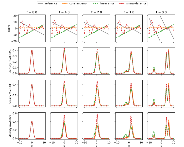
Figure 1. One dimensional test: Density estimations obtained by solving the Fokker-Planck PDE (LABEL:e:defUV) numerically with various artificial score errors. From top to bottom: score, estimated density with $\delta=0.005,\,0.01,\,0.02$. From left to right estimated $q_{t}$ at $t=8,\,4,\,2,\,1,\,0$.

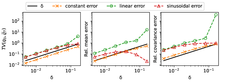
Figure 2. One dimensional test: convergence of the density estimations obtained by solving the Fokker-Planck PDE (LABEL:e:defUV) numerically with various artificial score errors.

Then, we investigate the convergence of the probability ODE flow by integrating the deterministic reverse process (6). The corresponding score function, reference density $q_{t}$, and estimated density $\widehat{\varrho}_{T-t}$ with various imperfect score estimations are depicted in Fig. 3. Kernel density estimates are computed with bandwidth determined by Silverman’s rule [34] $\Bigl{(}\frac{4}{J(d+2)}\Bigr{)}^{1/(d+4)}(1-\frac{t}{2T})$ (interpolating from $0.5$ to $1$). Notably, the estimated densities closely resemble the PDE solution (See Fig. 1), highlighting the significant efficiency of the time integrator with such small numbers of time steps. The convergence rate, evaluated in terms of the total variation TV$(q_{0},\widehat{\varrho}_{T})$, relative mean error, and relative covariance error, is depicted in Fig. 4. The linear relationship between these errors and $\delta$ (or $h^{2}$) is clearly demonstrated.

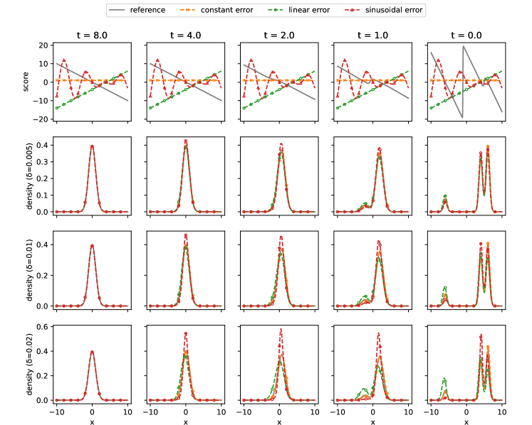
Figure 3. One dimensional test: density estimations obtained by solving the probability flow ODE with Heun’s method with various artificial score errors. From top to bottom: score, estimated density with $\delta=0.005,\,0.01,\,0.02$. From left to right estimated $q_{t}$ at $t=8,\,4,\,2,\,1,\,0$.

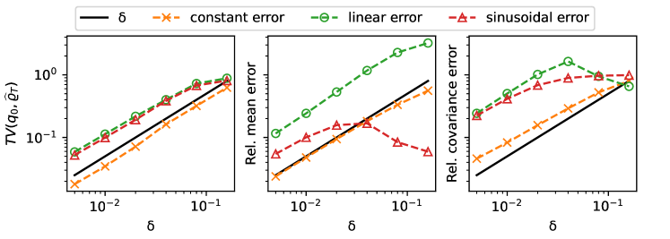
Figure 4. One dimensional test: convergence of the density estimations obtained by solving the probability flow ODE with Heun’s method, where $h^{2}\approx\delta$ with various artificial score errors.

4.2. High Dimensional Test

Finally, we consider $d$ dimensional 5-mode Gaussian mixtures (15). The weights are sampled uniformly $w_{k}\sim$ Uniform$[0,1]$ are then normalized to sum to 1. The means are generated from a Gaussian distribution, $m_{k}\sim\mathcal{N}(0,3^{2}{\mathbb{I}}_{d})$, and the covariance matrices $C_{k}$ are generated as $C_{k}=\frac{1}{8}(W_{k}^{T}W_{k}/d+{\mathbb{I}}_{d})$ with $(W_{k})_{ij}\sim\mathcal{N}(0,1)$ for $i,j=1,\,\cdots,\,d$.

We investigate the convergence of the ODE flow by integrating the deterministic reverse process (6) with the same setup as before. For $d=128$, we visualize the results in terms of the marginal density for the first dimension, including its score, reference density $q^{1}_{t}$, and estimated density $\widehat{\varrho}^{1}_{T-t}$ with various artificial score errors, as depicted in Fig. 5. We compute kernel density estimates with the bandwidth determined by the same Silverman’s rule [34] as in Section 4.1. Surprisingly, the estimated densities are as good as those of the one-dimensional test (See Fig. 3). We further consider $d=8$ and $32$ by generating the target density $q_{0}$ through marginalizing the 128-dimensional Gaussian mixture target density. The convergence rate, evaluated in terms of the total variation of the marginal density TV$(q^{1}_{0},\widehat{\varrho}^{1}_{T})$, relative mean error, and relative covariance error, is depicted in Fig. 6. The linear relationship between these errors and $\delta$ (or $h^{2}$) is clearly demonstrated. Additionally, we also explore the scenario without score matching errors for comprehensive analysis. The convergence rate, evaluated using the same error indicators, is presented in Fig. 7, showing the quadratic relationship with $h^{2}$. Notably, in this high dimensional test study, we do not observe any dimension dependence.

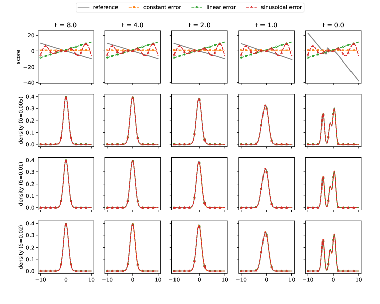
Figure 5. 128 dimensional test: marginal densities obtained by solving the probability flow ODE with Heun’s method with various artificial score errors. From top to bottom: score, estimated densities with $\delta=0.005,\,0.01,\,0.02$. From left to right estimated $q_{t}$ at $t=8,\,4,\,2,\,1,\,0$.

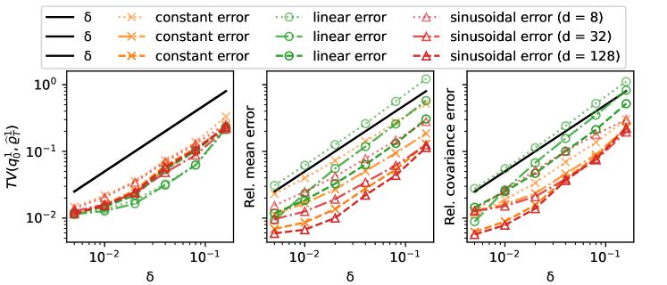
Figure 6. High dimensional test: convergence of the density estimations obtained by solving the probability flow ODE with Heun’s method, where $h^{2}\approx\delta$ with various artificial score errors. The dotted lines, dash dot lines and dashed lines indicate $d=8,32$ and, $128$ dimension tests, respectively.

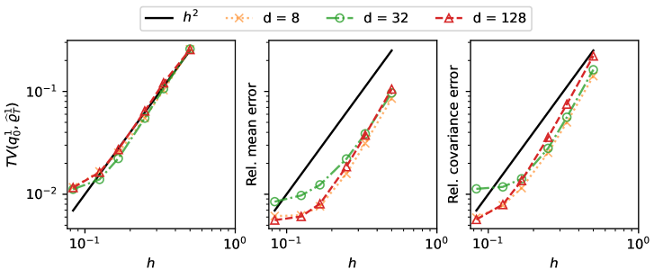
Figure 7. High dimensional test: convergence of the density estimations with no score errors obtained by solving the probability flow ODE with Heun’s method, across different time step sizes $h$. The dotted cross lines, dash dot circle lines and dashed triangle lines indicate $d=8,32$ and, $128$ dimension tests, respectively.

5. Conclusion

In this study, we have investigated the convergence of score-based generative model based on the probability flow ODE, both theoretically and numerically. Our analysis provided theoretical convergence guarantees at both continuous and discrete levels. Additionally, our numerical studies, conducted on problems up to 128 dimensions, provided empirical verification of our theoretical findings. One notable observation is the superior error bound of $\mathcal{O}(\delta+h^{p})$, indicating potential sharper estimations with improved dimension and score matching error dependence. Moreover, conducting rigorous numerical-based analyses with neural network-based score estimation errors is also a focus for future research.

Acknowledgments DZH is supported by the high-performance computing platform of Peking University. JH is supported by NSF grant DMS-2331096, and the Sloan research fellowship. ZJL would like to thank Professor Guido De Philippis for the insightful discussions.

Appendix A Total Variation Estimates along Probability Flow

In this section, we prove the following general theorem for continuity equations, which is independent of the particular choice of $U_{t},\widehat{U}_{t}$ (equivalently, $V_{T-t},\widehat{V}_{T-t}$) in (LABEL:e:defUV).

Theorem A.1.

Fix any $0<\tau<T$. Let $\widehat{q}_{t}(x),q_{t}(x)\in C^{1}([\tau,T]\times\mathbb{R}^{d})\cap L^{1}([\tau,T]\times\mathbb{R}^{d})$ solve the following two continuity equations on $\mathbb{R}^{d}$ respectively,

$$\partial_{t}q_{t}=\nabla\cdot(U_{t}q_{t}),\quad\partial_{t}\widehat{q}_{t}=\nabla\cdot(\widehat{U}_{t}\widehat{q}_{t}).$$

We also assume that for $t\in[\tau,T]$, $U_{t},\widehat{U}_{t}$ are locally Lipschitz on $\mathbb{R}^{d}$. Then, if we denote $\delta_{t}(x)\coloneq\widehat{U}_{t}(x)-U_{t}(x)$, $\widehat{\varepsilon}_{t}(x)\coloneq\widehat{q}_{t}(x)-q_{t}(x)$, we have that,

$$\bigg{|}\int_{\mathbb{R}^{d}}|\widehat{\varepsilon}_{\tau}(x)|\ {\rm d}x-\int_{\mathbb{R}^{d}}|\widehat{\varepsilon}_{T}(x)|\ {\rm d}x\bigg{|}\leq\int_{\tau}^{T}E(t)\ {\rm d}t,\quad\text{with }E(t)\coloneq\int_{\mathbb{R}^{d}}\bigg{|}(\nabla\cdot(q_{t}\delta_{t}))(x)\bigg{|}\ {\rm d}x.$$

First Proof.

Fix this given $\tau>0$. For $t>0$, we define the total variation between $\widehat{q}_{t}(x)$ and $q_{t}(x)$ as

(17) $$f(t)\coloneq\int_{\mathbb{R}^{d}}|\widehat{\varepsilon}_{t+\tau}(x)|\ {\rm d}x.$$

We use $x_{t}\coloneq T_{t}(x)$ to denote the solution of the ODE (also called the characteristic line)

$$\frac{{\rm d}}{{\rm d}t}T_{t}(x)=-\widehat{U}_{\tau+t}(T_{t}(x)),$$

with the initial data $x_{0}=T_{0}(x)=x$. We notice that, by change of variables (we can do this because $\widehat{U}_{t}$ is locally Lipschitz on $\mathbb{R}^{d}$. So, $T_{t}$ is a diffeomorphism of $\mathbb{R}^{d}$),

$$f(t)=\int_{\mathbb{R}^{d}}|\widehat{\varepsilon}_{t+\tau}(x_{t})|JT_{t}(x)\ {\rm d}x,$$

where $JT_{t}(x)=|\det(\nabla T_{t}(x))|$. A direct computation shows that

$$\frac{{\rm d}}{{\rm d}t}\widehat{\varepsilon}_{t+\tau}(x)=(\nabla\cdot(\widehat{U}_{t+\tau}\widehat{\varepsilon}_{t+\tau}))(x)+(\nabla\cdot(q_{t+\tau}\delta_{t+\tau}))(x).$$

Hence,

$$\frac{{\rm d}}{{\rm d}t}\widehat{\varepsilon}_{t+\tau}(x_{t})=(\nabla\cdot\widehat{U}_{t+\tau})(x_{t})\cdot\widehat{\varepsilon}_{t+\tau}(x_{t})+(\nabla\cdot(q_{t+\tau}\delta_{t+\tau}))(x_{t}).$$

Jacobi’s formula gives that

$$\frac{{\rm d}}{{\rm d}t}\det(\nabla T_{t}(x))=\mathrm{trace}\bigg{(}\bigg{(}\frac{{\rm d}}{{\rm d}t}\nabla T_{t}(x)\bigg{)}\cdot{\bigg{(}\nabla T_{t}(x)\bigg{)}}^{-1}\bigg{)}\cdot\det(\nabla T_{t}(x)).$$

We also notice that

$$\frac{{\rm d}}{{\rm d}t}\nabla T_{t}(x)=\nabla\frac{{\rm d}}{{\rm d}t}T_{t}(x)=-\nabla(\widehat{U}_{\tau+t}(T_{t}(x)))=-(\nabla\widehat{U}_{\tau+t})(T_{t}(x))\cdot\nabla T_{t}(x).$$

Hence,

$$\frac{{\rm d}}{{\rm d}t}\det(\nabla T_{t}(x))=-\mathrm{trace}\bigg{(}(\nabla\widehat{U}_{\tau+t})(T_{t}(x))\bigg{)}\cdot\det(\nabla T_{t}(x))=-(\nabla\cdot\widehat{U}_{\tau+t})(T_{t}(x))\cdot\det(\nabla T_{t}(x)).$$

So,

$$\begin{split}\bigg{|}\frac{{\rm d}}{{\rm d}t}f(t)\bigg{|}&\leq\int_{\mathbb{R}^{d}}\bigg{|}\big{[}(\nabla\cdot\widehat{U}_{t+\tau})(x_{t})\cdot\widehat{\varepsilon}_{t+\tau}(x_{t})+(\nabla\cdot(q_{t+\tau}\delta_{t+\tau}))(x_{t})\big{]}\cdot\det(\nabla T_{t}(x))\\ &\quad+\widehat{\varepsilon}_{t+\tau}(x_{t})\cdot(-(\nabla\cdot\widehat{U}_{\tau+t})(T_{t}(x)))\cdot\det(\nabla T_{t}(x))\bigg{|}\ {\rm d}x\\ &=\int_{\mathbb{R}^{d}}\bigg{|}(\nabla\cdot(q_{t+\tau}\delta_{t+\tau}))(x_{t})\bigg{|}\cdot JT_{t}(x)\ {\rm d}x\\ &=\int_{\mathbb{R}^{d}}\bigg{|}(\nabla\cdot(q_{t+\tau}\delta_{t+\tau}))(x)\bigg{|}\ {\rm d}x=E(t+\tau),\end{split}$$

where the second last equality is by change of variables again. Hence, for any $t^{\prime}>0$,

(18) $$f(0)\leq\int_{0}^{t^{\prime}}E(t+\tau)\ {\rm d}t+f(t^{\prime}).$$

One can also use the characteristic line method starting from $t=T$ to $t=\tau$, and then obtain an inverse inequality. Hence, we finish the proof of the theorem. ∎

Remark A.2.

Notice that in this first proof, we exchange the order of integrals and derivatives. We can do this in our problem setting (LABEL:e:defUV), because by Assumption 3.1, $\mu_{\ast}$ is compactly supported, so $q_{t}(x)$ always has a exponential tail as $\|x\|\to+\infty$. $\widehat{q}_{t}(x)$ also has such a property by our Lemma B.6.

Indeed, one can prove the following more general theorem with reasonable assumptions, essentially verbatim, by the same method.

Theorem A.3.

Fix any $0<\tau<T$. Let $p_{t}(x)\in C^{1}([\tau,T]\times\mathbb{R}^{d})\cap L^{1}([\tau,T]\times\mathbb{R}^{d})$ solve the following continuity equation on $\mathbb{R}^{d}$ with $h_{t}(x)\in L^{1}([\tau,T]\times\mathbb{R}^{d})$,

$$\partial_{t}p_{t}(x)=(\nabla\cdot(Z_{t}p_{t}))(x)+h_{t}(x).$$

We also assume that for $t\in[\tau,T]$, $Z_{t}$ is locally Lipschitz on $\mathbb{R}^{d}$. Then, for almost all $t\in[\tau,T]$, we have that,

$$\bigg{|}\frac{{\rm d}}{{\rm d}t}\int_{\mathbb{R}^{d}}|p_{t}(x)|\ {\rm d}x\bigg{|}\leq\int_{\mathbb{R}^{d}}|h_{t}(x)|\ {\rm d}x.$$

Hence,

$$\bigg{|}\int_{\mathbb{R}^{d}}|p_{\tau}(x)|{\rm d}x-\int_{\mathbb{R}^{d}}|p_{T}(x)|{\rm d}x\bigg{|}\leq\int_{\tau}^{T}\int_{\mathbb{R}^{d}}|h_{t}(x)|\ {\rm d}x.$$

Remark A.4.

We will prove a Gagliardo-Nirenberg interpolation inequality with dimension free constants in Lemma C.1. With this inequality, if one can know that $\int_{\mathbb{R}^{d}}|\partial^{2}_{ii}p_{\tau}(x)|{\rm d}x$ is bounded for some $i\in\llbracket 1,d\rrbracket$, then one can use Lemma C.1 to see that $\int_{\mathbb{R}^{d}}|\partial_{i}p_{\tau}(x)|{\rm d}x$ is also small if $\int_{\mathbb{R}^{d}}|p_{\tau}(x)|{\rm d}x$ is small. Similar arguments work for higher order derivatives of $p_{\tau}(x)$. Moreover, if we can conclude that the $W^{k,1}(\mathbb{R}^{d})$-norms of $p_{\tau}(x)$ is small, where $W^{k,1}$ means Sobolev spaces, we can use Sobolev inequalities to conclude that the $W^{k-1,r}(\mathbb{R}^{d})$-norms of $p_{\tau}(x)$ for a corresponding $r>1$ is also mall. In particular, we can conclude that the $L^{r}(\mathbb{R}^{d})$-norm of $p_{\tau}(x)$ is small.

Before we give the second proof of Theorem A.1 and Theorem A.3, we need to explain our intuition a little bit. With those notations in Theore A.3, we notice that for

$$g(t)\coloneq\int_{\mathbb{R}^{d}}|p_{t}(x)|\ {\rm d}x,$$

we have that

$$\frac{{\rm d}}{{\rm d}t}g(t)=\int_{\mathbb{R}^{d}}\operatorname{sign}(p_{t}(x))\frac{{\rm d}}{{\rm d}t}p_{t}(x)\ {\rm d}x=\int_{\{p_{t}\geq 0\}}\frac{{\rm d}}{{\rm d}t}p_{t}(x)\ {\rm d}x-\int_{\{p_{t}<0\}}\frac{{\rm d}}{{\rm d}t}p_{t}(x)\ {\rm d}x.$$

If the boundary $\partial\{p_{t}\geq 0\}$ consists of $(d-1)$-dimensional piecewise smooth submanifolds (or at least rectifiable sets), then by the divergence theorem, we know that

$$\int_{\{p_{t}\geq 0\}}(\nabla\cdot(Z_{t}p_{t}))(x)\ {\rm d}x=\int_{\partial\{p_{t}\geq 0\}}\textbf{n}(x)\cdot(Z_{t}p_{t})(x)\ d\mathcal{H}^{d-1}(x)=0,$$

where $\textbf{n}(x)$ is the unit outer normal vector and $\mathcal{H}^{d-1}(\cdot)$ is the $(d-1)$-dimensional surface measure. Similarly,

$$\int_{\{p_{t}<0\}}(\nabla\cdot(Z_{t}p_{t}))(x)\ {\rm d}x=0.$$

So,

$$\frac{{\rm d}}{{\rm d}t}g(t)=\int_{\mathbb{R}^{d}}\operatorname{sign}(p_{t}(x))h_{t}(x)\ {\rm d}x,\ \text{and }\bigg{|}\frac{{\rm d}}{{\rm d}t}g(t)\bigg{|}\leq\int_{\mathbb{R}^{d}}|h_{t}(x)|\ {\rm d}x.$$

However, in general, we cannot know whether the boundary set $\partial\{p_{t}\geq 0\}$ is always of $(d-1)$-dimension. For an arbitrarily given smooth function, its zero level set can also be arbitrarily strange and does not necessarily need to be of $(d-1)$-dimension.

The following second proof of Theorem A.3 is inspired by [3] and the communication with Professor Guido De Philippis. We also assume that $(\|Z_{t}(x)\|\cdot|p_{t}(x)|)\in L^{1}(\mathbb{R}^{d}\times[\tau,T])$.

Second Proof.

Let $a>0$. We let $\beta_{a}(s)=\sqrt{a^{2}+s^{2}}$ be a function on $\mathbb{R}$ which approximates the function $|s|$ as $a\to 0^{+}$. Then, the function $p_{a,t}(x)\coloneq\beta_{a}(p_{t}(x))$ on $\mathbb{R}^{d}$ solves the equation

$$\begin{split}\partial_{t}p_{a,t}(x)&=((\nabla\cdot Z_{t})(x))p_{t}(x)\beta_{a}^{\prime}(p_{t}(x))+Z_{t}(x)\cdot\nabla p_{a,t}(x)+h_{t}(x)\beta_{a}^{\prime}(p_{t}(x))\\ &=\nabla\cdot(Z_{t}(x)p_{a,t}(x))+((\nabla\cdot Z_{t})(x))[p_{t}(x)\beta_{a}^{\prime}(p_{t}(x))-p_{a,t}(x)]+h_{t}(x)\beta_{a}^{\prime}(p_{t}(x)).\end{split}$$

For any $R>0$, consider the integral of the above equation on the ball $B_{R}\coloneq B_{R}(0)\subset\mathbb{R}^{d}$, we have that

$$\begin{split}\frac{{\rm d}}{{\rm d}t}\int_{B_{R}}p_{a,t}(x){\rm d}x&=\int_{\partial B_{R}}(Z_{t}(x)p_{a,t}(x))\cdot\frac{x}{\|x\|}d\mathcal{H}^{d-1}(x)+\int_{B_{R}}((\nabla\cdot Z_{t})(x))[p_{t}(x)\beta_{a}^{\prime}(p_{t}(x))-p_{a,t}(x)]\ {\rm d}x\\ &\quad+\int_{B_{R}}h_{t}(x)\beta_{a}^{\prime}(p_{t}(x))\ {\rm d}x,\end{split}$$

and then for any $t^{\prime},t^{\prime\prime}\in[\tau,T]$,

$$\begin{split}\bigg{|}\int_{B_{R}}p_{a,t^{\prime\prime}}(x){\rm d}x-\int_{B_{R}}p_{a,t^{\prime}}(x){\rm d}x\bigg{|}&=\bigg{|}\int_{t^{\prime\prime}}^{t^{\prime}}\int_{\partial B_{R}}(Z_{t}(x)p_{a,t}(x))\cdot\frac{x}{\|x\|}d\mathcal{H}^{d-1}(x){\rm d}t\\ &\quad+\int_{t^{\prime\prime}}^{t^{\prime}}\int_{B_{R}}((\nabla\cdot Z_{t})(x))[p_{t}(x)\beta_{a}^{\prime}(p_{t}(x))-p_{a,t}(x)]\ {\rm d}x{\rm d}t\\ &\quad+\int_{t^{\prime\prime}}^{t^{\prime}}\int_{B_{R}}h_{t}(x)\beta_{a}^{\prime}(p_{t}(x))\ {\rm d}x{\rm d}t\bigg{|}.\end{split}$$

Notice that $|\beta_{a}^{\prime}(s)|=\frac{|s|}{\sqrt{a^{2}+s^{2}}}\leq 1$, $|p_{t}(x)\beta_{a}^{\prime}(p_{t}(x))-p_{a,t}(x)|=\frac{a^{2}}{\sqrt{a^{2}+p_{t}(x)^{2}}}\leq 1$, and for any given $x\in B_{R}$, $\lim_{a\to 0^{+}}\frac{a^{2}}{\sqrt{a^{2}+p_{t}(x)^{2}}}=0$. By the dominated convergence theorem, we can let $a\to 0^{+}$ on both sides and obtain that

$$\begin{split}\bigg{|}\int_{B_{R}}|p_{t^{\prime\prime}}(x)|{\rm d}x-\int_{B_{R}}|p_{t^{\prime}}(x)|{\rm d}x\bigg{|}&=\bigg{|}\int_{t^{\prime\prime}}^{t^{\prime}}\int_{\partial B_{R}}(Z_{t}(x)|p_{t}(x)|)\cdot\frac{x}{\|x\|}d\mathcal{H}^{d-1}(x){\rm d}t\\ &\quad+\int_{t^{\prime\prime}}^{t^{\prime}}\int_{B_{R}}((\nabla\cdot Z_{t})(x))\cdot 0\ {\rm d}x{\rm d}t\\ &\quad+\int_{t^{\prime\prime}}^{t^{\prime}}\int_{B_{R}}h_{t}(x)\operatorname{sign}(p_{t}(x))\ {\rm d}x{\rm d}t\bigg{|}\\ &\leq\int_{t^{\prime\prime}}^{t^{\prime}}\int_{\partial B_{R}}\|Z_{t}(x)\|\cdot|p_{t}(x)|d\mathcal{H}^{d-1}(x){\rm d}t\\ &\quad+\int_{t^{\prime\prime}}^{t^{\prime}}\int_{B_{R}}|h_{t}(x)|\ {\rm d}x{\rm d}t.\end{split}$$

Because we assumed that $(\|Z_{t}(x)\|\cdot|p_{t}(x)|)\in L^{1}(\mathbb{R}^{d}\times[\tau,T])$, we can choose a sequence $\{R_{j}\}$ with $R_{j}\to+\infty$, such that the first term on the right hand side goes to $0$. So, by the monotone convergence theorem, after passing $R_{j}\to+\infty$, we obtain that for any $t^{\prime},t^{\prime\prime}\in[\tau,T]$,

$$\bigg{|}\int_{\mathbb{R}^{d}}|p_{t^{\prime\prime}}(x)|{\rm d}x-\int_{\mathbb{R}^{d}}|p_{t^{\prime}}(x)|{\rm d}x\bigg{|}\leq\int_{t^{\prime\prime}}^{t^{\prime}}\int_{\mathbb{R}^{d}}|h_{t}(x)|\ {\rm d}x{\rm d}t.$$

∎

Appendix B Preliminary Estimates on Forward and Backward Density

In this section, $U_{t},\widehat{U}_{t}$ are defined as in (LABEL:e:defUV). Under 3.1, we take $\lambda_{t}=e^{-t}$ and $\sigma_{t}=\sqrt{1-\lambda_{t}^{2}}$ ($t>0$), and we also assume that

(19) $$q_{t}(y)\coloneq\int_{\mathbb{R}^{d}}\frac{1}{{(\sqrt{2\pi}\sigma_{t})}^{d}}\cdot e^{-\frac{\|y-x\|^{2}}{2{\sigma_{t}}^{2}}}\cdot\mu_{\ast}\bigg{(}\frac{x}{\lambda_{t}}\bigg{)}\frac{1}{{\lambda_{t}}^{d}}\ {\rm d}x,$$

which satisfies the first-order PDE: $\partial_{t}q_{t}=\nabla\cdot(U_{t}q_{t})$ for $U_{t}=x+\nabla\log q_{t}(x)$. We remark that although we use the notation $\mu_{\ast}(x/\lambda_{t}^{d})/\lambda_{t}^{d}$ in the definition (19) of $q_{t}$, because the data distribution $\mu_{\ast}$ can be supported on a submanifold $K_{\ast}$, or more general lower dimensional rectifiable sets, the meaning of it is actually the push-forward measure defined by $(\lambda_{t})_{\#}\mu_{\ast}(A)\coloneq\mu_{\ast}(\lambda_{t}^{-1}A)$ for any measurable set $A\subset\mathbb{R}^{d}$. So, the rescaling factor $\lambda_{t}^{d}$ is actually $\lambda_{t}^{k}$ for $k\leq d$ when $K_{\ast}$ is a $k-$dimensional submanifold in $\mathbb{R}^{d}$. But this notation doesn’t affect our computations. As readers will see, the only property we will use is that in the integrand of (19), $x/\lambda_{t}\in K_{\ast}$ and hence $\|x\|_{\infty}\leq\lambda_{t}D$.

Example B.1.

When $\mu_{\ast}$ is the delta mass at a point $y_{0}\in\mathbb{R}^{d}$, then for $t>0$,

$$q_{t}(y)=\frac{1}{{(\sqrt{2\pi}\sigma_{t})}^{d}}\cdot e^{-\frac{\|y-y_{0}\|^{2}}{2{\sigma_{t}}^{2}}},\quad\nabla q_{t}(y)=-\frac{y-y_{0}}{\sigma_{t}^{2}}q_{t}(y),\quad\nabla^{2}\log q_{t}(y)=-\frac{1}{\sigma_{t}^{2}}\cdot{\mathbb{I}}_{d}.$$

We notice that as $t\to 0^{+}$, the derivatives of $\log q_{t}(y)$ blow up.

Example B.2.

When $\mu_{\ast}$ is the unit $2$-sphere $\mathbb{S}^{2}\subset\mathbb{R}^{3}\subset\mathbb{R}^{d}$, if we write $y=(y^{\prime},y^{\prime\prime})\in\mathbb{R}^{3}\times\mathbb{R}^{d-3}$ and $y^{\prime}=(y_{1},y_{2},y_{3})$, a direct computation shows that

$$q_{t}(y)=\frac{2\pi}{{(\sqrt{2\pi}\sigma_{t})}^{d}}\cdot e^{-\frac{\|y\|^{2}+\lambda_{t}^{2}}{2{\sigma_{t}}^{2}}}\cdot\frac{\sigma_{t}^{2}}{\lambda_{t}\|y^{\prime}\|}\cdot\bigg{(}e^{\frac{\lambda_{t}\|y^{\prime}\|}{\sigma_{t}^{2}}}-e^{-\frac{\lambda_{t}\|y^{\prime}\|}{\sigma_{t}^{2}}}\bigg{)}.$$

The derivatives of $\log q_{t}(y)$ also blow up as $t\to 0^{+}$ by a direct computation.

In general, we have the following estimates for space directions derivatives of $q_{t}(y)$ and $\log q_{t}(y)$. An interesting fact is that the upper bound in the statement of Lemma B.3 is uniform for $y\in\mathbb{R}^{d}$.

Lemma B.3.

For any $p\geq 3$, any $y\in\mathbb{R}^{d}$ and any $t>0$,

(20) $$\|\nabla^{p}\log q_{t}(y)\|_{\infty}\leq(4p!)\frac{{\lambda_{t}}^{p}D^{p}}{{\sigma_{t}}^{2p}}.$$

Also, for any $i,j$,

$$|\partial_{y_{i}}\log q_{t}(y)|\leq\frac{|y_{i}|+\lambda_{t}D}{\sigma_{t}^{2}},\text{ and }|\partial^{2}_{y_{i}y_{j}}\log q_{t}(y)|\leq\frac{\delta_{ij}}{\sigma_{t}^{2}}+2\frac{\lambda_{t}^{2}D^{2}}{\sigma_{t}^{4}}.$$

Proof.

For simplicity, for a function $f(x)$ defined on $\mathbb{R}^{d}$, we denote

(21) $$\langle f(x)\rangle\coloneq\int_{\mathbb{R}^{d}}f(x)\ {\rm d}(\lambda_{t})_{\#}\mu_{\ast}(x)=\int_{\mathbb{R}^{d}}f(x)\mu_{\ast}\bigg{(}\frac{x}{\lambda_{t}}\bigg{)}\frac{1}{{\lambda_{t}}^{d}}\ {\rm d}x.$$

Hence, $q_{t}(y)=\langle\frac{1}{{(\sqrt{2\pi}\sigma_{t})}^{d}}\cdot e^{-\frac{\|y-x\|^{2}}{2{\sigma_{t}}^{2}}}\rangle$. For simplicity, we discuss the derivatives of the logarithm of the $y$-function $h(y)\coloneq\langle e^{a{\|y+x\|}^{2}}\rangle$, where $a\in\mathbb{R}$ is a constant. We will choose $a=-\frac{1}{2\sigma_{t}^{2}}$ finally, and the difference between $\|y-x\|^{2}$ and $\|y+x\|^{2}=\|-y-x\|^{2}$ doesn’t influence the $\|\cdot\|_{\infty}$-norms of derivatives.

We first compute the first and second derivatives of $\log h(y)$. We notice that

(22) $$\partial_{i}h(y)=2a\langle(y_{i}+x_{i})e^{a{\|y+x\|}^{2}}\rangle=2ay_{i}h(y)+2a\langle x_{i}e^{a{\|y+x\|}^{2}}\rangle.$$

So,

(23) $$\partial^{2}_{ij}h(y) =2a\delta_{ij}h(y)+2ay_{j}(2ay_{i}h(y)+2a\langle x_{i}e^{a{\|y+x\|}^{2}}\rangle)+4a^{2}\langle(x_{i}+y_{i})x_{j}e^{a{\|y+x\|}^{2}}\rangle$$

(24) $$=2a\delta_{ij}h(y)+4a^{2}y_{i}y_{j}h(y)+4a^{2}y_{i}\langle(x_{j}e^{a{\|y+x\|}^{2}}\rangle+4a^{2}y_{j}\langle x_{i}e^{a{\|y+x\|}^{2}}\rangle+4a^{2}\langle x_{i}x_{j}e^{a{\|y+x\|}^{2}}\rangle.$$

Hence,

(25) $$\begin{split}\partial^{2}_{ij}\log h(y)&=\frac{\partial^{2}_{ij}h(y)h(y)-\partial_{i}h(y)\partial_{j}h(y)}{h(y)^{2}}\\ &=2a\delta_{ij}+4a^{2}\frac{\langle x_{i}x_{j}e^{a{\|y+x\|}^{2}}\rangle h(y)-\langle x_{i}e^{a{\|y+x\|}^{2}}\rangle\langle x_{j}e^{a{\|y+x\|}^{2}}\rangle}{h(y)^{2}}.\end{split}$$

Before we compute higher order derivatives of $\log h(y)$, we first illustrate how we obtain an upper bound for $\partial^{2}_{ij}\log h(y)$. Notice that in the definition of $\langle f(x)\rangle$ in (21), because $\mu_{\ast}$ has a compact support $K_{\ast}$, the $x$ in the integrand satisfies that $x\in\lambda_{t}K_{\ast}$. Hence, in the integrand of (21), $\|x\|_{\infty}\leq\lambda_{t}D$ by Assumption 3.1. So, $|\langle x_{i}e^{a{\|y+x\|}^{2}}\rangle|\leq\lambda_{t}Dh(y)$, $|\langle x_{i}x_{j}e^{a{\|y+x\|}^{2}}\rangle|\leq\lambda_{t}^{2}D^{2}h(y)$. So, $|\partial^{2}_{ij}\log h(y)|\leq 2a\delta_{ij}+8a^{2}\lambda_{t}^{2}D^{2}$.

Then, we compute $\nabla^{p}\log q_{t}(y)$ for $p\geq 3$. We use induction to show that in the expression of $\nabla^{p}\log h(y)$, there is no polynomial term of $y$ like we have seen in (25). Assume that for an $m\in\mathbb{Z}_{+}$, and for any multi-index $\alpha$ with $|\alpha|=m$, the derivative $\partial_{y}^{\alpha}\log h(y)$ has a form

$$\partial_{y}^{\alpha}\log h(y)={(2a)}^{m}\frac{P_{\alpha}(y)}{h(y)^{m}},$$

where $P_{\alpha}(y)$ is the summation of at most $4(m-1)!-2$ terms, where each term has a form

$$\pm\langle x^{\beta_{1}}e^{a{\|y+x\|}^{2}}\rangle\cdot\langle x^{\beta_{2}}e^{a{\|y+x\|}^{2}}\rangle\cdots\langle x^{\beta_{m}}e^{a{\|y+x\|}^{2}}\rangle,$$

and each $\beta_{i}$ is a multi-index and $|\beta_{1}|+|\beta_{2}|+\ldots+|\beta_{m}|=m$. This assumption is satisfied when $m=2$, because the derivative of the term $2a\delta_{ij}$ in (25) is zero so that we can omit this term. Then,

(26) $$\partial_{y_{1}}\partial_{y}^{\alpha}\log h(y)={(2a)}^{m}\partial_{y_{1}}\frac{P_{\alpha}(y)}{h(y)^{m}}={(2a)}^{m+1}\cdot\frac{\frac{1}{2a}\partial_{y_{1}}P_{\alpha}(y)h(y)-mP_{\alpha}(y)\langle(y_{1}+x_{1})e^{a{\|y+x\|}^{2}}\rangle}{h(y)^{m+1}}.$$

We notice that

$$\begin{split}&\frac{1}{2a}\partial_{y_{1}}\big{(}\langle x^{\beta_{1}}e^{a{\|y+x\|}^{2}}\rangle\cdot\langle x^{\beta_{2}}e^{a{\|y+x\|}^{2}}\rangle\cdots\langle x^{\beta_{m}}e^{a{\|y+x\|}^{2}}\rangle\big{)}\\ &=my_{1}\langle x^{\beta_{1}}e^{a{\|y+x\|}^{2}}\rangle\cdot\langle x^{\beta_{2}}e^{a{\|y+x\|}^{2}}\rangle\cdots\langle x^{\beta_{m}}e^{a{\|y+x\|}^{2}}\rangle\\ &\quad+\langle x_{1}x^{\beta_{1}}e^{a{\|y+x\|}^{2}}\rangle\cdot\langle x^{\beta_{2}}e^{a{\|y+x\|}^{2}}\rangle\cdots\langle x^{\beta_{m}}e^{a{\|y+x\|}^{2}}\rangle\\ &\quad+\langle x^{\beta_{1}}e^{a{\|y+x\|}^{2}}\rangle\cdot\langle x_{1}x^{\beta_{2}}e^{a{\|y+x\|}^{2}}\rangle\cdots\langle x^{\beta_{m}}e^{a{\|y+x\|}^{2}}\rangle\\ &\quad+\ldots+\langle x^{\beta_{1}}e^{a{\|y+x\|}^{2}}\rangle\cdot\langle x^{\beta_{2}}e^{a{\|y+x\|}^{2}}\rangle\cdots\langle x_{1}x^{\beta_{m}}e^{a{\|y+x\|}^{2}}\rangle.\end{split}$$

Hence, $\frac{1}{2a}\partial_{y_{1}}P_{\alpha}(y)$ is of the form $my_{1}P_{\alpha}(y)+Q_{\alpha}(y)$, where $Q_{\alpha}(y)$ is the summation of at most $4(m-1)!-2$ terms without $y_{1}$ showing in the polynomial terms. We notice that those $y_{1}$ terms in the numerator of (26) will then cancel, and the remaining terms all look like

$$\pm\langle x^{\beta_{1}^{\prime}}e^{a{\|y+x\|}^{2}}\rangle\cdot\langle x^{\beta_{2}^{\prime}}e^{a{\|y+x\|}^{2}}\rangle\cdots\langle x^{\beta_{m+1}^{\prime}}e^{a{\|y+x\|}^{2}}\rangle,$$

where each $\beta_{i}^{\prime}$ is a multi-index and $|\beta_{1}^{\prime}|+|\beta_{2}^{\prime}|+\ldots+|\beta_{m+1}^{\prime}|=m+1$. The number of them is at most $m(4(m-1)!-2)+m=4m!-m\leq 4m!-2$ when $m\geq 2$. We then conclude the proof of Lemma B.3. ∎

The following lemma describes the situation when $t>0$ is very large.

Lemma B.4.

Let $q_{t}(y)$ be defined in (19), and let

$$g(y)\coloneq\frac{1}{{(\sqrt{2\pi})}^{d}}\cdot e^{-\frac{\|y\|^{2}}{2}}.$$

Then, we have that for $t>0$,

(27) $$\int_{\mathbb{R}^{d}}|q_{t}(y)-g(y)|{\rm d}y\leq\frac{2d(1-\sigma_{t})}{{\sigma_{t}}^{d+3}}+\lambda_{t}\sqrt{d}D\frac{4+\lambda_{t}\sqrt{d}D}{\sigma_{t}^{2}}\cdot e^{\frac{\lambda_{t}^{2}dD^{2}}{2{\sigma_{t}}^{2}}}.$$

In particular, there exists a universal constant $C_{u}>0$, such that

(28) $$\int_{\mathbb{R}^{d}}|q_{t}(y)-g(y)|{\rm d}y\leq C_{u}e^{-t}\sqrt{d}D,$$

which goes to $0$ exponentially as $t\rightarrow+\infty$.

Proof.

Because one can write

$$q_{t}(y)=\int_{\mathbb{R}^{d}}\frac{1}{{(\sqrt{2\pi}\sigma_{t})}^{d}}\cdot e^{-\frac{\|y-\lambda_{t}x\|^{2}}{2{\sigma_{t}}^{2}}}\ d\mu_{\ast}(x),$$

and $\int_{\mathbb{R}^{d}}d\mu_{\ast}(x)=1$, we see that

(29) $$\begin{split}\int_{\mathbb{R}^{d}}|q_{t}(y)-g(y)|{\rm d}y&=\int_{\mathbb{R}^{d}}\bigg{|}\int_{\mathbb{R}^{d}}\frac{1}{{(\sqrt{2\pi}\sigma_{t})}^{d}}\cdot e^{-\frac{\|y-\lambda_{t}x\|^{2}}{2{\sigma_{t}}^{2}}}-\frac{1}{{(\sqrt{2\pi})}^{d}}\cdot e^{-\frac{\|y\|^{2}}{2}}\ d\mu_{\ast}(x)\bigg{|}{\rm d}y\\ &\leq\int_{\mathbb{R}^{d}}\int_{\mathbb{R}^{d}}\bigg{|}\frac{1}{{(\sqrt{2\pi}\sigma_{t})}^{d}}\cdot e^{-\frac{\|y-\lambda_{t}x\|^{2}}{2{\sigma_{t}}^{2}}}-\frac{1}{{(\sqrt{2\pi})}^{d}}\cdot e^{-\frac{\|y\|^{2}}{2}}\bigg{|}{\rm d}y\ d\mu_{\ast}(x).\end{split}$$

We denote $y=(y_{1},y^{\prime})\in\mathbb{R}^{d}$, and we define the function

$$f(y,r)\coloneq\bigg{|}\frac{1}{{(\sqrt{2\pi}\sigma_{t})}^{d}}\cdot e^{-\frac{{|y_{1}-\lambda_{t}r|}^{2}+{\|y^{\prime}\|^{2}}}{2{\sigma_{t}}^{2}}}-\frac{1}{{(\sqrt{2\pi})}^{d}}\cdot e^{-\frac{\|y\|^{2}}{2}}\bigg{|}.$$

By the rotation symmetry, we see that the right hand side of (29) equals to

(30) $$\int_{\mathbb{R}^{d}}\int_{\mathbb{R}^{d}}f(y,\|x\|){\rm d}y\ d\mu_{\ast}(x).$$

Let’s first see what is $|\frac{{\rm d}}{{\rm d}r}f(y,r)|$ for $r\leq\sqrt{d}D$. A direct computation shows that

$$\begin{split}\bigg{|}\frac{{\rm d}}{{\rm d}r}f(y,r)\bigg{|}&=\frac{\lambda_{t}}{{(\sqrt{2\pi}\sigma_{t})}^{d}}\cdot\frac{|y_{1}-\lambda_{t}r|}{\sigma_{t}^{2}}\cdot e^{-\frac{{|y_{1}-\lambda_{t}r|}^{2}+{\|y^{\prime}\|^{2}}}{2{\sigma_{t}}^{2}}}\\ &\leq\frac{\lambda_{t}}{{(\sqrt{2\pi}\sigma_{t})}^{d}}\cdot\frac{|y_{1}|+\lambda_{t}\sqrt{d}D}{\sigma_{t}^{2}}\cdot e^{-\frac{{\frac{1}{2}|y_{1}|}^{2}-\lambda_{t}^{2}dD^{2}+{\|y^{\prime}\|^{2}}}{2{\sigma_{t}}^{2}}}.\end{split}$$

So, (30) is bounded by

(31) $$\int_{\mathbb{R}^{d}}\int_{\mathbb{R}^{d}}f(y,0){\rm d}y\ d\mu_{\ast}(x)+\int_{\mathbb{R}^{d}}\int_{\mathbb{R}^{d}}\frac{\lambda_{t}\|x\|}{{(\sqrt{2\pi}\sigma_{t})}^{d}}\cdot\frac{|y_{1}|+\lambda_{t}\sqrt{d}D}{\sigma_{t}^{2}}\cdot e^{-\frac{{\frac{1}{2}|y_{1}|}^{2}-\lambda_{t}^{2}dD^{2}+{\|y^{\prime}\|^{2}}}{2{\sigma_{t}}^{2}}}{\rm d}y\ d\mu_{\ast}(x).$$

The second term in (31) is bounded by

(32) $$\int_{\mathbb{R}^{d}}\frac{\lambda_{t}\sqrt{d}D}{{(\sqrt{2\pi}\sigma_{t})}^{d}}\cdot\frac{|y_{1}|+\lambda_{t}\sqrt{d}D}{\sigma_{t}^{2}}\cdot e^{-\frac{{\frac{1}{2}|y_{1}|}^{2}-\lambda_{t}^{2}dD^{2}+{\|y^{\prime}\|^{2}}}{2{\sigma_{t}}^{2}}}{\rm d}y\leq\lambda_{t}\sqrt{d}D\frac{4+\lambda_{t}\sqrt{d}D}{\sigma_{t}^{2}}\cdot e^{\frac{\lambda_{t}^{2}dD^{2}}{2{\sigma_{t}}^{2}}},$$

which goes to $0$ exponentially as $t\to+\infty$ because $\lambda_{t}=e^{-t}$ and $\sigma_{t}^{2}=1-\lambda_{t}^{2}$.

The first term in (31) is

(33) $$\int_{\mathbb{R}^{d}}\bigg{|}\frac{1}{{(\sqrt{2\pi}\sigma_{t})}^{d}}\cdot e^{-\frac{{\|y\|^{2}}}{2{\sigma_{t}}^{2}}}-\frac{1}{{(\sqrt{2\pi})}^{d}}\cdot e^{-\frac{\|y\|^{2}}{2}}\bigg{|}{\rm d}y,$$

because $\int_{\mathbb{R}^{d}}d\mu_{\ast}(x)=1$. We define the function

$$h(y,\alpha)=\bigg{|}\frac{1}{{(\sqrt{2\pi}\alpha)}^{d}}\cdot e^{-\frac{{\|y\|^{2}}}{2{\alpha}^{2}}}-\frac{1}{{(\sqrt{2\pi})}^{d}}\cdot e^{-\frac{\|y\|^{2}}{2}}\bigg{|},$$

and then for $\alpha\in[0,1]$,

$$\bigg{|}\frac{{\rm d}}{{\rm d}\alpha}h(y,\alpha)\bigg{|}=\frac{1}{{(\sqrt{2\pi})}^{d}}\bigg{|}-d\frac{1}{\alpha^{d+1}}e^{-\frac{{\|y\|^{2}}}{2{\alpha}^{2}}}+\frac{1}{\alpha^{d}}e^{-\frac{{\|y\|^{2}}}{2{\alpha}^{2}}}\cdot\frac{\|y\|^{2}}{\alpha^{3}}\bigg{|}\leq\frac{e^{-\frac{{\|y\|^{2}}}{2{\alpha}^{2}}}}{{(\sqrt{2\pi})}^{d}\alpha^{d+3}}\cdot|d+{\|y\|}^{2}|.$$

Because $h(y,1)=0$, we see that (33) is bounded by

(34) $$\frac{(1-\sigma_{t})}{{\sigma_{t}}^{d+3}}\int_{\mathbb{R}^{d}}\frac{e^{-\frac{{\|y\|^{2}}}{2}}}{{(\sqrt{2\pi})}^{d}}\cdot|d+{\|y\|}^{2}|{\rm d}y=\frac{2d(1-\sigma_{t})}{{\sigma_{t}}^{d+3}},$$

which goes to $0$ exponentially as $t\to+\infty$ because $\sigma_{t}=\sqrt{1-e^{-2t}}$. The estimates (32) and (34) together give (27). Next we show (28). There are two cases: if $e^{-t}\sqrt{d}D\geq 1$, then (28) holds trivially, since the lefthand side is at most $2$. Otherwise $e^{-t}\sqrt{d}D\leq 1$, we have

$$\begin{split}&\phantom{{}={}}\frac{2d(1-\sigma_{t})}{{\sigma_{t}}^{d+3}}+\lambda_{t}\sqrt{d}D\frac{4+\lambda_{t}\sqrt{d}D}{\sigma_{t}^{2}}\cdot e^{\frac{\lambda_{t}^{2}dD^{2}}{2{\sigma_{t}}^{2}}}\leq\frac{2de^{-2t}}{\sigma_{t}^{2d}}+\frac{4e^{-t}\sqrt{d}D+(e^{-t}\sqrt{d}D)^{2}}{\sigma_{t}^{2}}\cdot e^{\frac{1}{2{\sigma_{t}}^{2}}}\\ &\leq\frac{2de^{-2t}}{\sigma_{t}^{2d}}+\frac{5e^{-t}\sqrt{d}D}{\sigma_{t}^{2}}e^{\frac{2}{3}}=\frac{2de^{-2t}}{(1-e^{-2t})^{d}}+\frac{5e^{-t}\sqrt{d}D}{1-e^{-2t}}e^{\frac{2}{3}}\\ &\leq\frac{2\sqrt{d}e^{-t}}{1-de^{-2t}}\cdot\sqrt{d}e^{-t}+\frac{5e^{-t}\sqrt{d}D}{1-e^{-2t}}e^{\frac{2}{3}}\leq C_{u}e^{-t}\sqrt{d}D,\end{split}$$

for a universal constant $C_{u}>0$. In the last inequality, we assume that $e^{-t}\leq\frac{1}{4\sqrt{d}}\leq\frac{1}{4}$. Otherwise, if $e^{-t}\geq\frac{1}{4\sqrt{d}}$, (28) also holds trivially. This finishes the proof of (28). ∎

When we prove our main theorem, Theorem 3.4, in the following Section C, we will assume that $\mu_{\ast}$ has a compact support $K_{\ast}$ and use Lemma B.3 to proceed the proof. On the other hand, as we have mentioned in Remark 3.5, our methods work under other assumptions on the initial data $\mu_{\ast}$, as long as under those assumptions, we can reasonably obtain the properties in Remark C.4. We next assume that $\mu_{\ast}$ is a Gaussian mixture and obtain an estimate similar to Lemma B.3.

Lemma B.5.

Assume that $\mu_{\ast}$ is a Gaussian mixture, i.e., we assume that

$$\mu_{\ast}(x)\coloneq\sum_{k=1}^{M}c_{k}\frac{1}{{(\sqrt{2\pi})}^{d}a_{k}}\cdot\exp{\bigg{(}-\frac{1}{2}(x-b_{k})\cdot A_{k}^{-1}(x-b_{k})\bigg{)}},$$

where $A_{k}$’s are positive definite matrices, $a_{k}\coloneq\sqrt{\det A_{k}}$, $b_{k}$’s are constant vectors in $\mathbb{R}^{d}$, $c_{k}>0$ and $\sum_{k=1}^{M}c_{k}=1$. Then, for any $\ell\in\mathbb{Z}_{+}$ and any multi-index $\alpha$ with $|\alpha|\leq\ell$, there is a constant $C(\ell,\mu_{\ast})$, depending on $\ell$ and $A_{k},b_{k}$ in the formula of $\mu_{\ast}$, such that for any $x\in\mathbb{R}^{d}$ and any $t\geq 0$,

(35) $$\frac{|\partial_{x}^{\alpha}q_{t}(x)|}{q_{t}(x)}\leq C(\ell,\mu_{\ast})\cdot\|x\|^{\ell}+C(\ell,\mu_{\ast}).$$

Proof.

A standard computation, by (19), shows that the density function of $q_{t}(x)$ is

$$q_{t}(x)\coloneq\sum_{k=1}^{M}c_{k}\frac{1}{{(\sqrt{2\pi})}^{d}\cdot a_{k}(t)}\cdot\exp{\bigg{(}-\frac{1}{2}(x-b_{k}(t))\cdot A_{k}(t)^{-1}(x-b_{k}(t))\bigg{)}},$$

where $A_{k}(t)=\lambda_{t}^{2}A_{k}+\sigma_{t}^{2}{\mathbb{I}}_{d}$, $b_{k}(t)=\lambda_{t}b_{k}$. Hence,

$$\nabla q_{t}(x)=\sum_{k=1}^{M}c_{k}\frac{-A_{k}(t)^{-1}(x-b_{k}(t))}{{(\sqrt{2\pi})}^{d}\cdot a_{k}(t)}\cdot\exp{\bigg{(}-\frac{1}{2}(x-b_{k}(t))\cdot A_{k}(t)^{-1}(x-b_{k}(t))\bigg{)}}.$$

So,

$$|\partial_{1}q_{t}(x)|\leq\max_{1\leq k\leq M}\|-A_{k}(t)^{-1}(x-b_{k}(t))\|\cdot q_{t}(x).$$

Notice that because when $t=0$, $A_{k}$’s are positive definite, and when $t\to+\infty$, $A_{k}(t)\to{\mathbb{I}}_{d}$, there is an upper bound $C(\ell,\mu_{\ast})$, such that $\sup_{t\in[0,+\infty)}\|A_{k}(t)^{-1}\|\leq C(\ell,\mu_{\ast})$. Hence, we can obtain (35) for $\ell=1$. For general $\ell\geq 1$, one can either use induction or compute them directly, exactly using the same way as the case $\ell=1$ we have shown. For the purpose of proving Theorem 3.4, the estimates for $\ell\leq 3$ will be enough.

∎

Next, we also point out that those $\widehat{q}_{t}$’s also have exponential tails, as long as one of them has an exponential tail at a given time. For example, if $\widehat{q}_{T}=q_{T}$.

Lemma B.6.

If for a $t^{\prime}>0$, $\widehat{q}_{t^{\prime}}(x)$ has an exponential tail as $\|x\|\to+\infty$, then for any $t>0$, $\widehat{q}_{t}(x)$ also has an exponential tail as $\|x\|\to+\infty$.

Proof.

Notice that $\partial_{t}\widehat{q}_{t}=\nabla\cdot(\widehat{U}_{t}\widehat{q}_{t})$. Hence, along the characteristic line $\frac{{\rm d}}{{\rm d}t}T_{t}(x)=-\widehat{U}_{t^{\prime}+t}(T_{t}(x))$, one can solve that

$$\widehat{q}_{t^{\prime}+t}(T_{t}(x))=\widehat{q}_{t^{\prime}}(x)\cdot\exp{\bigg{(}\int_{0}^{t}(\nabla\cdot\widehat{U}_{t^{\prime}+s})(T_{s}(x))\ {\rm d}s\bigg{)}}.$$

Because $\widehat{U}_{t}(x)=x+s_{T-t}(x)$, by Assumption 3.3, we have that $|(\nabla\cdot\widehat{U}_{t})(x)|\leq d(1+L_{T-t})$ for any $t>0$. The remaining estimate is on the norm of $T_{t}(x)$. We notice that, by Assumption 3.3 again,

$$\|s_{T-t}(x)\|\leq\|s_{T-t}(0)\|+(\|x\|\cdot d\cdot L_{T-t})\leq d\cdot L_{T-t}(1+\|x\|).$$

Hence,

$$\begin{split}|\partial_{t}\|T_{t}(x)\|^{2}|=|\widehat{U}_{t^{\prime}+t}(T_{t}(x))\cdot T_{t}(x)|&\leq(1+dL_{T-t^{\prime}-t})\|T_{t}(x)\|^{2}+dL_{T-t^{\prime}-t}\|T_{t}(x)\|\\ &\leq(2+dL_{T-t^{\prime}-t})\|T_{t}(x)\|^{2}+d^{2}L_{T-t^{\prime}-t}^{2}.\end{split}$$

Denote $\mathcal{L}_{t}=\int_{0}^{t}(2+d\cdot L_{T-t^{\prime}-s})\ {\rm d}s$. Hence, for $t>0$,

$$e^{-\mathcal{L}_{t}}\cdot\bigg{(}\|x\|^{2}-\int_{0}^{t}e^{\mathcal{L}_{s}}\cdot d^{2}\cdot L_{T-t^{\prime}-s}^{2}\ {\rm d}s\bigg{)}\leq\|T_{t}(x)\|^{2}\leq e^{\mathcal{L}_{t}}\cdot\bigg{(}\|x\|^{2}+\int_{0}^{t}e^{-\mathcal{L}_{s}}\cdot d^{2}\cdot L_{T-t^{\prime}-s}^{2}\ {\rm d}s\bigg{)}.$$

Because we can compare the norms of $T_{t}(x)$ and $x$ by a factor only depending on $t$, and $T_{t}$ is also a diffeomorphism since $\widehat{U}_{t}(x)$ is locally Lipschitz, then we know that $\widehat{q}_{t}(x)$ also has an exponential tail as $\|x\|\to+\infty$. One can obtain a similar result for $t<0$. ∎

Appendix C Score Estimation Error

In this section, we assume that $\mu_{\ast}$ has a compact support $K_{\ast}$ as in Assumption 3.1 to proceed the proof first. At the end of this section, we will point out some possible ways to use other assumptions on this initial data $\mu_{\ast}$ in Remark C.4. We first need the following Gagliardo-Nirenberg interpolation inequality to estimate $E(t)$ defined in Theorem A.1, and finally use $\int_{\mathbb{R}^{d}}q_{t}(x)\delta_{t}^{2}(x)\ {\rm d}x$ to control $E(t)$ when $t\in[\tau,T]$. For the convenience of readers, let us also sketch the proof of this inequality here.

Lemma C.1 (Gagliardo-Nirenberg).

There is a positive universal constant $C_{u}$, such that for any $d\in\mathbb{Z}_{+}$, any $w\in L^{1}$, any $i\in\llbracket 1,d\rrbracket$, if $\partial^{2}_{ii}w\in L^{1}$, then

(36) $${\bigg{(}\int_{\mathbb{R}^{d}}|\partial_{i}w(x)|\ {\rm d}x\bigg{)}}^{2}\leq C_{u}\bigg{(}\int_{\mathbb{R}^{d}}|\partial^{2}_{ii}w(x)|\ {\rm d}x\bigg{)}\bigg{(}\int_{\mathbb{R}^{d}}|w(x)|\ {\rm d}x\bigg{)}.$$

In general, if $\partial^{k}_{i}w\in L^{1}$ with $k\geq 2$, then

(37) $$\int_{\mathbb{R}^{d}}|\partial_{i}w(x)|\ {\rm d}x\leq C_{u}^{\frac{k-1}{2}}{\bigg{(}\int_{\mathbb{R}^{d}}|\partial^{k}_{i}w(x)|\ {\rm d}x\bigg{)}}^{\frac{1}{k}}{\bigg{(}\int_{\mathbb{R}^{d}}|w(x)|\ {\rm d}x\bigg{)}}^{\frac{k-1}{k}}.$$

Proof.

Without loss of generality, we assume that $i=1$. For any $u\in C^{2}_{c}(\mathbb{R}^{d})$, we fix its remaining coordinates $x^{\prime}=(x_{2},\ldots,x_{d})$, then according to Lemma 3.4 of [15], there is a universal constant $C_{u}>0$, such that

$${\bigg{(}\int_{\mathbb{R}}|\partial_{1}w(x_{1},x^{\prime})|\ {\rm d}x_{1}\bigg{)}}^{2}\leq C_{u}\bigg{(}\int_{\mathbb{R}}|\partial^{2}_{11}w(x_{1},x^{\prime})|\ {\rm d}x_{1}\bigg{)}\bigg{(}\int_{\mathbb{R}}|w(x_{1},x^{\prime})|\ {\rm d}x_{1}\bigg{)}.$$

Hence,

$$\begin{split}\bigg{(}\int_{\mathbb{R}^{d}}|\partial_{i}w(x)|\ {\rm d}x\bigg{)}&=\bigg{(}\int_{\mathbb{R}^{d-1}}\int_{\mathbb{R}}|\partial_{1}w(x_{1},x^{\prime})|\ {\rm d}x_{1}{\rm d}x^{\prime}\bigg{)}\\ &\leq C_{u}^{\frac{1}{2}}\int_{\mathbb{R}^{d-1}}{\bigg{(}\int_{\mathbb{R}}|\partial^{2}_{11}w(x_{1},x^{\prime})|\ {\rm d}x_{1}\bigg{)}}^{\frac{1}{2}}{\bigg{(}\int_{\mathbb{R}}|w(x_{1},x^{\prime})|\ {\rm d}x_{1}\bigg{)}}^{\frac{1}{2}}\ {\rm d}x^{\prime}\\ &\leq C_{u}^{\frac{1}{2}}{\bigg{(}\int_{\mathbb{R}^{d-1}}\int_{\mathbb{R}}|\partial^{2}_{11}w(x_{1},x^{\prime})|\ {\rm d}x_{1}\ {\rm d}x^{\prime}\bigg{)}}^{\frac{1}{2}}{\bigg{(}\int_{\mathbb{R}^{d-1}}\int_{\mathbb{R}}|w(x_{1},x^{\prime})|\ {\rm d}x_{1}\ {\rm d}x^{\prime}\bigg{)}}^{\frac{1}{2}}.\end{split}$$

In general, assume that we already know that for some $k\geq 2$,

$$\int_{\mathbb{R}^{d}}|\partial_{i}w(x)|\ {\rm d}x\leq C_{u}^{\frac{k-1}{2}}{\bigg{(}\int_{\mathbb{R}^{d}}|\partial^{k}_{i}w(x)|\ {\rm d}x\bigg{)}}^{\frac{1}{k}}{\bigg{(}\int_{\mathbb{R}^{d}}|w(x)|\ {\rm d}x\bigg{)}}^{\frac{k-1}{k}},$$

then we replace $w(x)$ with $\partial_{i}w(x)$, and obtain that

$$\int_{\mathbb{R}^{d}}|\partial^{2}_{ii}w(x)|\ {\rm d}x\leq C_{u}^{\frac{k-1}{2}}{\bigg{(}\int_{\mathbb{R}^{d}}|\partial^{k+1}_{i}w(x)|\ {\rm d}x\bigg{)}}^{\frac{1}{k}}{\bigg{(}\int_{\mathbb{R}^{d}}|\partial_{i}w(x)|\ {\rm d}x\bigg{)}}^{\frac{k-1}{k}}.$$

Combine this inequality and the inequality (36), we can obtain (37) for $k+1$. ∎

Now, let’s estimate the integral of $E(t)$ in $t$. By (36) in Lemma C.1 and Hölder inequality,

(38) $$\begin{split}\int_{\tau}^{T}{\bigg{(}\int_{\mathbb{R}^{d}}|\partial_{1}(q_{t}\delta_{t}^{1})(x)|\ {\rm d}x\bigg{)}}\ {\rm d}t&\leq C_{u}^{\frac{1}{2}}\int_{\tau}^{T}{\bigg{(}\int_{\mathbb{R}^{d}}|\partial^{2}_{11}(q_{t}\delta_{t}^{1})(x)|\ {\rm d}x\bigg{)}}^{\frac{1}{2}}{\bigg{(}\int_{\mathbb{R}^{d}}|(q_{t}\delta_{t}^{1})(x)|\ {\rm d}x\bigg{)}}^{\frac{1}{2}}\ {\rm d}t\\ &\leq C_{u}^{\frac{1}{2}}{\bigg{(}\int_{\tau}^{T}\int_{\mathbb{R}^{d}}|\partial^{2}_{11}(q_{t}\delta_{t}^{1})(x)|\ {\rm d}x\ {\rm d}t\bigg{)}}^{\frac{1}{2}}{\bigg{(}\int_{\tau}^{T}\int_{\mathbb{R}^{d}}|(q_{t}\delta_{t}^{1})(x)|\ {\rm d}x\ {\rm d}t\bigg{)}}^{\frac{1}{2}},\end{split}$$

where we use the notation $\delta_{t}=(\delta_{t}^{1},\ldots,\delta_{t}^{d})$. For the term

$${\int_{\tau}^{T}\int_{\mathbb{R}^{d}}|(q_{t}\delta_{t}^{1})(x)|\ {\rm d}x\ {\rm d}t},$$

we use Hölder inequality twice and the fact that $\int_{\mathbb{R}^{d}}q_{t}(x)\ {\rm d}x=1$, and see that

$$\begin{split}{\int_{\tau}^{T}\int_{\mathbb{R}^{d}}|(q_{t}\delta_{t}^{1})(x)|\ {\rm d}x\ {\rm d}t}&\leq{\int_{\tau}^{T}{\bigg{(}\int_{\mathbb{R}^{d}}q_{t}(x){(\delta_{t}^{1}(x))}^{2}\ {\rm d}x\bigg{)}}^{\frac{1}{2}}{\bigg{(}\int_{\mathbb{R}^{d}}q_{t}(x)\ {\rm d}x\bigg{)}}^{\frac{1}{2}}\ {\rm d}t}\\ &\leq{\bigg{(}\int_{\tau}^{T}\int_{\mathbb{R}^{d}}q_{t}(x){(\delta_{t}^{1}(x))}^{2}\ {\rm d}x\ {\rm d}t\bigg{)}^{\frac{1}{2}}}\cdot{(T-\tau)}^{\frac{1}{2}}.\end{split}$$

Notice that our assumption is that $\int_{\tau}^{T}\int_{\mathbb{R}^{d}}q_{t}(x){(\delta_{t}^{1}(x))}^{2}\ {\rm d}x{\rm d}t$ can be made very small. Next, we are going to show that the term

(39) $$\int_{\tau}^{T}\int_{\mathbb{R}^{d}}|\partial^{2}_{11}(q_{t}\delta_{t}^{1})(x)|\ {\rm d}x\ {\rm d}t$$

is bounded by a positive constant depending on $\tau,T,\mathcal{L},D$. For the terms in $\partial^{2}_{11}(q_{t}\delta_{t}^{1})(x)=(\partial^{2}_{11}q_{t})\delta_{t}^{1}+2\partial_{1}q_{t}\partial_{1}\delta_{t}^{1}+q_{t}(\partial^{2}_{11}\delta_{t}^{1})$, we notice that, because $\delta_{t}(x)=s_{T-t}(x)-\nabla\log q_{t}(x)$, by the proof of Lemma B.3

$$|\partial_{1}\delta_{t}^{1}(x)|\leq L_{T-t}+\frac{1}{{\sigma_{t}}^{4}}(\sigma_{t}^{2}+2\lambda_{t}^{2}D^{2}),$$

$$|\partial^{2}_{11}\delta_{t}^{1}(x)|\leq L_{T-t}+\frac{24{\lambda_{t}}^{3}}{{\sigma_{t}}^{6}}D^{3},$$

and we see that for any $x=(x_{1},x_{2},\ldots,x_{d})\in\mathbb{R}^{d}$, by the proof of Lemma B.3 again,

(40) $$\bigg{|}\frac{\partial_{1}q_{t}(x)}{q_{t}(x)}\bigg{|}\leq\frac{(|x_{1}|+\lambda_{t}D)}{\sigma_{t}^{2}},$$

$$\bigg{|}\frac{\partial^{2}_{11}q_{t}(x)}{q_{t}(x)}\bigg{|}\leq\frac{2({|x_{1}|}^{2}+\lambda_{t}^{2}D^{2})+\sigma_{t}^{2}}{\sigma_{t}^{4}}.$$

Hence,

$$\begin{split}{\bigg{(}\int_{\mathbb{R}^{d}}|(\partial^{2}_{11}q_{t})(x)\delta_{t}^{1}(x)|\ {\rm d}x\bigg{)}}^{2}&={\bigg{(}\int_{\mathbb{R}^{d}}\bigg{|}\frac{(\partial^{2}_{11}q_{t})(x)}{q_{t}(x)}\delta_{t}^{1}(x)q_{t}(x)\bigg{|}\ {\rm d}x\bigg{)}}^{2}\\ &\leq\bigg{(}\int_{\mathbb{R}^{d}}{\bigg{(}\frac{2({|x_{1}|}^{2}+\lambda_{t}^{2}D^{2})+\sigma_{t}^{2}}{\sigma_{t}^{4}}\bigg{)}}^{2}q_{t}(x)\ {\rm d}x\bigg{)}\cdot\bigg{(}\int_{\mathbb{R}^{d}}{(\delta_{t}^{1}(x))}^{2}q_{t}(x)\ {\rm d}x\bigg{)},\end{split}$$

where the first term is a bounded term by similarly analyzing $q_{t}(x)$. For example, let us show that the $x_{1}$-fourth moment of $q_{t}$, i.e., $\int_{\mathbb{R}^{d}}{|x_{1}|}^{4}q_{t}(x)\ {\rm d}x$, is bounded. By (19), we know that

(41) $$\begin{split}\int_{\mathbb{R}^{d}}{|y_{1}|}^{4}q_{t}(y)\ {\rm d}y&=\int_{\mathbb{R}^{d}}\int_{\mathbb{R}^{d}}\frac{{|y_{1}|}^{4}}{{(\sqrt{2\pi}\sigma_{t})}^{d}}\cdot e^{-\frac{\|y-x\|^{2}}{2{\sigma_{t}}^{2}}}\cdot\mu_{\ast}\bigg{(}\frac{x}{\lambda_{t}}\bigg{)}\frac{1}{{\lambda_{t}}^{d}}\ {\rm d}x{\rm d}y\\ &\leq 8\int_{\mathbb{R}^{d}}\int_{\mathbb{R}^{d}}\frac{{|y_{1}-x_{1}|}^{4}+{|x_{1}|}^{4}}{{(\sqrt{2\pi}\sigma_{t})}^{d}}\cdot e^{-\frac{\|y-x\|^{2}}{2{\sigma_{t}}^{2}}}\cdot\mu_{\ast}\bigg{(}\frac{x}{\lambda_{t}}\bigg{)}\frac{1}{{\lambda_{t}}^{d}}\ {\rm d}x{\rm d}y\\ &\leq 8\int_{\mathbb{R}^{d}}\int_{\mathbb{R}^{d}}\frac{{|y_{1}-x_{1}|}^{4}+\lambda_{t}^{4}D^{4}}{{(\sqrt{2\pi}\sigma_{t})}^{d}}\cdot e^{-\frac{\|y-x\|^{2}}{2{\sigma_{t}}^{2}}}\cdot\mu_{\ast}\bigg{(}\frac{x}{\lambda_{t}}\bigg{)}\frac{1}{{\lambda_{t}}^{d}}\ {\rm d}x{\rm d}y\\ &=C_{u}(\sigma_{t}^{4}+\lambda_{t}^{4}D^{4})\leq C_{u}(1+D^{4}),\end{split}$$

for a universal constant $C_{u}>0$ coming from the fourth moment of the standard Gaussian. We can similarly estimate the remaining two terms in the expansion of $\partial^{2}_{11}(q_{t}\delta_{t}^{1})(x)$ and get an upper bound for (39). Also, we remark that after taking the time integral from $\tau$ to $T$, the main order of $\sigma_{t}$ involved in (39) is at most

$$\int_{\tau}^{T}\frac{1}{\sigma_{t}^{6}}\ {\rm d}t=\int_{\tau}^{T}\frac{e^{6t}}{{(e^{2t}-1)}^{3}}\ {\rm d}t,$$

which blows up of order $T$ as $T\to+\infty$ and blows up of order $\tau^{-2}$ as $\tau\to 0^{+}$. Hence, there is a universal constant $C_{u}>0$, such that

$$\int_{\tau}^{T}\int_{\mathbb{R}^{d}}|\partial^{2}_{11}(q_{t}\delta_{t}^{1})(x)|\ {\rm d}x\ {\rm d}t\leq C_{u}\int_{\tau}^{T}\bigg{(}L_{T-t}+\frac{D^{3}}{\sigma_{t}^{6}}\bigg{)}\ {\rm d}t\leq C_{u}(\mathcal{L}+T\cdot{\tau}^{-2}\cdot D^{3}).$$

Then, by (38) and Assumption 3.2,

$$\int_{\tau}^{T}{\bigg{(}\int_{\mathbb{R}^{d}}|\partial_{1}(q_{t}\delta_{t}^{1})(x)|\ {\rm d}x\bigg{)}}\ {\rm d}t\leq C_{u}\cdot\delta^{\frac{1}{2}}\cdot T^{\frac{1}{4}}\cdot{(\mathcal{L}+T\cdot{\tau}^{-2}\cdot D^{3})}^{\frac{1}{2}}.$$

Remark C.2.

We notice that one can also modify the inequality (38) by

$$\int_{\tau}^{T}{\bigg{(}\int_{\mathbb{R}^{d}}|\partial_{1}(q_{t}\delta_{t}^{1})(x)|\ {\rm d}x\bigg{)}}{\rm d}t \leq C_{u}^{\frac{1}{2}}{\bigg{(}\int_{\tau}^{T}\varphi(t)\int_{\mathbb{R}^{d}}|\partial^{2}_{11}(q_{t}\delta_{t}^{1})(x)|\ {\rm d}x{\rm d}t\bigg{)}}^{\frac{1}{2}}$$

$$\times{\bigg{(}\int_{\tau}^{T}\frac{1}{\varphi(t)}\int_{\mathbb{R}^{d}}|(q_{t}\delta_{t}^{1})(x)|\ {\rm d}x{\rm d}t\bigg{)}}^{\frac{1}{2}},$$

with a suitably chosen positive function $\varphi(t)$ when we use the Hölder inequality. For example, we can let $\varphi(t)\to 0$ of order $t^{2}$ as $t\to 0^{+}$, and let $\varphi(t)\to 0$ of order $\frac{1}{t}$ as $t\to+\infty$. In this way, the first term in the above inequality is uniformly bounded so that we can pass $\tau\to 0^{+}$ and $T\to+\infty$. So, we only need to control the second term so that it is small enough.

Remark C.3.

In our settings, if we know that $s_{t}(x)$ has higher order derivatives up to $k$ for $k\geq 2$, we can replace (36) with (37) when we estimate $E(t)$ in (38). Then, in order to estimate the derivatives of $q_{t}$ in the expansion of $\partial^{k}_{1}(q_{t}\delta_{t})$, a similar proof of Lemma B.3 should work because $q_{t}(x)$ has an exponential tail as $\|x\|\to+\infty$.

Remark C.4.

As readers have seen these proofs under the assumption that $\mu_{\ast}$ has a compact support $K_{\ast}$, the main reason we need this compact support assumption is to estimate the term

$$\int_{\tau}^{T}\int_{\mathbb{R}^{d}}|\partial^{2}_{11}(q_{t}\delta_{t}^{1})(x)|\ {\rm d}x\ {\rm d}t.$$

Notice that $q_{t}\delta_{t}=q_{t}(s_{t}-\nabla\log q_{t})=q_{t}s_{t}-\nabla q_{t}$. If we replace the assumption with $\mu_{\ast}$ being a Gaussian mixture, according to Lemma B.5, we can do a similar estimate on $|\partial^{2}_{11}(q_{t}\delta_{t}^{1})(x)|$, and hence we can similarly obtain an upper bound for $\int_{\tau}^{T}\int_{\mathbb{R}^{d}}|\partial^{2}_{11}(q_{t}\delta_{t}^{1})(x)|\ {\rm d}x\ {\rm d}t$. Such an upper bound will then depend on those parameters in the initial Gaussian mixture $\mu_{\ast}$, but don’t blow up as $\tau\to 0^{+}$. See Lemma B.5. One can make other reasonable assumptions on $\mu_{\ast}$ as long as one can reasonably estimate this second derivative integral.

Appendix D Discretization Error

As discussed in Section 2.2, we solve the ODE flow $\partial_{t}\widehat{Y}_{t}=\widehat{Y}_{t}+s_{t}(\widehat{Y}_{t})=\widehat{V}_{t}(\widehat{Y}_{t})$ using the Runge-Kutta method. Although the Runge-Kutta updating rule as in (7) is a discrete time process, we can interpolate it as a continuous time process on $t_{i}\leq t\leq t_{i+1}$ as

$$\widetilde{Y}_{t}=F_{r}(\widetilde{Y}_{t_{i}}),\quad t=t_{i}+r,$$

where

$$F_{r}(x)=x+r\sum_{j=1}^{s}b_{j}k_{j},\quad 0\leq r\leq t_{i+1}-t_{i},$$

and

$$k_{1}=V_{t_{i}+rc_{1}}(x),$$

$$k_{2}=V_{t_{i}+rc_{2}}\bigl{(}x+r(a_{21}k_{1})\bigr{)},$$

$$k_{3}=V_{t_{i}+rc_{3}}\bigl{(}x+r(a_{31}k_{1}+a_{32}k_{2})\bigr{)},$$

$$\qquad\qquad\qquad\vdots$$

$$k_{s}=V_{t_{i}+rc_{s}}\bigl{(}x+r(a_{s1}k_{1}+a_{s2}k_{2}+\cdots+a_{s,s-1}k_{s-1})\bigr{)}.$$

We denote the density of $\widetilde{Y}_{t}$ as $\widetilde{\varrho}_{t}$, then at times $t_{i}$, $\widetilde{\varrho}_{t_{i}}$ is the density of $Y_{i}$ as given by the $i$-th step of the Runge-Kutta methods. If $V_{t}(\cdot)$ is differentiable in $t$ on $[t_{i},t_{i+1}]$, one can see from the above contruction $\widetilde{Y}_{t}$ is differentiable in $t$, and

(42) $$\partial_{t}\widetilde{Y}_{t}=\partial_{r}F_{r}(\widetilde{Y}_{t_{i}}).$$

The following proposition states that for $t_{i+1}-t_{i}=h$ small enough, we can rewrite (42) as an ODE flow

(43) $$\partial_{t}\widetilde{Y}_{t}=\widetilde{V}_{t}(\widetilde{Y}_{t}),$$

for $t_{i}\leq t\leq t_{i+1}$, and $\widetilde{V}_{t}(\cdot)$ is close to $V_{t}(\cdot)$ up to an error of size $\mathcal{O}(h^{p})$.

Proposition D.1.

Adopt 3.7. There exists a large constant $C(p,s)$ (depending on the stage and order of the Runge-Kutta methods), if $C(p,s)hdL\leq 1$, then the following holds. For any $0\leq r\leq h$, $F_{r}$ is a diffeomorphism from ${\mathbb{R}}^{d}$ to ${\mathbb{R}}^{d}$. We denote its functional inverse as $\Phi_{r}(x)$, then

(44) $$\widetilde{V}_{t_{i}+r}(x)=\partial_{r}F_{r}(\Phi_{r}(x)).$$

Moreover, for $t_{i}\leq t\leq t_{i+1}$, $\partial_{t}\widetilde{Y}_{t}=\widetilde{V}_{t}(\widetilde{Y}_{t})$, and

(45) $$\|\widetilde{V}_{t}(x)-V_{t}(x)\|_{\infty},\quad\|\nabla(\widetilde{V}_{t}(x)-V_{t}(x))\|_{\infty}\leq C(p,s)\cdot L((\sqrt{d}+\|x\|)\sqrt{d}hL)^{p},\quad$$

Proof of Theorem 3.9.

Then we need to analyze the density evolution under (43). We let $\widetilde{q}_{t}$ piecewisely solve the transport equation

$$\partial_{t}\widetilde{q}_{t}=\nabla\cdot(\widetilde{U}_{t}\widetilde{q}_{t})\quad\textrm{ with }\quad\widetilde{U}_{t}=\widetilde{V}_{T-t},$$

on each interval $[t_{i},t_{i+1}]$ for $i\geq 1$, where $0=t_{0}<t_{1}<\cdots<t_{N}=T-\tau$. Then, we define $\widetilde{\delta}_{t}(x)\coloneq\widetilde{U}_{t}(x)-U_{t}(x)$, $\widetilde{\varepsilon}_{t}(x)\coloneq\widetilde{q}_{t}(x)-q_{t}(x)$. We remark that $\widetilde{U}_{t}$ is continuous on the $t$-direction when $t\in[t_{i},t_{i+1}]$ but it may not be continuous crossing each $t_{i}$.

$$\begin{split}\bigg{|}\int_{\mathbb{R}^{d}}|\widetilde{\varepsilon}_{\tau}(x)|\ {\rm d}x-\int_{\mathbb{R}^{d}}|\widetilde{\varepsilon}_{T}(x)|\ {\rm d}x\bigg{|}&\leq\sum_{i=0}^{N-1}\bigg{|}\int_{\mathbb{R}^{d}}|\widetilde{\varepsilon}_{T-t_{i}}(x)|\ {\rm d}x-\int_{\mathbb{R}^{d}}|\widetilde{\varepsilon}_{T-t_{i+1}}(x)|\ {\rm d}x\bigg{|}\\ &\leq\sum_{i=0}^{N-1}\int_{T-t_{i+1}}^{T-t_{i}}\int_{\mathbb{R}^{d}}\bigg{|}(\nabla\cdot(q_{t}\widetilde{\delta}_{t}))(x)\bigg{|}\ {\rm d}x\ {\rm d}t,\end{split}$$

where we used Theorem A.1 on each interval $[t_{i},t_{i+1}]$. We also notice that

(46) $$\begin{split}\int_{T-t_{i+1}}^{T-t_{i}}\int_{\mathbb{R}^{d}}\bigg{|}(\nabla\cdot(q_{t}\widetilde{\delta}_{t}))(x)\bigg{|}\ {\rm d}x{\rm d}t&\leq\int_{T-t_{i+1}}^{T-t_{i}}\int_{\mathbb{R}^{d}}\bigg{|}(\nabla\cdot(q_{t}\delta_{t}))(x)\bigg{|}\ {\rm d}x{\rm d}t\\ &+\int_{T-t_{i+1}}^{T-t_{i}}\int_{\mathbb{R}^{d}}\bigg{|}(\nabla\cdot(q_{t}(\widetilde{\delta}_{t}-\delta_{t})))(x)\bigg{|}\ {\rm d}x{\rm d}t,\end{split}$$

where the summation of the first term on the righthand side from $i=0$ to $i=N-1$ is $\int_{\tau}^{T}E(t){\rm d}t$ and we have estimated this error term in Seciton C and also obtained Theorem 3.4,

(47) $$\sum_{i=0}^{N-1}\int_{T-t_{i+1}}^{T-t_{i}}\int_{\mathbb{R}^{d}}\bigg{|}(\nabla\cdot(q_{t}\delta_{t}))(x)\bigg{|}\ {\rm d}x{\rm d}t\leq C_{u}\cdot d\cdot T^{\frac{1}{4}}\cdot{(TL+T\cdot{\tau}^{-2}\cdot D^{3})}^{\frac{1}{2}}\cdot\delta^{\frac{1}{2}},$$

where under 3.7, ${\mathcal{L}}$ in Theorem 3.4 is bounded by $TL$. This gives the score matching error in Theorem 3.9.

The second term on the righthand side of (46) is

$$\int_{T-t_{i+1}}^{T-t_{i}}\int_{\mathbb{R}^{d}}\bigg{|}(\nabla\cdot(q_{t}(\widetilde{U}_{t}-\widehat{U}_{t})))(x)\bigg{|}\ {\rm d}x{\rm d}t,$$

which can be further bounded as (the term corresponding to the derivative $\partial_{1}$)

(48) $$\begin{split}\int_{T-t_{i+1}}^{T-t_{i}}\int_{\mathbb{R}^{d}}\bigg{|}(\partial_{1}(q_{t}(\widetilde{U}_{t}^{1}-\widehat{U}_{t}^{1})))(x)\bigg{|}\ {\rm d}x{\rm d}t\leq&\int_{T-t_{i+1}}^{T-t_{i}}\int_{\mathbb{R}^{d}}\|\widetilde{U}_{t}(x)-\widehat{U}_{t}(x)\|_{\infty}\cdot|\partial_{1}q_{t}(x)|\ {\rm d}x{\rm d}t\\ &+\int_{T-t_{i+1}}^{T-t_{i}}\int_{\mathbb{R}^{d}}\|\nabla\widetilde{U}_{t}(x)-\nabla\widehat{U}_{t}(x)\|_{\infty}\cdot q_{t}(x)\ {\rm d}x{\rm d}t,\end{split}$$

where we use the notation $\widetilde{U}_{t}(x)=(\widetilde{U}_{t}^{1}(x),\widetilde{U}_{t}^{2}(x),\ldots,\widetilde{U}_{t}^{d}(x))$. By (45), we obtain that

$$\|\widetilde{V}_{t}(x)-V_{t}(x)\|_{\infty},\quad\|\nabla(\widetilde{V}_{t}(x)-V_{t}(x))\|_{\infty}\leq C(p,s)\cdot L((\sqrt{d}+\|x\|)\sqrt{d}hL)^{p},\quad$$

and the definition that $\widetilde{U}_{t}=\widetilde{V}_{T-t}$, $\widehat{U}_{t}=\widehat{V}_{T-t}$, we know that the right hand side of (48) can be bounded by

(49) $$C(p,s){L}^{p+1}{(h\sqrt{d})}^{p}\int_{T-t_{i+1}}^{T-t_{i}}\int_{\mathbb{R}^{d}}{(\sqrt{d}+\|x\|)}^{p}\cdot(|\partial_{1}q_{t}(x)|+q_{t}(x))\ {\rm d}x{\rm d}t.$$

According to Lemma B.3, the integral can be bounded by

(50) $$\int_{T-t_{i+1}}^{T-t_{i}}\int_{\mathbb{R}^{d}}(\sqrt{d}+\|x\|^{p})\cdot\bigg{(}\frac{(|x_{1}|+\lambda_{t}D)}{\sigma_{t}^{2}}+1\bigg{)}\cdot q_{t}(x)\ {\rm d}x{\rm d}t.$$

The above integral can be bounded by using the following two relations.

(51) $$\begin{split}&\phantom{{}={}}\int_{\mathbb{R}^{d}}|y_{1}|(\sqrt{d}+\|y\|)^{p}\cdot q_{t}(x)\ {\rm d}x=\int_{\mathbb{R}^{d}}\int_{\mathbb{R}^{d}}\frac{|y_{1}|(\sqrt{d}+\|y\|)^{p}}{{(\sqrt{2\pi}\sigma_{t})}^{d}}\cdot e^{-\frac{\|y-x\|^{2}}{2{\sigma_{t}}^{2}}}\cdot\mu_{\ast}\bigg{(}\frac{x}{\lambda_{t}}\bigg{)}\frac{1}{{\lambda_{t}}^{d}}\ {\rm d}x{\rm d}y\\ &\leq\int_{\mathbb{R}^{d}}\int_{\mathbb{R}^{d}}\frac{({|y_{1}-x_{1}|}+{|x_{1}|})(\sqrt{d}+\|y-x\|+\|x\|)^{p}}{{(\sqrt{2\pi}\sigma_{t})}^{d}}\cdot e^{-\frac{\|y-x\|^{2}}{2{\sigma_{t}}^{2}}}\cdot\mu_{\ast}\bigg{(}\frac{x}{\lambda_{t}}\bigg{)}\frac{1}{{\lambda_{t}}^{d}}\ {\rm d}x{\rm d}y\\ &\leq\int_{\mathbb{R}^{d}}\int_{\mathbb{R}^{d}}\frac{({|y_{1}-x_{1}|}+\lambda_{t}D)(\sqrt{d}(1+\lambda_{t}D)+\|y-x\|)^{p}}{{(\sqrt{2\pi}\sigma_{t})}^{d}}\cdot e^{-\frac{\|y-x\|^{2}}{2{\sigma_{t}}^{2}}}\cdot\mu_{\ast}\bigg{(}\frac{x}{\lambda_{t}}\bigg{)}\frac{1}{{\lambda_{t}}^{d}}\ {\rm d}x{\rm d}y\\ &\leq\int_{\mathbb{R}^{d}}\frac{({|z_{1}|}+\lambda_{t}D)(\sqrt{d}(1+\lambda_{t}D)+\|z\|)^{p}}{{(\sqrt{2\pi}\sigma_{t})}^{d}}\cdot e^{-\frac{\|z\|^{2}}{2{\sigma_{t}}^{2}}}{\rm d}z\\ &\leq C(p)d^{p/2}(\sigma_{t}+\lambda_{t}D)((1+\lambda_{t}D+\sigma_{t})^{p})\leq 4^{p}C(p)d^{p/2}D^{p+1},\end{split}$$

where we used that $D\geq 1\geq\sigma_{t}$ and ${\lambda}_{t}\leq 1$; and similarly

(52) $$\begin{split}&\phantom{{}={}}\int_{\mathbb{R}^{d}}(\sqrt{d}+\|y\|)^{p}q_{t}(x)\ {\rm d}x\leq 4^{p}C(p)d^{p/2}D^{p},\end{split}$$

where $C(p)$ is constant depending only on $p$. Combine these above estimates (51) and (52), we see that

(53) $$\eqref{e:moment0qt}\leq 4^{p+1}\int_{T-t_{i+1}}^{T-t_{i}}\frac{C(p)d^{p/2}D^{p+1}}{\sigma_{t}^{2}}{\rm d}t.$$

Finally by pluggin (50) and (53) back into (49), we conclude

(54) $$\begin{split}\sum_{i=0}^{N-1}\int_{T-t_{i+1}}^{T-t_{i}}\int_{\mathbb{R}^{d}}\bigg{|}(\nabla\cdot(q_{t}(\widetilde{U}_{t}-\widehat{U}_{t})))(x)\bigg{|}\ {\rm d}x{\rm d}t&\leq C(p,s){L}^{p+1}{(hd)}^{p}D^{p+1}\cdot d\int_{\tau}^{T}\frac{1}{\sigma_{t}^{2}}\ {\rm d}t\\ &\leq C(p,s)d{(hd)}^{p}(LD)^{p+1}\log(T/\tau).\end{split}$$

This gives the discretization error in Theorem 3.9. Theorem 3.9 follows from combining (47) and (54). ∎

Proof of Proposition D.1.

For simplicity of notations, we will first prove the statement for $p=2$ for the Heun’s method, which is a 2-stage second order Runge-Kutta method. For general $s$-stage $p$-th Runge-Kutta method, the proof is similar, and we will point out the necessary changes at the end of the proof.

For the Heun’s method, $F_{r}(x)$ is given by

(55) $$F_{r}(x)=x+\frac{r}{2}(\widehat{V}_{t_{i}}(x)+\widehat{V}_{t_{i}+r}(x+r\widehat{V}_{t_{i}}(x))).$$

In the following, we prove Proposition D.1 for the Heun’s method, under the assumption that the step size satisfies $8dhL\leq 1$.

For the vector $\widehat{V}_{t_{i}}(x)$, we first notice that, by Assumption 3.7 that

$$\|s_{t}(x)\|\leq L(\sqrt{d}+\|x\|).$$

It follows that

(56) $$\|\widehat{V}_{t_{i}}(x)\|,\|\widehat{V}_{t_{i}+r}(x)\|\leq\|x\|+L(\sqrt{d}+\|x\|)\leq 2L(\sqrt{d}+\|x\|),$$

and

(57) $$\begin{split}&\|F_{r}(x)-x\|\leq\frac{r}{2}\left(\|\widehat{V}_{t_{i}}(x)\|+\|\widehat{V}_{t_{i}+r}(x+r\widehat{V}_{t_{i}}(x))\|\right)\\ &\leq\frac{r}{2}\left(2L(\sqrt{d}+\|x\|)+2L(\sqrt{d}+\|x+r\widehat{V}_{t_{i}}(x)\|)\right)\\ &\leq(2rL+(2rL)^{2})(\sqrt{d}+\|x\|)\leq 4rL(\sqrt{d}+\|x\|)\leq\frac{1}{2}(\sqrt{d}+\|x\|),\end{split}$$

where we used that $8rL\leq 8hdL\leq 1$. It follows that

(58) $$\sqrt{d}+\|F_{r}(x)\|\geq\sqrt{d}+\|x\|-\|F_{r}(x)-x\|\geq\frac{1}{2}(\sqrt{d}+\|x\|).$$

Next we show the map $F_{r}(x)$ from (55) is a local diffeomorphism, we check its Jacobian matrix

(59) $$DF_{r}(x)={\mathbb{I}}_{d}+A,\quad A:=\frac{r}{2}D\widehat{V}_{t_{i}}(x)+\frac{r}{2}D\widehat{V}_{t_{i}+r}(x+r\widehat{V}_{t_{i}}(x))({\mathbb{I}}_{d}+rD\widehat{V}_{t_{i}}(x)).$$

We notice that $D\widehat{V}_{t_{i}}(x)=\mathbb{I}_{d}+Ds_{t_{i}}(x)$, and each entry of $Ds_{t_{i}}(x)$ is bounded by $L$. The same bound holds for the entries of $D\widehat{V}_{t_{i}+r}(x+r\widehat{V}_{t_{i}}(x))$. Thus the $(i,j)$-th entry of $A$ is bounded by

(60) $$|A_{ij}|\leq\frac{r}{2}(1+L)+\frac{r^{2}d}{2}(1+L)^{2}\leq rL+2dr^{2}L^{2}\leq 2rL,\quad 1\leq i,j\leq d,$$

where we used that $L\geq 1$ and provided $2rdL\leq 8hdL\leq 1$. The spectral norm $\|A\|$ of the matrix $A$ is bounded by its Frobenius norm as

$$\|A\|_{\rm norm}\leq\|A\|_{\rm F}\leq\sqrt{\sum_{ij}A_{ij}^{2}}\leq 2rdL\leq 1/2,$$

where again we used that $2rdL\leq 8hdL\leq 1$.

It follows that $DF_{r}(x)=\mathbb{I}_{d}+A$ is invertible, and $F_{r}$ is a local diffeomorphism, and then Hadamard-Cacciopoli theorem implies that $F_{r}$ is also a bijection from ${\mathbb{R}}^{d}$ to itself. Therefore, $F_{r}$ is a diffeomorphism from ${\mathbb{R}}^{d}$ to itself. Moreover, thanks to (60), we have the following entrywise bound for the inverse matrix $(DF_{r}(x))^{-1}$:

(61) $$\begin{split}|((DF_{r}(x))^{-1}-\mathbb{I}_{d})_{ij}|&=|(\mathbb{I}_{d}+A)_{ij}^{-1}-\delta_{ij}|\leq|(\mathbb{I}_{d}-A+A^{2}-A^{3}+\cdots)_{ij}-\delta_{ij}|\\ &\leq\sum_{k\geq 1}(2rL)^{k}d^{k-1}\leq 4rL,\quad 1\leq i,j\leq d,\end{split}$$

where we used that $4rdL\leq 8hdL\leq 1$.

We denote the functional inverse of $F_{r}$ as $\Phi_{r}(x)$, then (44) follows from (42).

Next we show

(62) $$\begin{split}&\|\widetilde{V}_{t_{i}+r}(F_{r}(x))-\widehat{V}_{t_{i}+r}(F_{r}(x))\|_{\infty}\leq C_{u}L((\sqrt{d}+\|x\|)\sqrt{d}rL)^{2},\\ &\|\nabla(\widetilde{V}_{t_{i}+r}(F_{r}(x))-\widehat{V}_{t_{i}+r}(F_{r}(x)))\|_{\infty}\leq C_{u}L((\sqrt{d}+\|x\|)\sqrt{d}rL)^{2}.\end{split}$$

and the claim (45) follows. In fact, if we denote $y=F_{r}(x)$, then

$$\|\widetilde{V}_{t_{i}+r}(y)-\widehat{V}_{t_{i}+r}(y)\|_{\infty}\leq C_{u}L((\sqrt{d}+\|x\|)\sqrt{d}L)^{2}\leq 4C_{u}L((\sqrt{d}+\|y\|)\sqrt{d}rL)^{2},$$

where in the last inequality we used (58).

For the gradient, by the chain rule we have

(63) $$(\nabla\widetilde{V}_{t_{i}+r})(y)-(\nabla\widehat{V}_{t_{i}+r})(y)=\nabla(\widetilde{V}_{t_{i}+r}(F_{r}(x))-\widehat{V}_{t_{i}+r}(F_{r}(x)))DF_{r}(x)^{-1}.$$

By plugging (61) into (63), we conclude that

(64) $$\begin{split}\|(\nabla\widetilde{V}_{t_{i}+r})(y)-(\nabla\widehat{V}_{t_{i}+r})(y)\|_{\infty}&\leq(1+4rdL)\|\nabla(\widetilde{V}_{t_{i}+r}(F_{r}(x))-\widehat{V}_{t_{i}+r}(F_{r}(x)))\|_{\infty}\\ &\leq 2C_{u}L((\sqrt{d}+\|x\|)\sqrt{d}rL)^{2}\leq 8C_{u}L((\sqrt{d}+\|y\|)\sqrt{d}rL)^{2},\end{split}$$

where we used that $4rdL\leq 8hdL\leq 1$, and in the last inequality we used (58).

In the rest we prove (LABEL:e:tV-V). Explicitly $\widetilde{V}_{t_{i}+r}(F_{r}(x))$ is given by

(65) $$\begin{split}\widetilde{V}_{t_{i}+r}(F_{r}(x))&=\partial_{r}F_{r}(x)=\frac{1}{2}(\widehat{V}_{t_{i}}(x)+\widehat{V}_{t_{i}+r}(x+r\widehat{V}_{t_{i}}(x)))+\frac{r}{2}\partial_{r}(\widehat{V}_{t_{i}+r}(x+r\widehat{V}_{t_{i}(x)})).\end{split}$$

We can perform Taylor expansions for the two terms on the righthand side of (65)

(66) $$\begin{split}&\frac{1}{2}(\widehat{V}_{t_{i}}(x)+\widehat{V}_{t_{i}+r}(x+r\widehat{V}_{t_{i}}(x)))=\widehat{V}_{t_{i}}(x)+\frac{r}{2}\partial_{t}\widehat{V}_{t_{i}}(x)+\frac{r}{2}\nabla\widehat{V}_{t_{i}}(x)\widehat{V}_{t_{i}}(x)+R^{\prime}_{1}(r,x),\\ &R^{\prime}_{1}(r,x):=\frac{1}{4}\int_{0}^{r}s\partial^{2}_{s}(\widehat{V}_{t_{i}+s}(x+s\widehat{V}_{t_{i}}(x))){\rm d}s.\end{split}$$

For the second term on the righthand side of (65), we can rewrite it as

(67) $$\begin{split}&\frac{r}{2}\partial_{r}(\widehat{V}_{t_{i}+r}(x+r\widehat{V}_{t_{i}}(x)))=\frac{r}{2}(\partial_{r}\widehat{V}_{t_{i}}(x)+\nabla\widehat{V}_{t_{i}}\widehat{V}_{t_{i}}(x))+R_{1}^{\prime\prime}(r,x),\\ &R^{\prime\prime}(r,x)=\frac{r}{2}\int_{0}^{r}\partial_{s}^{2}((\widehat{V}_{t_{i}+s}(x+s\widehat{V}_{t_{i}}(x)))){\rm d}s,\end{split}$$

and

(68) $$\begin{split}\widehat{V}_{t_{i}+r}(F_{r}(x))&=\widehat{V}_{t_{i}+r}(x+\frac{r}{2}\left(\widehat{V}_{t_{i}}(x)+\widehat{V}_{t_{i+r}}\left(x+r\widehat{V}_{t_{i}}(x)\right)\right)\\ &=\widehat{V}_{t_{i}}(x)+r\partial_{t}\widehat{V}_{t_{i}}(x)+r\nabla\widehat{V}_{t_{i}}(x)\widehat{V}_{t_{i}}(x)+R_{2}(r,x),\\ R_{2}(r,x):&=\frac{1}{2}\int_{0}^{r}s\partial^{2}_{s}(\widehat{V}_{t_{i}+s}(F_{s}(x))){\rm d}s.\end{split}$$

Comparing (LABEL:e:tVFbound1), (67) and (68), all the leading terms cancel out, and we get

(69) $$\widetilde{V}_{t_{i}+r}(F_{r}(x))-\widehat{V}_{t_{i}+r}(F_{r}(x))=R_{1}^{\prime}(r,x)+R_{1}^{\prime\prime}(r,x)-R_{2}(r,x).$$

Next we show that under 3.7 with $p=2$, the error terms satisfy

(70) $$\begin{split}\|R^{\prime}_{1}(r,x)\|_{\infty},\|R^{\prime\prime}_{1}(r,x)\|_{\infty},\|R_{2}(r,x)\|_{\infty}&\leq C_{u}L((\sqrt{d}+\|x\|)\sqrt{d}rL)^{2},\\ \|\nabla R^{\prime}_{1}(r,x)\|_{\infty},\|\nabla R^{\prime\prime}_{1}(r,x)\|_{\infty},\|\nabla R_{2}(r,x)\|_{\infty}&\leq C_{u}L((\sqrt{d}+\|x\|)\sqrt{d}rL)^{2}.\end{split}$$

The claim (LABEL:e:tV-V) then follows (69) and its gradient given in (70).

The three error terms $R_{1}^{\prime},R_{1}^{\prime\prime},R_{2}$ involves the two terms $\partial_{s}^{2}(\widehat{V}_{t_{i}+s}(x+s\widehat{V}_{t_{i}}(x))),\partial^{2}_{s}(\widehat{V}_{t_{i}+s}(F_{s}(x)))$. We first exam the time derivatives of $\widehat{V}_{t_{i}+s}(x+s\widehat{V}_{t_{i}}(x))$. Its first derivative gives

$$\partial_{s}\widehat{V}_{t_{i}+s}(x+s\widehat{V}_{t_{i}}(x))+\nabla\widehat{V}_{t_{i}+s}(x+s\widehat{V}_{t_{i}}(x))[\widehat{V}_{t_{i}}(x)],$$

and its second derivative is

(71) $$\partial^{2}_{s}\widehat{V}_{t_{i}+s}(x+s\widehat{V}_{t_{i}}(x))+2\partial_{s}\nabla\widehat{V}_{t_{i}+s}(x+s\widehat{V}_{t_{i}}(x))[\widehat{V}_{t_{i}}(x)]+\nabla^{2}\widehat{V}_{t_{i}+s}(x+s\widehat{V}_{t_{i}}(x))[\widehat{V}_{t_{i}}(x),\widehat{V}_{t_{i}}(x)].$$

By Assumption 3.7, the entries of the vector $\partial_{s}^{2}\widehat{V}_{t_{i}+s}$, the matrices $\nabla\widehat{V}_{t_{i}+s},\partial_{s}\nabla\widehat{V}_{t_{i}+s}$ and the tensor $\nabla^{2}\widehat{V}_{t_{i}+s}$ are all bounded by $2L$. From (56), and the relation $\|y\|_{1}\leq\sqrt{d}\|y\|$, we have

$$\|\widehat{V}_{t_{i}}(x)\|_{1}\leq\sqrt{d}\|\widehat{V}_{t_{i}}(x)\|\leq 2(\sqrt{d}+\|x\|)\sqrt{d}L.$$

Thus the entries of the vectors in (71) are bounded by $C_{u}L((\sqrt{d}+\|x\|)\sqrt{d}L)^{2}$:

(72) $$\begin{split}&\|\partial^{2}_{s}\widehat{V}_{t_{i}+s}\|_{\infty}\leq L,\\ &\|\partial_{s}\nabla\widehat{V}_{t_{i}+s}[\widehat{V}_{t_{i}}]\|_{\infty}\leq\|\partial_{s}\nabla\widehat{V}_{t_{i}+s}\|_{\infty}\|\widehat{V}_{t_{i}}\|_{1}\leq C_{u}L((\sqrt{d}+\|x\|)\sqrt{d}L),\\ &\|\nabla^{2}\widehat{V}_{t_{i}+s}[\widehat{V}_{t_{i}},\widehat{V}_{t_{i}}]\|_{\infty}\leq\|\nabla^{2}\widehat{V}_{t_{i}+s}\|_{\infty}\|\widehat{V}_{t_{i}}\|_{1}^{2}\leq C_{u}L((\sqrt{d}+\|x\|)\sqrt{d}L)^{2},\end{split}$$

where we used 3.7 and (56).

For $\partial^{2}_{s}(\widehat{V}_{t_{i}+s}(F_{s}(x)))$, by the same argument as above we also have $\|\partial^{2}_{s}(\widehat{V}_{t_{i}+s}(F_{s}(x)))\|_{\infty}\leq C_{u}L((\sqrt{d}+\|x\|)\sqrt{d}L)^{2}$. We conclude from (LABEL:e:tVFbound1), (67) and (68) that

(73) $$\begin{split}\|R^{\prime}_{1}(r,x)\|_{\infty},\|R^{\prime\prime}_{1}(r,x)\|_{\infty},\|R_{2}(r,x)\|_{\infty}&\leq r\int_{0}^{r}C_{u}L((\sqrt{d}+\|x\|)\sqrt{d}L)^{2}{\rm d}r\\ &\leq C_{u}L((\sqrt{d}+\|x\|)\sqrt{d}rL)^{2}.\end{split}$$

To get the $C^{1}$ bound, we need to estimate $\|\nabla R^{\prime}_{1}(r,x)\|_{\infty},\|\nabla R^{\prime\prime}_{1}(r,x)\|_{\infty},\|\nabla R_{2}(r,x)\|_{\infty}$. By the explicit formulas in (LABEL:e:tVFbound1), (67) and (68) bound, it boils down to show that

(74) $$\|\partial_{s}^{2}\nabla(\widehat{V}_{t_{i}+s}(x+s\widehat{V}_{t_{i}}(x)))\|_{\infty},\|\partial^{2}_{s}\nabla(\widehat{V}_{t_{i}+s}(F_{s}(x)))\|_{\infty}\leq C_{u}L((\sqrt{d}+\|x\|)\sqrt{d}L)^{2}.$$

From the expression (71), we take one more gradient on $x$,

(75) $$\begin{split}&\phantom{{}={}}\partial_{s}^{2}\nabla(\widehat{V}_{t_{i}+s}(x+s\widehat{V}_{t_{i}}(x)))=\partial^{2}_{s}\nabla\widehat{V}_{t_{i}+s}(x+s\widehat{V}_{t_{i}}(x))[\mathbb{I}_{d}+s\nabla\widehat{V}_{t_{i}}(x)]\\ &+2\partial_{s}\nabla^{2}\widehat{V}_{t_{i}+s}(x+s\widehat{V}_{t_{i}}(x))[\widehat{V}_{t_{i}}(x),\mathbb{I}_{d}+s\nabla\widehat{V}_{t_{i}}(x)]+2\partial_{s}\nabla\widehat{V}_{t_{i}+s}(x+s\widehat{V}_{t_{i}}(x))[\nabla\widehat{V}_{t_{i}}(x)]\\ &+\nabla^{3}\widehat{V}_{t_{i}+s}(x+s\widehat{V}_{t_{i}}(x))[\widehat{V}_{t_{i}}(x),\widehat{V}_{t_{i}}(x),\mathbb{I}_{d}+s\nabla\widehat{V}_{t_{i}}(x)]+2\nabla^{2}\widehat{V}_{t_{i}+s}(x+s\widehat{V}_{t_{i}}(x))[\widehat{V}_{t_{i}}(x),\nabla\widehat{V}_{t_{i}}(x)].\end{split}$$

Similarly to the argument as for (LABEL:e:entrywise), we have

$$\begin{split}&\|\partial^{2}_{s}\nabla\widehat{V}_{t_{i}+s}[\mathbb{I}_{d}+s\nabla\widehat{V}_{t_{i}}]\|_{\infty}\leq\|\partial^{2}_{s}\nabla\widehat{V}_{t_{i}+s}\|_{\infty}(1+rd\|\nabla\widehat{V}_{t_{i}}\|_{\infty}),\\ &\|\partial_{s}\nabla^{2}\widehat{V}_{t_{i}+s}[\widehat{V}_{t_{i}},\mathbb{I}_{d}+s\nabla\widehat{V}_{t_{i}}]\|_{\infty}\leq\|\partial_{s}\nabla^{2}\widehat{V}_{t_{i}+s}\|_{\infty}\|\widehat{V}_{t_{i}+s}\|_{1}(1+rd\|\nabla\widehat{V}_{t_{i}}\|_{\infty}),\\ &\|\partial_{s}\nabla\widehat{V}_{t_{i}+s}(x+s\widehat{V}_{t_{i}}(x))[\nabla\widehat{V}_{t_{i}}(x)]\|_{\infty}\leq\|\partial_{s}\nabla\widehat{V}_{t_{i}+s}\|_{\infty}d\|\nabla\widehat{V}_{t_{i}}\|_{\infty},\\ &\|\nabla^{3}\widehat{V}_{t_{i}+s}(x+s\widehat{V}_{t_{i}}(x))[\widehat{V}_{t_{i}}(x),\widehat{V}_{t_{i}}(x),\mathbb{I}_{d}+s\nabla\widehat{V}_{t_{i}}(x)]\|_{\infty}\leq\|\nabla^{3}\widehat{V}_{t_{i}+s}\|_{\infty}\|\widehat{V}_{t_{i}+s}\|_{1}^{2}(1+rd\|\nabla\widehat{V}_{t_{i}}\|_{\infty}),\\ &\|\nabla^{2}\widehat{V}_{t_{i}+s}(x+s\widehat{V}_{t_{i}}(x))[\widehat{V}_{t_{i}}(x),\nabla\widehat{V}_{t_{i}}(x)]\|_{\infty}\leq d\|\nabla^{2}\widehat{V}_{t_{i}+s}\|_{\infty}\|\widehat{V}_{t_{i}+s}\|_{1}\|\nabla\widehat{V}_{t_{i}}\|_{\infty}.\end{split}$$

Thanks to 3.7 and (56), all of the above expressions are bounded by

$$C_{u}(L((\sqrt{d}+\|x\|)\sqrt{d}L)^{2}.$$

For $\partial^{2}_{s}\nabla(\widehat{V}_{t_{i}+s}(F_{s}(x)))$, by the same argument as above we also have $\|\partial^{2}_{s}(\widehat{V}_{t_{i}+s}(F_{s}(x)))\|_{\infty}\leq C_{u}L((\sqrt{d}+\|x\|)\sqrt{d}L)^{2}$. We conclude from (LABEL:e:tVFbound1), (67) and (68) that

(76) $$\begin{split}\|\nabla R^{\prime}_{1}(r,x)\|_{\infty},\|\nabla R^{\prime\prime}_{1}(r,x)\|_{\infty},\|\nabla R_{2}(r,x)\|_{\infty}\leq C_{u}L((\sqrt{d}+\|x\|)\sqrt{d}rL)^{2}.\end{split}$$

The estimates (73) and (76) together give (70). This finishes the proof of Proposition D.1 for the Heun’s method.

In general, for the $p$-th order Runge-Kutta methods, the proof is similar. We need to perform a Taylor expansion as in (LABEL:e:tVFbound1), (67) and (68), up to the $p$-th order, and the error involves the $p$-th time derivative. The main terms all cancel out thanks to the choice of Runge–Kutta matrix $[a_{jk}]$, weights $b_{j}$ and nodes $c_{j}$. For the error term, like the discussion above, each more time derivative gives an extra factor of $(\sqrt{d}+\|x\|)\sqrt{d}L$. So $p$-th derivative leads to an error $C(p,s)L((\sqrt{d}+\|x\|)h\sqrt{d}L)^{p}$, where the constant $C(p,s)$ depends only on the order and stages of the Runge-Kutta methods. This gives (45). ∎

References

• [1] M. S. Albergo, N. M. Boffi, and E. Vanden-Eijnden. Stochastic interpolants: A unifying framework for flows and diffusions. arXiv preprint arXiv:2303.08797, 2023.
• [2] M. S. Albergo and E. Vanden-Eijnden. Building normalizing flows with stochastic interpolants. arXiv preprint arXiv:2209.15571, 2022.
• [3] L. Ambrosio. Transport equation and Cauchy problem for BV vector fields. Invent. Math., 158(2):227–260, 2004.
• [4] J. Benton, G. Deligiannidis, and A. Doucet. Error bounds for flow matching methods. arXiv preprint arXiv:2305.16860, 2023.
• [5] A. Block, Y. Mroueh, and A. Rakhlin. Generative modeling with denoising auto-encoders and langevin sampling. arXiv preprint arXiv:2002.00107, 2020.
• [6] N. Boffi and E. Vanden-Eijnden. Probability flow solution of the fokker–planck equation. arXiv preprint arXiv:2206.04642, 2022.
• [7] H. Chen, H. Lee, and J. Lu. Improved analysis of score-based generative modeling: User-friendly bounds under minimal smoothness assumptions. In International Conference on Machine Learning, pages 4735–4763. PMLR, 2023.
• [8] S. Chen, S. Chewi, H. Lee, Y. Li, J. Lu, and A. Salim. The probability flow ode is provably fast. Advances in Neural Information Processing Systems, 36, 2024.
• [9] S. Chen, S. Chewi, J. Li, Y. Li, A. Salim, and A. R. Zhang. Sampling is as easy as learning the score: theory for diffusion models with minimal data assumptions. arXiv preprint arXiv:2209.11215, 2022.
• [10] S. Chen, G. Daras, and A. Dimakis. Restoration-degradation beyond linear diffusions: A non-asymptotic analysis for ddim-type samplers. In International Conference on Machine Learning, pages 4462–4484. PMLR, 2023.
• [11] V. De Bortoli, J. Thornton, J. Heng, and A. Doucet. Diffusion schrödinger bridge with applications to score-based generative modeling. Advances in Neural Information Processing Systems, 34:17695–17709, 2021.
• [12] P. Dhariwal, H. Jun, C. Payne, J. W. Kim, A. Radford, and I. Sutskever. Jukebox: A generative model for music. arXiv preprint arXiv:2005.00341, 2020.
• [13] P. Dhariwal and A. Nichol. Diffusion models beat gans on image synthesis. Advances in neural information processing systems, 34:8780–8794, 2021.
• [14] P. Esser, S. Kulal, A. Blattmann, R. Entezari, J. Müller, H. Saini, Y. Levi, D. Lorenz, A. Sauer, F. Boesel, et al. Scaling rectified flow transformers for high-resolution image synthesis. arXiv preprint arXiv:2403.03206, 2024.
• [15] A. Fiorenza, M. R. Formica, T. G. Roskovec, and F. Soudský. Detailed proof of classical Gagliardo-Nirenberg interpolation inequality with historical remarks. Z. Anal. Anwend., 40(2):217–236, 2021.
• [16] X. Gao and L. Zhu. Convergence analysis for general probability flow odes of diffusion models in wasserstein distances. arXiv preprint arXiv:2401.17958, 2024.
• [17] I. Goodfellow, J. Pouget-Abadie, M. Mirza, B. Xu, D. Warde-Farley, S. Ozair, A. Courville, and Y. Bengio. Generative adversarial nets. Advances in neural information processing systems, 27, 2014.
• [18] J. Ho, A. Jain, and P. Abbeel. Denoising diffusion probabilistic models. Advances in neural information processing systems, 33:6840–6851, 2020.
• [19] A. Hyvärinen and P. Dayan. Estimation of non-normalized statistical models by score matching. Journal of Machine Learning Research, 6(4), 2005.
• [20] D. P. Kingma and M. Welling. Auto-encoding variational bayes. arXiv preprint arXiv:1312.6114, 2013.
• [21] D. Kwon, Y. Fan, and K. Lee. Score-based generative modeling secretly minimizes the wasserstein distance. Advances in Neural Information Processing Systems, 35:20205–20217, 2022.
• [22] H. Lee, J. Lu, and Y. Tan. Convergence for score-based generative modeling with polynomial complexity. Advances in Neural Information Processing Systems, 35:22870–22882, 2022.
• [23] H. Lee, J. Lu, and Y. Tan. Convergence of score-based generative modeling for general data distributions. In International Conference on Algorithmic Learning Theory, pages 946–985. PMLR, 2023.
• [24] G. Li, Y. Huang, T. Efimov, Y. Wei, Y. Chi, and Y. Chen. Accelerating convergence of score-based diffusion models, provably. arXiv preprint arXiv:2403.03852, 2024.
• [25] G. Li, Y. Wei, Y. Chen, and Y. Chi. Towards faster non-asymptotic convergence for diffusion-based generative models. arXiv preprint arXiv:2306.09251, 2023.
• [26] Y. Lipman, R. T. Chen, H. Ben-Hamu, M. Nickel, and M. Le. Flow matching for generative modeling. arXiv preprint arXiv:2210.02747, 2022.
• [27] X. Liu, C. Gong, and Q. Liu. Flow straight and fast: Learning to generate and transfer data with rectified flow. arXiv preprint arXiv:2209.03003, 2022.
• [28] C. Lu, Y. Zhou, F. Bao, J. Chen, C. Li, and J. Zhu. Dpm-solver: A fast ode solver for diffusion probabilistic model sampling in around 10 steps. Advances in Neural Information Processing Systems, 35:5775–5787, 2022.
• [29] C. Lu, Y. Zhou, F. Bao, J. Chen, C. Li, and J. Zhu. Dpm-solver++: Fast solver for guided sampling of diffusion probabilistic models. arXiv preprint arXiv:2211.01095, 2022.
• [30] G. Papamakarios, E. Nalisnick, D. J. Rezende, S. Mohamed, and B. Lakshminarayanan. Normalizing flows for probabilistic modeling and inference. Journal of Machine Learning Research, 22(57):1–64, 2021.
• [31] V. Popov, I. Vovk, V. Gogoryan, T. Sadekova, and M. Kudinov. Grad-tts: A diffusion probabilistic model for text-to-speech. In International Conference on Machine Learning, pages 8599–8608. PMLR, 2021.
• [32] A. Ramesh, P. Dhariwal, A. Nichol, C. Chu, and M. Chen. Hierarchical text-conditional image generation with clip latents. arXiv preprint arXiv:2204.06125, 1(2):3, 2022.
• [33] D. Rezende and S. Mohamed. Variational inference with normalizing flows. In International conference on machine learning, pages 1530–1538. PMLR, 2015.
• [34] B. W. Silverman. Density estimation for statistics and data analysis. Routledge, 2018.
• [35] J. Sohl-Dickstein, E. Weiss, N. Maheswaranathan, and S. Ganguli. Deep unsupervised learning using nonequilibrium thermodynamics. In International conference on machine learning, pages 2256–2265. PMLR, 2015.
• [36] J. Song, C. Meng, and S. Ermon. Denoising diffusion implicit models. arXiv preprint arXiv:2010.02502, 2020.
• [37] Y. Song and S. Ermon. Generative modeling by estimating gradients of the data distribution. Advances in neural information processing systems, 32, 2019.
• [38] Y. Song, J. Sohl-Dickstein, D. P. Kingma, A. Kumar, S. Ermon, and B. Poole. Score-based generative modeling through stochastic differential equations. arXiv preprint arXiv:2011.13456, 2020.
• [39] W. Tang and H. Zhao. Contractive diffusion probabilistic models. arXiv preprint arXiv:2401.13115, 2024.
• [40] W. Tang and H. Zhao. Score-based diffusion models via stochastic differential equations–a technical tutorial. arXiv preprint arXiv:2402.07487, 2024.
• [41] B. Van Leer. Towards the ultimate conservative difference scheme. ii. monotonicity and conservation combined in a second-order scheme. Journal of computational physics, 14(4):361–370, 1974.
• [42] P. Vincent. A connection between score matching and denoising autoencoders. Neural computation, 23(7):1661–1674, 2011.
• [43] K. Y. Yang and A. Wibisono. Convergence of the inexact langevin algorithm and score-based generative models in kl divergence. arXiv preprint arXiv:2211.01512, 2022.
• [44] Q. Zhang and Y. Chen. Fast sampling of diffusion models with exponential integrator. arXiv preprint arXiv:2204.13902, 2022.
• [45] W. Zhao, L. Bai, Y. Rao, J. Zhou, and J. Lu. Unipc: A unified predictor-corrector framework for fast sampling of diffusion models. Advances in Neural Information Processing Systems, 36, 2024.