Nonparametric density estimation for the small jumps of Lévy processes

Céline Duval 111Université de Lille, CNRS, UMR 8524 - Laboratoire Paul Painlevé, F-59000 Lille, France., Taher Jalal 222UMR 8100 - Laboratoire de Mathématiques de Versailles, UVSQ, CNRS, Université Paris-Saclay, 78035 Versailles Cedex, France.  and  Ester Mariucci 333UMR 8100 - Laboratoire de Mathématiques de Versailles, UVSQ, CNRS, Université Paris-Saclay, 78035 Versailles Cedex, France.
Abstract

We consider the problem of estimating the density of the process associated with the small jumps of a pure jump Lévy process, possibly of infinite variation, from discrete observations of one trajectory. The interest of such a question lies on the observation that even when the Lévy measure is known, the density of the increments of the small jumps of the process cannot be computed. We discuss results both from low and high frequency observations. In a low frequency setting, assuming the Lévy density associated with the jumps larger than $\varepsilon\in(0,1]$ in absolute value is known, a spectral estimator relying on the convolution structure of the problem achieves minimax parametric rates of convergence with respect to the integrated $L_{2}$ loss, up to a logarithmic factor. In a high frequency setting, we remove the assumption on the knowledge of the Lévy measure of the large jumps and show that the rate of convergence depends both on the sampling scheme and on the behaviour of the Lévy measure in a neighborhood of zero. We show that the rate we find is minimax up to a log-factor. An adaptive penalized procedure is studied to select the cutoff parameter. These results are extended to encompass the case where a Brownian component is present in the Lévy process. Furthermore, we illustrate the performances of our procedures through an extensive simulation study.

Keywords. Deconvolution; Density estimation; Lévy processes; Small jumps; Infinitely divisible distributions; Minimax rates of convergence.

1 Introduction

1.1 Motivations

Jump processes have been extensively studied and widely used in the mathematical modeling of phenomena that may exhibit abrupt changes, and therefore are matters of interest in various fields such as mathematical finance, seismology, climatology, neuroscience, and so on. Among the most mathematically tractable examples of jump processes are Lévy processes (see e.g. [2, 5, 7, 31] for reviews and other applications). These are stochastic processes that have a rather rigid structure (their increments are stationary and independent) but have often been used as proxies to establish results for jump processes with a more flexible structure, e.g., Itô’s semi-martingales.

From a probabilistic point of view, the dynamics of the trajectories of a Lévy process $X$ is well understood. The law of $X$ is uniquely determined by the so-called Lévy triplet that contains a drift term, a diffusion coefficient and a Lévy measure (see e.g. [4, 36]). For any pure jump Lévy process $X$, the distribution of its increments is the convolution between the law of a martingale $X^{S}$ describing its small jumps (i.e. of size less than any $\varepsilon\in(0,1]$) and that of a compound Poisson process $X^{B}$ gathering the large jumps (larger than $\varepsilon\in(0,1]$) of the process: $X=X^{S}+X^{B}$. For most Lévy processes with infinite Lévy measures, a closed-form expression for the law of its increments remains unknown. The main difficulty lies in computing the distribution of the small jumps, which is never available in closed-form even in very well known situations. For instance when $X$ is an $\alpha$-stable Lévy process, there exist many results for controlling the law of $X$ but nothing can be said for $X^{S}$ which is not an $\alpha$-stable Lévy process.

Handling the small jumps of Lévy processes is a serious challenges, yet there is evidence suggesting their usefulness in modeling various phenomena (see, e.g., [12]). In the literature, attempts have been made to circumvent the limited knowledge about the law of these processes by proposing approximations. Notably, the Gaussian approximation has emerged as a viable approach, showing promising results for Lévy processes with infinite activity (see, for example, [23, 1, 18, 14, 30]). Although efficient in some cases, this approximation does have its limitations. In particular, its applicability tends to wane for high-frequency observations, where its accuracy may falter. The validity of the Gaussian approximation in total variation for small jumps of Lévy processes has been extensively studied in [11], where lower and upper bounds are established for the total variation distance between $n$ increments $X^{S}$ and the nearest Gaussian vector. For example if $X$ is a symmetric $\alpha$-stable process, the total variation distance between the law of $(X_{\Delta}^{S})^{\otimes n}$ and the nearest Gaussian vector tends to zero only if $\frac{\sqrt{n}\varepsilon^{\alpha}}{\Delta}\to 0$. This means that if $\frac{\sqrt{n}\varepsilon^{\alpha}}{\Delta}$ does not tend to 0, it is possible to construct a test that allows distinguishing between observations from the jump model and those from a Gaussian vector. Statistically speaking, the two models are no longer (asymptotically) equivalent and the Gaussian approximation may not be meaningful in these settings (see also Figure 1 below for non-symmetric $\alpha$-stable processes). This motivates the question of estimating directly the density of the increments of the small jumps.

In this paper, we focus on the nonparametric estimation of the density $g_{\Delta}$ of an increment of the small jumps $X^{S}_{\Delta}$ of a Lévy process $X$ from $n$ observations collected with a sampling rate $\Delta$. So far there are no results in the literature focussing on the estimation of $X^{S}$, contrary to $X$ and $X^{B}$ which has been extensively studied (see e.g. [3, 19, 20, 21]. Using the convolution structure of the Lévy process and that $X^{B}$ is a compound Poisson process with intensity and jump law depending on the Lévy measure of $X$ in an explicit way, we can derive an estimation procedure for the density of $X_{\Delta}^{S}$. Our study draws upon the vast deconvolution literature (see, for example, [13, 37, 22, 8, 9, 10, 32, 17] for the study of the quadratic risk, or [16, 29, 34] for the multivariate case).

In estimating the density $g_{\Delta}$, a fundamental role is played by the behavior of the Lévy measure in a neighborhood of the origin.

We do not require that the small jumps of $X$ are $\alpha$-stable, we only need a lower bound for the Lévy density in a neighborhood of the origin (see ($\mathcal{A}_{M,\alpha}$) below). Under this assumption, both $X_{\Delta}$ and $X_{\Delta}^{S}$ have $C^{\infty}$ densities with all derivates uniformly bounded (see Lemma 2).

In the low frequency setting $\Delta>0$, we deal with the deconvolution problem where the target density is super-smooth and to solve the problem we assume that the law of the large jumps of $X$ is known, which translates into knowing the Lévy measure of $X$ on $[-\varepsilon,\varepsilon]^{c}$. Again, we stress that this is not an oversimplifying context, even when the Lévy measure is known then we do have no access to a closed formula for the density of its small jumps. If $\Delta>0$, the inverse deconvolution problem is well posed and as the density $g_{\Delta}$ is very regular our estimator attains, up to a log term, parametric rates of convergence for the $L_{2}$ loss that is optimal (see [8]).

In the high frequency setting $\Delta\to 0$, without any knowledge on the distribution of $X^{B}$ another estimator can be proposed. Its rate of convergence is in ${(\log(n)/\Delta)^{{1}/{\alpha}}}/{n}$, it depends on the behavior of the Lévy density in a neighborhood of the origin (see Assumption ($\mathcal{A}_{M,\alpha}$)). Contrary to the case $\Delta$ fixed where a comparison with the deconvolution literature is possible, the high frequency regime is utterly new. Thereby studying the optimality of the dependence in $\Delta$ of the rate for the estimation of $g_{\Delta}$ or even for the density of $X_{\Delta}$ is necessary. Theorem 3 is a lower bound result that addresses this question and allows us to assert that up to a logarithmic factor, the rate found is indeed minimax.

All the rates of convergence have been identified through theoretical cutoffs that achieve a balance between the variance and the squared bias. However, these optimal cutoffs depend on the unknown parameters of Assumption ($\mathcal{A}_{M,\alpha}$). Therefore, a penalized adaptive procedure is proposed, adapting the one of [15]. Finally, we extend our results to encompass the case where a Brownian component is present in the Lévy process, which depending on the behavior of $\Delta$, may alter importantly the rates of convergence. The performances of all these estimators are studied in an extensive simulation study. In the remaining of this Section the principal notations and definitions are displayed.

1.2 Setting and notations

Consider a pure jump Lévy process $X$ characterized by its Lévy triplet $(\gamma_{\nu},0,\nu)$ where $\nu$ is a Borel measure on $\mathbb{R}$ such that

$\displaystyle\nu(\{0\})=0,\quad\nu(\mathbb{R})=\infty\quad\textnormal{ and }\quad\int_{\mathbb{R}}(x^{2}\wedge 1)\nu(dx)<\infty$

and

$$\gamma_{\nu}:=\begin{cases}\int_{|x|\leq 1}x\nu(dx)\quad&\text{if}\quad\int_{|x|\leq 1}|x|\nu(dx)<\infty,\\ 0\quad&\text{if}\quad\int_{|x|\leq 1}|x|\nu(dx)=\infty.\end{cases}$$ (1)

The Lévy-Khintchine formula gives the characteristic function of $X$ at any time $t\geq 0$:

$\displaystyle\phi_{t}(u)=\exp\bigg{(}itu\gamma_{\nu}+t\int_{\mathbb{R}}\big{(}e^{iux}-1-iux\mathbf{1}_{|x|<1}\big{)}\nu(dx)\bigg{)},\quad u\in\mathbb{R}.$ (2)

Let $\varepsilon\in(0,1]$ and let us consider pure jumps Lévy processes with a law that is absolutely continuous with respect to the Lebesgue measure. Thanks to the Lévy-Itô decomposition, $X$ can be written as

$\displaystyle X_{t}=tb_{\nu}+X_{t}^{S}+X_{t}^{B},$

where

$$b_{\nu}:=\begin{cases}\int_{|x|\leq\varepsilon}x\nu(dx)\quad&\text{if}\quad\int_{|x|\leq 1}|x|\nu(dx)<\infty,\\ -\int_{\varepsilon<|x|\leq 1}x\nu(dx)\quad&\text{if}\quad\int_{|x|\leq 1}|x|\nu(dx)=\infty,\end{cases}$$ (3)

$X^{B}$ is a compound Poisson process independent of $X^{S}$ with intensity $\lambda=\nu(\mathbb{R}\setminus[-\varepsilon,\varepsilon])$ and jump density $f=p\mathbf{1}_{[-\varepsilon,\varepsilon]^{c}}/\lambda$ with $p(x)=\frac{\nu(dx)}{dx}$, $X^{S}$ is a centered martingale accounting for the jumps of $X$ of size smaller than $\varepsilon$, i.e.

$$X^{S}_{t}=\lim_{\eta\to 0}\bigg{(}\sum_{s\leq t}\Delta X_{s}\mathbf{1}_{\eta<|\Delta X_{s}|\leq\varepsilon}-t\int_{\eta<|x|\leq\varepsilon}x\nu(dx)\bigg{)},$$

where $\Delta X_{r}$ denotes the jump at time $r$ of the càdlàg process $X$: $\Delta X_{r}=X_{r}-\lim_{s\uparrow r}X_{s}.$

In the following we write $X_{t}^{B}=\sum_{i=1}^{N_{t}}Y_{i}$ where $N$ is a Poisson process of intensity $\lambda$ independent of the sequence of i.i.d. (independent and identically distributed) random variables $Y_{i}$ with common density $f$. We will denote by $f_{\Delta}^{B}$ the density of $X_{\Delta}^{B}$ given by

$\displaystyle f_{\Delta}^{B}(x)=\sum_{k=0}^{\infty}\exp(-\lambda\Delta)\frac{(\lambda\Delta)^{k}}{k!}f^{*k}(x),$ (4)

where $f^{*k}$ is the $k$-th convolution of the density $f$ and $f^{*0}=\delta_{0}$ is the Dirac measure at point 0. We refer to [4] for an overview of the main properties of Lévy processes, including a thorough discussion of the Lévy-Khintchine formula and the Lévy-Itô decomposition.

Consider the i.i.d. observations $\mathbb{X}=(X_{i\Delta}-X_{(i-1)\Delta})_{i=1}^{n}$ with $X_{0}=0$. Our aim is to estimate the density $g_{\Delta}$ of $Z_{\Delta}:=X_{\Delta}^{S}+\Delta b_{\nu}$ from $\mathbb{X}$ both under the assumption $\Delta>0$ fixed and $\Delta\to 0$, and compute the $L^{2}$ integrated risk. For that we need to assume that $X$ is a Lévy process with a Lévy density $p$ satisfying

$\displaystyle\int_{[-\eta,\eta]}x^{2}p(x)dx\geq{M}{\eta^{2-\alpha}},\quad\forall 0<\eta\leq\varepsilon$ ($\mathcal{A}_{M,\alpha}$)

for some $0<\alpha<2$ and $M>0$. Under ($\mathcal{A}_{M,\alpha}$), Lemma 2 below ensures that $g_{\Delta}$ lies in $L^{2}(\mathbb{R})$ as its characteristic function is in $L^{1}(\mathbb{R})$ and is bounded.

The estimation strategy that we analyse is based on a spectral approach, and we use the following notations. Given a random variable $Z$, $\phi_{Z}(u)=\mathbb{E}[e^{iuZ}]$ denotes the characteristic function of $Z$. For $g\in L^{1}(\mathbb{R})$, $\mathcal{F}g(u)=\int e^{iux}g(x)dx$ is the Fourier transform. Moreover, we denote by $\|\cdot\|$ the $L^{2}$-norm of functions, $\|g\|^{2}:=\int|g(x)|^{2}dx$. Given some function $g\in L^{1}(\mathbb{R})\cap L^{2}(\mathbb{R})$, we denote by $g_{m}$, $m>0$, the uniquely defined function with Fourier transform $\mathcal{F}g_{m}=(\mathcal{F}g)\mathds{1}_{[-m,m]}$.

2 Main results

2.1 Estimation in the low frequency regime

Let $\Delta>0$ and suppose that $\nu$ is known on $\mathbb{R}\setminus[-\varepsilon,\varepsilon]$ such that in the decomposition: $X_{t}=b_{\nu}t+X^{S}_{t}+X^{B}_{t}=Z_{t}+X^{B}_{t}$ the density of $X^{B}_{t}$ is entirely known. Thanks to the convolution structure of the law of $X_{\Delta}$, it holds $\phi_{X_{\Delta}}=\phi_{Z_{\Delta}}\phi_{X^{B}_{\Delta}}.$ In particular, for fixed $\Delta>0$ and $\varepsilon\in(0,1]$, $\phi_{X^{B}_{\Delta}}$ is known and never vanishes as

$\displaystyle|\phi_{X^{B}_{\Delta}}(u)|=|\exp(\lambda\Delta(\phi_{Y_{1}}(u)-1)|\geq e^{-2\lambda\Delta}>0.$ (5)

Hence, the quantity

$$\phi_{Z_{\Delta}}(u)=\frac{\phi_{X_{\Delta}}(u)}{\phi_{X^{B}_{\Delta}}(u)}$$

is well defined for all $u\in\mathbb{R}$ and can be estimated by

$\displaystyle\widehat{\phi}_{Z_{\Delta}}(u)=\frac{1}{n}\sum_{j=1}^{n}\frac{e^{iu(X_{j\Delta}-X_{(j-1)\Delta})}}{\phi_{X^{B}_{\Delta}}(u)}.$ (6)

Let $m>0$, from (6) we derive an estimator of $g_{\Delta}$, using a spectral cut-off as the latter quantity may not be in $L^{1}(\mathbb{R})$:

$\displaystyle\widehat{g}_{{\Delta},m}(x)=\frac{1}{2\pi}\int_{-m}^{m}\widehat{\phi}_{Z_{\Delta}}(u)e^{-iux}du.$ (7)

The following result gives an upper bound for the integrated $L^{2}$-risk of $\widehat{g}_{{\Delta},m}$.

Theorem 1.

Let $X$ be a Lévy process whose Lévy measure $\nu$ satisfies ($\mathcal{A}_{M,\alpha}$), for some $M>0$ and $\alpha\in(0,2)$. Let $\Delta>0$, $\varepsilon\in(0,1]$ and $g_{\Delta}$ be the density of $\Delta b_{\nu}+X_{\Delta}^{S}$ and $\widehat{g}_{\Delta,m}$ the estimator defined in (7). Then, for all $m\geq\pi/(2\varepsilon)$ it holds that

$$\mathbb{E}[\|\widehat{g}_{\Delta,m}-g_{\Delta}\|^{2}]\leq\|g_{\Delta,m}-g_{\Delta}\|^{2}+\frac{e^{4\lambda\Delta}}{\pi}\frac{m}{n},$$

and $\|g_{\Delta,m}-g_{\Delta}\|^{2}\leq C\Delta^{-\frac{1}{\alpha}}\Gamma\left(\tfrac{1}{\alpha},c\Delta m^{\alpha}\right)$ for constants $c>0$ and $C>0$ depending on $\alpha$ and $M$ given in (8). Here $\Gamma$ denotes the incomplete Gamma function $\Gamma(a,s)=\int_{s}^{\infty}t^{a-1}e^{-t}dt$.

Proof.

To control the integrated $L^{2}$-risk we write the decomposition

$\displaystyle\mathbb{E}[\|\widehat{g}_{\Delta,m}-g_{\Delta}\|^{2}]$ $\displaystyle=\|g_{\Delta,m}-g_{\Delta}\|^{2}+\mathbb{E}[\|\widehat{g}_{\Delta,m}-g_{\Delta,m}\|^{2}]$
$\displaystyle=\|g_{\Delta,m}-g_{\Delta}\|^{2}+\frac{1}{2\pi}\int_{-m}^{m}\mathbb{E}[|\widehat{\phi}_{Z_{\Delta}}(u)-\phi_{Z_{\Delta}}(u)|^{2}]du.$

The first term is the standard bias term for which we can write using Plancherel equality, Lemma 2, the fact that $m\geq\pi/(2\varepsilon)$ and ($\mathcal{A}_{M,\alpha}$), that

$\displaystyle\|g_{\Delta,m}-g_{\Delta}\|^{2}$ $\displaystyle=\frac{1}{2\pi}\int_{[-m,m]^{c}}|\phi_{Z_{\Delta}}(u)|^{2}du\leq\frac{1}{\pi}\int_{m}^{\infty}e^{-\frac{2^{\alpha+1}M}{\pi^{\alpha}}u^{\alpha}\Delta}du$
$\displaystyle=\frac{1}{2\alpha(2M\Delta)^{\frac{1}{\alpha}}}\Gamma\left(\frac{1}{\alpha},\frac{2^{\alpha+1}M\Delta m^{\alpha}}{\pi^{\alpha}}\right).$ (8)

For the variance term, using that

$\displaystyle\mathbb{E}[|\widehat{\phi}_{Z_{\Delta}}(u)-\phi_{Z_{\Delta}}(u)|^{2}]$ $\displaystyle=\frac{1}{|\phi_{{X^{B}_{\Delta}}}(u)|^{2}}\mathbb{E}[|\widehat{\phi}_{X_{\Delta}}(u)-\phi_{X_{\Delta}}(u)|^{2}]$
$\displaystyle=\frac{1}{|\phi_{{X^{B}_{\Delta}}}(u)|^{2}}\mathbb{V}\left(\frac{1}{n}\sum_{j=1}^{n}e^{iu(X_{j\Delta}-X_{(j-1)\Delta})}\right)=\frac{1-|\phi_{{X_{\Delta}}}(u)|^{2}}{|\phi_{{X^{B}_{\Delta}}}(u)|^{2}}\frac{1}{n},$

we easily get with (5)

$\displaystyle\mathbb{E}[\|\widehat{g}_{\Delta,m}-g_{\Delta,m}\|^{2}]\leq\frac{e^{4\lambda\Delta}}{\pi}\frac{m}{n}.$ (9)

Gathering both inequalities completes the proof. ∎

Remark 1.

To find the value $m^{\star}$ that minimizes the bound in Theorem 1 we differentiate this bound in $m$ using (8). If $\lambda\Delta=O(1),$ and $n$ such that $\log n\geq 4\lambda\Delta$ we find that $m^{\star}$ is solution of

$$ne^{-4\lambda\Delta}=e^{\frac{2^{\alpha+1}M}{\pi^{\alpha}}\Delta{m^{\star}}^{\alpha}}\quad\Longleftrightarrow\quad m^{\star}=\frac{\pi}{2}\left(\frac{\log n-4\lambda\Delta}{2M\Delta}\right)^{\frac{1}{\alpha}}.$$

Thus, with this optimal cutoff, the rate implied by Theorem 1 is

$$\mathbb{E}[\|\widehat{g}_{\Delta,m}-g_{\Delta}\|^{2}]\leq\frac{1}{2\alpha(2M\Delta)^{\frac{1}{\alpha}}}\Gamma\left(\tfrac{1}{\alpha},\log n-4\lambda\Delta\right)+\frac{1}{2(2M)^{\frac{1}{\alpha}}}\left(\frac{\log n}{\Delta}\right)^{\frac{1}{\alpha}}\frac{e^{4\lambda\Delta}}{n}.$$

Using that $\Gamma(a,s)\sim e^{-s}s^{a-1}$ as $s\to\infty$, we get that

$\displaystyle\mathbb{E}[\|\widehat{g}_{\Delta,m}-g_{\Delta}\|^{2}]\leq C\left(\frac{\log n}{\Delta}\right)^{\frac{1}{\alpha}}\frac{e^{4\lambda\Delta}}{n}$ (10)

for some positive constant $C$. This is an almost (up to a log factor) parametric rate (recall that $\Delta>0$ is fixed), which is consistant with the fact that: i) we are in a well posed deconvolution problem (see (5)), ii) under the assumptions of Lemma 2, $g_{\Delta}$ is $C^{k}(\mathbb{R})$ for all $k\in\mathbb{N}$. Note that if $\Delta$ goes rapidly to 0 (e.g. if $\Delta=\log\log n/n$ and $\alpha=1$) the upper-bound (10) does not tend to 0 because of the logarithmic term. Nonetheless, [24] (Example 2) and [8] seem to indicate that for fixed $\Delta$ the logarithmic term $(\log n)^{1/\alpha}$ is optimal.

The problem of finding a data driven way to select $m$ is studied in Section 2.4. The optimal cutoff $m^{\star}$ depends on the unknown quantity $\alpha$ appearing in Assumption ($\mathcal{A}_{M,\alpha}$). Interestingly, the adaptation problem of selecting $m$ consists in estimating a possible $\alpha$ for condition ($\mathcal{A}_{M,\alpha}$). This is simpler than estimating the true Blumenthal-Getoor index of $X$, all we need is a minorant of it. However, if ($\mathcal{A}_{M,\alpha}$) is satisfied for a given $\alpha_{2}$, it will also be satisfied for any $\alpha_{1}<\alpha_{2}$. The choice of the maximum $\alpha$ such that the hypothesis is satisfied is however important in regimes where $\Delta<1$, indeed the function $\alpha\mapsto\Delta^{-1/\alpha}$ is decreasing, therefore to attain the optimal rate the largest value of $\alpha$ such that ($\mathcal{A}_{M,\alpha}$) is satisfied should be selected (see also Theorem 3).

2.2 Another strategy in the high frequency regime

In this section we consider the case where $\Delta\to 0$. Despite this limit, it remains feasible to estimate the density of $Z_{\Delta}$ using the estimator $\widehat{g}_{{\Delta},m}$ as defined in (7). Employing similar arguments to those discussed in the preceding paragraph, one can demonstrate its consistency as long as $n\Delta^{\frac{1}{\alpha}}\to\infty$, and its $L^{2}$ rate of convergence is still $n^{-1}\Delta^{-\frac{1}{\alpha}}$ up to a log factor.

In the high frequency setting, it is possible to omit the assumption that $\phi_{X^{B}_{\Delta}}$ is known since in this asymptotic $\phi_{X^{B}_{\Delta}}$ is close to 1. We therefore propose to consider a second estimator of $g_{\Delta}$, defined as follows

$\displaystyle\widetilde{g}_{{\Delta},m}(x)=\frac{1}{2\pi}\int_{-m}^{m}\widehat{\phi}_{X_{\Delta}}(u)e^{-iux}du,$ (11)

whose integrated $L_{2}$ risk is controlled in the following result. Note that if $\Delta$ is fixed, (11) is an estimator of the density of $X_{\Delta}$ (see Section 4 of [26]).

Theorem 2.

Let $X$ be a Lévy process whose Lévy measure $\nu$ satisfies ($\mathcal{A}_{M,\alpha}$), for some $M>0$ and $\alpha\in(0,2)$. Let $\Delta\in(0,1)$ and $\varepsilon\in(0,1]$ be such that $\lambda\Delta\leq 1$, where $\lambda=\nu(\mathbb{R}\setminus[-\varepsilon,\varepsilon])$. Then, there exist $K,\,\kappa>0$ depending on $\alpha$ and $M$ such that for all $m\geq 1$ it holds:

$$\mathbb{E}[\|\widetilde{g}_{\Delta,m}-g_{\Delta}\|^{2}]\leq K\left(\|g_{\Delta,m}-g_{\Delta}\|^{2}+\frac{m}{n}+\lambda^{2}\Delta^{2-\frac{1}{\alpha}}e^{-\kappa\frac{\Delta}{\varepsilon^{\alpha}}}+\lambda^{2}\Delta^{2}\varepsilon^{-1}\right),$$

and $\|g_{\Delta,m}-g_{\Delta}\|^{2}\leq C\Delta^{-\frac{1}{\alpha}}\Gamma\left(\tfrac{1}{\alpha},c\Delta m^{\alpha}\right),$ for constants $c>0$ and $C>0$ depending on $\alpha$ and $M$ given in (8).

Computations developed in Remark 1 remain valid to realise the bias-variance tradeoff between the first two terms in the above upper bound. It follows that the rate of convergence of $\widetilde{g}_{\Delta,m}$, choosing $m^{\star}$ as in Remark 1 and if $\Delta\varepsilon^{-\alpha}\leq 1$, is of order of

$\displaystyle\max\left\{\frac{(\log n)^{\frac{1}{\alpha}}}{n\Delta^{\frac{1}{\alpha}}},\Delta^{2-\frac{1}{\alpha}}\right\}$ (12)

which is of order of $({n\Delta^{1/\alpha}})^{-1}$ if $\alpha>{1}/{2}$. We also underline the fact that the condition $\Delta\lambda\leq 1$ is equivalent to $\Delta\varepsilon^{-\alpha}\leq 1$ for instance for $\alpha$-stable Lévy processes. Furthermore we notice that for $\alpha\leq{1}/{2}$, the consistency of $\widetilde{g}_{\Delta,m}$ is not ensured. Finally, we observe that it is always possible to estimate $g_{\Delta}$ with a rate of order of $({n\Delta^{1/\alpha}})^{-1}$ for any $\alpha\in(0,2)$ by means of the estimator $\widehat{g}_{\Delta,m}$ defined in (7). However, such an estimator requires the knowledge the law of $X_{\Delta}^{B}$, whereas this assumption is not needed to define $\widetilde{g}_{\Delta,m}$.

More generally, a natural question is the necessity of assuming knowledge of the law of $X_{\Delta}^{B}$. In this Section, taking advantage of the high frequency regime the contribution of the process $X^{B}_{\Delta}$ has been ignored at the cost of the term $\Delta^{2-1/\alpha}$ in the bound (12) imposing the constraint $\alpha\geq 1/2$. In a high-frequency regime such that $n\Delta^{2}\to 0$, it may be possible to loosen such an assumption. Indeed, then it holds that (using that $\log(1+x)\geq x-\tfrac{x^{2}}{2}$ for $|x|<1$)

$$\mathbb{P}(\forall i\in\{1,\ldots,n\},\,N_{i\Delta}-N_{(i-1)\Delta}\in\{0,1\})=(e^{-\lambda\Delta}+\lambda\Delta e^{-\lambda\Delta})^{n}\geq e^{-\frac{1}{2}n(\lambda\Delta)^{2}}\geq 1-\frac{1}{2}n(\lambda\Delta)^{2},$$

informally increments of $X$ larger than $\varepsilon$ in absolute value can be considered as realizations of $Y_{1}$ defined in Section 1.2 (as studied in [21]). Therefore, the quantity $\phi_{X_{\Delta}^{B}}$ can be estimated from the increments $X_{\Delta}$ such that $X_{\Delta}\geq\varepsilon$ allowing to estimate the characteristic function of $Y_{1}$ and therefore $\phi_{X^{B}_{\Delta}}$ using that $\phi_{X^{B}_{\Delta}}=\exp(\lambda\Delta(\phi_{Y_{1}}-1))$. Still, computations become considerably longer and tedious, but they should not affect the convergence rate. The low-frequency case poses a significantly greater challenge. One possibility would involve estimating $\phi_{X_{\Delta}^{B}}$ via a plug-in of an estimator of the Lévy density (see e.g. [15]). However, tackling this problem is complex and beyond the scope of this paper’s objectives.

2.3 Lower bound result

Establishing lower bound results for stochastic processes is often a technical challenge. In particular, one significant hurdle arises from the necessity to handle a dual asymptotic regime: the number of observations, $n$, tends to infinity, while the sampling rate $\Delta$ may tend to 0. Consequently, the statistical model is indexed by both parameters $n$ and $\Delta$. Let $\mathcal{A}_{M,\alpha_{0}}$ denote the set of Lévy densities satisfying ($\mathcal{A}_{M,\alpha}$) for $\alpha=\alpha_{0}\in(0,2)$. Theorem 3 below provides a lower bound for the non-parametric estimation of $g_{\Delta}\in\mathcal{A}_{M,\alpha_{0}}$ which matches the dependency in $\Delta$ of the upper bound of Theorem 1.

The proof is divided in four principal steps. Step 1 makes a transition from the inverse problem of estimating $g_{\Delta}$ to a density estimation problem of a symmetric $\alpha_{0}$-stable process from direct observations. Specifically, it is shown that estimating the density of the small jumps $g_{\Delta}\in\mathcal{A}_{M,\alpha_{0}}$ is an harder problem than estimating the density of a symmetric $\alpha_{0}$-stable process from discrete direct observations of the process at sampling rate $\Delta$, i.e.

$\displaystyle\inf_{\widehat{g}_{\Delta}}\sup_{g_{\Delta}\in\mathcal{A}_{M,\alpha_{0}}}\mathbb{E}\|\widehat{g}_{\Delta}-g_{\Delta}\|^{2}\geq\inf_{\widehat{f}_{\Delta}}\sup_{f_{\Delta}\in{\mathcal{S}}_{\alpha_{0}}}\mathbb{E}\|\widehat{f}_{\Delta}-f_{\Delta}\|^{2},$ (13)

where $\mathcal{S}_{\alpha_{0}}$ denotes the class of symmetric $\alpha$-stable densities with $\alpha\in[\alpha_{0},2)$ and the second infimum is taken over all possible estimators $\widehat{f}_{\Delta}$ of the density $f_{\Delta}$ of $X_{\Delta}$. Step 2 consists in moving from this direct non-parametric problem to a parametric problem of estimating $\alpha_{0}$ from direct observations of a symmetric $\alpha_{0}$-stable process collected with a sampling rate $\Delta$. The minimax $L_{2}$-risk between densities of stable distributions amount to demonstrating a lower bound on the minimax $L_{2}$-risk between characteristic functions of stable distributions, thanks to Parseval’s theorem. Therefore, Step 3 provides a lower bound of the difference in the $L_{2}$ norm between characteristic functions of stable processes. By the end of Step 3, we obtain the following lower bound:

$\displaystyle\inf_{\widehat{f}_{\Delta}}\sup_{f_{\Delta}\in{\mathcal{S}}_{\alpha_{0}}}\mathbb{E}\|\widehat{f}_{\Delta}-f_{\Delta}\|^{2}\geq\inf_{\widehat{\alpha}\in[0,2]}\sup_{\alpha\in[\alpha_{0},\alpha_{0}+\frac{2}{\log(1/\Delta)}]}\frac{1}{n\Delta^{1/\alpha_{0}}}\mathbb{E}[n\log^{2}(\Delta)|\widehat{\alpha}-\alpha|^{2}].$ (14)

Finally, Step 4 shows that $\sup_{\alpha\in[\alpha_{0},\alpha_{0}+\frac{2}{\log(1/\Delta)}]}\mathbb{E}[n\log^{2}(\Delta)|\widehat{\alpha}-\alpha|^{2}]$ is bounded from below by a constant. The main two ingredients are the Local Asymptotic Normality (LAN) property of the family of stable distributions (see Masuda [3]) and a result on minimax rates for parametric problems under the LAN condition developed in [25]. These four steps lead to the following result.

Theorem 3.

Let $\alpha_{0}\in(0,2)$, $0<M\leq F({\alpha_{0}})$ where $F$ is defined in (24), and $0<\Delta<e^{-\frac{4}{2-\alpha_{0}}}$. There exists $K>0$ such that for any $n$ satisfying $n\log^{2}(\Delta)\geq K$ it holds

$$\inf_{\widehat{g}_{\Delta}}\sup_{g_{\Delta}\in\mathcal{A}_{M,\alpha_{0}}}\mathbb{E}\|\widehat{g}_{\Delta}-g_{\Delta}\|^{2}\geq\frac{c_{0}}{n\Delta^{\frac{1}{\alpha_{0}}}},$$

where the infimum is taken over all possible estimators $\widehat{g}_{\Delta}$ of $g_{\Delta}$ and $c_{0}$ is a strictly positive constant only depending on $\alpha_{0}$.

Theorem 3 above, allows us to assert that the rates found in Theorems 1 and 2 are nearly minimax (up to a logarithmic factor). This fact was by no means obvious. While it was clear that the rate in $n$ in (10) and (12) could not be improved since we are already dealing with a parametric rate, nothing could be said about the dependence of the rate on $\Delta$ and $\alpha$. For fixed $\Delta$, the problem is marginal, but it becomes substantial in the case of high frequency observations. As far as we know, this is the first minimax optimality result for estimating the density of the law of small jumps of Lévy processes. More generally, we highlight that Theorems 2 and 3 also conceal a nearly minimax rate for the estimation of $f_{\Delta}$ from direct observations $(X_{i\Delta}-X_{(i-1)\Delta})_{i=1}^{n}$.

Corollary 1.

Let $X$ be a Lévy process whose Lévy measure $\nu$ satisfies ($\mathcal{A}_{M,\alpha}$), for some $\alpha\in(0,2)$ and $0<M\leq F(\alpha)$. On the one hand, for any $0<\Delta<e^{-\frac{4}{2-\alpha}}$, there exists $K>0$ such that for any $n$ satisfying $n\log^{2}(\Delta)\geq K$ it holds:

$$\inf_{\widehat{f}_{\Delta}}\sup_{f_{\Delta}\in(\mathcal{A}_{M,\alpha})}\mathbb{E}\|\widehat{f}_{\Delta}-f_{\Delta}\|^{2}\geq\frac{c}{n\Delta^{\frac{1}{\alpha}}},$$

where the infimum is taken over all possible estimators $\widehat{f}_{\Delta}$ of $f_{\Delta}$ and $c$ is a strictly positive constant dependent only on $\alpha$. On the other hand, by setting $\widehat{f}_{{\Delta},m}(x)=\frac{1}{2\pi}\int_{-m}^{m}\widehat{\phi}_{X_{\Delta}}(u)e^{-iux}du$, for any $\Delta>0$ and any $m\geq\frac{\pi}{2}$ and any $n\geq 1$ it holds:

$$\mathbb{E}\|\widehat{f}_{\Delta,m}-f_{\Delta}\|^{2}\leq C\frac{\big{(}\log(n\Delta^{\frac{1}{\alpha}})\big{)}^{\frac{1}{\alpha}}}{n\Delta^{\frac{1}{\alpha}}}.$$

Here, $C$ is a strictly positive constant depending only on $\alpha$ and $M$.

2.4 Adaptation procedure

We propose an adaptive procedure to select $m$ for the estimator $\widehat{g}_{\Delta,m}$ defined in (7) that enables to attain the bound of Theorem 1. This procedure is a penalization procedure inspired by the one proposed in [15]. Note that it can be straightforwardly adapted to select $m$ for the estimator $\widetilde{g}_{\Delta,m}$ defined in (11).

Consider the space $S_{m}=\{t\in L^{2}(\mathbb{R}),\ \mbox{supp}(\mathcal{F}(t))\subset[-m,m]\}.$ This space is generated by an orthonormal basis defined by

$\displaystyle\psi_{m,j}(x)=\sqrt{\pi m}\psi(mx-j),\quad j\in\mathbb{Z}\quad\psi(x)=\frac{\sin(x)}{\pi x}.$ (15)

Indeed $\mathcal{F}\psi_{m,j}(u)=\sqrt{\pi}\frac{e^{iuj/m}}{\sqrt{m}}\mathbf{1}_{[-m,m]}(u)$ and it holds using Plancherel

$$\langle\psi_{m,j},\psi_{m,k}\rangle=\frac{1}{2\pi}\langle\mathcal{F}\psi_{m,j},\mathcal{F}\psi_{m,k}\rangle=\frac{1}{2m}\int_{-m}^{m}e^{\frac{iu}{m}(j-k)}du=\delta_{jk}.$$

Therefore, we have the following decomposition of

$$\widehat{g}_{\Delta,m}=\sum_{j\in\mathbb{Z}}\widehat{a}_{m,j}\psi_{m,j},\quad\widehat{a}_{m,j}=\langle\widehat{g}_{\Delta,m},\psi_{m,j}\rangle=\frac{\sqrt{\pi}}{2\sqrt{m}}\int_{-m}^{m}\widehat{\phi}_{Z_{\Delta}}(u)e^{-\frac{iuj}{m}}du.$$

Using either Plancherel or this series representation, we get

$$\|\widehat{g}_{\Delta,m}\|^{2}=\frac{1}{2\pi}\int_{-m}^{m}|\widehat{\phi}_{Z_{\Delta}}(u)|^{2}du=\sum_{j\in\mathbb{Z}}|\widehat{a}_{m,j}|^{2}.$$

The adaptive procedure is built using penalization techniques. We define the contrast for $t\in S_{m}$,

$$\gamma_{n}(t)=\|t\|^{2}-2\langle\widehat{g}_{\Delta,m},t\rangle=\|t\|^{2}-\frac{1}{\pi}\int\widehat{\phi}_{Z_{\Delta}}(u)\mathcal{F}t(-u)du$$

for which we easily check that $\widehat{g}_{\Delta,m}=\mbox{arg}\min_{t\in S_{m}}\gamma_{n}(t)$ and $\gamma_{n}(\widehat{g}_{\Delta,m})=-\|\widehat{g}_{\Delta,m}\|^{2}$. Considering a collection $(S_{m},m=\lceil\tfrac{\pi}{2\varepsilon}\rceil,\ldots,n)$ we select adaptively $m$ satisfying

$\displaystyle\widehat{m}=\mbox{arg}\min_{m\in\{1,\dots,n\}}\left(\gamma_{n}(\widehat{g}_{\Delta,m})+\mbox{pen}(m)\right),\quad\mbox{with pen}(m)=\kappa e^{4\lambda\Delta}\frac{m}{n}.$ (16)
Theorem 4.

Under the assumptions of Theorem 1, the adaptive estimator $\widehat{g}_{\Delta,\widehat{m}}$ defined in (7) with $\widehat{m}$ defined in (16) for $\kappa>32/(3\pi)$ satisfies for a positive constant $C$

$\displaystyle\mathbb{E}[\|\widehat{g}_{\Delta,\widehat{m}}-g_{\Delta}\|^{2}]$ $\displaystyle\leq 3\inf_{m\in\{1,\ldots,n\}}\left(\mathbb{E}[\|\widehat{g}_{\Delta,m}-g_{\Delta}\|^{2}]+{\rm pen}(m)\right)+\frac{C}{n}.$

Theorem 4 ensures that under ($\mathcal{A}_{M,\alpha}$) the adaptive estimator $\widehat{g}_{\Delta,\widehat{m}}$ attains the optimal rate $(\log n)^{1/\alpha}/(n\Delta^{1/\alpha})$ of convergence.

2.5 Estimation in presence of a Brownian component

A natural question is whether the above results hold true for general Lévy processes, that is in presence of a Gaussian part. Let $\sigma>0$, the Lévy-Itô decomposition (see [4]) of a Lévy process $X$ of Lévy triplet $(\gamma_{\nu},\sigma^{2},\nu)$ allows to write $X_{t}$ as the sum of four independent Lévy processes:

$\displaystyle X_{t}$ $\displaystyle=:tb_{\nu}+\sigma W_{t}+X^{S}_{t}+X^{B}_{t},\quad\forall t\geq 0,$ (17)

where $W$ is a standard Brownian motion. The convolution structure of the model is preserved and the latter strategy can be adapted assuming that $\sigma$ and the density of $X_{\Delta}^{B}$ are known. Nonetheless, we expect deteriorated rates of convergence as we face a deconvolution problem with a Gaussian error (see [28] and [9, 10]). For $\Delta>0$, we have the representation $X_{\Delta}=Z_{\Delta}+X_{\Delta}^{B}+\sigma W_{\Delta},$ and we now estimate the characteristic function of the small jumps by (see (6))

$\displaystyle\widecheck{\phi}_{Z_{\Delta}}(u)=\frac{1}{n}\sum_{j=1}^{n}\frac{e^{iu(X_{j\Delta}-X_{(j-1)\Delta})}}{\phi_{X_{\Delta}^{B}}(u)\phi_{\sigma W_{\Delta}}(u)},$ (18)

where $\phi_{\sigma W_{\Delta}}(u)=e^{-\sigma^{2}\Delta\frac{u^{2}}{2}}.$ Using a Fourier inversion and a cut-off, we derive the following estimator

$\displaystyle\widecheck{g}_{\Delta,m}(x)=\frac{1}{2\pi}\int_{-m}^{m}\widecheck{\phi}_{Z_{\Delta}}(u)e^{-iux}dx.$ (19)

Theorem 5 below provides an upper bound for the integrated $L^{2}$ risk of $\widecheck{g}_{\Delta,m}$.

Theorem 5.

Let $X$ be a Lévy process with triplet $(\gamma_{\nu},\sigma^{2},\nu)$ whose Lévy measure $\nu$ satisfies ($\mathcal{A}_{M,\alpha}$), for some $M>0$ and $\alpha\in(0,2)$. Let $\Delta>0$, $\varepsilon\in(0,1]$, $g_{\Delta}$ be the density of $\Delta b_{\nu}+X_{\Delta}^{S}$ and $\widecheck{g}_{\Delta,m}$ the estimator defined in (19). Then, for all $m\geq\pi/(2\varepsilon)$ it holds that

$$\mathbb{E}[\|\widecheck{g}_{\Delta,m}-g_{\Delta}\|^{2}]\leq\|g_{\Delta,m}-g_{\Delta}\|^{2}+\frac{e^{4\lambda\Delta}}{\pi}\frac{\int_{0}^{m\sqrt{\Delta}\sigma}e^{z^{2}}dz}{n\sqrt{\Delta}\sigma},$$

and $\|g_{\Delta,m}-g_{\Delta}\|^{2}\leq C\Delta^{-\frac{1}{\alpha}}\Gamma\left(\tfrac{1}{\alpha},c\Delta m^{\alpha}\right)$ for constants $c>0$ and $C>0$ depending on $\alpha$ and $M$ given in (8).

Deriving convergence rates in this framework is intricate, firstly because no closed-form formula of the optimal choice of $m^{\star}$ is available (see [28]), and secondly because we are interested in several asymptotic depending in the behaviour of $(n,\Delta,\sigma)$. For the sake of simplicity, we only consider the case $\alpha=1$, for which explicit computations can be carried out, and specific asymptotic for $(\Delta,\sigma)$ that allows to recover known rates.

Corollary 2.

Under the assumptions of Theorem 5, assuming that $\alpha=1$, it holds that

$$\mathbb{E}[\|\widecheck{g}_{\Delta,m^{\star}}-g_{\Delta}\|^{2}]\leq\begin{cases}Ke^{-\kappa\sqrt{\log n}}&\mbox{ if }\Delta\mbox{ and }\sigma\mbox{ are fixed},\\ K^{\prime}\frac{\log n}{n\Delta}&\mbox{ if }\sigma^{2}\Delta^{-1}(\log n)^{2}\leq 1,\end{cases}$$

for positive constants $K$ and $\kappa$ depending on $\Delta,\sigma,M,\lambda$, and for a universal positive constant $K^{\prime}$.

The first rate in Corollary 2 corresponds to the classical deconvolution rate in a Gaussian framework derived e.g. in [28] and [9, 10]. The second case corresponds to a setting where $\sigma$ goes to 0 rapidly enough so that the rate is not affected by the presence of a Brownian part, we recover the rate of Theorems 1 and 2.

3 Numerical examples

3.1 Setting

We illustrate the numerical performances of the adaptive estimator $\widehat{g}_{\Delta,\widehat{m}}$ defined in (7) with $\widehat{m}$ defined in (16). We fix $\varepsilon=1$ and consider Lévy processes $X$ with Lévy density of the form

$\displaystyle\frac{\nu(dx)}{dx}=\frac{P}{x^{1+\alpha}}e^{-Ax}\mathbf{1}_{x>0}+\frac{Q}{|x|^{1+\alpha}}e^{-B|x|}\mathbf{1}_{x<0},$ (20)

where $P,Q,A,B$ are non-negative constants and $0<\alpha<2$. Note that the assumption ($\mathcal{A}_{M,\alpha}$) is met for $(M,\alpha)=\left(\frac{Pe^{-A}+Qe^{-B}}{2-\alpha},\alpha\right)$. The case $A=B=0$ corresponds to an $\alpha$-stable Lévy process, otherwise the process $X$ is a tempered stable Lévy process. To simulate the increments of an $\alpha$-stable process we use the self-similarity property, i.e. $X_{\Delta}\sim\Delta^{1/\alpha}X_{1}$ where $X_{1}$ is distributed as an $\alpha$-stable random variable (see Masuda [3] or [35]). Tempered stable Lévy processes do not exhibit self-similarity, to simulate such processes we use a compound Poisson approximation approach described in Example 6.9 of [18] (see also Section 4.5 therein).

It is not straightforward to evaluate the associated $L^{2}$ error of the estimator $\widehat{g}_{\Delta,\widehat{m}}$ since no closed-form formula for $g_{\Delta}$ is available, even when the Lévy density is known. However, for $\alpha$-stable and tempered stable Lévy processes, we can derive a useful expression of the characteristic function of $g_{\Delta}$ thanks to the Lévy-Khintchine formula

$\displaystyle\phi_{Z_{\Delta}}(u)=\begin{cases}e^{\Delta\left[\int_{0}^{1}\frac{\cos(ux)-1}{x^{1+\alpha}}\left(Pe^{-Ax}+Qe^{-Bx}\right)dx+i\int_{0}^{1}\frac{\sin(ux)}{x^{1+\alpha}}\left(Pe^{-Ax}-Qe^{-Bx}\right)dx\right]},&\alpha<1,\\ e^{\Delta\left[\int_{0}^{1}\frac{\cos(ux)-1}{x^{1+\alpha}}\left(Pe^{-Ax}+Qe^{-Bx}\right)dx+i\int_{0}^{1}\frac{\sin(ux)-ux}{x^{1+\alpha}}\left(Pe^{-Ax}-Qe^{-Bx}\right)dx\right]},&\alpha\geq 1.\end{cases}$ (21)

By numerical Fourier inversion we approximate $g_{\Delta}(x)$ by $g_{\Delta,\ell}(x):=\int_{-\ell}^{\ell}\phi_{Z_{\Delta}}(u)e^{-iux}du$ which is used as a benchmark to compute the $L^{2}$ loss. In practice we select $\ell$ large enough such that $g_{\Delta,\ell}$ does not change, i.e. for $\eta$ small enough $|g_{\Delta,\ell}(x)-g_{\Delta,\ell^{\prime}}(x)|\leq\eta$ for all $x$ and $\ell^{\prime}\geq\ell$. After preliminary simulation experiments, we select $\ell=1000$ when $\Delta<1$ and $\ell=100$ when $\Delta=1$ in the $\alpha-$stable case and $\ell=50$ when $\Delta<1$ and $\ell=10$ when $\Delta=1$ in the tempered stable case. To help the comparison between the different examples, where $\|g_{\Delta}\|^{2}$ may vary a lot, we compute the relative $L^{2}$ error defined as $\frac{\|{\widehat{g}_{\Delta,\widehat{m}}-g_{\Delta}}\|^{2}}{\|{g_{\Delta}}\|^{2}}$. The calibration of the constant $\kappa$ in the penalty term is also done by preliminary simulation experiments. This constant is selected as $\kappa=0.9$. We compute a Monte Carlo estimate with $100$ values of the $L^{2}$ risk for the different examples.

Hereafter, we illustrate our procedure both visually and by comparing their risk for different examples, both stable and tempered, and different values of $n\in\{500,1000,10000\}$, $\Delta\in\{0.01,0.1,1\}$ and $\alpha\in\{0.7,1.1,1.7\}$.

3.2 Results and comments

Refer to caption
Refer to caption
Refer to caption
Refer to caption
Refer to caption
Refer to caption
Refer to caption
Refer to caption
Refer to caption
Figure 1: Plot of $50$ of realization of $\widehat{g}_{\Delta,\widehat{m}}$ (green) and an approximation of $g_{\Delta}$(red) for $\alpha\in\{0.7,1.1,1.7\}$ (columns), $\Delta=1$, (first line) $\Delta=0.1$ (second line), $\Delta=0.01$ (third line), $n=3000$ and $P=2,Q=0,A=0$.
Refer to caption
Refer to caption
Refer to caption
Refer to caption
Figure 2: Plot of $50$ of realization of $\widehat{g}_{\Delta,\widehat{m}}$ (green) and an approximation of $g_{\Delta}$(red) in the tempered stable case for $\alpha\in\{0.7,1.1\}$, $\Delta=1$, $n=500,1000$ and $P=2,Q=0,A=1$.
$\Delta=1$ $\Delta=0.1$ $\Delta=0.01$
$\alpha$ $n$ $\tfrac{\lVert\widehat{g}_{\Delta,\widehat{m}}-g_{\Delta}\rVert^{2}}{\lVert g_{\Delta}\rVert^{2}}$ $\overline{\widehat{m}}$ $\tfrac{\lVert\widehat{g}_{\Delta,\widehat{m}}-g_{\Delta}\rVert^{2}}{\lVert g_{\Delta}\rVert^{2}}$ $\overline{\widehat{m}}$ $\tfrac{\lVert\widehat{g}_{\Delta,\widehat{m}}-g_{\Delta}\rVert^{2}}{\lVert g_{\Delta}\rVert^{2}}$ $\overline{\widehat{m}}$
0.7 500 $4.21\times 10^{-1}$ 1.57 $2.30\times 10^{-2}$ 16.92 $2.65\times 10^{-2}$ 428.14
(0.36) (0.02) (0.01) (3.19) (0.01) (87.22)
1000 $1.90\times 10^{-1}$ 1.57 $1.50\times 10^{-2}$ 19.30 $1.41\times 10^{-2}$ 524.73
(0.15) (0.02) (0.01) (3.22) ($0.49\times 10^{-2}$) (80.92)
10000 $2.90\times 10^{-2}$ 1.58 $2.23\times 10^{-3}$ 28.74 $1.82\times 10^{-3}$ 821.53
(0.02) (0.03) ($0.75\times 10^{-3}$) (3.47) ($0.54\times 10^{-3}$) (89.02)
1.1 500 $1.18\times 10^{-1}$ 1.60 $1.12\times 10^{-2}$ 7.61 $1.24\times 10^{-2}$ 62.05
(0.13) (0.10) (0.01) (1.40) ($0.58\times 10^{-2}$) (11.73)
1000 $5.74\times 10^{-2}$ 1.58 $6.51\times 10^{-3}$ 8.47 $7.35\times 10^{-3}$ 67.98
(0.06) (0.06) ($3.40\times 10^{-3}$) (1.53) ($0.35\times 10^{-2}$) (11.06)
10000 $6.48\times 10^{-3}$ 1.58 $7.50\times 10^{-4}$ 11.07 $7.62\times 10^{-4}$ 91.09
(0.05) (0.05) ($0.30\times 10^{-3}$) (1.24) ($0.30\times 10^{-3}$) (8.76)
1.7 500 $7.78\times 10^{-2}$ 1.58 $7.19\times 10^{-3}$ 3.04 $7.42\times 10^{-3}$ 11.54
(0.06) (0.06) ($0.68\times 10^{-3}$) (0.67) ($5.80\times 10^{-3}$) (2.20)
1000 $3.72\times 10^{-2}$ 1.57 $3.83\times 10^{-3}$ 3.04 $4.48\times 10^{-3}$ 12.97
(0.03) (0.04) ($0.28\times 10^{-3}$) (0.24) ($2.80\times 10^{-3}$) (2.97)
10000 $3.90\times 10^{-3}$ 1.57 $8.6\times 10^{-4}$ 3.73 $1.25\times 10^{-3}$ 14.89
(0.01) (0.04) $(0.50\times 10^{-3})$ (0.30) $(0.60\times 10^{-3})$ (2.08)
Table 1: Mean and standard deviation of the relative $L^{2}$ risk and selected cut-off $\widehat{m}$ for $100$ estimators in the $\alpha-$ stable symmetrical case $P=1,Q=1,A=0$.
$\Delta=1$ $\Delta=0.1$ $\Delta=0.01$
$\alpha$ $n$ $\tfrac{\lVert\widehat{g}_{\Delta,\widehat{m}}-g_{\Delta}\rVert^{2}}{\lVert g_{\Delta}\rVert^{2}}$ $\overline{\widehat{m}}$ $\tfrac{\lVert\widehat{g}_{\Delta,\widehat{m}}-g_{\Delta}\rVert^{2}}{\lVert g_{\Delta}\rVert^{2}}$ $\overline{\widehat{m}}$ $\tfrac{\lVert\widehat{g}_{\Delta,\widehat{m}}-g_{\Delta}\rVert^{2}}{\lVert g_{\Delta}\rVert^{2}}$ $\overline{\widehat{m}}$
0.7 500 $3.48\times 10^{-1}$ 1.58 $3.76\times 10^{-2}$ 15.91 $1.11\times 10^{-1}$ 461.14
(0.27) (0.03) ($1.50\times 10^{-2}$) (3.01) ($0.28\times 10^{-1}$) (76.86)
1000 $1.62\times 10^{-1}$ 1.58 $2.67\times 10^{-2}$ 19.31 $9.90\times 10^{-2}$ 527.81
(0.11) (0.03) ($0.80\times 10^{-2}$) (2.69) ($0.17\times 10^{-1}$) (81.93)
10000 $5.14\times 10^{-2}$ 1.58 $1.90\times 10^{-2}$ 29.16 $8.66\times 10^{-2}$ 810.72
(0.03) (0.05) $0.24\times 10^{-2}$ (3.21) ($0.64\times 10^{-2}$) (78.32)
1.1 500 $8.55\times 10^{-2}$ 1.59 $9.96\times 10^{-3}$ 7.53 $1.06\times 10^{-2}$ 60.95
(0.10) (0.05) ($0.60\times 10^{-3}$) (1.41) ($0.60\times 10^{-2}$) (9.94)
1000 $4.11\times 10^{-2}$ 1.58 $5.57\times 10^{-3}$ 8.32 $5.96\times 10^{-3}$ 68.05
(0.05) (0.05) ($0.30\times 10^{-3}$) (1.19) ($0.27\times 10^{-2}$) (11.17)
10000 $5.14\times 10^{-3}$ 1.60 $7.51\times 10^{-4}$ 11.14 $8.09\times 10^{-4}$ 89.81
($0.40\times 10^{-2}$) (0.10) ($0.30\times 10^{-3}$) (1.41) ($0.04\times 10^{-2}$) (9.62)
1.7 500 $7.58\times 10^{-2}$ 1.59 $7.29\times 10^{-3}$ 3.02 $8.14\times 10^{-3}$ 11.69
(0.07) (0.07) ($5.90\times 10^{-3}$) (0.58) ($0.75\times 10^{-2}$) (2.47)
1000 $3.28\times 10^{-2}$ 1.58 $3.95\times 10^{-3}$ 3.12 $4.51\times 10^{-3}$ 12.20
(0.02) (0.05) ($2.50\times 10^{-3}$) (0.38) ($0.26\times 10^{-2}$) (1.72)
10000 $4.24\times 10^{-3}$ 1.59 $8.82\times 10^{-4}$ 3.82 $1.28\times 10^{-3}$ 15.04
($0.34\times 10^{-2}$) (0.08) ($0.50\times 10^{-3}$) (0.44) ($0.05\times 10^{-2}$) (1.57)
Table 2: Mean and standard deviation of the relative $L^{2}$ risk and selected cut-off $\widehat{m}$ for $100$ estimators in the $\alpha$-stable non symmetrical case $P=2,Q=0,A=0$.
$\alpha=0.7$ $\alpha=1.1$
$n$ $\frac{\lVert\widehat{g}_{\Delta,\widehat{m}}-g_{\Delta}\rVert^{2}}{\lVert g_{\Delta}\rVert^{2}}$ $\overline{\widehat{m}}$ $\frac{\lVert\widehat{g}_{\Delta,\widehat{m}}-g_{\Delta}\rVert^{2}}{\lVert g_{\Delta}\rVert^{2}}$ $\overline{\widehat{m}}$
500 $2.78\times 10^{-2}$ 2.44 $9.43\times 10^{-3}$ 1.87
(0.016) (0.40) (0.007) (0.27)
1000 $1.89\times 10^{-2}$ 2.63 $4.62\times 10^{-3}$ 1.99
(0.019) (0.30) (0.002) (0.24)
Table 3: Mean and standard deviation of the relative $L^{2}$ risk and selected cut-off $\widehat{m}$ for $100$ estimators when $\Delta=1$ $n=500$ in the tempered stable non symmetrical case $P=2,Q=0,A=1$.

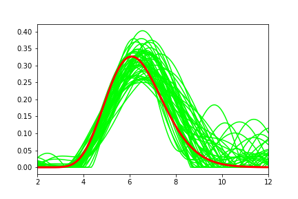
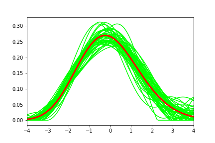
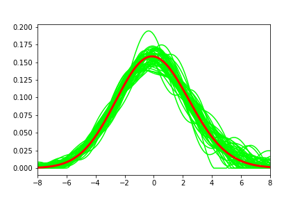
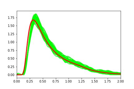
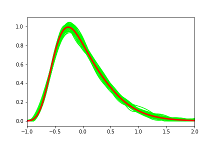
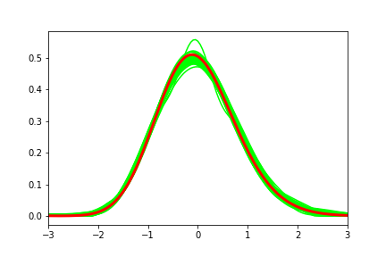
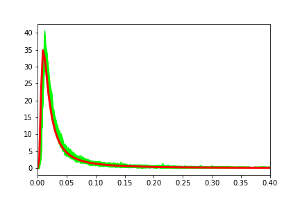
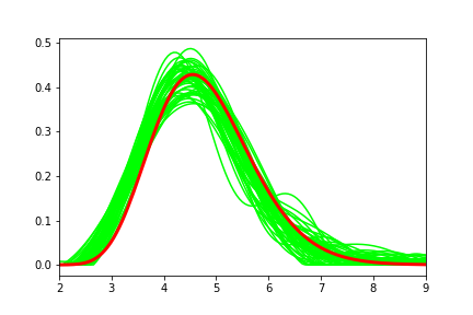
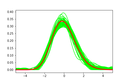
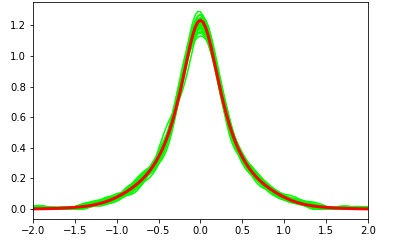
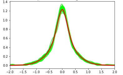
Figure 1 illustrates the behaviour of our procedure for $\alpha$-stable processes, while Figure 2 demonstrates it for tempered stable processes, displaying the outcomes of 50 estimators. Tables 1 and 2 present the estimated relative $L^{2}$ risks, along with their standard deviations, for the symmetric and non-symmetric $\alpha$-stable cases, respectively. Additionally, Table 3 provides the same metrics for the tempered case. These estimations are obtained via Monte Carlo simulation over 100 iterations. The tables also include the mean and standard deviation of the selected $\widehat{m}$ values.

A preliminary observation is that, as expected, we observe improvements in both the graphs and the risks as $n$ increases. Below we discuss the influence of $\alpha$ and $\Delta$. We recall that the rate is provided in (10), which increases as $\Delta$ decreases and increases as $\alpha$ deceases.

Discussion on the influence of $\alpha$

Given $n$ and $\Delta$ we observe in Tables 1 and 2 that indeed the relative $L^{2}$ error decreases with $\alpha$. The estimator is more accurate when the jump activity is higher. This phenomenon can be interpreted in various ways. In the case of high frequency observations, the fact that better results are obtained as $\alpha$ increases can be explained by the observation that as $\alpha$ becomes larger, $\|f_{\Delta}-g_{\Delta}\|^{2}$ gets smaller. For instance, using similar arguments as those employed in the proof of Theorem 2, one can show that $\|f_{\Delta}-g_{\Delta}\|^{2}\leq e^{2\lambda\Delta}\frac{\Gamma(1/\alpha)}{(2\alpha M)^{\frac{1}{\alpha}}}\Delta^{2-\frac{1}{\alpha}}$. Consequently, as $\alpha$ increases, the inverse problem starts resembling more and more a direct problem, yielding more informative observations for the estimation of $g_{\Delta}$. In the scenario where $\Delta$ is fixed, this phenomenon can be attributed to the fact that in such a regime the Gaussian approximation of small jumps is better, and the approximation improves as $\alpha$ increases, see e.g. Theorem 1 in [11]. With increasing $\alpha$, we move closer to a parametric problem, implying a potential improvement in convergence rates.

Moreover in both Figures 1 and 2 we notice that the larger $\alpha$, the larger the support of $g_{\Delta}$ gets. When $\alpha$ gets close to 2 the estimated curve is visually similar to the density of a Gaussian random variable. Finally, we observe that the supremum of $g_{\Delta}$ decreases with $\alpha$, which is consistent with the behavior in $\alpha$ of the bound given in Lemma 2 which allows to derive

$\displaystyle\|{g_{\Delta}}\|_{\infty}\leq\tfrac{1}{2\varepsilon}+\tfrac{1}{\alpha}\tfrac{\pi}{2(\Delta M)^{\frac{1}{\alpha}}}\Gamma\left(\tfrac{1}{\alpha},\frac{\Delta M}{\varepsilon^{\alpha}}\right).$ (22)

Discussion on the influence of $\Delta$

In Tables 1 and 2, as well as in Figure 1, the risks appear to be smaller for $\Delta=0.1$ than when $\Delta=1$ or $\Delta=0.01$. This might seem surprising, given that in (10), the rate seems to be smaller for larger values of $\Delta$. However, this observation is valid only when we neglect the quantity $e^{4\lambda\Delta}$. When we take this into account, we notice that the $L^{2}$ bound is indeed smaller for $\Delta=0.1$ compared to both $\Delta=0.01$ and $\Delta=1$, which is consistent with what is observed in Tables 1 and 2. Additionally, note that Figure 1 illustrates that as $\Delta$ decreases, the estimated $\|\widehat{g}_{\Delta,\widehat{m}}\|_{\infty}$ increases, accordingly to the bound provided in (22).

Comparison between $\alpha$-stable and tempered stable Lévy processes

The comparison of Table 3 with Table 2 for $\Delta=1$ reveals better performances of the estimator in the tempered stable case compared to the $\alpha$-stable one. Due to computational time limitations the case $\alpha=1.7$ is not considered in Table 3. Heuristically, one of the distinctive characteristics of tempered stable processes is the reduced concentration of mass on big jumps, due to the exponential term in the Lévy measure. This means that we are more likely to observe small jumps in comparison to the $\alpha$-stable case. Consequently, it was expected that the estimator would exhibit better performances in the tempered setting. This is emphasized in the case where $\Delta=1$ where the compensation of big jumps complicates the distinction between small and large jumps.

3.3 Estimation in presence of a Brownian part

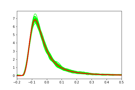
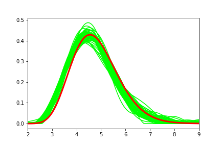
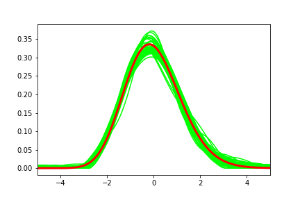
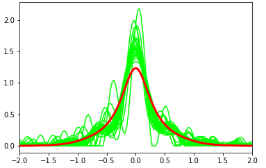
Finally, we illustrate how the presence of a Gaussian component affects the numerical results. We demonstrate this phenomenon by perturbing the same $1$-stable Lévy process with the addition of a Brownian part $\sigma B$ for different values of $\sigma$. We observe in Table 4 and Figure 3 that the relative $L^{2}$ error deteriorates as $\sigma$ increases, as noted in Theorem 5 and Corollary 2.

$\sigma=0$ $\sigma=0.2$ $\sigma=0.5$ $\sigma=1$
$\tfrac{\lVert\widehat{g}_{\Delta,\widehat{m}}-g_{\Delta}\rVert^{2}}{\lVert g_{\Delta}\rVert^{2}}$ $\overline{\widehat{m}}$ $\tfrac{\lVert\widehat{g}_{\Delta,\widehat{m}}-g_{\Delta}\rVert^{2}}{\lVert g_{\Delta}\rVert^{2}}$ $\overline{\widehat{m}}$ $\tfrac{\lVert\widehat{g}_{\Delta,\widehat{m}}-g_{\Delta}\rVert^{2}}{\lVert g_{\Delta}\rVert^{2}}$ $\overline{\widehat{m}}$ $\tfrac{\lVert\widehat{g}_{\Delta,\widehat{m}}-g_{\Delta}\rVert^{2}}{\lVert g_{\Delta}\rVert^{2}}$ $\overline{\widehat{m}}$
$1.72\times 10^{-2}$ 1.597 $1.91\times 10^{-2}$ 1.596 $2.11\times 10^{-2}$ 1.582 $9.97\times 10^{-2}$ 1.589
(0.016) (0.08) (0.022) (0.08) (0.020) (0.04) (0.12) (0.06)
Table 4: Mean and standard deviation of the estimated relative $L^{2}$ risk and selected cut-off $\widehat{m}$ from 100 estimators for $n=5000$, $\alpha=1$ $P=1,Q=1,A=0$.
Refer to caption
Refer to caption
Refer to caption
Figure 3: Plot of $30$ of realizations of $\widehat{g}_{\Delta,\widehat{m}}$ (green) using the same symmetric $1-$stable process (with $P=1,Q=1,A=0$) perturbed by a Brownian motion with $\sigma\in\{0,0.2,0.5\}$ and an approximation of $g_{\Delta}$ (red) by Fourier inversion with $\Delta=0.1$, $n=5000$.

4 Proofs

4.1 Proof of Theorem 2

To control the integrated $L^{2}$-risk introduce the notation $f_{\Delta,m}$, the uniquely defined function with Fourier transform $\mathcal{F}f_{\Delta,m}=(\mathcal{F}f_{\Delta})\mathds{1}_{[-m,m]}$, where $f_{\Delta}$ is the density of the whole increment $X_{\Delta}$. We write the decomposition

$\displaystyle\mathbb{E}[\|\widetilde{g}_{\Delta,m}-g_{\Delta}\|^{2}]=\|f_{\Delta,m}-g_{\Delta}\|^{2}+\frac{1}{2\pi}\int_{-m}^{m}\mathbb{E}[|\widehat{\phi}_{X_{\Delta}}(u)-\phi_{X_{\Delta}}(u)|^{2}]du.$

The second variance term is easily bounded as in the proof of Theorem 1 by $\frac{e^{4}m}{\pi n}$, under the assumption $\lambda\Delta\leq 1$. The first term is a bias term for which we can write

$\displaystyle\|f_{\Delta,m}-g_{\Delta}\|^{2}$ $\displaystyle\leq 2\|f_{\Delta,m}-g_{\Delta,m}\|^{2}+2\|g_{\Delta,m}-g_{\Delta}\|^{2}.$

An upper bound for $\|g_{\Delta,m}-g_{\Delta}\|^{2}$ is provided in (8). By means of Plancherel’s equality and (5), it holds:

$\displaystyle\|f_{\Delta,m}-g_{\Delta,m}\|^{2}$ $\displaystyle=\frac{1}{2\pi}\int_{[-m,m]}|\phi_{X_{\Delta}}(u)|^{2}\left|1-\frac{1}{\phi_{X^{B}_{\Delta}}(u)}\right|^{2}du.$

Recalling that $(\phi_{X_{\Delta}^{B}}(u))^{-1}=e^{\lambda\Delta(1-\phi_{Y_{1}}(u))}$, by means of the mean value theorem we get

$$\bigg{|}1-\frac{1}{\phi_{X_{\Delta}^{B}}(u)}\bigg{|}\leq e^{2\lambda\Delta}-1\leq 2\lambda\Delta e^{2\lambda\Delta}\leq 2\lambda\Delta e^{2}.$$

Hence,

$\displaystyle\|f_{\Delta,m}-g_{\Delta,m}\|^{2}$ $\displaystyle\leq\frac{2e^{4}(\lambda\Delta)^{2}}{\pi}\int_{\mathbb{R}}|\phi_{X_{\Delta}}(u)|^{2}du.$

Furthermore, using (38) in Lemma 2 and the inequality $\Gamma(s,x)\leq 2^{s}e^{-x/2}\Gamma(s)$ for $s,x>0$, we obtain

$\displaystyle\|\phi_{X_{\Delta}}\|_{2}^{2}$ $\displaystyle\leq\int_{|u|\geq\frac{\pi}{2\varepsilon}}|\phi_{X_{\Delta}}(u)|^{2}du+\int_{|u|\leq\frac{\pi}{2\varepsilon}}|\phi_{X_{\Delta}}(u)|^{2}du\leq 2\int_{\frac{\pi}{2\varepsilon}}^{\infty}e^{-\frac{2^{\alpha+1}M}{\pi^{\alpha}}u^{\alpha}\Delta}du+\frac{\pi}{\varepsilon}$
$\displaystyle=\Delta^{-\frac{1}{\alpha}}\frac{\pi}{2^{1+\frac{1}{\alpha}}\alpha M^{\frac{1}{\alpha}}}\Gamma\left(\frac{1}{\alpha},\frac{2M\Delta}{\varepsilon^{\alpha}}\right)+\frac{\pi}{\varepsilon}\leq\Delta^{-\frac{1}{\alpha}}\frac{\pi}{2^{1+\frac{1}{\alpha}}\alpha M^{\frac{1}{\alpha}}}e^{-\frac{M\Delta}{2\varepsilon^{\alpha}}}2^{\frac{1}{\alpha}}\Gamma(\tfrac{1}{\alpha})+\frac{\pi}{\varepsilon}$
$\displaystyle\leq K^{\prime}\left(\Delta^{-\frac{1}{\alpha}}e^{-\kappa\frac{\Delta}{\varepsilon^{\alpha}}}+\tfrac{1}{\varepsilon}\right),$

for some positive constants $K^{\prime},\,\kappa$, depending on $\alpha$ and $M$. Gathering both terms we derive that there exist two positive constants $K$ and $\kappa$ such that

$\displaystyle\|f_{\Delta,m}-g_{\Delta,m}\|^{2}$ $\displaystyle\leq K\lambda^{2}\left(\Delta^{2-\frac{1}{\alpha}}e^{-\kappa\frac{\Delta}{\varepsilon^{\alpha}}}+\Delta^{2}\varepsilon^{-1}\right).$ (23)

Collecting all terms, we derive the desired result.

4.2 Proof of Theorem 3

The proof is divided in four steps described before Theorem 3.

Step 1: We begin by showing that

$$\inf_{\widehat{g}_{\Delta}}\sup_{g_{\Delta}\in\mathcal{A}_{M,\alpha_{0}}}\mathbb{E}\|\widehat{g}_{\Delta}-g_{\Delta}\|^{2}\geq\inf_{\widehat{f}_{\Delta}}\sup_{f_{\Delta}\in{\mathcal{S}}_{\alpha_{0}}}\mathbb{E}\|\widehat{f}_{\Delta}-f_{\Delta}\|^{2},$$

where $\mathcal{S}_{\alpha_{0}}$ denotes the class of symmetric $\alpha$-stable densities with $\alpha\in[\alpha_{0},2)$ and with characteristic function $e^{-\Delta|u|^{\alpha}}$ and the second infimum is taken over all possible estimators $\widehat{f}_{\Delta}$ of the density $f_{\Delta}$ of $X_{\Delta}$. It is the marginal of a symmetric $\alpha$-stable process, for $\alpha\in[\alpha_{0},2)$, if $f_{\Delta}\in{\mathcal{S}}_{\alpha_{0}}$.

Let $\mu=\delta_{0}+{\rm Leb}$ and denote by $\mathcal{F_{\mu}}$ the set of densities with respect to the measure $\mu$. Recall that $f_{\Delta}$ stands for the density of the law of $X_{\Delta}$ with respect to the Lebesgue measure and by $h_{\Delta}$ that of the law of $X_{\Delta}^{B}$ with respect to $\mu$. We make two observations: first $\|h_{\Delta}\|_{1,\mu}=\int h_{\Delta}(x)\mu(dx)=1\geq\|h_{\Delta}\|_{1}$ and second the Young inequality allows to write that $\|g\star h\|_{2}\leq\|g\|_{2}\|h\|_{1}$ for $g\in L_{2}$ and $h\in L_{1}$. Consequently, we derive that

$\displaystyle\inf_{\widehat{g}_{\Delta}}\sup_{g_{\Delta}\in\mathcal{A}_{M,\alpha_{0}}}\mathbb{E}\|\widehat{g}_{\Delta}-g_{\Delta}\|^{2}$ $\displaystyle=\inf_{\widehat{g}_{\Delta}}\sup_{g_{\Delta}\in\mathcal{A}_{M,\alpha_{0}}}\sup_{h_{\Delta}\in\mathcal{F}_{\mu}}\mathbb{E}\|\widehat{g}_{\Delta}-g_{\Delta}\|^{2}\|h_{\Delta}\|_{1,\mu}^{2}$
$\displaystyle\geq\inf_{\widehat{g}_{\Delta}}\sup_{g_{\Delta}\in\mathcal{A}_{M,\alpha_{0}}}\sup_{h_{\Delta}\in\mathcal{F}_{\mu}}\mathbb{E}\|\widehat{g}_{\Delta}\star h_{\Delta}-g_{\Delta}\star h_{\Delta}\|^{2}$
$\displaystyle=\inf_{\widehat{g}_{\Delta}}\sup_{{f_{\Delta},f_{\Delta}=g_{\Delta}\star h_{\Delta}}\atop{g_{\Delta\in\mathcal{A}_{M,\alpha_{0}},\,h_{\Delta}\in\mathcal{F}_{\mu}}}}\mathbb{E}\|\widehat{g}_{\Delta}\star h_{\Delta}-f_{\Delta}\|^{2}$
$\displaystyle\geq\inf_{\widehat{f}_{\Delta}}\sup_{f_{\Delta}\in{\mathcal{S}}_{\alpha_{0}}}\mathbb{E}\|\widehat{f}_{\Delta}-f_{\Delta}\|^{2},$

where we used that if $f_{\Delta}\in\mathcal{S}_{\alpha_{0}}$ then for

$\displaystyle M\leq F(\alpha_{0}):=\begin{cases}\left(\frac{2-\alpha_{0}}{\alpha_{0}}\cos(\frac{\pi\alpha_{0}}{2})\Gamma({1-\alpha_{0}})\right)^{-1}&\text{if }\alpha_{0}\neq 1,\\ \frac{2}{\pi}&\text{if }\alpha_{0}=1,\\ \end{cases}$ (24)

there exists $g_{\Delta}\in\mathcal{A}_{M,\alpha_{0}}$ and $h_{\Delta}\in\mathcal{F}_{\mu}$ such that $f_{\Delta}=g_{\Delta}\star h_{\Delta}$. Indeed, if $f_{\Delta}$ is the marginal density of $X_{\Delta}\sim S_{\alpha_{0}}(\Delta^{\frac{1}{\alpha_{0}}},0,0)$ its characteristic function is $e^{-\Delta|u|^{\alpha_{0}}}$ and is associated with the Lévy density $p(x)=\frac{P}{|x|^{1+\alpha_{0}}}\mathbf{1}_{x\neq 0}$ where $P=\left(2\cos\left(\frac{\pi\alpha_{0}}{2}\right)\alpha_{0}^{-1}\Gamma(1-\alpha_{0})\right)^{-1}$ ([3] p.215) for which it holds that for all $\eta\in[-\epsilon,\epsilon]$ $\int_{[-\eta,\eta]}x^{2}p(x)dx=P^{-1}\eta^{2-\alpha_{0}}\geq M\eta^{2-\alpha_{0}}$, then $g_{\Delta}\in\mathcal{A}_{M,\alpha_{0}}$.

Step 2: Denote by

$\displaystyle\mathcal{R}_{\alpha_{0}}$ $\displaystyle:=\bigg{\{}\phi_{\Delta}:\mathbb{R}\to\mathbb{R}:\exists\beta\in[\alpha_{0},2)\ \text{such that }\phi_{\Delta}(t)=e^{-\Delta|t|^{\beta}},\forall t\in\mathbb{R}\bigg{\}},$
$\displaystyle\widetilde{\mathcal{R}}_{\alpha_{0}}$ $\displaystyle:=\bigg{\{}\phi_{\Delta}:\exists\beta\in\Big{[}\alpha_{0},\alpha_{0}-\frac{2}{\log(\Delta)}\Big{]}\subset(0,2)\ \text{such that }\phi_{\Delta}(t)=e^{-\Delta|t|^{\beta}},\forall t\in\mathbb{R}\bigg{\}}$

and observe that $\widetilde{\mathcal{R}}_{\alpha_{0}}\subseteq{\mathcal{R}}_{\alpha_{0}}$, since $\Delta<e^{-\frac{2}{2-\alpha_{0}}}$. Thus, using Plancherel equality we write, if we set $\phi_{\alpha,\Delta}(t):=e^{-\Delta|t|^{\alpha}},\ t\in\mathbb{R}$,

$\displaystyle\inf_{\widehat{f}_{\Delta}}\sup_{f_{\Delta}\in\mathcal{S}_{\alpha_{0}}}\mathbb{E}\|\widehat{f}_{\Delta}-f_{\Delta}\|^{2}$ $\displaystyle=\frac{1}{2\pi}\inf_{\widehat{\phi}_{\Delta}}\sup_{\phi_{\Delta}\in\mathcal{R}_{\alpha_{0}}}\mathbb{E}\|\widehat{\phi}_{\Delta}-\phi_{\Delta}\|^{2}\geq\frac{1}{2\pi}\inf_{\widehat{\phi}_{\Delta}}\sup_{\phi_{\alpha,\Delta}\in\widetilde{\mathcal{R}}_{\alpha_{0}}}\mathbb{E}\|\widehat{\phi}_{\Delta}-\phi_{\alpha,\Delta}\|^{2}.$

Next, we show that we can focus on estimators of the parameter $\alpha$ to estimate $\phi_{\alpha,\Delta}$. For a given estimator $\widehat{\phi}_{\Delta}$ we define the quantity

$$\widehat{\alpha}(\widehat{\phi}_{\Delta})\in\mbox{arg}\min_{\alpha\in[\alpha_{0},\alpha_{0}+\frac{2}{\log(1/\Delta)}]}\mathbb{E}\|\widehat{\phi}_{\Delta}-\phi_{\alpha,\Delta}\|^{2}.$$

It follows that $\phi_{\widehat{\alpha}(\widehat{\phi}_{\Delta}),\Delta}$ is the characteristic function of the symmetric stable process in $\widetilde{\mathcal{R}}_{\alpha_{0}}$ closest to the estimator $\widehat{\phi}_{\Delta}$. This allows to deduce that for all $\alpha\in[\alpha_{0},\alpha_{0}+\frac{2}{\log(1/\Delta)}]$ and for all estimator $\widehat{\phi}_{\Delta}$

$\displaystyle\mathbb{E}\|\phi_{\widehat{\alpha}(\widehat{\phi}_{\Delta}),\Delta}-\phi_{\alpha,\Delta}\|^{2}$ $\displaystyle\leq 2\mathbb{E}\|\phi_{\widehat{\alpha}(\widehat{\phi}_{\Delta}),\Delta}-\widehat{\phi}_{\Delta}\|^{2}+2\mathbb{E}\|\widehat{\phi}_{{\Delta}}-\phi_{\alpha,\Delta}\|^{2}\leq 4\mathbb{E}\|\widehat{\phi}_{{\Delta}}-\phi_{\alpha,\Delta}\|^{2}.$

Injecting this in the latter inequality we derive

$\displaystyle\inf_{\widehat{f}_{\Delta}}\sup_{f_{\Delta}\in\mathcal{S}_{\alpha_{0}}}\mathbb{E}\|\widehat{f}_{\Delta}-f_{\Delta}\|^{2}$ $\displaystyle\geq\frac{1}{8\pi}\inf_{\widehat{\phi}_{\Delta}}\sup_{\phi_{\alpha,\Delta}\in{\widetilde{\mathcal{R}}_{\alpha_{0}}}}\mathbb{E}\|\phi_{\widehat{\alpha}(\widehat{\phi}_{\Delta}),\Delta}-\phi_{\alpha,\Delta}\|^{2}$
$\displaystyle\geq\frac{1}{8\pi}\inf_{\widehat{\alpha}\in[0,2]}\sup_{{\alpha}\in[\alpha_{0},\alpha_{0}+\frac{2}{\log(1/\Delta)}]}\mathbb{E}\|\phi_{\widehat{\alpha},\Delta}-\phi_{\alpha,\Delta}\|^{2}.$

Step 3: In this step, we control the quantity $\mathbb{E}\|\phi_{\widehat{\alpha},\Delta}-\phi_{\alpha,\Delta}\|^{2}$. For that we introduce the event

$$A_{\widehat{\alpha},\alpha_{0}}=\Big{\{}\omega\in\Omega:\log(1/\Delta)|\widehat{\alpha}(\omega)-\alpha_{0}|\leq 2\Big{\}}$$

and the quantities

$$m_{\alpha}:=\min(\alpha,\widehat{\alpha})\geq 0,\quad M_{\alpha}:=\max(\alpha,\widehat{\alpha})\leq 2.$$

The step is divided in three points, where we control $\mathbb{E}\|\phi_{\widehat{\alpha},\Delta}-\phi_{\alpha,\Delta}\|^{2}$ respectively on $A_{\widehat{\alpha},\alpha_{0}}$, $A_{\widehat{\alpha},\alpha_{0}}^{c}$ before concluding.

Step 3.1: We first restrict to the event $A_{\widehat{\alpha},\alpha_{0}}$ and $\alpha\in[\alpha_{0},\alpha_{0}+\frac{2}{\log(1/\Delta)}]$. By Lagrange theorem applied to the function $h(x)=e^{-\Delta u^{x}}$, for any $\omega\in A_{\widehat{\alpha},\alpha_{0}}$ there exists $\xi\in[m_{\alpha}(\omega),M_{\alpha}(\omega)]$ such that

$\displaystyle\Big{(}e^{-\Delta u^{m_{\alpha}(\omega)}}-e^{-\Delta u^{M_{\alpha}(\omega)}}\Big{)}^{2}$ $\displaystyle=|\widehat{\alpha}(\omega)-\alpha|^{2}\Delta^{2}e^{-2\Delta u^{\xi}}u^{2\xi}\log^{2}(u)$
$\displaystyle\geq\frac{|\widehat{\alpha}(\omega)-\alpha|^{2}\Delta^{2}}{M_{\alpha}^{2}(\omega)}\log^{2}(\Delta)e^{-2\Delta u^{M_{\alpha}(\omega)}}u^{2m_{\alpha}(\omega)},$

for all $u\geq\Delta^{-\frac{1}{M_{\alpha}(\omega)}}$. Using that $M_{\alpha}\leq 2$, $m_{\alpha}\geq 0$ and $\frac{2m_{\alpha}+1}{M_{\alpha}}\leq\frac{2\alpha+1}{\alpha}$ we derive

$\displaystyle\mathbb{E}\big{[}\|\phi_{\widehat{\alpha},\Delta}-\phi_{\alpha,\Delta}\|^{2}\mathbf{1}_{A_{\widehat{\alpha},\alpha_{0}}}\big{]}$ $\displaystyle=2\int_{0}^{\infty}\mathbb{E}\bigg{[}\mathbf{1}_{A_{\widehat{\alpha},\alpha_{0}}}\Big{(}e^{-\Delta u^{m_{\alpha}}}-e^{-\Delta u^{M_{\alpha}}}\Big{)}^{2}\bigg{]}du$
$\displaystyle\geq 2\mathbb{E}\bigg{[}\mathbf{1}_{A_{\widehat{\alpha},\alpha_{0}}}\int_{\frac{1}{\Delta^{1/{M_{\alpha}}}}}^{\infty}\frac{|\widehat{\alpha}-\alpha|^{2}\Delta^{2}}{4}\log^{2}(\Delta)e^{-2\Delta u^{M_{\alpha}}}u^{2m_{\alpha}}du\bigg{]}$
$\displaystyle\geq\frac{1}{2}\log^{2}(\Delta)\mathbb{E}\bigg{[}\mathbf{1}_{A_{\widehat{\alpha},\alpha_{0}}}|\widehat{\alpha}-\alpha|^{2}\Delta^{2}\frac{\Gamma\Big{(}\frac{2m_{\alpha}+1}{M_{\alpha}},2\Big{)}}{M_{\alpha}}\big{(}2\Delta\big{)}^{-\frac{2m_{\alpha}+1}{M_{\alpha}}}\bigg{]}$
$\displaystyle\geq\frac{2^{-\frac{2\alpha+1}{\alpha}}}{4}\log^{2}(\Delta)\mathbb{E}\bigg{[}\mathbf{1}_{A_{\widehat{\alpha},\alpha_{0}}}|\widehat{\alpha}-\alpha|^{2}\Delta^{\frac{2(M_{\alpha}-m_{\alpha})-1}{M_{\alpha}}}\Gamma\Big{(}\frac{2m_{\alpha}+1}{M_{\alpha}},2\Big{)}\bigg{]}$
$\displaystyle\geq\frac{2^{-\frac{2\alpha+1}{\alpha}}\int_{2}^{\infty}\frac{e^{-t}}{\sqrt{t}}dt}{4}\log^{2}(\Delta)\mathbb{E}\bigg{[}\mathbf{1}_{A_{\widehat{\alpha},\alpha_{0}}}|\widehat{\alpha}-\alpha|^{2}\Delta^{\frac{2(M_{\alpha}-m_{\alpha})-1}{M_{\alpha}}}\bigg{]}.$ (25)

We write $\Delta^{\frac{2(M_{\alpha}-m_{\alpha})-1}{M_{\alpha}}}=\Delta^{\frac{2(M_{\alpha}-m_{\alpha})}{M_{\alpha}}}\Delta^{-\frac{1}{\alpha_{0}}+\frac{M_{\alpha}(\omega)-\alpha_{0}}{\alpha_{0}M_{\alpha}(\omega)}}$ and we notice that for any $\omega\in A_{\widehat{\alpha},\alpha_{0}}$ and $\alpha\in[\alpha_{0},\alpha_{0}+\frac{2}{\log(1/\Delta)}]$, it holds:

$\displaystyle\frac{M_{\alpha}(\omega)-\alpha_{0}}{\alpha_{0}M_{\alpha}(\omega)}$ $\displaystyle\leq\frac{|\widehat{\alpha}(\omega)-\alpha_{0}|+|\alpha-\alpha_{0}|}{\alpha\alpha_{0}}\leq\frac{4}{\alpha_{0}^{2}\log(1/\Delta)},$
$\displaystyle\frac{M_{\alpha}(\omega)-m_{\alpha}(\omega)}{M_{\alpha}(\omega)}$ $\displaystyle=\frac{|\widehat{\alpha}(\omega)-\alpha|}{M_{\alpha}(\omega)}\leq\frac{4}{\alpha_{0}\log(1/\Delta)}.$

Hence, from the previous inequalities, we derive

$\displaystyle\Delta^{\frac{2(M_{\alpha}-m_{\alpha})-1}{M_{\alpha}}}\geq\Delta^{-\frac{1}{\alpha_{0}}}\Delta^{\frac{4}{\alpha_{0}\log(1/\Delta)}\big{(}2+\frac{1}{\alpha_{0}}\big{)}}=\Delta^{-\frac{1}{\alpha_{0}}}e^{-\frac{4}{\alpha_{0}}\big{(}2+\frac{1}{\alpha_{0}}\big{)}}.$ (26)

Moreover, we observe that

$\displaystyle\sup_{\alpha\in[\alpha_{0},\alpha_{0}+\frac{2}{\log(1/\Delta)}]}2^{-\frac{2\alpha+1}{\alpha}}\geq 2^{-\big{(}\frac{1}{\alpha_{0}}+2\big{)}}.$ (27)

Injecting (26) and (27) in (25) we deduce that

$\displaystyle\sup_{\alpha\in[\alpha_{0},\alpha_{0}+\frac{2}{\log(1/\Delta)}]}\mathbb{E}\big{[}\|\phi_{\widehat{\alpha},\Delta}-\phi_{\alpha,\Delta}\|^{2}\mathbf{1}_{A_{\widehat{\alpha},\alpha_{0}}}\big{]}\geq\frac{C_{0}}{n\Delta^{\frac{1}{\alpha_{0}}}}\sup_{\alpha\in[\alpha_{0},\alpha_{0}+\frac{2}{\log(1/\Delta)}]}\mathbb{E}\big{[}\mathbf{1}_{A_{\widehat{\alpha},\alpha_{0}}}n\log^{2}(\Delta)|\widehat{\alpha}-\alpha|^{2}\Big{]}$

where $C_{0}$ is a positive constant only depending on $\alpha_{0}$ defined as follows:

$\displaystyle C_{0}=\frac{2^{-\frac{1}{\alpha_{0}}}e^{-\frac{4}{\alpha_{0}}\big{(}2+\frac{1}{\alpha_{0}}\big{)}}\int_{2}^{\infty}\frac{e^{-t}}{\sqrt{t}}dt}{16}.$ (28)

Step 3.2: We now restrict to the event $A^{c}_{\widehat{\alpha},\alpha_{0}}$ and $\alpha\in[\alpha_{0},\alpha_{0}+\frac{2}{\log(1/\Delta)}]$. Let $\omega\in A^{c}_{\widehat{\alpha},\alpha_{0}}$ and $u\geq\Delta^{-\frac{1}{m_{\alpha}(\omega)}}$, we justify that $e^{-\Delta u^{m_{\alpha}(\omega)}}-e^{-\Delta u^{M_{\alpha}(\omega)}}\geq\frac{e^{-\Delta u^{m_{\alpha}(\omega)}}}{2}$. Indeed, using that $m_{\alpha}\leq 2$ we write

$\displaystyle u^{M_{\alpha}(\omega)}-u^{m_{\alpha}(\omega)}$ $\displaystyle=u^{m_{\alpha}(\omega)}\Big{(}u^{|\widehat{\alpha}(\omega)-\alpha|}-1\Big{)}\geq\frac{1}{\Delta}\bigg{(}\Delta^{\frac{2}{m_{\alpha}(\omega)\log(\Delta)}}-1\bigg{)}$
$\displaystyle=\frac{e^{\frac{2}{m_{\alpha}(\omega)}}-1}{\Delta}\geq\frac{2}{\Delta m_{\alpha}(\omega)}\geq\frac{1}{\Delta}\geq\frac{\log 2}{\Delta},$

which implies that $e^{\Delta(u^{M_{\alpha}(\omega)}-u^{m_{\alpha}(\omega)})}\geq 2$ and the desired inequality. As a consequence, we get

$\displaystyle\mathbb{E}\big{[}\|\phi_{\widehat{\alpha},\Delta}-\phi_{\alpha,\Delta}\|^{2}\mathbf{1}_{A^{c}_{\widehat{\alpha},\alpha_{0}}}\big{]}$ $\displaystyle\geq\frac{1}{2}\mathbb{E}\bigg{[}\mathbf{1}_{A^{c}_{\widehat{\alpha},\alpha_{0}}}\int_{\Delta^{-1/m_{\alpha}}}^{2\Delta^{-1/m_{\alpha}}}e^{-2\Delta u^{m_{\alpha}}}du\bigg{]}$
$\displaystyle\geq\frac{1}{2}\mathbb{E}\bigg{[}\mathbf{1}_{A^{c}_{\widehat{\alpha},\alpha_{0}}}\Delta^{-\frac{1}{m_{\alpha}}}e^{-2^{1+m_{\alpha}}}\bigg{]}$
$\displaystyle\geq\frac{1}{2}\mathbb{E}\bigg{[}\mathbf{1}_{A^{c}_{\widehat{\alpha},\alpha_{0}}}\Delta^{-\frac{1}{\alpha_{0}}}\Delta^{\frac{m_{\alpha}-\alpha_{0}}{\alpha_{0}m_{\alpha}}}e^{-8}\bigg{]}.$ (29)

In order to control the term $\Delta^{\frac{m_{\alpha}-\alpha_{0}}{\alpha_{0}m_{\alpha}}}$ we notice that for $\alpha\in[\alpha_{0},\alpha_{0}-\frac{2}{\log(\Delta)}]$ and $\omega\in A^{c}_{\widehat{\alpha},\alpha_{0}}$ it holds

$$\Delta^{\frac{m_{\alpha}-\alpha_{0}}{\alpha_{0}m_{\alpha}}}\geq\begin{cases}1&\text{ if }\quad m_{\alpha}(\omega)-\alpha_{0}\leq 0,\\ \Delta^{\frac{2}{\log(1/\Delta)\alpha_{0}^{2}}}=e^{-\frac{2}{\alpha_{0}^{2}}}&\text{ otherwise},\end{cases}$$

that is

$\displaystyle\Delta^{\frac{m_{\alpha}-\alpha_{0}}{\alpha_{0}m_{\alpha}}}\geq e^{-\frac{2}{\alpha_{0}^{2}}}.$ (30)

Injecting (30) in (4.2) we derive

$$\sup_{\alpha\in[\alpha_{0},\alpha_{0}+\frac{2}{\log(1/\Delta)}]}\mathbb{E}\big{[}\|\phi_{\widehat{\alpha},\Delta}-\phi_{\alpha,\Delta}\|^{2}\mathbf{1}_{A^{c}_{\widehat{\alpha},\alpha_{0}}}\big{]}\geq\frac{e^{-8-\frac{2}{\alpha_{0}^{2}}}}{2}\Delta^{-1/\alpha_{0}}\mathbb{E}\big{[}\mathbf{1}_{A^{c}_{\widehat{\alpha},\alpha_{0}}}\big{]}.$$

Step 3.3: This step aims at showing that

$\displaystyle\inf_{\widehat{\alpha}\in[0,2]}\sup_{\alpha\in[\alpha_{0},\alpha_{0}+\frac{2}{\log(1/\Delta)}]}\mathbb{E}\big{[}\|\phi_{\widehat{\alpha},\Delta}-\phi_{\alpha,\Delta}\|^{2}\big{]}\geq\inf_{\widehat{\alpha}\in[0,2]}\sup_{\alpha\in[\alpha_{0},\alpha_{0}+\frac{2}{\log(1/\Delta)}]}\frac{K_{0}}{n\Delta^{1/\alpha_{0}}}\mathbb{E}[n\log^{2}(\Delta)|\widehat{\alpha}-\alpha|^{2}],$ (31)

for some $K_{0}>$ which depending only on $\alpha_{0}$. Denote by

$$h(\widehat{\alpha},\alpha_{0}):=\sup_{\alpha\in[\alpha_{0},\alpha_{0}+\frac{2}{\log(1/\Delta)}]}\mathbb{E}\Big{[}\mathbf{1}_{A_{\widehat{\alpha},\alpha_{0}}}n\log^{2}(\Delta)|\widehat{\alpha}-\alpha|^{2}+n\mathbf{1}_{A^{c}_{\widehat{\alpha},\alpha_{0}}}\Big{]}.$$

Steps 3.1 and 3.2 allows to write that

$\displaystyle\inf_{\widehat{\alpha}\in[0,2]}\sup_{\alpha\in[\alpha_{0},\alpha_{0}+\frac{2}{\log(1/\Delta)}]}\mathbb{E}\big{[}\|\phi_{\widehat{\alpha},\Delta}-\phi_{\alpha,\Delta}\|^{2}\big{]}$ $\displaystyle\geq\frac{K_{0}}{n\Delta^{1/\alpha_{0}}}\inf_{\widehat{\alpha}}h(\widehat{\alpha},\alpha_{0})$

for $K_{0}=\min\big{(}\frac{e^{-8-{2}/{\alpha_{0}^{2}}}}{2},C_{0}\big{)}$, with $C_{0}$ defined in (28). Now, for all estimator $\widehat{\alpha}$ of $\alpha$ we define the estimator $\widecheck{\alpha}$ as

$$\widecheck{\alpha}(\omega):=\begin{cases}\widehat{\alpha}(\omega),\quad\text{if }\omega\in A_{\widehat{\alpha},\alpha_{0}},\\ \alpha_{0}-\frac{1}{\log(\Delta)},\quad\text{if }\omega\in A^{c}_{\widehat{\alpha},\alpha_{0}}.\end{cases}$$

On the one hand, using that $A_{\widecheck{\alpha},\alpha_{0}}=\Omega$ by definition of $\widecheck{\alpha}$, we have

$$h(\widecheck{\alpha},\alpha_{0})=\sup_{\alpha\in[\alpha_{0},\alpha_{0}+\frac{2}{\log(1/\Delta)}]}\mathbb{E}[n\log^{2}(\Delta)|\widecheck{\alpha}-\alpha|^{2}].$$

On the other hand $h(\widecheck{\alpha},\alpha_{0})\leq h(\widehat{\alpha},\alpha_{0})$ as if $\omega\in A_{\widehat{\alpha},\alpha_{0}}$ then $\widehat{\alpha}(\omega)=\widecheck{\alpha}(\omega)$ and if $\omega\in A^{c}_{\widehat{\alpha},\alpha_{0}}$ then

$\displaystyle h(\widecheck{\alpha},\alpha_{0})$ $\displaystyle=\sup_{\alpha\in[\alpha_{0},\alpha_{0}+\frac{2}{\log(1/\Delta)}]}n\log^{2}(\Delta)\Big{|}\alpha_{0}-\frac{1}{\log(\Delta)}-\alpha\Big{|}^{2}\leq n=h(\widehat{\alpha},\alpha_{0}).$

This means that

$$\inf_{\widehat{\alpha}}h(\widehat{\alpha},\alpha_{0})=\inf_{\widehat{\alpha}:A_{\alpha_{0},\widehat{\alpha}}=\Omega}h(\widehat{\alpha},\alpha_{0}),$$

and thus Equation (31) holds true.

Step 4: The last step consists in proving that

$\displaystyle\inf_{\widehat{\alpha}\in[0,2]}\sup_{\alpha\in[\alpha_{0},\alpha_{0}+\frac{2}{\log(1/\Delta)}]}\frac{1}{n\Delta^{1/\alpha_{0}}}\mathbb{E}[n\log^{2}(\Delta)|\widehat{\alpha}-\alpha|^{2}]\geq\frac{c}{n\Delta^{1/\alpha_{0}}}$ (32)

for some positive constant $c$ and for $n\log^{2}(\Delta)$ large enough. To that aim, we use the general theory on minimax bounds for parametric estimators under the LAN condition developed in Ibragimov and Has’minskii [25]. Indeed, Masuda establishes in [3] Theorem 3.2 p.218 that the family of symmetric $\alpha_{0}$-stable processes satisfy the LAN condition with a Fisher information given by $r_{n,\Delta,\alpha_{0}}:=I_{\alpha_{0}}n\log^{2}(1/\Delta),$ where $I_{\alpha_{0}}$ is a finite positive constant only depending on the parameter $\alpha_{0}\in(0,2)$ (see Equations (3.5) and (3.6) therein). Equation (32) is a consequence of Theorem 12.1 p.162 in [25], which ensures that for $n\log^{2}(\Delta)$ large enough, for any $\delta>0$

$$\inf_{\widehat{\alpha}\in[0,2]}\sup_{|\alpha-\alpha_{0}|\leq\delta}\mathbb{E}[r_{n,\Delta,\alpha_{0}}|\widehat{\alpha}-\alpha|^{2}]\geq\widetilde{c}>0,$$

for some positive constant $\widetilde{c}$. In our case, the interval over which the supremum is taken is not symmetric but rather of the form $[\alpha_{0},\alpha_{0}-\frac{2}{\log(\Delta)}]$. Adapting the proof of the Theorem 12.1, the same conclusion holds true, for a different constant. The ingredient that ensures the validity of the proof is the fact that $\frac{r_{n,\Delta,\alpha_{0}}}{\delta^{2}}=I_{\alpha_{0}}n\to\infty$ as $n\to\infty$. Finally, observing that for $\Delta\leq e^{-\frac{4}{2-\alpha_{0}}}$ we have $[\alpha_{0},\alpha_{0}-\frac{2}{\log(\Delta)}]\subseteq[\alpha_{0},\frac{\alpha_{0}}{2}+1]$, we derive

$\displaystyle\inf_{\widehat{\alpha}\in[0,2]}\sup_{\alpha\in[\alpha_{0},\alpha_{0}-\frac{2}{\log(\Delta)}]}\frac{\mathbb{E}[n\log^{2}(\Delta)|\widehat{\alpha}-\alpha|^{2}]}{n\Delta^{1/\alpha_{0}}}$
$\displaystyle\quad\geq\inf_{\alpha\in[\alpha_{0},\frac{\alpha_{0}}{2}+1]}\frac{1}{I_{\alpha}}\inf_{\widehat{\alpha}\in[0,2]}\sup_{\alpha\in[\alpha_{0},\alpha_{0}-\frac{2}{\log(\Delta)}]}\mathbb{E}[r_{n,\Delta,\alpha_{0}}|\widehat{\alpha}-\alpha|^{2}]\geq\inf_{\alpha\in[\alpha_{0},\frac{\alpha_{0}}{2}+1]}\frac{1}{I_{\alpha}}\widetilde{c}.$ (33)

Recalling that $I_{\alpha}$ is finite for any $\alpha\in(0,2)$, hence it is bounded on $[\alpha_{0},\frac{\alpha_{0}}{2}+1]$, we derive (32) as desired. The proof is now complete.

4.3 Proof of Corollary 1

The first part of the proof is already contained in the proof of Theorem 3, specifically derived from equations (13), (14), and (4.2). The proof of the second part of the statement is a simplification of the proofs of Theorems 1 and 2. More precisely, by means of Lemma 2, for any $m\geq\frac{\pi}{2}$ we get

$\displaystyle\mathbb{E}\|\widehat{f}_{\Delta,m}-f_{\Delta}\|^{2}$ $\displaystyle\leq\|f_{\Delta,m}-f_{\Delta}\|^{2}+\mathbb{E}\|\widehat{f}_{\Delta,m}-f_{\Delta,m}\|^{2}$
$\displaystyle=\frac{1}{2\pi}\int_{[-m,m]^{c}}|\phi_{X_{\Delta}}(u)|^{2}du+\frac{1}{2\pi}\int_{-m}^{m}\mathbb{E}[|\widehat{\phi}_{X_{\Delta}}(u)-\phi_{X_{\Delta}}(u)|^{2}]du$
$\displaystyle\leq\frac{1}{\pi}\int_{m}^{\infty}e^{-\frac{2^{\alpha}M}{\pi^{\alpha}}u^{\alpha}\Delta}du+\frac{1}{2\pi}\int_{-m}^{m}\mathbb{V}\left(\frac{1}{n}\sum_{j=1}^{n}e^{iu(X_{j\Delta}-X_{(j-1)\Delta})}\right)du$
$\displaystyle\leq\frac{\Gamma\Big{(}\frac{1}{\alpha},\big{(}\frac{2m}{\pi}\big{)}^{\alpha}M\Delta\Big{)}}{2\alpha M^{\frac{1}{\alpha}}\Delta^{\frac{1}{\alpha}}}+\frac{m}{\pi n}.$

By derivation, we deduce that the choice of $m$ which minimizes the integrated $L_{2}$ risk is

$\displaystyle m^{\star}=\frac{\pi}{2M^{\frac{1}{\alpha}}\Delta^{\frac{1}{\alpha}}}\Big{(}\log\big{(}2M^{\frac{1}{\alpha}}\alpha n\Delta^{\frac{1}{\alpha}}\big{)}\Big{)}^{\frac{1}{\alpha}}.$

The proof is concluded by computing $\frac{m^{\star}}{\pi n}.$

4.4 Proof of Theorem 4

Firstly, we observe that

$$\gamma_{n}(\widehat{g}_{\Delta,\widehat{m}})+\mbox{pen}(\widehat{m})\leq\gamma_{n}(\widehat{g}_{\Delta,m})+\mbox{pen}(m).$$

Moreover

$\displaystyle\gamma_{n}(t)-\gamma_{n}(s)$ $\displaystyle=\|t-g_{\Delta}\|^{2}-\|s-g_{\Delta}\|^{2}-2\langle g_{\Delta},t-s\rangle-\frac{1}{\pi}\langle\widehat{\phi}_{Z_{\Delta}},\mathcal{F}(t-s)\rangle$
$\displaystyle=\|t-g_{\Delta}\|^{2}-\|s-g_{\Delta}\|^{2}-2\nu_{n}(t-s),$

where

$$\nu_{n}(t)=\frac{1}{2\pi}\langle\widehat{\phi}_{Z_{\Delta}}-\phi_{Z_{\Delta}},\mathcal{F}(t)\rangle=\frac{1}{2\pi n}\sum_{j=1}^{n}\int\left(\frac{e^{iu(X_{j\Delta}-X_{(j-1)\Delta})}}{\phi_{X^{B}_{\Delta}}(u)}-\frac{\mathbb{E}[e^{iuX_{\Delta}}]}{\phi_{X^{B}_{\Delta}}(u)}\right)\mathcal{F}t(-u)du,$$

using Plancherel. Combining these results, we derive

$\displaystyle\|\widehat{g}_{\Delta,\widehat{m}}-g_{\Delta}\|^{2}$ $\displaystyle\leq\|\widehat{g}_{\Delta,m}-g_{\Delta}\|^{2}+2\nu_{n}(\widehat{g}_{\Delta,\widehat{m}}-\widehat{g}_{\Delta,m})+\mbox{pen}(m)-\mbox{pen}(\widehat{m})$
$\displaystyle=\|\widehat{g}_{\Delta,m}-g_{\Delta}\|^{2}+2\|\widehat{g}_{\Delta,\widehat{m}}-\widehat{g}_{\Delta,m}\|\nu_{n}\left(\frac{\widehat{g}_{\Delta,\widehat{m}}-\widehat{g}_{\Delta,m}}{\|\widehat{g}_{\Delta,\widehat{m}}-\widehat{g}_{\Delta,m}\|}\right)+\mbox{pen}(m)-\mbox{pen}(\widehat{m})$
$\displaystyle\leq\|\widehat{g}_{\Delta,m}-g_{\Delta}\|^{2}+2\|\widehat{g}_{\Delta,\widehat{m}}-\widehat{g}_{\Delta,m}\|\sup_{t\in S_{m}+S_{\widehat{m}},\|t\|=1}\nu_{n}(t)+\mbox{pen}(m)-\mbox{pen}(\widehat{m})$
$\displaystyle\leq\|\widehat{g}_{\Delta,m}-g_{\Delta}\|^{2}+\frac{1}{4}\|\widehat{g}_{\Delta,\widehat{m}}-\widehat{g}_{\Delta,m}\|^{2}+4\sup_{t\in S_{m}+S_{\widehat{m}},\|t\|=1}\nu_{n}(t)^{2}+\mbox{pen}(m)-\mbox{pen}(\widehat{m})$
$\displaystyle\leq\frac{3}{2}\|\widehat{g}_{\Delta,m}-g_{\Delta}\|^{2}+\frac{1}{2}\|\widehat{g}_{\Delta,\widehat{m}}-g_{\Delta}\|^{2}+4\left(\sup_{t\in S_{m}+S_{\widehat{m}},\|t\|=1}\nu_{n}(t)^{2}-p(m,\widehat{m})\right)_{+}$
$\displaystyle\quad\quad+4p(m,\widehat{m})+\mbox{pen}(m)-\mbox{pen}(\widehat{m}),$

where $p(m,m^{\prime})=\frac{4}{\pi}e^{4\lambda\Delta}(m\vee m^{\prime})/n$ is fixed by applying the Talagrand inequality to $\nu_{n}$ (see the following Lemma 1). Note that $S_{m}+S_{m^{\prime}}=S_{m\vee m^{\prime}}.$

Lemma 1.

There exists a positive constant $C$ such that

$\displaystyle\mathbb{E}\left(\sup_{t\in{S_{m\vee\widehat{m}},\ \|t\|=1}}|\nu_{n}(t)|^{2}-4e^{4\lambda\Delta}\frac{m\vee\widehat{m}}{\pi n}\right)_{+}$ $\displaystyle\leq\frac{C}{n}.$

Plugging this result in above inequalities implies that

$\displaystyle\frac{1}{2}\mathbb{E}[\|\widehat{g}_{\Delta,\widehat{m}}-g_{\Delta}\|^{2}]$ $\displaystyle\leq\frac{3}{2}\left(\mathbb{E}[\|\widehat{g}_{\Delta,m}-g_{\Delta}\|^{2}]+\mbox{pen}(m)\right)+\frac{4C}{n}+\mathbb{E}[4p(m,\widehat{m})-\mbox{pen}(\widehat{m})]-\frac{1}{2}\mbox{pen}(m),$

using that for $\kappa>32/(3\pi)$

$$4p(m,\widehat{m})-\mbox{pen}(\widehat{m})-\frac{1}{2}\mbox{pen}(m)=\frac{e^{4\lambda\Delta}}{n}\left(\frac{16}{\pi}{(m\vee\widehat{m})}-\kappa\left(\frac{1}{2}m+\widehat{m}\right)\right)\leq 0.$$

The proof is completed by taking the infimum over $m$.

Proof of Lemma 1.

We apply the Talagrand inequality recalled in Lemma 3 in the Appendix. Note that we can write

$$\nu_{n}(t)=\frac{1}{n}\sum_{j=1}^{n}\big{(}f_{t}(X_{j\Delta}-X_{(j-1)\Delta})-\mathbb{E}[f_{t}(X_{\Delta})]\big{)}$$

where for $t\in S_{m\vee m^{\prime}}$,

$$f_{t}(x)=\frac{1}{2\pi}\int_{-m\vee m^{\prime}}^{m\vee m^{\prime}}\frac{e^{iux}}{\phi_{X^{B}_{\Delta}}(u)}\mathcal{F}t(-u)du.$$

For that we compute the three positive constants $M,\ H$ and $v$ introduced in Lemma 3. First note that as $\|t\|=1$ we get using Cauchy-Schwarz and (5) that

$\displaystyle\sup_{t\in S_{m\vee m^{\prime}},\|t\|=1}\|f_{t}\|_{\infty}\leq\left\|\frac{1}{\phi_{X^{B}_{\Delta}}}\right\|_{\infty}\frac{1}{2\pi}\sqrt{2(m\vee m^{\prime})}\sqrt{\int_{-m\vee m^{\prime}}^{m\vee m^{\prime}}|\mathcal{F}t(u)|^{2}du}\leq e^{2\lambda\Delta}\frac{\sqrt{m\vee m^{\prime}}}{\sqrt{\pi}}=:M.$

Using similar arguments we get

$\displaystyle\mathbb{E}\left(\sup_{t\in S_{m\vee m^{\prime}},\|t\|=1}|\nu_{n}({t})|\right)^{2}$ $\displaystyle\leq\mathbb{E}\left[\sup_{t\in S_{m\vee m^{\prime}},\|t\|=1}\nu_{n}({t})^{2}\right]\leq\frac{1}{2\pi}\int_{-m\vee m^{\prime}}^{m\vee m^{\prime}}\frac{\mathbb{E}[|\widehat{\phi}_{X_{\Delta}}(u)-\phi_{X_{\Delta}}(u)|^{2}]}{|\phi_{X^{B}_{\Delta}}(u)|^{2}}du$
$\displaystyle\leq\frac{e^{4\lambda\Delta}}{\pi n}(m\vee m^{\prime})=:H^{2}.$

Finally for the last term, following [15] we use the basis representation of the estimator to compute $v^{2}$. Indeed, using the basis (15) it holds $t=\sum_{j\in\mathbb{Z}}b_{j}\psi_{j,m\vee m^{\prime}}$ with $b_{j}=\langle t,\psi_{j,m\vee m^{\prime}}\rangle$ such that $\sum_{j\in\mathbb{Z}}b_{j}^{2}=1,$ and we can write

$\displaystyle\mathbb{V}(f_{t}(X_{\Delta}))$ $\displaystyle\leq\frac{1}{4\pi^{2}}\iint_{-m\vee m^{\prime}}^{m\vee m^{\prime}}\frac{\phi_{X_{\Delta}}(u-v)}{\phi_{X^{B}_{\Delta}}(u)\phi_{X^{B}_{\Delta}}(-v)}\mathcal{F}t(-u)\mathcal{F}t(v)dudv$
$\displaystyle=\frac{1}{4\pi^{2}}\sum_{j,k\in\mathbb{Z}}b_{j}b_{k}\iint_{-m\vee m^{\prime}}^{m\vee m^{\prime}}\frac{\phi_{X_{\Delta}}(u-v)}{\phi_{X^{B}_{\Delta}}(u)\phi_{X^{B}_{\Delta}}(-v)}\mathcal{F}\psi_{j,m\vee m^{\prime}}(-u)\mathcal{F}\psi_{k,m\vee m^{\prime}}(v)dudv$
$\displaystyle\leq\frac{1}{4\pi^{2}}\sqrt{\sum_{j,k\in\mathbb{Z}}b_{j}^{2}b_{k}^{2}\sum_{j,k\in\mathbb{Z}}\left|\iint_{-m\vee m^{\prime}}^{m\vee m^{\prime}}\frac{\phi_{X_{\Delta}}(u-v)}{\phi_{X^{B}_{\Delta}}(u)\phi_{X^{B}_{\Delta}}(-v)}\mathcal{F}\psi_{j,m\vee m^{\prime}}(-u)\mathcal{F}\psi_{k,m\vee m^{\prime}}(v)dudv\right|^{2}}$
$\displaystyle=\frac{1}{4\pi^{2}}\sqrt{\iint_{-m\vee m^{\prime}}^{m\vee m^{\prime}}\left|\frac{\phi_{X_{\Delta}}(u-v)}{\phi_{X^{B}_{\Delta}}(u)\phi_{X^{B}_{\Delta}}(-v)}\right|^{2}dudv}$
$\displaystyle\leq\frac{e^{4\lambda\Delta}}{4\pi^{2}}\sqrt{\iint_{-m\vee m^{\prime}}^{m\vee m^{\prime}}\left|{\phi_{X_{\Delta}}(u-v)}\right|^{2}dudv}\leq\frac{\sqrt{\pi}e^{4\lambda\Delta}}{2\pi^{2}}\sqrt{{m\vee m^{\prime}}}\|f_{X_{\Delta}}\|,$

where we used at the third line the Cauchy-Schwarz inequality on the index $\lambda=(j,k)$ and at the penultimate equality that for a bi-variate function $\phi(u,v)$ its norm can be computed as $\|\phi\|^{2}=\sum_{j,k\in\mathbb{Z}}\langle\phi,\psi_{j,m\vee m^{\prime}}\otimes\psi_{k,m\vee m^{\prime}}\rangle^{2}$. Therefore,

$\displaystyle\sup_{t\in S_{m\vee m^{\prime}},\|t\|=1}\frac{1}{n}\sum_{j=1}^{n}\mathbb{V}(f_{t}(X_{j\Delta}-X_{(j-1)\Delta}))$ $\displaystyle\leq\frac{\sqrt{\pi}e^{4\lambda\Delta}}{2\pi^{2}}\sqrt{{m\vee m^{\prime}}}\|f_{X_{\Delta}}\|=:v^{2}.$

It follows from the Talagrand inequality (see Lemma 3, $\delta=1/2$) that there exist positive constants $C_{1},\ C_{2}$ and $C_{3}$ such that

$\displaystyle\mathbb{E}\left(\sup_{t\in{S_{m\vee m^{\prime}},\ \|t\|=1}}|\nu_{n}(t)|^{2}-4e^{4\lambda\Delta}\frac{m\vee m^{\prime}}{\pi n}\right)_{+}$ $\displaystyle\leq C_{1}\left(\frac{\sqrt{m\vee m^{\prime}}}{n}e^{-C_{2}\sqrt{m\vee m^{\prime}}}+\frac{m\vee m^{\prime}}{n^{2}}e^{-C_{3}\sqrt{n}}\right).$

Finally,

$\displaystyle\mathbb{E}\left(\sup_{t\in{S_{m\vee\widehat{m}},\ \|t\|=1}}|\nu_{n}(t)|^{2}-4e^{4\lambda\Delta}\frac{m\vee\widehat{m}}{\pi n}\right)_{+}$ $\displaystyle\leq\sum_{m^{\prime}=1}^{n}\mathbb{E}\left(\sup_{t\in{S_{m\vee m^{\prime}},\ \|t\|=1}}|\nu_{n}(t)|^{2}-4e^{4\lambda\Delta}\frac{m\vee m^{\prime}}{\pi n}\right)_{+}$
$\displaystyle\leq\frac{C_{1}}{n}\sum_{m^{\prime}=1}^{n}\left({\sqrt{m\vee m^{\prime}}}e^{-C_{2}\sqrt{m\vee m^{\prime}}}+\frac{m\vee m^{\prime}}{n}e^{-C_{3}\sqrt{n}}\right)\leq\frac{C}{n}.$

4.5 Proof of Theorem 5

The proof is similar to the one of Theorem 1, the only difference lies in the treatement of the variance term. This term now writes

$\displaystyle\mathbb{E}[|\widecheck{\phi}_{Z_{\Delta}}(u)-\phi_{Z_{\Delta}}(u)|^{2}]$ $\displaystyle=\frac{\mathbb{E}[|\widehat{\phi}_{X_{\Delta}}(u)-\phi_{X_{\Delta}}(u)|^{2}]}{|\phi_{{X^{B}_{\Delta}}}(u)|^{2}|\phi_{\sigma W_{\Delta}}(u)|^{2}}=\frac{1-|\phi_{{X_{\Delta}}}(u)|^{2}}{|\phi_{{X^{B}_{\Delta}}}(u)|^{2}}\frac{e^{\sigma^{2}\Delta u^{2}}}{n},$

which yields the following bound

$\displaystyle\mathbb{E}[\|\widecheck{g}_{\Delta,m}-g_{\Delta,m}\|^{2}]\leq\frac{e^{4\lambda\Delta}}{\pi}\frac{\int_{0}^{m}e^{\sigma^{2}\Delta u^{2}}du}{n}.$ (34)

A change of variable completes the proof.

4.6 Proof of Corollary 2

The upper bound in Theorem 5 is a square bias and variance decomposition, for $\alpha=1$ we compute $m^{\star}$ that minimizes the quantity:

$\displaystyle C\Delta^{-1}\Gamma\left(1,c\Delta m\right)+\frac{e^{4\lambda\Delta}}{\pi}\frac{\int_{0}^{m\sqrt{\Delta}\sigma}e^{z^{2}}dz}{n\sqrt{\Delta}\sigma}$ $\displaystyle=\frac{C}{\Delta}e^{-c\Delta m}+\frac{e^{4\lambda\Delta}}{\pi}\frac{\int_{0}^{m\sqrt{\Delta}\sigma}e^{z^{2}}dz}{n\sqrt{\Delta}\sigma}=:B^{2}(m)+V(m).$ (35)

Differentiating in $m$, we get that $m^{\star}$ is solution of the following equivalent equations

$\displaystyle-Cce^{-c\Delta m}+\frac{e^{4\lambda\Delta}}{\pi n}e^{\sigma^{2}\Delta{m}^{2}}$ $\displaystyle=0,$ (36)
$\displaystyle e^{\sigma^{2}\Delta m^{2}+c\Delta m}$ $\displaystyle=c_{\lambda}n,$ (37)

where $c_{\lambda}=\pi cCe^{-4\lambda\Delta}$. Considering the positive root of this equation we derive that

$\displaystyle m^{\star}=\frac{-c+\sqrt{c^{2}+4\sigma^{2}\Delta^{-1}\log(c_{\lambda}n)}}{2\sigma^{2}}=\frac{2\Delta^{-1}\log(c_{\lambda}n)}{c+\sqrt{c^{2}+4\sigma^{2}\Delta^{-1}\log(c_{\lambda}n)}}.$

Case $\Delta\sigma\geq a>0$, $\sigma$ fixed:

As $\sigma\Delta^{1/2}m^{\star}\rightarrow\infty$, we use that $\int_{0}^{x}e^{\beta y^{2}}dy\underset{x\rightarrow\infty}{\sim}\frac{1}{2\beta x}e^{\beta x^{2}}$, joined with (35) and (36) to derive that the variance term is asymptotically equivalent to

$\displaystyle V(m^{\star}):=\frac{e^{4\lambda\Delta}}{\pi\sigma\Delta^{1/2}n}\int_{0}^{\sigma\Delta^{1/2}m^{\star}}e^{z^{2}}dz\underset{n\rightarrow\infty}{\sim}\frac{e^{4\lambda\Delta}}{2\pi\sigma^{2}\Delta m^{\star}n}e^{\sigma^{2}\Delta{m^{\star}}^{2}}=\frac{Cc}{2\sigma^{2}\Delta m^{\star}}e^{-c\Delta m^{\star}}=\frac{cB^{2}(m^{\star})}{2\sigma^{2}m^{\star}}.$

As $m^{\star}\rightarrow\infty$ and $\sigma$ is fixed, the $L^{2}$ error bound is asymptotically bias dominated, therefore the bias term dictates the rate (see also [9, 10]). In order to derive the corresponding convergence rate which will be of order ${\Delta^{-1}}e^{-c\Delta m^{\star}}$, we compute the order of the exponent $c\Delta m^{\star}$. Due to the exponential, we cannot directly substitute the equivalent expression: indeed $u_{n}\underset{n\rightarrow\infty}{\sim}v_{n}$ implies $e^{u_{n}}\sim e^{v_{n}}$ if and only if $u_{n}-v_{n}\rightarrow 0$. Using the explicit form of $m^{\star}$, we write for $R^{2}=\sigma^{2}\Delta^{-1}\log(c_{\lambda}n)\rightarrow\infty$

$\displaystyle c\Delta m^{\star}$ $\displaystyle=\frac{2c\log(c_{\lambda}n)}{c+\sqrt{c^{2}+4\sigma^{2}\Delta^{-1}\log(c_{\lambda}n)}}=\frac{c\Delta^{1/2}\log(c_{\lambda}n)^{1/2}}{\sigma}\frac{1}{\tfrac{c}{2R}+\sqrt{1+\big{(}\tfrac{c}{2R}\big{)}^{2}}}$
$\displaystyle=\frac{c\Delta^{1/2}\log(c_{\lambda}n)^{1/2}}{\sigma}-\frac{c^{2}\Delta}{2\sigma}+o(1),$

implying that $c\Delta m^{\star}-\left(\frac{c\Delta^{1/2}\log(c_{\lambda}n)^{1/2}}{\sigma}-\frac{c^{2}\Delta}{2\sigma}\right)\underset{n\rightarrow\infty}{\rightarrow}0.$ Plugging this in the square bias term, we derive the announced convergence rate: $\mathbb{E}\left[\lVert\widecheck{g}_{\Delta,m^{\star}}-g_{\Delta}\rVert^{2}\right]\leq K\ e^{-\kappa\sqrt{\log n}}$ where $K$ and $\kappa$ are positive constants.

Case where $\sigma$ goes to 0 rapidly:

Note that the integrand of the variance term writes

$\displaystyle\sigma\Delta^{1/2}m^{\star}=\frac{2\sigma\Delta^{-1/2}\log(c_{\lambda}n)}{c+\sqrt{c^{2}+4\sigma^{2}\Delta^{-1}\log(c_{\lambda}n)}}=\frac{2{R\log(c_{\lambda}n)^{1/2}}}{c+\sqrt{c^{2}+4R^{2}}}.$

If $\sigma^{2}\Delta^{-1}(\log n)^{2}\leq 1$, then $\sigma\Delta^{1/2}m^{\star}$ remains bounded. In fact, it either converges to 00 or is bounded away from 00. If it tends to 0, taking advantage of (36), (35) and the property $\int_{0}^{x}e^{y^{2}}dy\underset{x\rightarrow 0}{\sim}xe^{x^{2}}$, we find that the variance term is equivalent to:

$\displaystyle V(m^{\star})=\frac{e^{4\lambda\Delta}}{\pi\sigma\Delta^{1/2}n}\int_{0}^{\sigma\Delta^{1/2}m^{\star}}e^{z^{2}}dz\sim\frac{e^{4\lambda\Delta}}{\pi n}m^{\star}e^{\sigma^{2}\Delta{m^{\star}}^{2}}=Ccm^{\star}e^{-c\Delta m^{\star}}=c\Delta m^{\star}B^{2}(m^{\star}).$

Since $R=\sigma^{2}\Delta^{-1}\log(c_{\lambda}n)\rightarrow 0$ we get $\Delta m^{\star}=\frac{2\log(c_{\lambda}n)}{c+\sqrt{c^{2}+4R^{2}}}\rightarrow\infty$. Otherwise, $\sigma\Delta^{1/2}m^{\star}$ can be considered constant. The bias term can be expressed as:

$\displaystyle B^{2}(m^{\star})=C\Delta^{-1}e^{-c\Delta m^{\star}}=\frac{e^{4\lambda\Delta}}{\pi n\Delta}e^{\sigma^{2}\Delta{m^{\star}}^{2}}=\mathcal{O}\left(\frac{1}{n\Delta}\right),$

whereas, using that $\sigma\leq\frac{\sqrt{\Delta}}{\log n}$, we have

$\displaystyle V(m^{\star})\geq\frac{e^{4\lambda\Delta}}{\pi}\int_{0}^{m\sqrt{\Delta}\sigma}e^{z^{2}}dz\frac{\log n}{n\Delta}=\mathcal{O}\left(\frac{\log n}{n\Delta}\right).$

Hence, in both cases, the $L^{2}$ error is asymptotically variance-dominated, leading to the following bound for the $L^{2}$ rate:

$$\mathbb{E}\left[\lVert\widecheck{g}_{\Delta,m^{\star}}-g_{\Delta}\rVert^{2}\right]\leq\frac{e^{4\lambda\Delta}e^{\sigma^{2}\Delta{m^{\star}}^{2}}}{\pi}\frac{\Delta m^{\star}}{n\Delta}\leq K^{\prime}\frac{\log n}{n\Delta},$$

where $K^{\prime}$ is a positive constant. We recover the parametric rate as if there where no Brownian motion.

5 Appendix

Smoothness of the Lévy density. The result below directly follows from Lemma 2.3 in Picard [33].

Lemma 2.

Let $X$ be a Lévy process satisfying ($\mathcal{A}_{M,\alpha}$). Then, denoting by $\phi_{t}(u)=\mathbb{E}[e^{iuX_{t}}]$, it holds

$\displaystyle|\phi_{t}(u)|\leq e^{-\frac{2^{\alpha}M}{\pi^{\alpha}}|u|^{\alpha}t},\quad\forall|u|\geq\frac{\pi}{2\varepsilon},\ \forall t>0.$ (38)

Furthermore, $X_{t}$ has a smooth density $g_{t}$ with all the derivates uniformly bounded:

$\displaystyle\sup_{x\in\mathbb{R}}|g_{t}^{(k)}(x)|\leq\frac{1}{\pi(k+1)}\left(\frac{\pi}{2\varepsilon}\right)^{k+1}+\frac{1}{\alpha}\left(\frac{\pi}{2(tM)^{\frac{1}{\alpha}}}\right)^{k+1}\Gamma\left(\frac{k+1}{\alpha},\frac{tM}{\varepsilon^{\alpha}}\right),\quad\forall k\geq 0,\ \forall t>0,$ (39)

where $\Gamma(a,x)=\int_{x}^{\infty}z^{a-1}e^{-z}dx$ denotes the incomplete Gamma function, $a,x>0$.

Proof of Lemma 2.

We follow the lines of Lemma 2.3 in Picard [33]. The Lévy-Khintchine formula allows to write for $u\neq 0$

$\displaystyle|\phi_{t}(u)|=\exp\left(t\int_{\mathbb{R}}(\cos(ux)-1)\nu(dx)\right)\leq\exp\left(t\int_{-\frac{\pi}{2|u|}}^{\frac{\pi}{2|u|}}(\cos(ux)-1)\nu(dx)\right).$

Using that for $|x|\leq\frac{\pi}{2}$ it holds $-\frac{x^{2}}{2}\leq\cos(x)-1\leq-\frac{4x^{2}}{\pi^{2}}$ and ($\mathcal{A}_{M,\alpha}$), we deduce that for all $u,\ |u|\geq\frac{\pi}{2\varepsilon}$,

$$|\phi_{t}(u)|\leq\exp\left(-\frac{4tu^{2}}{\pi^{2}}\int_{-\frac{\pi}{2|u|}}^{\frac{\pi}{2|u|}}x^{2}p(x)dx\right)\leq e^{-\frac{2^{\alpha}M}{\pi^{\alpha}}|u|^{\alpha}t}.$$

In particular, this ensures that $u\mapsto u^{k}|\phi_{t}(u)|$ is integrable for any $k\in\mathbb{N}$, that $g_{t}$ is in $C^{k}(\mathbb{R})$ and for all $x\in\mathbb{R}$ it holds that

$\displaystyle|g_{t}^{(k)}(x)|$ $\displaystyle\leq\frac{1}{\pi}\int_{0}^{\infty}u^{k}|\phi_{t}(u)|du\leq\frac{1}{\pi(k+1)}\left(\frac{\pi}{2\varepsilon}\right)^{k+1}+\frac{1}{\alpha}\left(\frac{\pi}{2(tM)^{\frac{1}{\alpha}}}\right)^{k+1}\Gamma\left(\frac{k+1}{\alpha},\frac{tM}{\varepsilon^{\alpha}}\right),$

where we split the integral at $\pi/(2\varepsilon)$.

The Talagrand inequality. The result below follows from the Talagrand concentration inequality given in [27] and arguments in [6] (see the proof of their Corollary 2 page 354).

Lemma 3.

(Talagrand Inequality) Let $Y_{1},\dots,Y_{n}$ be independent random variables and let ${\mathcal{F}}$ be a countable class of uniformly bounded measurable functions. Consider $\nu_{n}$, the centered empirical process defined by

$$\nu_{n}(f)=\frac{1}{n}\sum_{i=1}^{n}[f(Y_{i})-{\mathbb{E}}(f(Y_{i}))]$$

for $f\in\mathcal{F}$. Assume there exists three positive constants $M,\ H$ and $v$ such that

$$\sup_{f\in{\mathcal{F}}}\|f\|_{\infty}\leq M,\;\;\;\;\mathbb{E}\Big{[}\sup_{f\in{\mathcal{F}}}|\nu_{n}(f)|\Big{]}\leq H,\quad\sup_{f\in{\mathcal{F}}}\frac{1}{n}\sum_{k=1}^{n}{\rm Var}(f(Y_{k}))\leq v^{2}.$$

Then, for any $\delta>0$ the following holds

$\displaystyle\mathbb{E}\Big{[}\sup_{f\in{\mathcal{F}}}|\nu_{n}(f)|^{2}-2(1+2\delta)H^{2}\Big{]}_{+}$ $\displaystyle\leq\frac{4}{K_{1}}\left(\frac{v^{2}}{n}\exp\left(-K_{1}\delta\frac{nH^{2}}{v^{2}}\right)+\frac{49M^{2}}{K_{1}n^{2}C^{2}(\delta)}\exp\left(-\frac{K_{1}C(\delta)\sqrt{2\delta}}{7}\frac{nH}{M}\right)\right),$

with $C(\delta)=\sqrt{1+\delta}-1$ and $K_{1}=1/6$.

By standard density arguments, this result can be extended to the case where ${\mathcal{F}}$ is a unit ball of a linear normed space, after checking that $f\mapsto\nu_{n}(f)$ is continuous and ${\mathcal{F}}$ contains a countable dense family.

References

  • [1] S. Asmussen and J. Rosiński. Approximations of small jumps of Lévy processes with a view towards simulation. Journal of Applied Probability, 38(2):482–493, 2001.
  • [2] O. E. Barndorff-Nielsen, T. Mikosch, and S. I. Resnick. Lévy processes: theory and applications. Springer Science & Business Media, 2012.
  • [3] D. Belomestny, F. Comte, V. Genon-Catalot, H. Masuda, and M. Reiß. Lévy matters iv. 2015.
  • [4] J. Bertoin. Lévy processes, volume 121. Cambridge University Press, Cambridge, 1996.
  • [5] F. Biagini, Y. Bregman, and T. Meyer-Brandis. Electricity futures price modeling with Lévy term structure models. Technical report, LMU München Working Paper, 2011.
  • [6] L. Birgé and P. Massart. Minimum contrast estimators on sieves: exponential bounds and rates of convergence. Bernoulli, pages 329–375, 1998.
  • [7] O. Boxma, J. Ivanovs, K. Kosiński, and M. Mandjes. Lévy-driven polling systems and continuous-state branching processes. Stochastic Systems, 1(2):411–436, 2011.
  • [8] C. Butucea. Deconvolution of supersmooth densities with smooth noise. Canadian Journal of Statistics, 32(2):181–192, 2004.
  • [9] C. Butucea and A. B. Tsybakov. Sharp optimality in density deconvolution with dominating bias. I. Teor. Veroyatn. Primen., 52(1):111–128, 2007.
  • [10] C. Butucea and A. B. Tsybakov. Sharp optimality in density deconvolution with dominating bias. II. Teor. Veroyatn. Primen., 52(2):336–349, 2007.
  • [11] A. Carpentier, C. Duval, and E. Mariucci. Total variation distance for discretely observed Lévy processes: A gaussian approximation of the small jumps. Annales de l’Institut Henri Poincaré, Probabilités et Statistiques, 57(2):901–939, 2021.
  • [12] P. Carr, H. Geman, D. B. Madan, and M. Yor. The fine structure of asset returns: An empirical investigation. The Journal of Business, 75(2):305–333, 2002.
  • [13] R. J. Carroll and P. Hall. Optimal rates of convergence for deconvolving a density. Journal of the American Statistical Association, 83(404):1184–1186, 1988.
  • [14] S. Cohen, J. Rosinski, et al. Gaussian approximation of multivariate Lévy processes with applications to simulation of tempered stable processes. Bernoulli, 13(1):195–210, 2007.
  • [15] F. Comte and V. Genon-Catalot. Nonparametric adaptive estimation for pure jump Lévy processes. In Annales de l’Institut Henri Poincaré (B), volume 46, pages 595–617, 2010.
  • [16] F. Comte and C. Lacour. Anisotropic adaptive kernel deconvolution. In Annales de l’Institut Henri Poincaré, Probabilités et Statistiques, volume 49, pages 569–609. Institut Henri Poincaré, 2013.
  • [17] F. Comte, Y. Rozenholc, and M.-L. Taupin. Finite sample penalization in adaptive density deconvolution. J. Stat. Comput. Simul., 77(11-12):977–1000, 2007.
  • [18] R. Cont and P. Tankov. Financial modelling with jump processes. Chapman & Hall/CRC Financial Mathematics Series. 2004.
  • [19] C. Duval. Density estimation for compound Poisson processes from discrete data. Stochastic Process. Appl., 123(11):3963–3986, 2013.
  • [20] C. Duval and J. Kappus. Adaptive procedure for fourier estimators: application to deconvolution and decompounding. Electronic Journal of Statistics, 13(2):3424–3452, 2019.
  • [21] C. Duval and E. Mariucci. Spectral-free estimation of Lévy densities in high-frequency regime. Bernoulli, 27(4):2649–2674, 2021.
  • [22] J. Fan. On the optimal rates of convergence for nonparametric deconvolution problems. The Annals of Statistics, pages 1257–1272, 1991.
  • [23] B. Gnedenko and A. Kolmogorov. Limit distributions for sums of independent random variables. American Journal of Mathematics, 105, 1954.
  • [24] R. Hasminskii and I. Ibragimov. On Density Estimation in the View of Kolmogorov’s Ideas in Approximation Theory. The Annals of Statistics, 18(3):999 – 1010, 1990.
  • [25] I. A. Ibragimov and R. Z. Has’ Minskii. Statistical estimation: asymptotic theory, volume 16. Springer Science & Business Media, 1981.
  • [26] J. Kappus. Nonparametric estimation for irregularly sampled Lévy processes. Statistical Inference for Stochastic Processes, pages 1–27, 2015.
  • [27] T. Klein and E. Rio. Concentration around the mean for maxima of empirical processes. Annals of Probability, 33(3):1060–1077, 2005.
  • [28] C. Lacour. Rates of convergence for nonparametric deconvolution. Comptes Rendus Mathematique, 342(11):877–882, 2006.
  • [29] O. V. Lepski and T. Willer. Oracle inequalities and adaptive estimation in the convolution structure density model. Ann. Statist., 47(1):233–287, 02 2019.
  • [30] E. Mariucci and M. Reiß. Wasserstein and total variation distance between marginals of Lévy processes. Electronic Journal of Statistics, 12(2):2482–2514, 2018.
  • [31] R. C. Noven, A. E. Veraart, and A. Gandy. A Lévy-driven rainfall model with applications to futures pricing. AStA Advances in Statistical Analysis, 99(4):403–432, 2015.
  • [32] M. Pensky and B. Vidakovic. Adaptive wavelet estimator for nonparametric density deconvolution. The Annals of Statistics, 27(6):2033–2053, 1999.
  • [33] J. Picard. Density in small time for Lévy processes. ESAIM: Probability and Statistics, 1:357–389, 1997.
  • [34] G. Rebelles. Structural adaptive deconvolution under $l_{p}$-losses. Mathematical Methods of Statistics, 25(1):26–53, 2016.
  • [35] G. Samorodnitsky and M. S. Taqqu. Stable Non-Gaussian Random Processes: Stochastic Models with Infinite Variance. CRC Press.
  • [36] K.-I. Sato. Lévy processes and infinitely divisible distributions, volume 68 of Cambridge Studies in Advanced Mathematics. Cambridge University Press, Cambridge, 1999. Translated from the 1990 Japanese original, Revised by the author.
  • [37] L. A. Stefanski. Rates of convergence of some estimators in a class of deconvolution problems. Statistics & Probability Letters, 9(3):229–235, 1990.