Minimal Autocorrelation in Hybrid Monte Carlo simulations using Exact Fourier Acceleration

Abstract

The hybrid Monte Carlo (HMC) algorithm is a ubiquitous method in computational physics with applications ranging from condensed matter to lattice QCD and beyond. However, HMC simulations often suffer from long autocorrelation times, severely reducing their efficiency. In this work two of the main sources of autocorrelations are identified and eliminated. The first source is the sampling of the canonical momenta from a sub-optimal normal distribution, the second is a badly chosen trajectory length. Analytic solutions to both problems are presented and implemented in the exact Fourier acceleration (EFA) method. It completely removes autocorrelations for near-harmonic potentials and consistently yields (close-to-) optimal results for numerical simulations of the Su-Schrieffer-Heeger and the Ising models as well as in lattice gauge theory, in some cases reducing the autocorrelation by multiple orders of magnitude. EFA is advantageous for and easily applicable to any HMC simulation of an action that includes a quadratic part.

1 Introduction

Originally proposed for the simulation of lattice field theory, the hybrid Monte Carlo (HMC) [1] algorithm has found its way into almost every branch of physics. It uses global updates with a high acceptance probability which allows the HMC to probe high-dimensional phase spaces. HMC simulations are viable for practically any (quantum) system, as long as its dynamics are governed by some quantifiable real-valued action.

So why does the HMC not sample a system as simple as the harmonic oscillator without autocorrelation?

In short, it does, it just has to be tuned correctly. A somewhat longer answer will be presented throughout this work. The goal is to develop a method that allows the HMC to sample harmonic problems as efficiently as the known optimal solution, i.e. without autocorrelation. At the same time, this method should be generalisable to arbitrary anharmonic actions. By continuity, actions governed by a harmonic part would still be sampled with negligible autocorrelation and for strongly anharmonic systems the method would not be worse than any other.

The method that fulfils all these criteria is presented in theorem 1 and called exact Fourier acceleration (EFA). It is summarised in algorithms 1, 2 and 3. The idea of Fourier acceleration (FA) reaches back to Ref. [2], while a scale separation of different force contributions has been introduced in Ref. [3] and used in combination with FA in Ref. [4]. The scale separation is required here for the individual treatment of the quadratic or harmonic part of the action. Recently, in Ref. [5] we have introduced a first version of EFA. This work generalises EFA to actions with arbitrary quadratic terms, not just those diagonalisable by Fourier transformation. Moreover, the importance of the trajectory length is identified and the optimal value derived.

The rest of this work is structured as follows. In section 2.1 the HMC algorithm in its classical form is recalled, followed by the optimised formulation in section 2.2. Deviations from this optimal form are explored and their implications quantified in section 2.3. A discussion of strongly anharmonic potentials (typically caused by strong interactions) concludes section 2. The entire section 3 lists numerical examples supporting the theoretical results from section 2 and investigating non-trivial edge cases. The physical systems included are the Su-Schrieffer-Heeger model in section 3.1, the classical Ising model in section 3.2, the Hubbard model in appendix B, and lattice gauge theory in section 3.3. The findings are recapitulated in section 4.

2 Formalism and Theory

2.1 The hybrid Monte Carlo algorithm

The HMC algorithm is a Markov chain Monte Carlo (MCMC) method to sample continuous fields $x$ from a given probability distribution $x\sim\mathrm{e}^{-S(x)}$ defined by the action $S(x)$ using global updates [1]. An update is proposed based on the previous configuration and some random momentum $p$ sampled from a normal distribution $p\sim\mathrm{e}^{-\frac{p^{2}}{2m^{2}}}$ with some masses $m$ that will be considered in detail in section 2.2. The combined probability distribution $x,p\sim\mathrm{e}^{-\mathcal{H}}$ is governed by the Hamiltonian

$$\mathcal{H} =\frac{p^{2}}{2m^{2}}+S(x)\,.$$ (1)

The idea is that updates with a high acceptance probability can be proposed by solving the equations of motion (EOM)

$$\dot{x} =\phantom{-}\frac{\partial\mathcal{H}}{\partial p}\,,$$ (2)

$$\dot{p} =-\frac{\partial\mathcal{H}}{\partial x}\,,$$ (3)

which preserve the Hamiltonian, over some finite trajectory length $T$. In practice, the EOM have to be solved numerically (typically using a symplectic integrator [6]) so that $\mathcal{H}$ cannot be preserved exactly. In order to restore the correct probability distribution, the change $\Delta\mathcal{H}$ is compensated using a final accept/reject step. The acceptance probability for the new configuration $x(T)$ is given by the Boltzmann weight

$$p_{\text{acc}} =\min\left(1,\mathrm{e}^{-\Delta\mathcal{H}}\right)\,.$$ (4)

The complete HMC algorithm, using the optimisations from theorem 1, is summarised in algorithm 1.

input : initial fields $x^{\text{i}}$, molecular dynamics steps $N_{\text{MD}}$, trajectory length $T=\frac{\pi}{2}$

parameters : harmonic matrix $M=\Omega\cdot\operatorname{diag}(\omega^{2})\cdot\Omega^{\dagger}$, anharmonic potential $V$

output : final fields $x^{\text{f}}$

$x\leftarrow x^{\text{i}}$;

sample $r\sim\mathcal{N}(0,1)^{\dim(M)}$ ;

  // standard normal distribution

$p\leftarrow\Omega\cdot\operatorname{diag}(\omega)\cdot\Omega^{\dagger}\cdot r$ ;

  // any realisation of $p\leftarrow\sqrt{M}\cdot r$ can be used

$\mathcal{H}^{\text{i}}\leftarrow\frac{1}{2}r^{2}+\frac{1}{2}x^{\mathsf{T}}Mx+V(x)$ ;

  // use $p^{\mathsf{T}}M^{-1}p=r^{2}$

for $\tau\leftarrow 1\dots N_{\text{MD}}$ do

       $(x,p)\leftarrow\text{integrator}\left(x,p,\nicefrac{{T}}{{N_{\text{MD}}}}\right)$;

      

end for

$\mathcal{H}^{\text{f}}\leftarrow\frac{1}{2}p^{\mathsf{T}}M^{-1}p+\frac{1}{2}x^{\mathsf{T}}Mx+V(x)$;

$\Delta\mathcal{H}\leftarrow\mathcal{H}^{\text{f}}-\mathcal{H}^{\text{i}}$;

if $\mathrm{e}^{-\Delta\mathcal{H}}\geq\mathcal{U}_{[0,1]}$ then // uniform distribution

      $x^{\text{f}}\leftarrow x$;

else

      $x^{\text{f}}\leftarrow x^{\text{i}}$;

end if

Algorithm 1 Full hybrid Monte Carlo (HMC) trajectory update with EFA (alg. 3) given an integrator (e.g. leap-frog, alg. 2).

A multitude of alternative methods can be used to sample non-trivial probability distributions. The HMC is typically a good choice for large systems and, as we derive in this work, for actions with a dominating harmonic part. Some of the most prominent alternative methods (in physics) include the local updating scheme by Blankenbecler and Scalapino, and Sugar (BSS) [7] and normalizing flow [8, 9]. The BSS algorithm can be highly efficient for small to medium size systems, in particular close to phase transitions. Normalizing flow, on the other hand, allows to sample without autocorrelation as long as the target distribution can be approximated well by a relatively simple invertible differentiable transformation of a distribution that can be sampled directly. It shares the concept with the HMC that sampling (usually) starts out with a normal distribution that is subsequently adjusted according to the target distribution.

The most important parameter for the quantification of the sampling efficiency in HMC (or any other MCMC) simulations is the integrated autocorrelation time

$$\tau_{\text{int}} \equiv\frac{1}{2}+\sum_{t=1}^{\infty}\rho_{\mathcal{A}}(t)\,,$$ (5)

where $\rho_{\mathcal{A}}(t)$ denotes the autocorrelation function of the observable $\mathcal{A}$ after HMC time $t$. In practice, the sum has to be truncated. A reliable way to do so with minimal statistical and systematic errors is described in Ref. [10]. $\tau_{\text{int}}$ effectively measures how long it will take the Markov chain to produce an independent configuration. That is, given a precision goal, the required compute time is simply proportional to $\tau_{\text{int}}$. The best possible sampling decorrelates successive configurations completely and thus results in the lowest possible value of $\tau_{\text{int}}=\frac{1}{2}$.

2.2 Exact Fourier acceleration and optimal HMC parameters

To date, there is no known way to derive the set of HMC parameters analytically that minimises $\tau_{\text{int}}$ for arbitrary actions. The best one can hope for is to eliminate autocorrelations due to analytically tractable (harmonic) parts of the action. More specifically, we define an HMC parameter set as optimal if it guarantees full decorrelation of the field $x$ after a single trajectory in the absence of an anharmonic potential $V(x)$. As long as $V(x)$ does not dominate the action, such an optimal set also minimises the autocorrelation of the full dynamics. This allows us to quantify said optimal set in the following theorem.

Theorem 1 (Optimal HMC trajectory length and kinetic term).

Let $S$ be an action of the form

$$S(x) =\frac{1}{2}x^{\mathsf{T}}Mx+V(x)$$ (6)

with a constant hermitian positive definite matrix $M$ and an arbitrary anharmonic potential $V(x)$. Then the Hamiltonian

$$\mathcal{H} =\frac{1}{2}p^{\mathsf{T}}M^{-1}p+S(x)$$ (7)

together with the HMC trajectory length $T=\frac{\pi}{2}$ yield optimal performance in HMC simulations in the sense that they completely remove autocorrelations stemming from the harmonic part $\frac{1}{2}x^{\mathsf{T}}Mx$ of the action.

Remark.

In many practical applications $M$ is translationally invariant and can be diagonalised and inverted via Fourier transformation. The idea to use $M^{-1}$ in the kinetic term first arose in this context which is why this choice is typically called Fourier acceleration (FA). We will stick to this historically motivated nomenclature, however theorem 1 is more generally applicable and “harmonic” acceleration might be a more appropriate name.

Proof.

The anharmonic potential $V(x)$ is ignored in the following because it is irrelevant in our notion of optimality. Choose $M=\operatorname{diag}(\omega^{2})$ diagonal ($M$ is diagonalisable because it is hermitian and all eigenvalues $\omega_{i}^{2}$, $i=1,\dots,\dim(M)$ are demanded to be strictly positive) and set the kinetic term from equation (1) to $\frac{1}{2}\sum_{i}p_{i}^{2}/m_{i}^{2}$, explicitly allowing different ‘masses’ $m_{i}$ for each component. The equations of motion (EOM) then read

$$\dot{x}_{i} =\frac{p_{i}}{m_{i}^{2}}\,,$$ (8)

$$\dot{p}_{i} =-\omega_{i}^{2}x_{i}\,.$$ (9)

These harmonic EOM are solved by

$$x_{i}(t) =x_{i}^{0}\cos\left(\frac{\omega_{i}}{m_{i}}t\right)+\frac{1}{m_{i}\omega_{i}}\,p_{i}^{0}\sin\left(\frac{\omega_{i}}{m_{i}}t\right)\,,$$ (10)

$$p_{i}(t) =p_{i}^{0}\cos\left(\frac{\omega_{i}}{m_{i}}t\right)-m_{i}\omega_{i}\,x_{i}^{0}\sin\left(\frac{\omega_{i}}{m_{i}}t\right)\,.$$ (11)

Now the optimal choice of the ‘masses’ $m_{i}$ and the trajectory length $T$ is such that $x(T)$ is completely decorrelated from $x(0)$. This is the case if for all $i$

$$\cos\left(\frac{\omega_{i}}{m_{i}}T\right) =0$$ (12)

$$\Leftrightarrow\frac{\omega_{i}}{m_{i}}T =\frac{\pi}{2}\pmod{\pi}\,.$$ (13)

There are infinitely many solutions to this condition (for instance, every value of $T\neq 0$ is allowed), but the most natural choice is

$$m_{i} =\omega_{i}\,,$$ (14)

$$T =\frac{\pi}{2}\,.$$ (15)

Since the kinetic term had been chosen diagonal in the same basis as $M$ and all its eigenvalues are inverse to those of $M$, we deduce that $\frac{1}{2}p^{\mathsf{T}}M^{-1}p$ is an optimal kinetic term in every basis. ∎

This proof is highly instructive in that it provides us with an analytic exact solution to the harmonic EOM. This solution can be used to augment the numerical integration of the EOM by solving the harmonic (or Fourier) part exactly and only treating the anharmonic forces $-\nabla V(x)$ numerically, see algorithms 2 and 3. As in Ref. [5], this method is called exact Fourier acceleration (EFA).

input : initial fields $x^{0}$, momenta $p^{0}$, time step $h$

parameters : anharmonic forces $-\nabla V$

output : final fields $x(h)$ and momenta $p(h)$

$(x,p)\leftarrow\text{EFA}\left(x^{0},p^{0},\nicefrac{{h}}{{2}}\right)$;

$p\leftarrow p-h\cdot\nabla V(x)$;

$\left(x(h),p(h)\right)\leftarrow\text{EFA}\left(x,p,\nicefrac{{h}}{{2}}\right)$;

Algorithm 2 Single update step with the leap-frog integrator [11, 12] and EFA (alg. 3).

input : initial fields $x^{0}$, momenta $p^{0}$, time step $h$

parameters : harmonic matrix $M=\Omega\cdot\operatorname{diag}(\omega^{2})\cdot\Omega^{\dagger}$

output : final fields $x(h)$ and momenta $p(h)$

$y^{0}\leftarrow\Omega^{\dagger}\cdot x^{0}$ ;

  // $\Omega$ is often a Fourier transformation, thence the name EFA

$q^{0}\leftarrow\Omega^{\dagger}\cdot p^{0}$;

for $i\leftarrow 1\dots\dim(M)$ do

       $y_{i}(h)\leftarrow\cos(h)\,y^{0}_{i}+\frac{1}{\omega_{i}^{2}}\sin(h)\,q^{0}_{i}$;

       $q_{i}(h)\leftarrow\cos(h)\,q^{0}_{i}-\omega_{i}^{2}\sin(h)\,y^{0}_{i}$;

      

end for

$x(h)\leftarrow\Omega\cdot y(h)$;

$p(h)\leftarrow\Omega\cdot q(h)$;

Algorithm 3 Single time step using exact Fourier acceleration (EFA).

In a direct comparison of classical FA [2, 4] (i.e. using a numerical solution to the EOM) and EFA, one finds that EFA has a number of advantages and no disadvantages. By far the most important advantage is that it allowed for the choice of the optimal trajectory length in theorem 1. It also comes with a computational speed up since the harmonic part of the trajectory does not have to be divided into discrete steps, each requiring additional FFTs. In practice this speed up is often negligible compared to the cost of calculating the anharmonic potential, typically involving fermionic contributions with determinants or inversions. For practical applications it turns out to be more useful that EFA comes with the smallest possible energy violation and thus highest possible acceptance rate without the need to tune the number of discrete update steps.

Overall, clearly EFA should be used instead of classical FA whenever possible, however the main contribution to the acceleration comes from the use of theorem 1 and not from the exact solution of the harmonic EOM.

2.3 Implication of sub-optimal parameters

In order to understand the significance of theorem 1, let us explore the consequences of other parameter choices quantitatively.

The proofs of both corollaries 1 and 2 proceed by direct calculation and can be found in appendix A.

Corollary 1 (No Fourier acceleration).

If no FA is used, i.e. instead of the Hamiltonian (7) one chooses $\mathcal{H}=\frac{1}{2}p^{2}+S(x)$, then the integrated autocorrelation time $\tau_{\mathrm{int}}$ of an observable $\mathcal{A}$ will be rescaled by the factor

$$\tau_{\mathrm{int}} \propto\left(\frac{\omega_{\mathrm{max}}}{\omega_{\mathrm{min}}}\right)^{2}+\operatorname{\mathcal{O}}\left(1\right)\,,$$ (16)

where $\omega_{\mathrm{min}}^{2}$ denotes the smallest eigenvalue of $M$ with non-zero overlap of the corresponding eigenstate $v_{\text{min}}$ with the observable $\Braket{v_{\mathrm{min}}}{\mathcal{A}}{v_{\mathrm{min}}}\neq 0$ and $\omega_{\mathrm{max}}^{2}$ is the biggest eigenvalue of $M$.

This scenario is very common and explains why most HMC simulations suffer from high autocorrelation times. For practical purposes one can typically assume that $\omega_{\text{min}}^{2}$ is simply the smallest eigenvalue of $M$, unless one can show that the corresponding eigenstate has no overlap with the operator $\mathcal{A}$. Thus, the rescaling factor is the condition number of $M$ in most cases.

The result of corollary 1 is also found in [13], though a slightly different derivation and a less general setting are used.

Corollary 2 (Too short trajectory).

Presuming FA as in equation (7) is used together with some short trajectory length $T<\frac{\pi}{2}$ and measurements of an observable are conducted in intervals of fixed HMC time, the integrated autocorrelation time of this observable is given by

$$\tau_{\mathrm{int}}(T) =\frac{\tau_{\mathrm{int}}(T=\nicefrac{{\pi}}{{2}})}{1-\cos(T)^{\nicefrac{{\pi}}{{2T}}}}\,.$$ (17)

Equation (17) can be expanded in short trajectory lengths $T$ yielding

$$\left(1-\cos(T)^{\nicefrac{{\pi}}{{2T}}}\right)^{-1} =\frac{4}{\pi T}+\frac{1}{2}+\operatorname{\mathcal{O}}\left(T\right)\,.$$ (18)

Thus, choosing a short trajectory length leads to a linear divergence of the autocorrelation time in $1/T$, while neglecting to use FA results in quadratic divergence in the frequency ratio $\omega_{\mathrm{max}}/\omega_{\mathrm{min}}$ or, equivalently, linear divergence in the condition number of $M$.

Corollary 2 is only valid for $T<\nicefrac{{\pi}}{{2}}$ and equation (17) breaks down for $T>\nicefrac{{\pi}}{{2}}$ because of the non-integer power of the negative $\cos(T)$. Nevertheless it makes sense to consider the effect of longer trajectories. In the extreme case of $T=\pi$ every new configuration is simply given by $x(T)=-x(0)$, resulting in maximal anti-correlation. This non-ergodic regime is as useless as maximal correlation $x(T)=x(0)$ achieved by $T=0\pmod{2\pi}$, but it is more deceptive because a naively calculated integrated autocorrelation time would be very low. In some strongly anharmonic cases (see sec. 3.2) it can appear advantageous to choose $T>\nicefrac{{\pi}}{{2}}$, but this has to be done with the utmost care, verifying that the resulting configurations are truly decorrelated and not anti-correlated.

2.4 Deviations for strongly anharmonic potentials

For the purely harmonic case, i.e. $V(x)=0$ in equation (6), theorem 1 allows to sample from the normal distribution $x\sim\exp(-\nicefrac{{1}}{{2}}\,x^{\mathsf{T}}Mx)$ in the HMC framework without any autocorrelation whatsoever. By continuity, autocorrelation will remain small for small anharmonic potentials $|V(x)|\ll x^{\mathsf{T}}Mx$. However, there is no guarantee that theorem 1 still provides the best sampling method for strongly anharmonic actions $|V(x)|\gtrsim\nicefrac{{1}}{{2}}\,x^{\mathsf{T}}Mx$. As a rule, it is still a good starting point, but some amendments can be necessary.

For strongly anharmonic potentials it is not known in general whether they allow periodic behaviour and, if so, with which periodicity. It is possible, even likely, that no periodicities (close to the chosen trajectory length) occur. However, this cannot be guaranteed and a fixed trajectory length $T$ can lead to (almost) periodic trajectories, increasing autocorrelation or even inhibiting ergodicity, as has been observed in Ref. [14] (using an augmented version of EFA from [5]).

This problem can easily be avoided by choosing a variable random trajectory length. No-U-turn sampling [15] is an example of a very elaborate algorithm that effectively chooses a random $T\in[-\pi,\pi]$ without assuming any prior knowledge about the periodicity. A simple and yet effective alternative method is to choose $T$ uniformly from a fixed interval as in Ref. [14]. The theoretically optimal interval is $T\in\left[\nicefrac{{\pi}}{{2}}-\delta,\nicefrac{{\pi}}{{2}}+\delta\right]$ with $0\leq\delta\leq\nicefrac{{\pi}}{{2}}$. For small anharmonic potentials $V(x)$ one can safely choose $\delta=0$ and only for very large $V(x)$ some $\delta>0$ is required. The precise value has to be adjusted during numerical experiments and depends on the specifics of the system. In all simulations presented in this work, a constant trajectory length was found sufficient to obtain unbiased results and this direction has not been further explored.

As a rule, classical FA as in [4] is used with a regulator $m_{\text{reg}}>0$ choosing $m_{i}=\sqrt{m_{\text{reg}}^{2}+\omega_{i}^{2}}$ instead of the exact formula (14). There is no need for such a regulator in simulations of close to harmonic actions with EFA. In fact, a bad choice of $m_{\text{reg}}$ can restore a situation closer to that without FA and thus considerably slow down simulations (see corollary 1). However, a finite $m_{\text{reg}}$ can be advantageous in strongly anharmonic cases [14].

In some simulations numerical stability plays an important role. Since numerical errors accumulate over the trajectory, these simulations can require a shorter trajectory length $T<\nicefrac{{\pi}}{{2}}$ than in theorem 1. This behaviour is discussed in detail section 3.1.

Notably, FA cannot overcome critical slowing down caused by anharmonic effects. More specifically, FA is designed to maximise sampling efficiency within a potential minimum (locally described by a parabola), but it does not provide a means to tunnel from one local minimum to another. The example in section 3.2 vividly demonstrates this limitation.

3 Applications and numerical examples

In the following the implications of theorem 1 as well as corollaries 1 and 2 will be explored using a variety of numerical examples. To start with, the efficacy of EFA as in theorem 1 is demonstrated in section 3.1 and the proportionality predicted by corollary 1 is verified. Section 3.2 further elaborates on the importance to choose the optimal trajectory length in accordance with corollary 2. This section concludes with a method that allows to apply FA to lattice gauge theories in section 3.3. An example of purely “harmonic” as opposed to Fourier acceleration is provided in appendix B.

The integrated autocorrelation times $\tau_{\text{int}}$ from numerical results presented in this work have been calculated following the prescription of Ref. [10].

3.1 The Su-Schrieffer-Heeger model

Su-Schrieffer-Heeger (SSH) [16] type models are well known for their notoriously bad autocorrelation times [17, 18, 19]. FA has been found advantageous in their simulations before [20, 5] and it turns out that EFA as in theorem 1 can almost completely remove autocorrelation as will be demonstrated in the following.

The version of the SSH model used here describes spinless electrons with phonon-mediated interactions in two dimensions. It is defined by the Hamiltonian

$$H_{\text{SSH}}=\omega_{0}\sum_{i,\alpha}\left(a^{\dagger}_{i,\alpha}a^{\phantom{\dagger}}_{i,\alpha}+\frac{1}{2}\right)-\sum_{i,\alpha}{J}_{\alpha}\left(1-\lambda_{\alpha}x_{i,\alpha}\right)\left(c_{i}^{\dagger}c^{\phantom{\dagger}}_{i+\alpha}+c^{\dagger}_{i+\alpha}c^{\phantom{\dagger}}_{i}\right)-\mu\sum_{i}c_{i}^{\dagger}c^{\phantom{\dagger}}_{i}\,,$$ (19)

where the creation (annihilation) operators $a^{\dagger}_{i,\alpha}$ ($a^{\phantom{\dagger}}_{i,\alpha}$) and associated fields $x_{i,\alpha}\equiv(a^{\dagger}_{i,\alpha}+a^{\phantom{\dagger}}_{i,\alpha})/\sqrt{2\omega_{0}}$ describe the phonons on the $\alpha$-th link of site $i$. Their dynamics are governed by a harmonic oscillator with frequency $\omega_{0}$. The nearest neighbour hopping amplitudes $J_{\alpha}$ of the electrons $c^{\dagger}_{i}$, $c^{\phantom{\dagger}}_{i}$ along the link $\alpha$ are modulated by the phonon fields $x_{i,\alpha}$ with the coupling strength $\lambda_{\alpha}$. A chemical potential $\mu$ is applied.

In Ref. [5] the path integral formulation of this model at inverse temperature $\beta$ is derived, resulting in an action of the form

$$S_{\text{SSH}} =\frac{1}{2}x^{\mathsf{T}}\,M_{\text{SSH}}\,x\,+\,\text{electron interactions}$$ (20)

$$=\frac{\beta}{2N_{t}}\sum_{t}\left[\omega_{0}^{2}x_{t}^{2}+\frac{N_{t}^{2}}{\beta^{2}}\left(x_{t+1}-x_{t}\right)^{2}\right]\,+\,\text{electron interactions}$$ (21)

$$=\frac{1}{2\beta N_{t}}\sum_{\xi}\left[\left(\beta\omega_{0}\right)^{2}+4N_{t}^{2}\sin^{2}\left(\frac{\pi}{N_{t}}\xi\right)\right]y_{\xi}^{2}\,+\,\text{electron interactions}\,,$$ (22)

$$y_{\xi} =\frac{1}{\sqrt{N_{t}}}\sum_{t}\mathrm{e}^{-\operatorname{i}\frac{2\pi}{N_{t}}\xi t}\,x_{t}\,,\quad\xi=0,\dots,N_{t}-1\,.$$ (23)

In order to approach the continuum limit, Euclidean time has to be discretised into a high number of time slices $N_{t}\gg\beta\omega_{0}$. Thus, the eigenvalues $\left(\beta\omega_{0}\right)^{2}+4N_{t}^{2}\sin^{2}\left(\frac{\pi}{N_{t}}\xi\right)$ of the harmonic matrix $M_{\text{SSH}}$ can span many orders of magnitude. This immediately explains the long autocorrelations in HMC simulations without FA. On the other hand, since $M_{\text{SSH}}$ is diagonalised exactly by Fourier transformation, this is a prototypical example for the application of EFA following theorem 1.

Two very different regimes are explored in the following. First, the case of very low filling inducing very weak interactions is considered. This case offers a realistic description of organic molecular semiconductors [5, 21, 22]. The second, strongly interacting regime is more interesting from a theoretical point of view as it is in a spontaneously broken phase with charge density wave (CDW) order [17].

Figure 1: Integrated autocorrelation time $\tau_{\text{int}}$ of the phonon $\left\langle n_{\text{ph}}\right\rangle$ and electron $\left\langle n_{\text{el}}\right\rangle$ number expectation values in the 2+1D SSH model using HMC simulations [5] on a $10\times 10$ lattice with $N_{t}$ imaginary time slices. With EFA $\tau_{\text{int}}$ for both observables coincides. The physical parameters are reasonably realistic for the organic semiconductor Rubrene at room temperature $\beta=$40\text{\,}{\mathrm{eV}}^{-1}$$ (see tab. I of the supl. mat. in [5] with $\mu=-2\sum_{\alpha}|J_{\alpha}|$). Left: different free phonon frequencies $\omega_{0}$ at constant $N_{t}=48$ ($\omega_{0}\approx$6\text{\,}\mathrm{meV}$$ is the physical value); Right: different $N_{t}$ at fixed $\omega_{0}=1$. All simulations have similar acceptance ($\gtrsim 80\%$) and compute time per measurement. The dashed line shows the proportionality prediction for $\tau_{\text{int}}$ from corollary 1.

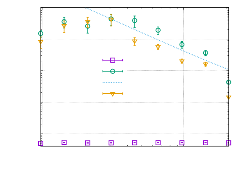
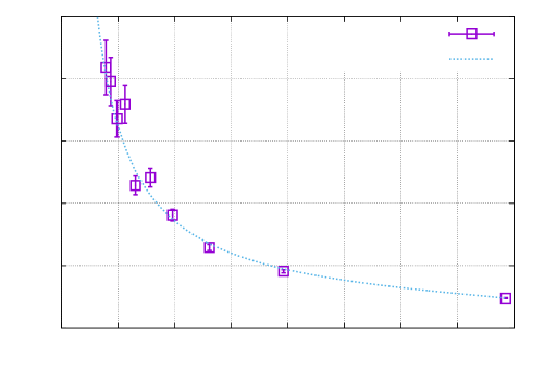
Figure 1 shows the integrated autocorrelation time $\tau_{\text{int}}$ in HMC simulations of Rubrene, a representative organic molecular semiconductor [5, 21, 23]. Electron numbers are very low in semiconductors $\left\langle n_{\text{el}}\right\rangle\approx 1\%$. Thus the electronic interaction term is very small, resulting in mere perturbations from the harmonic phonon action. Therefore, it does not come as a surprise that EFA consistently keeps autocorrelations low $\tau_{\text{int}}<1$ (completely uncorrelated data has $\tau_{\text{int}}=$0.5$$) throughout all simulations. Without FA we can expect from corollary 1 that $\tau_{\text{int}}$ will grow as the ratio of largest and smallest eigenvalues of $M_{\text{SSH}}$

$$\tau_{\text{int}} \propto 1+\left(\frac{2N_{t}}{\beta\omega_{0}}\right)^{2}\,.$$ (24)

Both scenarios of small $\omega_{0}$ (left) and large $N_{t}$ (right) are explored in figure 1 for two different observables (average electron $\left\langle n_{\text{el}}\right\rangle$ and phonon $\left\langle n_{\text{ph}}\right\rangle$ numbers). These scenarios are highly relevant in practice as the phonon frequency tends to be very small $\omega_{0}\ll 1/\beta$ in real materials and the limit $N_{t}\rightarrow\infty$ is required for the continuum limit. Even though the prefactors in $\tau_{\text{int}}$ clearly depend on the specific observable (as expected), the proportionality from corollary 1 is reproduced in all cases. The plateau in the right panel is an artefact of a limited number of trajectories.

Figure 2: Phonon number expectation value $\left\langle n_{\text{ph}}\right\rangle$ (left) and its autocorrelation function (right) in the 2+1D SSH model using HMC simulations [5] on a $10\times 10$ square lattice with $N_{t}=64$ imaginary time slices. The parameters $\beta=4$, $\omega_{0}=J_{\alpha}=g=1$, $\mu=0$ are particularly challenging, such that the system is clearly in the CDW-ordered phase but relatively close to the phase transition [17]. All simulations have similar compute time per measurement, but the acceptance is very low ($<10\%$) for long trajectories $T=\nicefrac{{\pi}}{{2}}$ because of numerical instabilities. Without FA the integrated autocorrelation time is $\tau_{\text{int}}=$1206(327)$$, with EFA it is $\tau_{\text{int}}(\nicefrac{{\pi}}{{20}})=$8.5(9)$$, $\tau_{\text{int}}(\nicefrac{{\pi}}{{6}})=$4.5(3)$$, $\tau_{\text{int}}(\nicefrac{{\pi}}{{2}})=$20.9(16)$$.

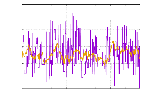
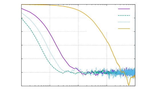
The regime investigated for figure 2 is crucially different from the previous one since these simulations are performed at half filling and the phonon-electron system is strongly interacting. A priori it is not clear how useful FA will be in this regime. However it stands to reason that the slowest phonon modes will still dominate autocorrelation, even though distorted by interactions. Therefore, we should expect EFA to significantly reduce autocorrelation, but not to remove it entirely. This is precisely what can be observed in figure 2. It shows the time series of the phonon expectation number and its autocorrelation function for the same physical parameters (in the CDW ordered phase) with and without EFA. Clearly, EFA reduces the autocorrelations by about two orders of magnitude.

The example in figure 2 is interesting as the optimal trajectory length with EFA appears to be significantly shorter than $T=\nicefrac{{\pi}}{{2}}$. The reason in this case is that the simulations involve matrix inverse and determinant calculations of badly conditioned matrices which leads to significant numerical errors. These errors accumulate more over longer trajectories so that the maximal possible acceptance (even with more MD steps) drops with growing trajectory length. As a consequence, it is beneficial to use shorter trajectories $T\approx\nicefrac{{\pi}}{{6}}$ in this case because of their higher acceptance and thus lower total autocorrelation.

3.2 The Ising model

Now, let us further investigate the importance of choosing the correct trajectory length. For this the Ising model in the HMC formulation of [25] is chosen because of its simplicity.

The Ising model describes classical spins $s_{i}=\pm 1$ with the coupling $J$ governed by the Hamiltonian

$$H_{\text{Ising}} =-J\sum_{\left\langle i,j\right\rangle}s_{i}s_{j}$$ (25)

$$=-\frac{1}{2}Js^{\mathsf{T}}Ks\,,$$ (26)

where $\left\langle i,j\right\rangle$ denotes nearest neighbours. After adding a large enough positive constant $C$ to the connectivity matrix $K$, to make $\tilde{K}\coloneqq K+C\mathbb{1}$ positive definite, an equivalent action

$$S_{\text{Ising}} =-\frac{1}{2J}\phi^{\mathsf{T}}\tilde{K}^{-1}\phi+\sum_{i}\log\cosh\phi_{i}$$ (27)

can be derived as in Ref. [25]. This action is formulated in terms of continuous fields $\phi$ and it includes a harmonic term, so that theorem 1 is applicable for EFA.

In two dimensions the classical Ising model features a phase transition [26]. At low couplings the spins are in a disordered phase and at high coupling they are ferromagnetically ordered. At the phase transition, most Monte Carlo simulation methods experience critical slowing down which means that the integrated autocorrelation time grows as $\tau_{\text{int}}\sim L^{z}$ with the lattice size $L$, where the dynamical exponent $z\simeq 2$ for the underlying HMC [25]. FA cannot overcome critical slowing down because this would require an increased tunnelling probability between different minima of the anharmonic potential while FA acts only on the harmonic components within a local minimum. However, FA can significantly reduce the coefficient in the $L^{z}$ divergence.

Figure 3: Integrated autocorrelation time $\tau_{\text{int}}$ of the absolute value of the magnetisation $|m|$ in the 2D Ising model using HMC simulations [25] on a $15\times 15$ lattice. Left: different coupling strengths ($J\approx$0.44$$ is the critical coupling [26]); Right: weak coupling $J=$0.2$$ and different trajectory lengths $T$. All simulations used EFA and have similar acceptance $\gtrsim 80\%$. The measurement frequency has been adjusted so that the HMC time between measurements is always the same. The dashed line shows the prediction for $\tau_{\text{int}}(T)=\tau_{\text{int}}(T=\nicefrac{{\pi}}{{2}})\cdot\left(1-\cos(T)^{\nicefrac{{\pi}}{{2T}}}\right)^{-1}$ from corollary 2.

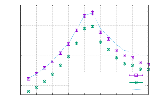
The peak of $\tau_{\text{int}}$ around the phase transition at $J\approx$0.44$$ is clearly visible in the left panel of figure 3. It is also clear that the coefficient of $\tau_{\text{int}}$ is larger for a suboptimal trajectory length over the entire parameter range. More specifically, corollary 2 predicts the coefficient exactly in the weakly coupled phase $J<$0.4$$ as expected for the region dominated by the harmonic potential. This is demonstrated even more vividly in the right panel of figure 3. The quantitative prediction fails in the strongly coupled anharmonic phase $J>$0.4$$, but the qualitative advantage of $T=\nicefrac{{\pi}}{{2}}$ as in theorem 1 over $T<\nicefrac{{\pi}}{{2}}$ is preserved.

In this example it appears that even longer trajectories $T>\nicefrac{{\pi}}{{2}}$ might reduce $\tau_{\text{int}}$ further. This is a consequence of the significant anharmonic part leading to $\tau_{\text{int}}\gg$0.5$$ even at $T=\nicefrac{{\pi}}{{2}}$. Since corollary 2 breaks down for longer trajectories, this phenomenon cannot be predicted analytically. Optimising longer trajectories coupling by coupling would therefore be up to numerical experiments. The advantage, however, is expected to be so small in most cases that it hardly warrants the additional work.

3.3 Lattice gauge theory

Our final example is motivated by lattice quantum chromodynamics (QCD), the theory describing quarks and gluons under the strong interaction. FA has been known in simulations of lattice QCD for decades. The original formulation in Refs. [27, 28] takes the structure of the underlying gauge group into account explicitly. It cannot be derived from theorem 1 and comes at the cost of numerical inversions or solves. In the following, an alternative idea how theorem 1 can be used in lattice QCD and gauge theories in general will be sketched. This approximate FA does not require numerical solves, but it does not mirror the exact group structure either. The approach is a generalisation of the FA used in Ref. [29] for quantum electrodynamics (QED) beyond the abelian U$(1)$ gauge group.

The goal of this section is to convey how broadly applicable theorem 1 is, even when it does not appear obvious. This proof-of-concept work does not aim to identify the most efficient simulation method for lattice gauge theories, it merely introduces another alternative to choose from in the future.

Any lattice gauge theory action [30] is of the form

$$S[U] =S_{G}[U]\,+\,\text{fermionic interactions}\,,$$ (28)

$$S_{G}[U] =\frac{\beta}{N_{c}}\sum_{n,\mu<\nu}\operatorname{Re}\operatorname{Tr}\left[1-U_{\mu\nu}(n)\right]\,,$$ (29)

where the fermionic part will not be considered further. Since the pure gauge part $S_{G}$ contains the harmonic potential, it will be accelerated in the following. The number of colours $N_{c}$ in the underlying SU$(N_{c})$ or U$(N_{c})$ group is left open deliberately. The plaquette

$$U_{\mu\nu}(n) =U_{\mu}(n)U_{\nu}(n+\mu)U_{\mu}(n+\nu)^{\dagger}U_{\nu}(n)^{\dagger}$$ (30)

is defined in the usual way as a function of the gauge links $U_{\mu}(n)$. Clearly, the action is not quadratic in the links, so theorem 1 is not applicable without further manipulations. Note that the gauge action is quadratic in the plaquette $S_{G}\sim\sum_{n,\mu<\nu}\operatorname{Tr}\left[(1-U_{\mu\nu}(n))^{\dagger}(1-U_{\mu\nu}(n))\right]$ and this property can be exploited for highly efficient sampling, for instance with the heat bath algorithm [31]. Unfortunately this ansatz does not generalise to HMC simulations because the EOM for plaquettes and their canonical momenta would inevitably violate unitarity (see section C.1 for more details).

In order to avoid such unitarity violations, one has to formulate the action in terms of the algebra rather than group elements, that is

$$U_{\mu}(n) =\mathrm{e}^{\operatorname{i}\frac{1}{2}x_{n,\mu}\cdot\lambda}\,,$$ (31)

where $\lambda$ is the vector of generators (Pauli spin matrices $\sigma$ for SU$(2)$, Gell-Mann matrices for SU$(3)$, etc.) and $x$ a vector field. As is derived in section C.2, the gauge action can be expanded around small values of $x$ and block-diagonalised via Fourier transformation

$$S_{G}(x) =\frac{1}{2}x^{\mathsf{T}}M_{G}x+\operatorname{\mathcal{O}}\left(x^{4}\right)\,,$$ (32)

$$=\frac{1}{2}\sum_{k,\mu,\nu}\left[y_{k,\mu}^{\dagger}\,M^{\mu\nu}_{G}(k)\,y_{k,\nu}^{\phantom{\dagger}}\right]+\operatorname{\mathcal{O}}\left(y^{4}\right)\,,$$ (33)

$$y_{k,\mu} =\frac{1}{\sqrt{N}}\sum_{n}\mathrm{e}^{-\operatorname{i}k\cdot n}x_{n,\mu}\,,$$ (34)

$$M^{\mu\nu}_{G}(k) =\frac{2\beta}{N_{c}}\left[\delta_{\mu\nu}\sum_{\rho}\sin^{2}\frac{k_{\rho}}{2}-\mathrm{e}^{\frac{\operatorname{i}}{2}\left(k_{\mu}-k_{\nu}\right)}\sin\frac{k_{\mu}}{2}\sin\frac{k_{\nu}}{2}\right]$$ (35)

with the lattice momenta $k$. The harmonic gauge matrix $M_{G}$ is defined by its action $M^{\mu\nu}_{G}(k)$ on the fields $y$ after Fourier transformation. On a hyper-cubic lattice in $d$ dimensions every site has $d$ associated links, so the remaining non-diagonal blocks are of dimensionality $d\times d$ and very fast to diagonalise numerically. At this point theorem 1 is directly applicable and momenta can be sampled accordingly. However, the EOM should be integrated numerically by taking the exact links $U_{\mu}(n)$ into account rather than their harmonic approximations, therefore no EFA is possible. An alternative approach to FA in gauge theories is sketched in section C.4.

The careful reader might have noticed that there is a minor problem in this formulation because the harmonic gauge matrix $M_{G}$ is not strictly positive definite. Zero momentum $k=0$ has eigenvalue zero. This makes sense because the gauge action is independent of the global gauge. Furthermore, a complete ‘band’ of zero eigenvalues corresponds to the eigenvectors of the form

$$y^{0}_{k,\mu} =\mathrm{e}^{\frac{\operatorname{i}}{2}k_{\mu}}\sin\frac{k_{\mu}}{2}.$$ (36)

This band captures the remaining local gauge degrees of freedom. Removing the dynamics of these zero modes, leads to a very natural gauge fixing which has been used for FA in this work (correctness is demonstrated in section C.3). An alternative approach could be to regulate the zeros by adding a small constant to $M_{G}$ the way classical FA typically proceeds.

Figure 4: Integrated autocorrelation time $\tau_{\text{int}}$ of the plaquette expectation value $\left\langle P(\beta)\right\rangle$ in pure gauge theory HMC simulations. Left: 2D, U$(1)$ weak coupling $\beta=$10$$ and different lattice sizes $L$; Right: 4D, $L=10$ lattice, SU$(3)$ and different coupling strengths $\beta$. All simulations required the same compute time per trajectory and volume. Measurements were performed every trajectory. Trajectory lengths without FA were chosen as follows. Left: $T=$0.6$$ tuned (by hand) to minimise $\tau_{\text{int}}$ on the $15\times 15$ lattice; Right: $T=1$ because it is the ‘canonical’ choice and $T=\nicefrac{{1}}{{\sqrt{\beta}}}$ because of its correct scaling from theorem 1.

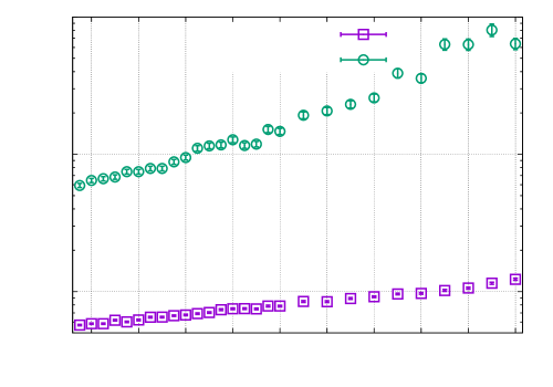
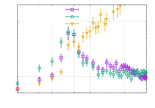
As derived in section C.2, the approximate FA is guaranteed to negate autocorrelation in the weak coupling (large $\beta$) regime. Both panels of figure 4 clearly show this behaviour. In particular, in the left panel 2D simulations of the U$(1)$ gauge group at weak coupling are presented for different lattice sizes. This is the regime required for realistic QED simulations and FA has proved very effective in this special case [29]. FA has an integrated autocorrelation time of the plaquette well below $\tau_{\text{int}}<2$ for all simulated sizes which is much lower than in all simulations without FA. In addition, $\tau_{\text{int}}$ with FA depends only very mildly on the system size compared to $\tau_{\text{int}}$ without FA (i.e. the slope on the log-scale is lower). This dependence is primarily caused by a decreasing acceptance as $L$ increases and it could be alleviated by either shortening the trajectory length (also increasing autocorrelation) or scaling the number of MD steps accordingly (increasing computation time per trajectory). Neither adjustment is necessary with FA. A further advantage of FA is that it does not require any tuning of the trajectory length while in the simulations without FA $T=$0.6$$ had to be tuned by hand in order to avoid even higher autocorrelation.

Just as in the Ising model simulations described in section 3.2, FA cannot remove autocorrelation intrinsically caused by anharmonic properties of the potential. For lattice gauge theories the so-called topological freezing can pose a severe problem [32]. Again, FA does not remove this effect, it only reduces the overall coefficient.

The right panel of figure 4 shows the integrated autocorrelation time in QCD-motivated simulations, i.e. in 4D with the SU$(3)$ gauge group. Simulations were performed on a relatively small lattice of length $L=10$ as a function of the coupling $\beta$. As expected, simulations with FA approach minimal autocorrelation for large $\beta>30$. $\tau_{\text{int}}$ with FA has a maximum at intermediate coupling $\beta\approx 5$. These results are compared to simulations without FA using fixed $T=1$ and adjusted $T=\nicefrac{{1}}{{\sqrt{\beta}}}$. The latter is already using insight from theorem 1, so technically it is harmonically accelerated, even though it does not rely on FA in the narrow sense.

The strong coupling limit $\beta\lesssim 1$ is very easy to simulate with and without FA, always yielding low autocorrelation. All simulations show an increase of $\tau_{\text{int}}$ towards intermediate coupling. The fixed trajectory length $T=1$ appears preferable below $\beta\lesssim 6$. However, this is an artefact of the excessively high number of molecular dynamics steps chosen here in order to observe the true decorrelation decoupled from acceptance influence. As long as the acceptance with $T=1$ is high enough, the longer trajectory allows better decorrelation. For weaker couplings $\beta>6$ (earlier in simulations with a realistic number of MD steps) this advantage vanishes because the acceptance goes to zero. In order to maintain a high acceptance at fixed $T=1$, one would need to scale the number of MD steps and thus computational effort with $\sqrt{\beta}$ which is clearly less efficient than to reduce the trajectory length by the same factor.

Qualitatively, $\tau_{\text{int}}$ behaves very similarly in simulations with FA and those without FA but with adjusted $T=\nicefrac{{1}}{{\sqrt{\beta}}}$. A priori this is not clear and it might well be that this similarity does not extend to observables other than the plaquette. The scaling with system size should favour FA, similarly to the simpler 2D example in the left panel of figure 4. For the given observable and lattice size there are still several small but significant differences. This approximate FA has been designed to work best in the weak coupling limit, accordingly it outperforms simulations without FA for large $\beta>50$. On the other hand, weak but not extreme coupling $10\lesssim\beta\lesssim 40$ favours simulations without FA. In this region, simulations with FA also took very many trajectories $\operatorname{\mathcal{O}}\left(1000\right)$ to thermalise. The origin of this bad performance is not yet understood. On a side note, decorrelation per accepted trajectory is usually slightly better with FA than without, but this is compensated by a slightly higher acceptance of simulations without FA and adjusted $T=\nicefrac{{1}}{{\sqrt{\beta}}}$.

Finally, theorem 1 only demands the proportionality $T\sqrt{\beta}=\text{const.}$, but the optimal coefficient cannot be fixed without further tuning (unless full FA is used). It is therefore very likely that $T=\nicefrac{{1}}{{\sqrt{\beta}}}$ is not even close to optimal. Moreover, the autocorrelation is strongly observable dependent, so that the best choice of $T$ might also depend on the observable of interest. For instance, in Ref. [33] the optimal trajectory length for slowly decorrelating observables at $\beta\approx 6$ is found empirically to be around $T\approx 2$, implying that $T=\nicefrac{{5}}{{\sqrt{\beta}}}$ might be a good choice.

Overall, the benchmark results are not conclusive and more testing, including comparisons to alternative simulation methods, will be needed. The optimal algorithm choice clearly depends the physical parameters. For abelian groups and for very weak couplings as in QED the approximate FA appears viable. The physically relevant coupling in QCD lies around $\beta\approx 6$, just in the region of maximal $\tau_{\text{int}}$. Thus, in this and similar regimes methods like the classical FA [27, 28] or no FA at all might be preferable.

4 Conclusion

In this work, the optimal parameters for hybrid Monte Carlo (HMC) simulations are explored. Theorem 1 presents a way to completely eliminate autocorrelations stemming from harmonic contributions of the action. The method relies on the analytic solution of the harmonic oscillator equations and is called exact Fourier acceleration (EFA), consistently with our previous (sub-optimal) formulation in Ref. [5]. It is summarised in algorithms 3, 1 and 2.

Since usually little to no analytic insight is available for anharmonic contributions to the action, EFA remains the best available method for most physical systems, far beyond the harmonically dominated case. One way to intuitively understand it, is that HMC with EFA reconciles the classical HMC ansatz with optimal sampling of normally distributed random variables. That is, for a purely harmonic action the HMC following theorem 1 coincides with uncorrelated sampling from a normal distribution, naturally generalising to more complicated actions without sacrificing performance.

The use of EFA often involves an FFT and always an adjustment of the HMC trajectory length. Both measures are computationally very cheap. Neglecting either of these adjustments can lead to an increase of the integrated autocorrelation time $\tau_{\text{int}}$ in simulations of physically relevant systems by many orders of magnitude (see figs. 1, 3). The functional dependences of $\tau_{\text{int}}$ on the condition number of the harmonic matrix and the trajectory length have been quantified in corollaries 1 and 2, respectively. Both theoretical predictions have been found in excellent agreement with data obtained in numerical simulations of the SSH and the Ising models.

In section 3.3 an approximate form of Fourier acceleration (FA) has been applied to lattice gauge theory. It worked very well in the abelian case, relevant for quantum electrodynamics (QED), but the results for non-abelian gauge groups, required e.g. for quantum chromodynamics (QCD), remain inconclusive. Apart from the very weakly coupled regime where the FA becomes exact, it is not clear whether FA can outperform more conventional methods. The answer appears parameter-dependent and will require further case-by-case tuning or, ideally, an improved version of the FA. Nevertheless, the insight from theorem 1 still proved useful for the simulation of lattice gauge theories, as it provides us with the optimal scaling of the trajectory length with the coupling $T\propto\nicefrac{{1}}{{\sqrt{\beta}}}$.

For all its merits, EFA does not help the HMC to avoid critical slowing down because it only optimises sampling within a local minimum of the action. EFA does not introduce any mechanism to overcome potential barriers (see fig. 3, left). In this sense it is neither advantageous nor disadvantageous compared to classical HMC. For systems with de-facto ergodicity problems like topological freezing additional methods have to be combined with EFA in order to guarantee efficient sampling. Finding these methods is, of course, a very challenging task and the search will go on.

Code and Data

The simulations of the Ising model in section 3.2 have been performed with a modified version of the code [34] published with Ref. [25]. The code for the SSH model simulations in section 3.1 has been published recently [35], accompanying an updated version of Ref. [5]. The lattice gauge theory code [36] used in section 3.3 has been written from scratch for this work. The analysis used the light-weight tool comp-avg [37]. All these codes are implemented in C and have been published under open access. Most of the simulations in this work can be reproduced very quickly, nonetheless the resulting data will gladly be provided upon request.

Appendix A Proofs of corollaries 1 and 2

Proof: no Fourier acceleration, corollary 1.

In order to maintain a constant acceptance rate and computational cost per trajectory, the trajectory length has to be chosen so that $\omega_{\mathrm{max}}T=\text{const.}$ because (unless in a null set of cases some periodic behaviour is achieved) the fastest mode is responsible for the biggest changes after a fixed (short) time and therefore dominates the acceptance. We set

$$T =\frac{\alpha}{\omega_{\mathrm{max}}}$$ (37)

with some positive constant $\alpha$. Autocorrelation, on the other hand, is primarily caused by the slowest mode that requires most HMC steps to change significantly. The autocorrelation of the configuration $x$ is thus dominated by

$$\frac{\left\langle x_{i_{\text{min}}}\left(\frac{\alpha}{\omega_{\mathrm{max}}}\right)\,x_{i_{\text{min}}}^{0}\right\rangle}{\left\langle\left(x_{i_{\text{min}}}^{0}\right)^{2}\right\rangle} =\frac{\left\langle x_{i_{\text{min}}}^{0}\,x_{i_{\text{min}}}^{0}\right\rangle}{\left\langle\left(x_{i_{\text{min}}}^{0}\right)^{2}\right\rangle}\cos\left(\alpha\frac{\omega_{\text{min}}}{\omega_{\mathrm{max}}}\right)+\frac{\left\langle p_{i_{\text{min}}}^{0}\,x_{i_{\text{min}}}^{0}\right\rangle}{\left\langle\left(x_{i_{\text{min}}}^{0}\right)^{2}\right\rangle}\frac{\sin\left(\alpha\frac{\omega_{\text{min}}}{\omega_{\mathrm{max}}}\right)}{\omega_{\text{min}}}$$ (38)

$$=\cos\left(\alpha\frac{\omega_{\text{min}}}{\omega_{\mathrm{max}}}\right)\,,$$ (39)

where $i_{\text{min}}$ is the index corresponding to the slowest mode $\omega_{\mathrm{min}}$. For $x(T)$ the explicit formula (10) has been used. The sin-term can be dropped because $x^{0}$ and $p^{0}$ are uncorrelated, i.e. $\left\langle x_{i}^{0}p_{i}^{0}\right\rangle=\left\langle x_{i}^{0}\right\rangle\left\langle p_{i}^{0}\right\rangle$, and $\left\langle p^{0}\right\rangle=0$.

The correlation after $n$ trajectories is given by the power $\cos\left(\alpha\frac{\omega_{\text{min}}}{\omega_{\mathrm{max}}}\right)^{n}$ and the integrated autocorrelation time is directly proportional to the geometric series over the correlation function

$$\tau_{\mathrm{int}} \propto\sum_{n=0}^{\infty}\cos\left(\alpha\frac{\omega_{\text{min}}}{\omega_{\mathrm{max}}}\right)^{n}$$ (40)

$$=\left(1-\cos\left(\alpha\frac{\omega_{\mathrm{min}}}{\omega_{\mathrm{max}}}\right)\right)^{-1}$$ (41)

$$=2\left(\alpha^{-1}\frac{\omega_{\mathrm{max}}}{\omega_{\mathrm{min}}}\right)^{2}+\frac{1}{6}+\operatorname{\mathcal{O}}\left(\left(\frac{\omega_{\mathrm{min}}}{\omega_{\mathrm{max}}}\right)^{2}\right)\,.$$ (42)

∎

Proof: too short trajectory, corollary 2.

The proof proceeds very similarly to that of corollary 1 with two differences. First of all the FA rescales all frequencies $\omega_{i}$ by their inverse, so the correlation (39) after a single trajectory simplifies to

$$\frac{\left\langle x_{i}\left(T\right)\,x_{i}^{0}\right\rangle}{\left\langle\left(x_{i}^{0}\right)^{2}\right\rangle} =\cos(T)$$ (43)

for all $i$. Secondly, a shorter trajectory comes with reduced computational cost, so a fair comparison is only ensured when proportionally rarer measurements are conducted. The fictitious HMC time between measurements (equivalent to the computational cost) is kept fixed by measuring only every $\frac{\pi}{2T}$-th trajectory with respect to the measurement frequency of $T=\frac{\pi}{2}$. After $\frac{\pi}{2T}$ trajectories the correlation is given by $\cos(T)^{\nicefrac{{\pi}}{{2T}}}$ and the geometric series therefore amounts to

$$\tau_{\mathrm{int}}(T) =\tau_{\mathrm{int}}(T=\nicefrac{{\pi}}{{2}})\sum_{n=0}^{\infty}\cos(T)^{n\nicefrac{{\pi}}{{2T}}}$$ (44)

$$=\frac{\tau_{\mathrm{int}}(T=\nicefrac{{\pi}}{{2}})}{1-\cos(T)^{\nicefrac{{\pi}}{{2T}}}}\,.$$ (45)

∎

Appendix B The Hubbard model

The Hubbard model [38] is mentioned here as an example of pure “harmonic” acceleration without the need to perform a Fourier transformation since the matrix $M\propto\mathbb{1}$ in the action (6) is already diagonal in real space.

The Hamiltonian defining the Hubbard model reads

$$H_{\text{Hub}} =-\kappa\sum_{\left\langle x,y\right\rangle,\sigma}\left(c^{\dagger}_{x,\sigma}c^{\phantom{\dagger}}_{y,\sigma}+c^{\dagger}_{y,\sigma}c^{\phantom{\dagger}}_{x,\sigma}\right)+U\sum_{x}n_{x\uparrow}n_{x\downarrow}\,,$$ (46)

where $\kappa$ denotes the hopping amplitude between nearest neighbours $\left\langle x,y\right\rangle$ and $U$ is the (repulsive) on-site interaction strength. The creation (annihilation) operators $c^{\dagger}_{x,\sigma}$ ($c^{\phantom{\dagger}}_{x,\sigma}$) and corresponding number operators $n_{x,\sigma}\equiv c^{\dagger}_{x,\sigma}c^{\phantom{\dagger}}_{x,\sigma}$ represent fermions (e.g. electrons) of spin $\sigma$ at site $x$.

Following the formalism of Refs. [39, 40, 41] and setting $\tilde{U}\coloneqq\frac{\beta U}{N_{t}}$, the grand-canonical action

$$S_{\text{Hub}}(\phi) =\frac{1}{2\tilde{U}}\phi^{2}+\text{interactions}$$ (47)

$$\xRightarrow{\text{th.\leavevmode\nobreak\ \ref{th:opt_traj_and_kin}}}\mathcal{H}_{\text{Hub}} =\frac{\tilde{U}}{2}p^{2}+S_{\text{Hub}}(\phi)$$ (48)

at inverse temperature $\beta$ can be derived. The number of Euclidean time slices $N_{t}$ has to be large $N_{t}\gg\beta U$ in order to approach the continuum limit, so typically the ‘mass’ of the canonical momenta $p$ associated with the Hubbard–Stratonovich fields $\phi$ should be chosen larger than unity as well.

As mentioned before, the harmonic matrix $M_{\text{Hub}}=\frac{1}{2\tilde{U}}\mathbb{1}$ is proportional to the identity. Therefore, all masses should be chosen equal according to theorem 1. In fact, for simplicity’s sake, the momenta $p$ can be sampled from a standard normal distribution $\mathcal{H}_{\text{Hub}}=\frac{1}{2}p^{2}+S_{\text{Hub}}(\phi)$ with the only degree of freedom absorbed into the trajectory length $T=\frac{\pi}{2}\sqrt{\tilde{U}}$.

Appendix C Accelerating lattice gauge theory simulations

C.1 Why heat bath cannot be generalised

The heat bath algorithm [31, 30] is an efficient way to sample new link variables locally in pure gauge theory. It effectively removes the potential rejection in standard Metropolis Hastings sampling. The heat bath uses the property that the gauge action $S_{G}$ is quadratic in the plaquette $U_{\mu\nu}(n)$

$$S_{G}[U] =\frac{\beta}{2N_{c}}\sum_{n,\mu<\nu}\operatorname{Tr}\left[(1-U_{\mu\nu}(n))^{\dagger}(1-U_{\mu\nu}(n))\right]\,.$$ (49)

This allows to sample the plaquette very easily. So choosing a link, sampling all adjacent plaquettes while keeping the corresponding staples constant, and multiplying the plaquette by the inverse sum of staples, leads to an optimal update of the link.

Unfortunately, this updating scheme cannot be generalised to HMC type sampling because it operates in the group rather than the algebra. So, if we sample momenta corresponding to the group elements, the EOM will bring us out of the group. We could rescale the result to project it back into the group, but this changes the action, so most likely the update will be rejected. Heat bath only works because it does not require the link and corresponding plaquette to remain within the group over a continuous trajectory, only at discrete special time steps.

On a more abstract level, the problem is that we do not sample in flat space but on a manifold with non-trivial Haar measure which is not included in the action.

C.2 Derivation of the approximative FA

We write equation (31) in the compact way

$$U_{\mu}(n) =\mathrm{e}^{\operatorname{i}\Lambda_{\mu}(n)}\,,$$ (50)

$$\Lambda_{\mu}(n) =\frac{1}{2}x_{n,\mu}\cdot\lambda\,,$$ (51)

so that the plaquette can be expanded in small values of $\Lambda$

$$U_{\mu\nu}(n) =U_{\mu}(n)U_{\nu}(n+\mu)U_{\mu}(n+\nu)^{\dagger}U_{\nu}(n)^{\dagger}$$ (52)

$$=\mathrm{e}^{\operatorname{i}\Lambda_{\mu}(n)}\mathrm{e}^{\operatorname{i}\Lambda_{\nu}(n+\mu)}\mathrm{e}^{-\operatorname{i}\Lambda_{\mu}(n+\nu)}\mathrm{e}^{-\operatorname{i}\Lambda_{\nu}(n)}$$ (53)

$$\begin{split}&=\left(1+\operatorname{i}\Lambda_{\mu}(n)-\frac{1}{2}\Lambda_{\mu}(n)^{2}\right)\left(1+\operatorname{i}\Lambda_{\nu}(n+\mu)-\frac{1}{2}\Lambda_{\nu}(n+\mu)^{2}\right)\\ &\quad\times\left(1-\operatorname{i}\Lambda_{\mu}(n+\nu)-\frac{1}{2}\Lambda_{\mu}(n+\nu)^{2}\right)\left(1-\operatorname{i}\Lambda_{\nu}(n)-\frac{1}{2}\Lambda_{\nu}(n)^{2}\right)\\ &\quad+\operatorname{\mathcal{O}}\left(\Lambda^{3}\right)\,.\end{split}$$ (54)

Under the (real part of the) trace required for the action only the even orders of $\Lambda$ survive

$$\begin{split}\operatorname{Re}\operatorname{Tr}\left[1-U_{\mu\nu}(n)\right]&=\operatorname{Re}\operatorname{Tr}\left[\vphantom{\frac{1}{2}}\Lambda_{\mu}(n)\Lambda_{\nu}(n+\mu)-\Lambda_{\mu}(n)\Lambda_{\mu}(n+\nu)-\Lambda_{\mu}(n)\Lambda_{\nu}(n)\right.\\ &\qquad-\Lambda_{\nu}(n+\mu)\Lambda_{\mu}(n+\nu)-\Lambda_{\nu}(n+\mu)\Lambda_{\nu}(n)+\Lambda_{\mu}(n+\nu)\Lambda_{\nu}(n)\\ &\qquad\left.+\frac{1}{2}\left(\Lambda_{\mu}(n)^{2}+\Lambda_{\nu}(n+\mu)^{2}+\Lambda_{\mu}(n+\nu)^{2}+\Lambda_{\nu}(n)^{2}\right)\right]+\operatorname{\mathcal{O}}\left(\Lambda^{4}\right)\end{split}$$ (55)

$$\begin{split}&=\frac{1}{2}\left[\vphantom{\frac{1}{2}}x_{n,\mu}\cdot x_{n+\mu,\nu}-x_{n,\mu}\cdot x_{n+\nu,\mu}-x_{n,\mu}\cdot x_{n,\nu}\right.\\ &\qquad-x_{n+\mu,\nu}\cdot x_{n+\nu,\mu}-x_{n+\mu,\nu}\cdot x_{n,\nu}+x_{n+\nu,\mu}\cdot x_{n,\nu}\\ &\qquad\left.+\frac{1}{2}\left(x_{n,\mu}^{2}+x_{n+\mu,\nu}^{2}+x_{n+\nu,\mu}^{2}+x_{n,\nu}^{2}\right)\right]+\operatorname{\mathcal{O}}\left(x^{4}\right)\end{split}$$ (56)

because all generators of SU$(N_{c})$ are traceless (in case of U$(N_{c})$ only the identity has non-zero trace and its odd power contributions are purely imaginary). In the step from $\Lambda$ to $x$ the generator orthogonality under the trace

$$\frac{1}{4}\operatorname{Tr}\left[\lambda_{i}\lambda_{k}\right] =\frac{1}{2}\delta_{ik}$$ (57)

was used.

Reintroducing the sum in the pure gauge action, allows to shift a number of indices, so that a Fourier transformation can be used to diagonalise the expression in real space

$$S_{G}(x) =\frac{\beta}{N_{c}}\sum_{n,\mu<\nu}\operatorname{Re}\operatorname{Tr}\left[1-U_{\mu\nu}(n)\right]$$ (58)

$$=\frac{\beta}{2N_{c}}\sum_{n,\mu,\nu}\operatorname{Re}\operatorname{Tr}\left[1-U_{\mu\nu}(n)\right]$$ (59)

$$\begin{split}&=\frac{\beta}{4N_{c}}\sum_{n,\mu,\nu}\left[x_{n,\mu}\cdot x_{n+\mu,\nu}-x_{n,\mu}\cdot x_{n+\nu,\mu}-x_{n,\mu}\cdot x_{n,\nu}\right.\\ &\qquad-x_{n,\mu}\cdot x_{n+\mu-\nu,\nu}-x_{n,\mu}\cdot x_{n-\nu,\mu}+x_{n,\mu}\cdot x_{n-\nu,\nu}\\ &\qquad\left.+2x_{n,\mu}^{2}\right]+\operatorname{\mathcal{O}}\left(x^{4}\right)\end{split}$$ (60)

$$\begin{split}&=\frac{\beta}{4N_{c}}\sum_{k,\mu,\nu}\left[\mathrm{e}^{\operatorname{i}k_{\mu}}y_{k,\mu}^{\dagger}\cdot y_{k,\nu}^{\phantom{\dagger}}-\mathrm{e}^{\operatorname{i}k_{\nu}}y_{k,\mu}^{\dagger}\cdot y_{k,\mu}^{\phantom{\dagger}}-y_{k,\mu}^{\dagger}\cdot y_{k,\nu}^{\phantom{\dagger}}\right.\\ &\qquad-\mathrm{e}^{\operatorname{i}(k_{\mu}-k_{\nu})}y_{k,\mu}^{\dagger}\cdot y_{k,\nu}^{\phantom{\dagger}}-\mathrm{e}^{-\operatorname{i}k_{\nu}}y_{k,\mu}^{\dagger}\cdot y_{k,\mu}^{\phantom{\dagger}}+\mathrm{e}^{-\operatorname{i}k_{\mu}}y_{k,\mu}^{\dagger}\cdot y_{k,\nu}^{\phantom{\dagger}}\\ &\qquad\left.+2\left|y_{k,\mu}\right|^{2}\right]+\operatorname{\mathcal{O}}\left(y^{4}\right)\,,\end{split}$$ (61)

$$y_{k,\mu} =\frac{1}{\sqrt{N}}\sum_{n}\mathrm{e}^{-\operatorname{i}k\cdot n}x_{n,\mu}\,.$$ (62)

This result can be expressed more compactly with the help of some trigonometric identities

$$S_{G}(y) =\frac{\beta}{N_{c}}\sum_{k,\mu,\nu}\left[\left|y_{k,\mu}\right|^{2}\sin\frac{k_{\nu}}{2}-y_{k,\mu}^{\dagger}\cdot y_{k,\nu}^{\phantom{\dagger}}\,\mathrm{e}^{\operatorname{i}(k_{\mu}-k_{\nu})}\sin\frac{k_{\mu}}{2}\sin\frac{k_{\nu}}{2}\right]\,,$$ (63)

obtaining the elegant form used in equation (35). Note that, induced by the dimensionality of $x$, each component of $y$ is a vector $y_{k,\mu}\in\mathbb{C}^{N_{\mathfrak{g}}}$ where $N_{\mathfrak{g}}$ is the number of generators $\lambda$, or equivalently the dimension of the corresponding Lie algebra. $M_{G}$ acts trivially within this space.

It is not straight forward to diagonalise the harmonic gauge matrix $M_{G}(k)$ analytically. However, the two distinct eigenvalues can be determined exactly and a (non-orthogonal) basis for each of the eigen-subspaces can be provided as follows. Let

$$y^{0}_{k} =\sum_{\mu}\mathrm{e}^{\frac{\operatorname{i}}{2}k_{\mu}}\sin\frac{k_{\mu}}{2}\,\hat{e}_{\mu}\,,$$ (64)

$$y^{i}_{k} =\mathrm{e}^{\frac{\operatorname{i}}{2}k_{\alpha}}\sin\frac{k_{i}}{2}\,\hat{e}_{\alpha}-\mathrm{e}^{\frac{\operatorname{i}}{2}k_{i}}\sin\frac{k_{\alpha}}{2}\,\hat{e}_{i}$$ (65)

with $\hat{e}_{\mu}$ the standard normal basis vectors. Here, in $d$ spatial dimensions, $i=1,\dots,d-1$ and $\alpha\in\{0,\dots,d-1\}$ is an arbitrary but fixed index so that $\sin\frac{k_{\alpha}}{2}\neq 0$. Then it is easy to check that the $y^{0}_{k}$, $y^{i}_{k}$ are eigenvectors of $M_{G}(k)$ with eigenvalues given by

$$M_{G}(k)\,y^{0}_{k} =0\,,$$ (66)

$$M_{G}(k)\,y^{i}_{k} =\left(\sum_{\mu}\sin^{2}\frac{k_{\mu}}{2}\right)y^{i}_{k}\,.$$ (67)

In practice, an efficient way to construct an orthonormal set of eigenvectors is to simply orthonormalise the raw eigenvectors $y^{\mu}_{k}$ using e.g. the modified Gram-Schmidt process.

This approximation works best in the weak coupling regime. Asymptotically as $\beta\rightarrow\infty$, it becomes exact and the FA based on this method is guaranteed to completely decorrelate the configurations after a single trajectory. For abelian groups the expansion is identical about every group element, not just the identity. Therefore, FA is guaranteed to work very well with abelian groups if the plaquette is close enough to the identity, even if the individual links are not. For non-abelian groups no such guarantee can be given as long as not all the links are close to the identity. In practice, however, this does not appear to be a major problem.

C.3 Numerical verification of the approximate FA

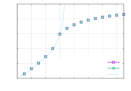
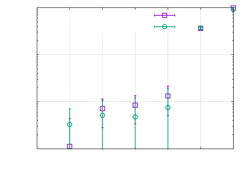
We benchmark the results of our numerical HMC simulations with and without FA against the strong coupling expansion in figure 5. Refs. [42, 43] provide explicit formulae for the free energy $F$ up to 16th order. The free energy can be translated to the plaquette expectation value as

$$\left\langle P(\beta)\right\rangle \equiv\left\langle\frac{1}{L^{d}}\sum_{n}\frac{2}{d(d-1)}\sum_{\mu<\nu}\frac{1}{N_{c}}\operatorname{Re}\operatorname{Tr}\left[U_{\mu\nu}(n)\right]\right\rangle$$ (68)

$$=\frac{2}{d(d-1)\,N_{c}!}\,\frac{\mathrm{d}}{\mathrm{d}\beta}F\left(\frac{\beta}{N_{c}!}\right)\,.$$ (69)

As expected, we find excellent agreement between all the methods for the strong coupling regime $\beta\lesssim 4$ and the two numerical methods agree within errors for the entire tested parameter range.

Figure 5: Plaquette results in SU$(3)$ pure gauge theory on a $10^{4}$ lattice from HMC simulations checked against the strong coupling expansion [42, 43] using eq. (69). The 16th order expansion was converted to Padé approximation form in order to maximise the range of validity. Left: plaquette expectation value $\left\langle P(\beta)\right\rangle$; Right: absolute value of the deviation of $\left\langle P(\beta)\right\rangle$ from eq. (69).

C.4 Alternative approach sampling the plaquette

From section C.1 we learn that we have to sample in the algebra, as is done in classical lattice QCD HMC simulations for exactly this reason. One alternative option to sampling the links as in section C.2 is to still sample the plaquette like heat bath does. This means that we would also have to choose a subset of links to update at a time, but this subset can be extensive in the volume, so an update would still be global. Expand the plaquette $U_{\mu\nu}(n)=\exp\left(\operatorname{i}X_{n,\mu\nu}\right)$ around unity to obtain $S_{G}\sim\beta X^{2}$. Now sample momenta according to this harmonic part and then evolve the EOM using the force from the full action.

If $\beta$ is large, then deviations from unity will be strongly suppressed, so the harmonic part can be solved exactly (i.e. with EFA) and the deviation of the gauge action from the harmonic approximation can be treated as part of the perturbation. If $\beta$ is not very large, then the approximation is not very good either and it makes more sense to use the full action for updates directly and only make discrete time steps. In any case, sampling momenta according to this distribution should be close to optimal for the decorrelation.

The advantage of this ansatz over the link sampling in section C.2 is that the $U_{\mu}(n)$ are not required to be close to the identity link by link. It suffices that the plaquette is close to the identity. In addition, no Fourier transformation is involved. On the other hand $\operatorname{\mathcal{O}}\left(d^{2}\right)$ updates are required for a full update of all links, as opposed to a single global update in section C.2. This overhead might be especially crucial when expensive fermionic updates are involved.

Overall, this method and the link sampling both appear viable. Potentially, the plaquette sampling is advantageous at moderately weak coupling where the plaquettes are close to unity but the links are not.

References

- [1] S. Duane, A. D. Kennedy, B. J. Pendleton and D. Roweth “Hybrid Monte Carlo” In Phys. Lett. B 195, 1987, pp. 216 –222 URL: https://doi.org/10.1016/0370-2693(87)91197-X
- [2] G. G. Batrouni et al. “Langevin simulations of lattice field theories” In Phys. Rev. D 32 American Physical Society, 1985, pp. 2736–2747 DOI: 10.1103/PhysRevD.32.2736
- [3] C. Urbach, K. Jansen, A. Shindler and U. Wenger “HMC algorithm with multiple time scale integration and mass preconditioning” In Computer Physics Communications 174.2, 2006, pp. 87–98 DOI: https://doi.org/10.1016/j.cpc.2005.08.006
- [4] B. Cohen-Stead et al. “Fast and scalable quantum Monte Carlo simulations of electron-phonon models” In Phys. Rev. E. 105, 2022, pp. 065302 URL: http://dx.doi.org/10.1103/PhysRevE.105.065302
- [5] Johann Ostmeyer, Tahereh Nematiaram, Alessandro Troisi and Pavel Buividovich “First-principle quantum Monte-Carlo study of charge carrier mobility in organic molecular semiconductors”, 2023 DOI: 10.48550/arXiv.2312.14914
- [6] I.P. Omelyan, I.M. Mryglod and R. Folk “Symplectic analytically integrable decomposition algorithms: classification, derivation, and application to molecular dynamics, quantum and celestial mechanics simulations” In Computer Physics Communications 151.3, 2003, pp. 272–314 DOI: https://doi.org/10.1016/S0010-4655(02)00754-3
- [7] R. Blankenbecler, D. J. Scalapino and R. L. Sugar “Monte Carlo calculations of coupled boson-fermion systems. I” In Phys. Rev. D 24 American Physical Society, 1981, pp. 2278–2286 DOI: 10.1103/PhysRevD.24.2278
- [8] Esteban G. Tabak and Eric Vanden-Eijnden “Density estimation by dual ascent of the log-likelihood” In Communications in Mathematical Sciences 8.1 International Press of Boston, Inc., 2010, pp. 217–233 DOI: 10.4310/CMS.2010.v8.n1.a11
- [9] Ivan Kobyzev, Simon J.D. Prince and Marcus A. Brubaker “Normalizing Flows: An Introduction and Review of Current Methods” In IEEE Transactions on Pattern Analysis and Machine Intelligence 43.11 Institute of ElectricalElectronics Engineers (IEEE), 2021, pp. 3964–3979 DOI: 10.1109/tpami.2020.2992934
- [10] Ulli Wolff “Monte Carlo errors with less errors” In Computer Physics Communications 156.2, 2004, pp. 143–153 DOI: https://doi.org/10.1016/S0010-4655(03)00467-3
- [11] Loup Verlet “Computer "Experiments" on Classical Fluids. I. Thermodynamical Properties of Lennard-Jones Molecules” In Phys. Rev. 159 American Physical Society, 1967, pp. 98–103 DOI: 10.1103/PhysRev.159.98
- [12] Johann Ostmeyer “Optimised Trotter decompositions for classical and quantum computing” In J. Phys. A 56.28 IOP Publishing, 2023, pp. 285303 DOI: 10.1088/1751-8121/acde7a
- [13] A.D. Kennedy and Brian Pendleton “Acceptances and autocorrelations in hybrid Monte Carlo” In Nuclear Physics B - Proceedings Supplements 20, 1991, pp. 118–121 DOI: https://doi.org/10.1016/0920-5632(91)90893-J
- [14] Benjamin Cohen-Stead et al. “SmoQyDQMC.jl: A flexible implementation of determinant quantum Monte Carlo for Hubbard and electron-phonon interactions”, 2024 arXiv:2311.09395 [cond-mat.str-el]
- [15] Matthew D. Homan and Andrew Gelman “The No-U-turn sampler: adaptively setting path lengths in Hamiltonian Monte Carlo” In J. Mach. Learn. Res. 15.47, 2014, pp. 1593–1623 arXiv: http://jmlr.org/papers/v15/hoffman14a.html
- [16] W. P. Su, J. R. Schrieffer and A. J. Heeger “Solitons in Polyacetylene” In Phys. Rev. Lett. 42 American Physical Society, 1979, pp. 1698–1701 DOI: 10.1103/PhysRevLett.42.1698
- [17] Bo Xing et al. “Quantum Monte Carlo Simulations of the 2D Su-Schrieffer-Heeger Model” In Phys. Rev. Lett. 126 American Physical Society, 2021, pp. 017601 DOI: 10.1103/PhysRevLett.126.017601
- [18] A. Götz, S. Beyl, M. Hohenadler and F. F. Assaad “Valence-bond solid to antiferromagnet transition in the two-dimensional Su-Schrieffer-Heeger model by Langevin dynamics” In Phys. Rev. B 105, 2022, pp. 085151 URL: http://dx.doi.org/10.1103/PhysRevB.105.085151
- [19] X. Cai, Z.-X. Li and H. Yao “High-temperature superconductivity induced by the Su-Schrieffer-Heeger electron-phonon coupling”, 2023 eprint: 2308.06222
- [20] G. G. Batrouni and Richard T. Scalettar “Langevin simulations of a long-range electron-phonon model” In Phys. Rev. B 99 American Physical Society, 2019, pp. 035114 DOI: 10.1103/PhysRevB.99.035114
- [21] S. Fratini et al. “A map of high-mobility molecular semiconductors” In Nature Materials 16, 2017, pp. 998 – 1002 URL: http://dx.doi.org/10.1038/nmat4970
- [22] S. Fratini et al. “Charge transport in high-mobility conjugated polymers and molecular semiconductors” In Nat. Mater. 19, 2020, pp. 491 –502 URL: http://dx.doi.org/10.1038/s41563-020-0647-2
- [23] D. Vong et al. “Quantitative Hole Mobility Simulation and Validation in Substituted Acenes” In J. Phys. Chem. Lett. 13, 2022, pp. 5530 –5537 URL: http://dx.doi.org/10.1021/acs.jpclett.2c00898
- [24] Maksim Ulybyshev, Nils Kintscher, Karsten Kahl and Pavel Buividovich “Schur complement solver for Quantum Monte-Carlo simulations of strongly interacting fermions” In Computer Physics Communications 236 Elsevier BV, 2019, pp. 118–127 DOI: 10.1016/j.cpc.2018.10.023
- [25] Johann Ostmeyer et al. “The Ising Model with Hybrid Monte Carlo” In Comput. Phys. Commun. 265, 2021, pp. 107978 DOI: 10.1016/j.cpc.2021.107978
- [26] Lars Onsager “Crystal Statistics. I. A Two-Dimensional Model with an Order-Disorder Transition” In Phys. Rev. 65 American Physical Society, 1944, pp. 117–149 DOI: 10.1103/PhysRev.65.117
- [27] Simon Duane, Richard Kenway, Brian J. Pendleton and Duncan Roweth “Acceleration of gauge field dynamics” In Physics Letters B 176.1, 1986, pp. 143–148 DOI: https://doi.org/10.1016/0370-2693(86)90940-8
- [28] Simon Duane and Brian J. Pendleton “Gauge invariant Fourier acceleration” In Physics Letters B 206.1, 1988, pp. 101–106 DOI: https://doi.org/10.1016/0370-2693(88)91270-1
- [29] Sz. Borsanyi et al. “Ab initio calculation of the neutron-proton mass difference” In Science 347.6229, 2015, pp. 1452–1455 DOI: 10.1126/science.1257050
- [30] Christof Gattringer and Christian B. Lang “Quantum chromodynamics on the lattice” ISBN: 978-3-642-01849-7 Berlin: Springer, 2010 DOI: 10.1007/978-3-642-01850-3
- [31] Michael Creutz “Monte Carlo study of quantized SU(2) gauge theory” In Phys. Rev. D 21 American Physical Society, 1980, pp. 2308–2315 DOI: 10.1103/PhysRevD.21.2308
- [32] Stefan Schaefer, Rainer Sommer and Francesco Virotta “Critical slowing down and error analysis in lattice QCD simulations” In Nucl. Phys. B 845, 2011, pp. 93–119 DOI: 10.1016/j.nuclphysb.2010.11.020
- [33] Harvey Meyer et al. “Exploring the HMC trajectory-length dependence of autocorrelation times in lattice QCD” In Computer Physics Communications 176.2, 2007, pp. 91–97 DOI: https://doi.org/10.1016/j.cpc.2006.08.002
- [34] Johann Ostmeyer “ising_hmc” updeated version with FA on branch ‘fourier_acc’ In GitHub repository GitHub, https://github.com/HISKP-LQCD/ising_hmc, 2024
- [35] Johann Ostmeyer and Pavel Buividovich “HMC simulations of electron-phonon systems” https://github.com/j-ostmeyer/electron-phonon-hmc Zenodo, 2024 DOI: 10.5281/zenodo.10973014
- [36] Johann Ostmeyer “Lattice Gauge Theory with HMC and Fourier Acceleration” https://github.com/j-ostmeyer/lattice_gauge_fa Zenodo, 2024 DOI: 10.5281/zenodo.10810716
- [37] Johann Ostmeyer “comp-avg: Compare Averages of time series and more” https://github.com/j-ostmeyer/comp-avg Zenodo, 2024 DOI: 10.5281/zenodo.10794620
- [38] J. Hubbard “Electron Correlations in Narrow Energy Bands” In Proceedings of the Royal Society of London. Series A, Mathematical and Physical Sciences 276.1365 The Royal Society, 1963, pp. 238–257 DOI: 10.1098/rspa.1963.0204
- [39] Thomas Luu and Timo A. Lähde “Quantum Monte Carlo calculations for carbon nanotubes” In Phys. Rev. B 93 American Physical Society, 2016, pp. 155106 DOI: 10.1103/PhysRevB.93.155106
- [40] Stefan Krieg et al. “Accelerating Hybrid Monte Carlo simulations of the Hubbard model on the hexagonal lattice” In Comput. Phys. Commun. 236, 2019, pp. 15 –25 DOI: 10.1016/j.cpc.2018.10.008
- [41] Johann Ostmeyer et al. “Semimetal–Mott insulator quantum phase transition of the Hubbard model on the honeycomb lattice” In Phys. Rev. B 102 American Physical Society, 2020, pp. 245105 DOI: 10.1103/PhysRevB.102.245105
- [42] R. Balian, J. M. Drouffe and C. Itzykson “Gauge fields on a lattice. III. Strong-coupling expansions and transition points” In Phys. Rev. D 11 American Physical Society, 1975, pp. 2104–2119 DOI: 10.1103/PhysRevD.11.2104
- [43] R. Balian, J. M. Drouffe and C. Itzykson “Erratum: Gauge fields on a lattice.III.Strong-coupling expansions and transition points” In Phys. Rev. D 19 American Physical Society, 1979, pp. 2514–2515 DOI: 10.1103/PhysRevD.19.2514