Optimal Cut-Point Estimation for functional digital biomarkers: Application to Continuous Glucose Monitoring

Abstract

Establish optimal cut points plays a crucial role in epidemiology and biomarker discovery, enabling the development of effective and practical clinical decision criteria. While there is extensive literature to define optimal cut off over scalar biomarkers, there is a notable lack of general methodologies for analyzing statistical objects in more complex spaces of functions and graphs, which are increasingly relevant in digital health applications. This paper proposes a new general methodology to define optimal cut points for random objects in separable Hilbert spaces. The paper is motivated by the need for creating new clinical rules for diabetes mellitus disease, exploiting the functional information of a continuous diabetes monitor (CGM) as a digital biomarker. More specifically, we provide the functional cut off to identify diabetes cases with CGM information based on glucose distributional functional representations.

Keywords: digital health, optimal cut-point, functional data, compositional data, continuous glucose monitoring, diabetes.

1 Introduction

The advances in digital age technology have led to the development of small devices that track various aspects of our lives at real time. This technological progress has been particularly beneficial in the field of medical sciences, where it is now possible to obtain valuable clinical information continuously from subjects in both hospital and home settings [17]. Such devices, named as wearable, are becoming very popular in developed societies as they are provided by several manufactures in the form of smartphones, smartwatches or monitoring chest straps. These add-up to medical specific technologies such as Holter [13] or continuous glucose monitoring trackers [24]. The versatility of biosensor technology allows to get mechanical, physiological or biochemical information, thereby allowing the measurement of physical activity [8], heart rate and electrocardiogram measurements [29], pulse oxymetry [42] or blood glucose levels [50]. Digital biomarkers are a recently coined term for denominating this multisource and rich stream of information [36]. Such markers are acknowledge to be objective, quantifiable, physiological and behavioral measures collected by portable, wearable, implantable or digestible devices [2].

Digital biomarkers have the potential to provide a more accurate characterization of physiological states of subjects than traditional diagnostic tests. Current medical care is based on periodic, or sporadic, blood tests at fasting condition, physical examinations, or questionnaires which assess the patient’s health status at a specific point in time. Alternatively, digital biomarkers can provide real-time information about a patient’s behavior and physiological well-being by tracking them over extended periods. Therefore such markers allows for the detection of variations in physiological and biochemical measures only detectable under real life conditions. Moreover, it provides more objective measures about patients lifestyles than self-reported ones which are likely to be influenced by poor memory or cognitive biases [15, 37]. Research examples where digital biomarkers proves their clinical value can be found in cardiovascular disease [9], gastrointestinal complications [16], mental health [21] or diabetes [43] among others.

A major challenge for the medical usefulness of digital biomarkers is the complex clinical interpretation of this vast amount of data. From a statistical point of view, these novel markers are far more complex than traditional ones, as each patient provides a set of values recorded over time that exhibit auto-correlation and a functional behavior. Additionally, each recorded track exhibits high variability among individuals and even for the same individual when measured on different days.

Cutting-edge researchers on statistical learning from digital biomarkers data relies on a data pre-processing of such information in order to identify relevant features inside these statistical objects. In some cases, feature extraction is previously defined by the wearable manufacturer using their own, usually unknown, algorithms [27]. Alternatively, generally accepted metrics may be defined for a given condition (e.g., the sum of squared magnitudes of acceleration in mobility studies). Once the features have been defined, statistical learning models, either supervised or unsupervised, are applied to identify useful information. These procedures carry the risk of overlooking useful information that is not contained in the designed or identified features.

Automatic feature selection is also possible by applying deep learning methodologies such as Long Short-Term Memory (LSTM) neural networks. Deep learning automatic featurization poses an interpretation problem, as it provides few clues about why a subject is classified as healthy or not. For instance, Sükey et al., (2023)[48] used an LSTM pipeline to analyze digital biomarkers data and identified five “hidden components” that captured the underlying patterns. However, these non-identifiable components are unlikely to provide any clinical explanation about the etiology and evolution of a disease. Additionally, assigning subjects to a given category without understanding the underlying rationale raises both practical and ethical concerns.

In the forthcoming sections, focusing on the statistical modeling of continuous glucose monitoring data, we base our analysis on a distributional representation of functional digital biomarkers. Statistically, this representation effectively describes the full spectrum of variability within the recorded data. Additionally, these representations provide valuable clinical insights, serving as a foundation for the medical classification of subjects.

1.1 Challenges on continuous glucose monitoring data analysis

Continuous glucose monitoring devices are called to be a benchmark in the diagnosis and treatment of diabetes mellitus disease. This chronic condition is characterized by sustained high glucose levels in blood. In order to prevent the health consequences of the disease (e.g., retinopathy, nephropathy, stroke) we need an early diagnosis and strict control of blood glucose levels. CGM data may improve classic diagnostic procedures based on sporadic blood tests measuring glucose levels at fasting or surrogate markers of glycemia as glycated hemoglobin. Regarding disease control it also upgrades manual recordings of glycemia done by patients in order to self control treatments administration. Indeed, Spanish health system had introduced such devices as regular care of type I diabetes cases in 2021.

Besides the great technological and medical improvement CGM supposes, data provided by these devices are not easy to interpret by physicians or data scientist. A CGM device offers a set of curves for each patient with peaks after food or soft drinks intake and valleys due to starving periods and physical activity. Free will of subjects places these peaks and valleys at a random pattern along the function domain. Such data feature makes inter-, but also intra-, subject comparisons a challenge. To date physicians relies on summary measurements, such as the mean value of all glucose levels recorded during a given time period, their standard deviation or different indexes. More popular indexes includes the mean glucose (MG), the standard deviation of glucose (SD), CONGA (continuous overall net glycemia action), J-Index, LI (Liability Index), LBGI (Low Blood Glucose Index), HBGI (High Blood Glucose Index), GRADE (glycaemic risk assessment diabetes equation), MAGE (mean aplitude of glycaemic excursions), M value, MAG (mean absolute glucose) [38]. Moreover, time inside, above or below range, are also widely used in diabetes literature [6, 3]. Even though CGM-based indexes are widely used, they provide a limited view of the glucose homeostasis. Indeed, subjects showing similar values on the aforementioned indexes may have huge difference on CGM records.

To overcome the limitations of CGM-indexes Matabuena et al., (2021) [35] introduced the glucodensity framework. A methodology which is gained attention in medical research [12, 23, 32] due to the advatangues to incorporate more information than traditional CGM biomarkers. In a nutshell, a glucodensity is a density function that captures the proportion of time spent at each glucose value. It can be used to summarize all the information captured by a continuous glucose monitoring (CGM) tracker. Each subject provides one of these functions, which can be analyzed as functional data working with distributional representation. This biostatistical concept can be seen as a generalization of the time above range idea, but for the entire range of glucose levels. The clinical interpretability of the glucodensity and the toolbox of statistical concepts designed to handle this data [33, 34] make it a promising framework for predicting several conditions based on biosensors in diabetes research.

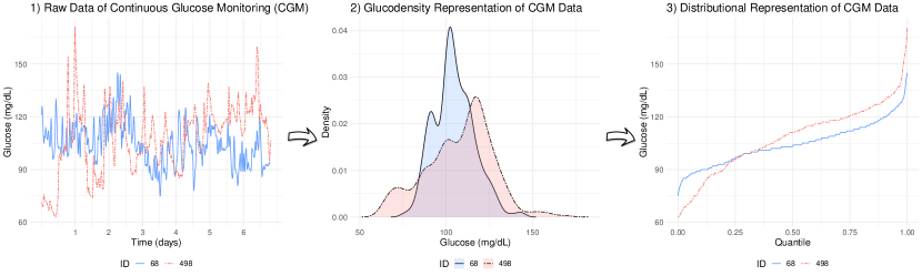
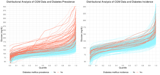
Figure 1: Toprow plots represent the transformation from Continuous Glucose Monitoring (CGM) raw data into glucodensities and its distributional representation. This process is illustrated for two subjects; ID = 498 who was diagnosed of diabetes during follow-up, and a healthy control ID = 68. In the bottom plot we display the distributional representation of CGM data for our sample of subjects differentiating by baseline or follow-up diabetes status.

Figure 1 presents raw continuous glucose monitoring (CGM) data alongside the corresponding glucodensity and its distributional representation for two subjects. Subject 68 serves as a healthy control, while subject 496 developed diabetes in the medium term. While the raw data reveals minimal discernible differences between the individuals, the glucodensity and its distributional representation effectively capture variations in both the mean value and variability of glucose recordings. As we extend our analysis to a larger sample (depicted in the bottom panels of Figure 1), it becomes apparent that the distributional representation of glucodensity may facilitate differentiation between two groups of subjects.

1.2 Optimal cut-points and functional data

The research field of optimal cut points is primarily focused on determining the best values to categorize continuous variables into discrete groups, particularly in the context of diagnostic studies. The clinical relevance of this area of statistical research is evident as it influences how diseases are diagnosed and treated. The estimation of optimal cut points in diagnostic studies encompasses several methodological approaches, each with its theoretical foundations and practical implications. In brief, optimal cut points choice relies on accurately identifying positive and negative cases, which corresponds to sensitivity and specificity. One strategy to obtain a cut point might be based on the maximization of either test’s specificity or sensitivity. However, this procedure proves more extreme, as the choice of an optimal cut point should generally imply an equilibrium between both measures. Notably, Youden’s Index, a widely used method, is referenced in statistical and clinical studies [20, 41], due to its efficacy in maximizing the sum of both sensitivity and specificity to determine the optimal threshold. Receiver Operating Characteristic (ROC) Curve Analysis, extensively discussed in [18], offers a graphical representation of the trade-off between sensitivity and specificity across various cut points, aiding in the selection of the most suitable threshold. Additionally, methods like diagnostic likelihood ratio [7] or cost-effectiveness analysis [39] add up to the statistical toolbox of optimal cut points estimation. To gain a comprehensive understanding and practical implementation of the existing methods for estimating optimal cut points of continuous markers, we recommend consulting Lopez et al.’s work (2014) on this topic [30].

On the other hand the task of categorizing patients using functional data encounters a significant challenge: traditional multivariate analysis techniques, including logistic regression and discriminant analysis, are not directly applicable to functional data due to its infinite-dimensional nature. As a result, a common solution is to modify these multivariate methods for use in functional scenarios, leading to adaptations such as functional logistic regression [1] or functional discriminant analysis [28, 44, 47]. Additional, strategies include the use of kernel methods [19] and support vector machines [46], principal components analysis [26, 22] or functional depth classifiers [11] among others.

In theoretical works, it was proven that perfect classification is feasible for Gaussian functional processes [14, 10] under certain conditions. However, in biomedical problems the classification problems are challenging and there is overlap beetween groups that difficult the perfect clasifications or some close notion to them. This is the case of diabetes, that is heteregoneous and multifactorial disease, that can have different accepted definition according to the medical guidelines that we consider, and universal consensus is not possible about this metabolic disorder.

In this work we extend the field of optimal cut points estimation to the functional data arena. Specifically, we propose a statistical learning model to estimate a functional cut point for classifying subjects based on functional digital biomarkers. The method relies on the distributional representation of the recorded information on which we can estimate a curve discriminating healthy and diseased individuals. Our proposal proved to be reliable with simulated and real world clinical data.

2 Mathematical models

The objective of this section is to introduce a comprehensive framework for determining optimal cut points within statistical objects that take values in arbitrary separable Hilbert spaces, denoted as $\mathcal{H}$. Given our ultimate aim of applying such models to the distributional representation of continuous glucose monitoring (CGM) data, we initiate our discussion by formally defining suchs representations. Subsequently, we present a generalized formulation of an optimal-cut algorithm designed for application in any separable Hilbert spaces. Finally, to exemplify the algorithm’s application, we focus on its implementation within the context of distributional representations derived from CGM data.

2.1 Definition of distributional representation of glucose values: glucodensity

We start with the formal definition of distributional representation of glucose values. For a given patient $i$, we denote the glucose monitoring data by pairs $(t_{ij},X_{ij})$, $j=1,\ldots,m_{i}$, where $t_{ij}$ represents the recording times that are typically equally spaced across the observation interval, while $X_{ij}\in[a,b]$ is the glucose level at time $t_{ij}\in[0,T_{i}]$, where $a$ and $b$ represent the minimum and maximum range of CGM monitor, that in our case $a=40$ mg/dL, and $b=400$ mg/dL. The number of records $m_{i}$, and thus the spacing between them, and the overall observation length $T_{i}$, are allowed to vary across patients. One can see these data as discrete observations of a continuous latent process $Y_{i}(t)$ with $X_{ij}=Y_{i}(t_{ij})$. The glucodensity is defined as $f_{i}(x)=F_{i}^{\prime}(x)$, where $F_{i}^{\prime}(x)$ represents the derivative of the cumulative distribution function $F_{i}(x)$. This distribution function is given by:

$$F_{i}(x)=\frac{1}{T_{i}}\int_{0}^{T_{i}}\mathbb{I}(Y_{i}(t)\leq x)dt$$

for $\underset{t\in[0,T_{i}]}{\inf}Y_{i}(t)\leq x\leq\underset{t\in[0,T_{i}]}{\sup}Y_{i}(t)$.

This expression refers to the proportion of the observational interval in which the glucose level remains below the value $x$. $F_{i}$ are a set of increasing functions from $0$ to $1$. While, for $x\in[a,b]$, $f_{i}(x)$, roughly speaking, measures the proportion of individuals spending time with continuous glucose concentration $x$ over the continuous domain $[a,b]$. Density function modeling is a natural extension of traditional CGM data analysis methods called time-in-range metrics, that measure the proportion of time individuals spend over some range, e.g. hypoglycemia $\widehat{Hipo}_{i}=\frac{1}{n_{i}}\sum_{j=1}^{n_{i}}\mathbf{I}\{X_{ij}\leq 54\}$, but from a functional perspective. From a technical perspective, the use of probability distribution or density functions of the individual CGM time series introduces technical considerations in the statistical analysis because such representations are defined in a metric space without the linear structure of vectorial space. In practice, to overcome such technical difficulties, it is common to consider as representation the quantile function of observed time series, $\widehat{Q}_{i}(\rho)$, that is defined as $\widehat{Q}_{i}(\rho)=\arg\min\{t\in\mathbb{R}:\widehat{F}_{i}(t)=\frac{1}{n_{i}}\sum_{j=1}^{n_{i}}\mathbf{I}\{X_{ij}\leq t\}\geq\rho\}$. Mathematically, in some modeling tasks, it is equivalent to consider the space of univariate probability distribution and density functions equipped with the $2$-Wasserstein distance (see for example [35]).

2.2 Defining Optimal Cut-Points in Separable Hilbert Spaces for Statistical Objects

This section outlines a methodology to determine optimal cut-points for categorizing a response variable $Y$ situated within a separable Hilbert space $\mathcal{H}$. For each subject $i$, let $Z_{i}\in\{0,1\}$ represent a binary indicator of group membership, where $0$ signifies the control (non-disease) group and $1$ signifies the case (disease) group. We introduce a continuous parameter $c$ within a specified range $[e,f]$, to partition the space $\mathcal{H}$ into two regions: $\mathcal{A}^{c+}$ for subjects with a positive condition and $\mathcal{A}^{c-}$ for those without. The classification of an observation $Y_{i}$ into $\mathcal{A}^{c+}$ or $\mathcal{A}^{c-}$ depends on the indicator function $I^{c}_{i}$, which compares against the actual group membership $Z_{i}$. We aim to optimize $c$ by maximizing the following metrics:

Sensitivity $$:\max_{c\in[e,f]}\mathbb{P}(I^{c}_{i}=1|Z_{i}=1),$$

Specificity $$:\max_{c\in[e,f]}\mathbb{P}(I^{c}_{i}=0|Z_{i}=0),$$

Youden Index $$:\max_{c\in[e,f]}\left(\mathbb{P}(I^{c}_{i}=1|Z_{i}=1)+\mathbb{P}(I^{c}_{i}=0|Z_{i}=0)-1\right).$$

To facilitate the partitioning into $\mathcal{A}^{c+}$ and $\mathcal{A}^{c-}$, we define a function $h^{\sigma}_{c}(\rho)$, with $c$ as a real-valued parameter and $\rho$ belonging to the domain $\mathcal{S}$ of $Y$. This function is given by:

$$h^{\sigma}_{c}(\rho)=\mu(\rho)+c\sigma(\rho),\quad\forall\rho\in\mathcal{S},$$

where $\mu=\mathbb{E}(Y)$ denotes the expected mean (or other centrality measures like median or mode could be used), and $\sigma$ represents a scaling function, which, for simplicity, we assume to be constant ($\sigma(\rho)=1$) across all $\rho$ in $\mathcal{S}$ for clinical applications. With a selected $c$, $h^{\sigma}_{c}(\rho)$ helps in defining the regions $\mathcal{A}^{c+}$ and $\mathcal{A}^{c-}$ as follows:

$$\mathcal{A}^{c+}=\{f\in\mathcal{H}:f(\rho)\geq h^{\sigma}_{c}(\rho),\forall\rho\in\mathcal{S}\},\quad\mathcal{A}^{c-}=\{f\in\mathcal{H}:f(\rho)<h^{\sigma}_{c}(\rho),\forall\rho\in\mathcal{S}\}.$$

2.3 Practical Calculation of Optimal Cut Points for CGM Time Series Data

In contexts where $\mathcal{H}$ denotes the space of increasing quantile functions, ranging from $[40,400]$, to reflect the measurement spectrum of Continuous Glucose Monitoring (CGM) devices, we represent the random response for patient $i$ as $Y_{i}(\rho)=\widehat{Q}_{i}(\rho)$, with $\rho\in[0,1]$ signifying the quantile probabilities.

Considering a i.i.d sample $\mathcal{D}_{n}=\{(Y_{i},Z_{i})\sim P\}_{i=1}^{n}$, the function $h^{\sigma}_{c}(\rho)$ for any $c$ value is defined as:

$$h^{\sigma}_{c}(\rho)=\frac{1}{n}\sum_{i=1}^{n}Y_{i}(\rho)+c,$$

enabling the categorization into $\mathcal{A}^{c+}$ and $\mathcal{A}^{c-}$, thereby calculating $I^{c}_{i}$. This facilitates the empirical estimation of sensitivity, specificity, and the Youden Index:

$$\widehat{\text{Sen}}_{c}=\frac{\sum_{i=1}^{n}\mathbb{I}(I^{c}_{i}=1\land Z_{i}=1)}{\sum_{i=1}^{n}\mathbb{I}(Z_{i}=1)},$$

$$\widehat{\text{Spe}}_{c}=\frac{\sum_{i=1}^{n}\mathbb{I}(I^{c}_{i}=0\land Z_{i}=0)}{\sum_{i=1}^{n}\mathbb{I}(Z_{i}=0)},$$

$$\widehat{\text{You}}_{c}=\widehat{\text{Sen}}_{c}+\widehat{\text{Spe}}_{c}-1.$$

By assessing these metrics over a range of $c$ values, $\mathcal{A}=\{c_{1},\ldots,c_{m}\}$, we identify the $c$ that optimizes these criteria based on empirical measures.

2.4 Bootstrapping for Uncertainty Quantification in Optimal Cut-off Determination

Utilizing the dataset $\mathcal{D}_{n}=\{(Y_{i},Z_{i})\}_{i=1}^{n}$, we identify the optimal cut-point $\widehat{c}$, optimizing for sensitivity, specificity, and the Youden Index through a one-dimensional $c$-process, integrating a family of functions:

$$h^{\sigma}_{c}(\rho)=\mu(\rho)+c\sigma(\rho),\quad c\in[e,f].$$

Bootstrap resampling is conducted $B$ times, generating samples $\mathcal{D}^{b}_{n}=\{(Y_{i},Z_{i})\}_{i\in\mathbb{I}_{b}}$ by drawing with replacement from the index set $\mathcal{I}=\{1,\dots,n\}$. This approach yields a series of optimal cut-points $\{\widehat{c}_{b}\}_{b=1}^{B}$. We employ empirical quantiles $\left[\alpha/2,1-\alpha/2\right]$ to calculate confidence intervals, establishing confidence regions for these optimal cut points. This method facilitates inferential analysis on the optimal cut-points within a functional space using bootstrapping.

Theorem 1.

The asymptotic distribution of the estimated optimal cut-point $\widehat{c}$, concerning sensitivity, specificity, and the Youden Index criteria, follows a Gaussian distribution. Consequently, the application of the bootstrap resampling technique for inference is justified.

Proof.

Assuming the functions $\mu$ and $\sigma$ are fixed for simplicity, the regions $\mathcal{A}^{c+}$ exhibit a finite V.C. dimension. This characteristic ensures that the empirical process associated with the $M$-estimator, which maximizes sensitivity, specificity, and the Youden Index, complies with the Donsker principle. Therefore, employing a bootstrapping algorithm with Efron multipliers to construct confidence bands around the estimator $\widehat{c}$ achieves universal consistency due to the guaranteed asymptotic normality. In instances where the functions $\mu$ and $\sigma$ are estimated using the sample data, a data splitting strategy can be applied to simplify the analysis, preserving the bootstrap’s reliability and consistency. ∎

2.5 Computational details

The implementation of this methodology involves the functionalities of two R packages for optimal cutpoint estimation within functional data. First, the fda [45] package is employed to calculate the functional mean, representing the average curve across the provided data. Subsequently, we estimate the maximum value of c at which a given curve is above the functional cutpoint. Subsequently, the optimal.cutpoints package [30] facilitates the core analysis. Specifically, this package calculates a chosen performance metric (e.g., Youden’s Index) over the distribution of the obtained c values. This cutpoint corresponds to the value of c which offer the best performance metric, signifying the ideal separation between classes within the functional data.

3 Simulation study

In this section, we assess the efficacy of our proposal using simulated functional distributional data. The data generating process is based on the following formulation. Given a binary variable $Z\in Ber(0.5)$, and the quantile function $Q_{0}(\rho)$ from a truncate normal distribution $\text{TN}(\mu=1,\sigma^{2}=1,a=-5,b=5)$ the quantile function of the functional distributional records are given by

$$Q(\rho)=aZ+U_{1}+U_{2}v+(5+b)ZU_{3}Q_{0}(\rho)$$ (1)

where $U_{1}\sim U(-1,1)$, $U_{2}\sim U(-1,1)$ and $U_{3}\sim U(0.8,1.2)$. The parameter $v$ was fixed to $v=2$ and it controls the degree of variability along $\rho$ of the simulated curves. The parameter $a$ governs the degree of difference between both groups regarding the location term of distributional functional data. Finally, $b$ is a parameter modulating the degree of difference between both groups due to the variability of the distributional functional data. A sketch of the simulated data is shown in Figure 2 for different values of these parameters.

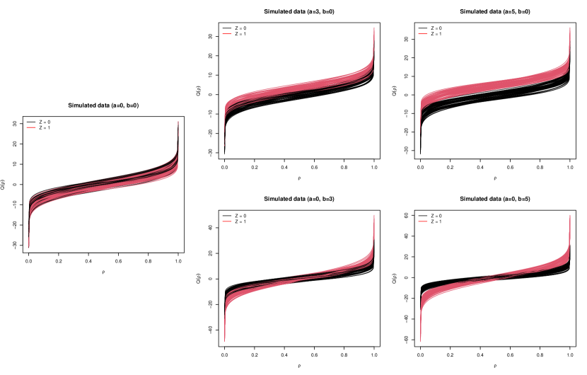
Figure 2: Example of the simulated distributional data for different values of parameters $a$ and $b$, with $n=100$.

In this simulation scenario, we generated data according to equation (1) using various values for parameters $a$ and $b$. Then, we assessed the discrimination capability of the proposed method between both groups. The disparities between the $Z=0$ and $Z=1$ groups are due to variations in either the location parameter (represented by varying $a$) or the scale parameter (represented by varying $b$).

We estimated the functional cutpoint under three criteria: 1) Youden index criteria, 2) maximum sensitivity estimator , and 3) maximum specificity estimator. Sample sizes were set to $n=100$ and $n=1000$. The assessment was carried out across $R=1000$ replicates, with empirical sensitivity and specificity calculated for each classifier in every replicate.

In Figure 3, we present the sensitivity and specificity distribution across different values of $a$ and $b$. The Youden criteria display better performance improvements with increasing values of $a$ or $b$. Notably, the model exhibits the ability to accurately classify subjects regardless of whether the difference stems from location or scale parameters. As sample size increases the variability of the obtained sensitivities and specificities decreases.

On the other hand, the maximum sensitivity criteria consistently yield the highest sensitivity values regardless of the parameter values, while specificity gradually increases with greater disparities between groups. For values of the parameters $a$ and $b$ higher than $3.5$ we observe fair values for specificity. As in the Youden case, a higher sample size reduces the variability of the estimated specificities. Conversely, the maximum specificity criteria exhibit an inverse trend, showing a fair sensitivity for $a$ or $b$ values higher than 3.5. Finally, the sensitivity variability decreases as sample size becomes higher. Both maximum sensitivity and specificity criteria works well with independence if the groups show differences on location or scale parameters.

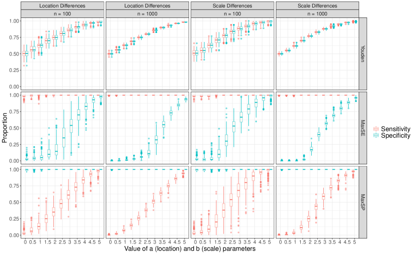
Figure 3: Simulation results: estimated sensitivities and specificities for optimal cutoff curves based on Youden’s, maximum specificity, and maximum sensitivity criteria across varying sample sizes and differences in location and scale parameters between groups.

4 Clinical validation of the optimal functional cutpoint

In this section, we apply the proposed methodology to classify individuals into two groups based on their diabetes status, using continuous glucose monitoring (CGM) records as the primary data source. Our first objective is to identify individuals currently experiencing anomalies in glycemic regulation. Our second objective is to identify individuals who face an increased risk of developing diabetes in the medium term.

The data source for this study is the A-Estrada Glycation and Inflammation Study, a population-based research project in which 580 participants underwent CGM during a week ten years ago. Currently, health events are being recorded based on electronic health records (EHRs).

4.1 AEGIS project

The present study comprises a subsample of subjects from the A Estrada Glycation and Inflammation Study (AEGIS; trial NCT01796184 at www.clinicaltrials.gov). AEGIS is a cross-sectional population study of adults (aged $\geq$ 18) from a Spanish municipality. A detailed description of AEGIS can be found in Gude et al., (2017)[25].

In AEGIS, participants were periodically examined at their primary care center for one year, beginning in March. During these visits, participants completed an interviewer-administered structured questionnaire, provided a lifestyle description, underwent biochemical measurements, and were prepared for continuous glucose monitoring (CGM).

From 1516 subjects enrolled in the AEGIS project, 622 participants consented to undergo a CGM. Moreover, those subjects accepted to writting down their meal intake into a diary. From this sample, 5 did not fulfilled the study protocol and 37 experienced a disconnection of the biosensor during the monitoring period. Therefore, we count with 580 participants (360 women, 220 men) who completed at least two days of CGM. Of those, 65 subjects suffered from diabetes.

At the start of each monitoring period, a research nurse inserted an Enlite^TM continuous glucose monitoring (CGM) sensor (Medtronic, Inc., Northridge, CA, USA) subcutaneously into the subject’s abdomen. The sensor continuously measured the interstitial glucose level (40-400 mg/dL) of the subcutaneous tissue, recording values every 5 minutes. Participants were also provided with a conventional OneTouchR VerioR Pro glucometer (LifeScan, Milpitas, CA, USA) as well as compatible lancets and test strips for calibrating the CGM. All subjects were asked to make at least three capillary blood glucose measurements (usually before the main meals) without checking the current CGM reading. The sensor was removed on the seventh day, and the data was downloaded and stored for further analysis. If the total number of data acquisition skips per day exceeded 2 hours, all of the data for that day was discarded.

During the following years monitored individuals were followed using their electronic health records. Based on periodic blood test ordered by their primary care doctor we could identify which subjects developed the disease. A participant was considered to have or developed diabetes if they met either of the following criteria (as given by the American Diabetes Association):

1. A glycated hemoglobin level above 6.5% and a fasting plasma glucose level of 126 mg/dL or higher in a single blood test.

2. One of these criteria above the diagnostic cut points in two separate blood tests.

4.2 Optimal functional cutpoint estimation

From the 580 subjects 65 was previously diagnosed with diabetes which corresponds to a prevalence of $11.2\%$ $($CI95$\%$: $3.8\%-14.1\%))$. By August 2022, the diabetes status of all participants was checked based on their electronic health records. From 515 subjects showing no diabetes at baseline, $26$ (incidence rate = $5.0\%$ (CI$95\%$: $3.4\%-7.4\%$) developed the disease during the follow-up.

Optimal cut-off curves for maximum sensitivity, Youden index and maximum specificity criteria are depicted in Figure 4 for predicting cases of diabetes prevalence and incidence. Alongside the estimated curve we present their corresponding $95\%$ pointwise confidence bands.

Firstly, for predicting diabetes prevalence maximum sensitivity criteria offer poor specificity $0.15$ (CI$95\%:0.12-0.68$). The median glucose value for this cutoff is $108.2$ mg/dL, spending $\geq 4.0\%$ time above the 140 mg/dL threshold. The Youden criteria shows a good balance between sensitivity and specificity being $0.89$ (CI$95\%:0.85-0.92$) for both quantities. The median value of this cutoff curve rises until $135.9$ mg/dL, so does time above 140 mg/dL which increases until $\geq 38.2\%$. Finally, maximum specificity cut-off curve show a low sensitivity of $0.51$ (CI$95\%:0.43-0.60$). The median value rises until $201.8$ mg/dL, and the curve is above 140 mg/dL along the domain function. This curve identify subjects who reach very high glucose excursion a low proportion of time.

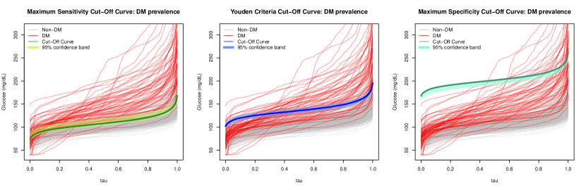
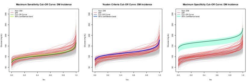
Figure 4: Optimal cut-off curves for predicting diabetes prevalence and incidence alongside with 95% pointwise confidence band. The confidence band was obtained using 1000 uniform bootstrap replicates.

On the other hand, when predicting diabetes incidence, criteria based on maximum sensitivity exhibit poor specificity ($0.19$, 95% CI: $0.14$ - $0.46$). The median glucose value for this cutoff curve is $106.2$ mg/dL, with $\geq 3.1\%$ of time spent above the 140 mg/dL threshold. In contrast, the Youden criteria demonstrates a balanced trade-off between sensitivity and specificity, yielding $0.69$ (95% CI: $0.62$ - $0.73$) for both metrics. The median value of this cutoff curve increases until reaching $118.8$ mg/dL, with time spent above 140 mg/dL also increasing to $\geq 9.5$%. Conversely, the curve for maximum specificity cut-off demonstrates a very low sensitivity ($0.06$, 95% CI: $0.04$ - $0.08$). Its median value rises until $174.7$ mg/dL, remaining above the 140 mg/dL threshold throughout.

As depicted in Figure 5 the estimated cutoff curves show higher discrimination for diabetes prevalence than for diabetes incidence. When we considered the specificities and (1-sensitivities) for the entire range of $c$ we obtain the depicted ROC curves. As can be seen, while the prediction of diabetes prevalence shows an AUC of $0.94$ (CI$95\%:0.90-0.95$), the prediction of future development of the disease show a lower area under the curve of $0.78$ (CI$95\%:0.68-0.80$).

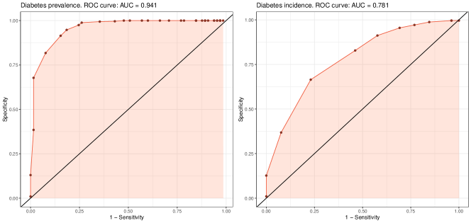
Figure 5: ROC curves, depicting specificities vs. (1 - sensitivities), obtained for a varying value of $c$ in the functional cut-point. Left plot shows the discrimination capability of the functional-cutpoint for diabetes prevalence, while right plot focus on predicting diabetes incidence.

5 Discussion

This paper proposes a new methodology for defining optimal cut points for statistical objects within a separable Hilbert space. The method’s reliability is demonstrated using both simulated and real-world data. We applied the method to a clinical problem: classifying patients based on digital biomarkers obtained from continuous glucose monitoring. This allowed us to identify prevalent cases of diabetes and to predict the incidence of the disease. The method exhibited excellent discrimination capability, and for the first time, we were able to determine various functional cut-points that balanced sensitivity and specificity. Additionally, we estimated a 95% confidence band to quantify the uncertainty associated with the cut-point estimation.

Our findings hold significant relevance for diabetes mellitus research. Continuous glucose monitoring (CGM) data is increasingly playing a key role in diagnosis and disease management, potentially leading to improved diagnostic criteria and treatment protocols [4]. A statistical model that get advantage of CGM data to formulate a classification rule for diabetes would serve as a valuable practical resource. Existing research has identified individuals at higher risk of developing diabetes based on metrics like time spent above a certain blood sugar range [31]. Additionally, studies have shown changes in CGM glucodensity with aging [40]. Notably, our work presents the first evidence that distributional representations of glucodensity can be instrumental in early diagnosis of diabetes. Integrating this interpretable graphical rule into CGM software would be highly beneficial for both clinicians and the CGM industry.

Finally, the applications of this statistical methodology may be extended broadly across the biomedical field. It can be used to define interpretable decision rules in clinical trials involving continuous subject monitoring [5], or in the context of digital health [49]. As wearable devices become increasingly prevalent for disease characterization, our methodology has the potential to be instrumental in defining new metabolic states of patients or diseases. Furthermore, this framework can be potentially applied to other domains, such as neuroimaging, where data can be represented by Laplacian graphs embedded in a separable Hilbert space.

References

- [1] Yuko Araki, Sadanori Konishi, Shuichi Kawano, and Hidetoshi Matsui. Functional logistic discrimination via regularized basis expansions. Communications in Statistics-Theory and Methods, 38(16-17):2944–2957, 2009.
- [2] Lmar M Babrak, Joseph Menetski, Michael Rebhan, Giovanni Nisato, Marc Zinggeler, Noé Brasier, Katja Baerenfaller, Thomas Brenzikofer, Laurenz Baltzer, Christian Vogler, et al. Traditional and digital biomarkers: two worlds apart? Digital biomarkers, 3(2):92–102, 2019.
- [3] Tadej Battelino, Thomas Danne, Richard M Bergenstal, Stephanie A Amiel, Roy Beck, Torben Biester, Emanuele Bosi, Bruce A Buckingham, William T Cefalu, Kelly L Close, et al. Clinical targets for continuous glucose monitoring data interpretation: recommendations from the international consensus on time in range. Diabetes care, 42(8):1593–1603, 2019.
- [4] Pilar Isabel Beato-Víbora, Ana Chico, Jesus Moreno-Fernandez, Virginia Bellido-Castañeda, Lia Nattero-Chávez, María José Picón-César, María Asunción Martínez-Brocca, Marga Giménez-Álvarez, Eva Aguilera-Hurtado, Elisenda Climent-Biescas, et al. A multicenter prospective evaluation of the benefits of two advanced hybrid closed-loop systems in glucose control and patient-reported outcomes in a real-world setting. Diabetes Care, 47(2):216–224, 2024.
- [5] Ulrikke Lyng Beauchamp, Helle Pappot, and Cecilie Holländer-Mieritz. The use of wearables in clinical trials during cancer treatment: systematic review. JMIR mHealth and uHealth, 8(11):e22006, 2020.
- [6] Roy W Beck, Richard M Bergenstal, Tonya D Riddlesworth, Craig Kollman, Zhaomian Li, Adam S Brown, and Kelly L Close. Validation of time in range as an outcome measure for diabetes clinical trials. Diabetes care, 42(3):400–405, 2019.
- [7] Edward J Boyko. Ruling out or ruling in disease with the most sensitiue or specific diagnostic test: Short cut or wrong turn? Medical Decision Making, 14(2):175–179, 1994.
- [8] Jennifer A Bunn, James W Navalta, Charles J Fountaine, and Joel D Reece. Current state of commercial wearable technology in physical activity monitoring 2015–2017. International journal of exercise science, 11(7):503, 2018.
- [9] Xiangmao Chang, Gangkai Li, Guoliang Xing, Kun Zhu, and Linlin Tu. Deepheart: A deep learning approach for accurate heart rate estimation from ppg signals. ACM Transactions on Sensor Networks (TOSN), 17(2):1–18, 2021.
- [10] Juan Cuesta-Albertos and Subhajit Dutta. On perfect clustering for gaussian processes. Transactions on Machine Learning Research, 2023.
- [11] Antonio Cuevas, Manuel Febrero, and Ricardo Fraiman. Robust estimation and classification for functional data via projection-based depth notions. Computational Statistics, 22(3):481–496, 2007.
- [12] Elvis Han Cui, Allison B Goldfine, Michelle Quinlan, David A James, and Oleksandr Sverdlov. Investigating the value of glucodensity analysis of continuous glucose monitoring data in type 1 diabetes: an exploratory analysis. Frontiers in Clinical Diabetes and Healthcare, 4, 2023.
- [13] Bruce Del Mar. The history of clinical holter monitoring. Annals of noninvasive electrocardiology: the official journal of the International Society for Holter and Noninvasive Electrocardiology, Inc, 10(2):226, 2005.
- [14] Aurore Delaigle and Peter Hall. Achieving near perfect classification for functional data. Journal of the Royal Statistical Society Series B: Statistical Methodology, 74(2):267–286, 2012.
- [15] Andrew Downs, Jacqueline Van Hoomissen, Andrew Lafrenz, and Deana L Julka. Accelerometer-measured versus self-reported physical activity in college students: Implications for research and practice. Journal of American College Health, 62(3):204–212, 2014.
- [16] Monica M Dua, Anand Navalgund, Steve Axelrod, Lindsay Axelrod, Patrick J Worth, Jeffrey A Norton, George A Poultsides, George Triadafilopoulos, and Brendan C Visser. Monitoring gastric myoelectric activity after pancreaticoduodenectomy for diet “readiness”. American Journal of Physiology-Gastrointestinal and Liver Physiology, 315(5):G743–G751, 2018.
- [17] Jessilyn Dunn, Ryan Runge, and Michael Snyder. Wearables and the medical revolution. Personalized medicine, 15(5):429–448, 2018.
- [18] Tom Fawcett. An introduction to roc analysis. Pattern recognition letters, 27(8):861–874, 2006.
- [19] Frédéric Ferraty and Philippe Vieu. Curves discrimination: a nonparametric functional approach. Computational Statistics & Data Analysis, 44(1-2):161–173, 2003.
- [20] Ronen Fluss, David Faraggi, and Benjamin Reiser. Estimation of the youden index and its associated cutoff point. Biometrical Journal: Journal of Mathematical Methods in Biosciences, 47(4):458–472, 2005.
- [21] Claudio Gentili, Gaetano Valenza, Mimma Nardelli, Antonio Lanatà, Gilles Bertschy, Luisa Weiner, Mauro Mauri, Enzo Pasquale Scilingo, and Pietro Pietrini. Longitudinal monitoring of heartbeat dynamics predicts mood changes in bipolar patients: A pilot study. Journal of affective disorders, 209:30–38, 2017.
- [22] Richard H Glendinning and RA Herbert. Shape classification using smooth principal components. Pattern recognition letters, 24(12):2021–2030, 2003.
- [23] Fernando Gomez-Peralta, Ana Chico Ballesteros, Amparo Marco Martínez, Begoña Pérez Corral, Ignacio Conget Donlo, Paulina Fuentealba Melo, Fernando Zaragozá Arnáez, and Marcos Matabuena Rodríguez. Insulin glargine 300 u/ml versus insulin degludec 100 u/ml improves nocturnal glycaemic control and variability in type 1 diabetes under routine clinical practice: A glucodensities-based post hoc analysis of the onecare study. Diabetes, Obesity and Metabolism, 2024.
- [24] Juvenile Diabetes Research Foundation Continuous Glucose Monitoring Study Group. Continuous glucose monitoring and intensive treatment of type 1 diabetes. New England Journal of Medicine, 359(14):1464–1476, 2008.
- [25] Francisco Gude, Pablo Díaz-Vidal, Cintia Rúa-Pérez, Manuela Alonso-Sampedro, Carmen Fernández-Merino, Jesús Rey-García, Carmen Cadarso-Suárez, Marcos Pazos-Couselo, José Manuel García-López, and Arturo Gonzalez-Quintela. Glycemic variability and its association with demographics and lifestyles in a general adult population. Journal of diabetes science and technology, 11(4):780–790, 2017.
- [26] Peter Hall, Donald S Poskitt, and Brett Presnell. A functional data—analytic approach to signal discrimination. Technometrics, 43(1):1–9, 2001.
- [27] Apple Inc. Healthkit, 2023. Accessed: 2023-08-31.
- [28] Gareth M James and Trevor J Hastie. Functional linear discriminant analysis for irregularly sampled curves. Journal of the Royal Statistical Society Series B: Statistical Methodology, 63(3):533–550, 2001.
- [29] Stephen P Lee, Grace Ha, Don E Wright, Yinji Ma, Ellora Sen-Gupta, Natalie R Haubrich, Paul C Branche, Weihua Li, Gilbert L Huppert, Matthew Johnson, et al. Highly flexible, wearable, and disposable cardiac biosensors for remote and ambulatory monitoring. NPJ digital medicine, 1(1):2, 2018.
- [30] Mónica López-Ratón, María Xosé Rodríguez-Álvarez, Carmen Cadarso-Suárez, and Francisco Gude-Sampedro. Optimalcutpoints: an r package for selecting optimal cutpoints in diagnostic tests. Journal of statistical software, 61:1–36, 2014.
- [31] Alejandra Marco, Marcos Pazos-Couselo, Jesús Moreno-Fernandez, Ana Díez-Fernández, Manuela Alonso-Sampedro, Carmen Fernández-Merino, Arturo Gonzalez-Quintela, and Francisco Gude. Time above range for predicting the development of type 2 diabetes. Frontiers in Public Health, 10:1005513, 2022.
- [32] Marcos Matabuena and Ciprian M. Crainiceanu. Multilevel functional distributional models with application to continuous glucose monitoring in diabetes clinical trials, 2024.
- [33] Marcos Matabuena, Paulo Felix, Carlos Garcia-Meixide, and Francisco Gude. Kernel machine learning methods to handle missing responses with complex predictors. application in modelling five-year glucose changes using distributional representations. Computer Methods and Programs in Biomedicine, 221:106905, 2022.
- [34] Marcos Matabuena and Alexander Petersen. Distributional data analysis of accelerometer data from the nhanes database using nonparametric survey regression models. Journal of the Royal Statistical Society Series C: Applied Statistics, 72(2):294–313, 2023.
- [35] Marcos Matabuena, Alexander Petersen, Juan C Vidal, and Francisco Gude. Glucodensities: A new representation of glucose profiles using distributional data analysis. Statistical methods in medical research, 30(6):1445–1464, 2021.
- [36] Sven Meister, Wolfgang Deiters, and Stefan Becker. Digital health and digital biomarkers–enabling value chains on health data. Current Directions in Biomedical Engineering, 2(1):577–581, 2016.
- [37] Megan C Nelson, Katie Taylor, and Chantal A Vella. Comparison of self-reported and objectively measured sedentary behavior and physical activity in undergraduate students. Measurement in Physical Education and Exercise Science, 23(3):237–248, 2019.
- [38] Michelle Nguyen, Julia Han, Elias K Spanakis, Boris P Kovatchev, and David C Klonoff. A review of continuous glucose monitoring-based composite metrics for glycemic control. Diabetes technology & therapeutics, 22(8):613–622, 2020.
- [39] Rex Parsons, Robin Blythe, Susanna M Cramb, and Steven M McPhail. Integrating economic considerations into cutpoint selection may help align clinical decision support toward value-based healthcare. Journal of the American Medical Informatics Association, 30(6):1103–1113, 2023.
- [40] Marcos Pazos-Couselo, Cristina Portos-Regueiro, María González-Rodríguez, Jose Manuel García-Lopez, Manuela Alonso-Sampredro, Raquel Rodríguez-González, Carmen Fernández-Merino, and Francisco Gude. Aging of glucose profiles in an adult population without diabetes. Diabetes research and clinical practice, 188:109929, 2022.
- [41] Neil J Perkins and Enrique F Schisterman. The inconsistency of “optimal” cutpoints obtained using two criteria based on the receiver operating characteristic curve. American journal of epidemiology, 163(7):670–675, 2006.
- [42] Leonardo Zumerkorn Pipek, Rafaela Farias Vidigal Nascimento, Milena Marques Pagliarelli Acencio, and Lisete Ribeiro Teixeira. Comparison of spo2 and heart rate values on apple watch and conventional commercial oximeters devices in patients with lung disease. Scientific Reports, 11(1):18901, 2021.
- [43] Nalinee Poolsup, Naeti Suksomboon, and Aye Mon Kyaw. Systematic review and meta-analysis of the effectiveness of continuous glucose monitoring (cgm) on glucose control in diabetes. Diabetology & metabolic syndrome, 5:1–14, 2013.
- [44] Cristian Preda, Gilbert Saporta, and Caroline Lévéder. Pls classification of functional data. Computational Statistics, 22(2):223–235, 2007.
- [45] J. O. Ramsay, Spencer Graves, and Giles Hooker. fda: Functional Data Analysis, 2022. R package version 6.0.5.
- [46] Fabrice Rossi and Nathalie Villa. Support vector machine for functional data classification. Neurocomputing, 69(7-9):730–742, 2006.
- [47] Hyejin Shin. An extension of fisher’s discriminant analysis for stochastic processes. Journal of Multivariate Analysis, 99(6):1191–1216, 2008.
- [48] Emese Sükei, Santiago de Leon-Martinez, Pablo M Olmos, and Antonio Artés. Automatic patient functionality assessment from multimodal data using deep learning techniques–development and feasibility evaluation. Internet Interventions, page 100657, 2023.
- [49] Jiaobing Tu, Rebeca M Torrente-Rodríguez, Minqiang Wang, and Wei Gao. The era of digital health: A review of portable and wearable affinity biosensors. Advanced Functional Materials, 30(29):1906713, 2020.
- [50] Wilbert Villena Gonzales, Ahmed Toaha Mobashsher, and Amin Abbosh. The progress of glucose monitoring—a review of invasive to minimally and non-invasive techniques, devices and sensors. Sensors, 19(4):800, 2019.