Revisiting the barometric equation and the extent of a planetary atmosphere

Abstract

The standard barometric equation predicts the molecular concentration $n(z)=n_{0}\exp(-z/L)$ where $L=k_{B}T/mg$. Because the mean free path $l=1/n\sigma$ increases exponentially, we show that at high altitudes $z$, the equation is no longer within the domain of applicability of the standard kinetic theory $l\ll L$. Here, we predict the dependence $n(z)\propto z^{-2}$ for the case $l\gg L$ in uniform gravity. It corresponds to a non-stationary planetary atmosphere with hydrogen accretion. The predicted accretion is accompanied by a release of gravitational potential energy that leads to heating of the atmosphere. In that context, we suggest gravitational energy could be the elusive source that drives the formation of stellar coronas. Other consequences of accretion are: slowly decaying tails of planetary atmospheres, the existence of gas giants, and periodical hydrogen explosions of white dwarfs.

I Barometric equation

The barometric equation,

$$n(z)=n_{0}\exp\left(-\frac{z}{L}\right)\quad{\rm with}\quad L=\frac{k_{B}T}{mg}$$ (1)

follows from the Boltzmann-Gibbs distribution $n=n_{0}\exp[-U(z)/k_{B}T]$ with the potential energy $U=mgz$ and can be expressed in terms of pressure $P=nk_{B}T$. While this approach does not invoke the mean free path $l$ or other kinetic concepts, it is limited to the condition of gas theory, $l\ll L$.

The latter limitation becomes more explicit when we present a derivation based on the kinetic concepts based on the stationary continuity equation,

$$-D\frac{dn}{dz}+vn=0.$$ (2)

For the diffusion coefficient, we use the standard approximation,

$$D=v_{T}l=v_{T}/(n\sigma)\quad{\rm with}\quad v_{T}=\sqrt{k_{B}T/m},$$ (3)

where $v_{T}$ is the thermal velocity and $\sigma$ is the cross section of molecular interactions. The drift velocity $v=\mu F$ with $\mu$ being the mobility and $F=-mg$ force according to the Einstein relation, $\mu=D/k_{B}T$. Eq. (2) reduces then to the differential equation $Ddn/dz+(D/k_{b}T)mgn=0$ yielding the barometric formula.

We now express the criterion $l\ll L$ through gas parameters: [1]

$$\frac{k_{B}T}{mgl}\gg 1.$$ (4)

Another form of the same is expressed through the temperature limitation, [1]

$$T>T_{g}\equiv\frac{mgl}{k_{B}}.$$ (5)

Whichever of the two is used, that criterion can be interpreted as a limitation on gas concentration $n$ that must be high enough for the barometric equation to apply. Introducing zero altitude mean free path $l_{0}=1/n_{0}\sigma$, an approximate formula for the upper bound domain for, barometric formula region is given by,

$$z=z_{c}\approx L\ln\left(\frac{L}{l_{0}}\right).$$ (6)

Its corresponding concentration is roughly estimated as,

$$n_{c}=n_{0}\exp(-z_{c}/L)\approx n_{0}(l_{0}/L).$$ (7)

To keep links with a specific Earth parameters, we refer to the hydrogen, noting $n_{0}\sim 10^{14}$ cm^-3, $\sigma\sim 10^{-16}$ cm², $g=10^{3}$ cm/s², $m\approx 3\times 10^{-24}$ g, thus, Table 1.

Table 1: Some parameters of the Earth hydrogen atmosphere .

parameter	$l_{0}$	$L$	$z_{c}$	$n_{0}$	$n_{c}$
estimate	1 m	120 km	1500 km	$10^{14}$ cm-3	$10^{7}$ cm-3

The domain of lower concentrations at $z>z_{c}$ belongs in the rarified systems. In Sec. III below, we modify our derivation for the case of rarified gases at $z>z_{c}$ where the criteria in Eqs. (4), (5) fail. That alternative domain description should match that of the standard barometric equation when $z=z_{c}$.

II Instability in barometric distribution

Here, we present an evidence of an instability in the Barometric equation. We proceed from the kinetic Boltzmann equation for a one-component gas singlet distribution function $f_{j}^{(1)}({\bf r},{\bf v}_{j},t)$, omitting index $j$ and assuming the hydrogen gas as the lightest,

$$\frac{\partial f^{(1)}}{\partial t}+v\frac{\partial f^{(1)}}{\partial z}-g\frac{\partial f^{(1)}}{\partial v}=I,$$ (8)

$\int dzdvf^{(1)}$ gives the total number of particles. In the relaxation time approximation, the collision integral $I$ is represented as

$$I=-\frac{\delta f}{\tau},\quad{\rm with}\quad\delta f=f^{(1)}-f_{0}^{(1)}$$ (9)

where

$$f_{0}^{(1)}=const\times\exp\left(-\frac{mv^{2}}{2k_{B}T}-\frac{mgz}{k_{B}T}\right)$$ (10)

is the equilibrium distribution function satisfying Eq. (8) with $\partial f/\partial t=0$, $T=const$ and $I=0$. [3, 4, 5]

We seek instabilities of the distribution function, in the form,

$$\delta f=\tilde{f}(t,z)\exp(-mv^{2}/2k_{B}T),$$ (11)

which reduces Eq. (8) to the following.

$$\frac{\partial\tilde{f}}{\partial t}+v\frac{\partial\tilde{f}}{\partial z}-g\frac{mv}{T}\tilde{f}=-\frac{\tilde{f}}{\tau}$$ (12)

Following the standard stability analysis we look for its solution as a Fourier expansion,

$$\tilde{f}=\sum_{\omega,q}a_{\omega,q}^{(0)}\exp(-i\omega t-iqz)$$ (13)

where $\omega$ and $q$ are the frequency and wave number of a partial wave with the initial ($t=0$) amplitude $a_{\omega,q}^{(0)}$. Substituting Eq. (13) into Eq. (12) can result in some partial waves having the positive real parts of $\-i\omega$, i. e. $\Re{(-i\omega)}\equiv\lambda>0$; such a wave is indicative of temporal instability of such waves.

Substituting the ansatz of Eq. (11) into Eq. (12) yields the dispersion law,

$$-i\omega=\frac{mgv}{k_{B}T}-\frac{1}{\tau}+ivk\quad{\rm i.e.}\quad\lambda=\frac{mgv}{k_{B}T}-\frac{1}{\tau}.$$ (14)

The instability criterion $\lambda>0$ takes the form

$$\frac{mgl}{k_{B}T}>1$$ (15)

where $l=v\tau$ is the mean-free-path. It coincides with our former result in Eq. (4). The complementary part of spectrum with $\lambda<0$ represents decaying fluctuations of no interest here. Note that the above instability is related to the term $\partial f^{(1)}/\partial v$ describing the evolution of velocity distribution (across the atmosphere) accounted for by the Boltzmann equation (12).

One additional observation is that the system remains stable for low altitudes ($l$ small enough to keep $\lambda<0$), however it becomes progressively unstable with $z\gg z_{c}$. This corresponds to the downward stream of molecules towards the edge of stability $z_{c}$, the conclusion is of importance for applications addressed in Sec. V.

III Modification for rarified gases

In a dilute gas most of the molecules are not interacting with any other molecule and are just travelling along between collisions. Because of this, the macroscopic behavior of a gas depends only upon a singlet distribution function $f_{j}^{(1)}({\bf r},{\bf v}_{j},t)$ where the subscript $j$ denotes the singlet distribution function of species $j$. One could, if helpful, treat a gas as pure H₂. At about $z\approx 100$ km the numerical density of H₂ is approximately equal to the density of N₂. At $z\approx 200$ km the H₂ density is already $10^{5}$ higher than that of N₂.

Following [2] (p. 406) we introduce the mass average (stream) velocity,

$${\bf v}_{0}({\bf r},t)=\frac{\sum_{j}m_{j}n_{j}{\bf v}_{j}}{\sum_{j}m_{j}n_{j}}$$ (16)

The momentum density of the gas is the same as if all the molecules were moving with velocity ${\bf v}_{0}$.

We define the velocity ${\bf V}_{j}$ of a molecule relative to the stream velocity,

$${\bf V}_{j}={\bf v}_{j}-{\bf v}_{0}.$$ (17)

The average of this peculiar velocity is the diffusion velocity,

$${\overline{\bf V}}_{j}=\frac{1}{n_{i}}\int({\bf v}_{j}-{\bf v}_{0})f_{j}^{(1)}({\bf r},{\bf p}_{j},t)d{\bf v}_{j}.$$ (18)

Its average over all species is zero, $\sum_{j}m_{j}n_{j}{\overline{\bf V}}_{j}=0$.

Due to its stochasticity, the characteristic rms value of ${\overline{\bf V}}_{j}$ can be identified as the thermal velocity,

$$\sqrt{\langle({\overline{\bf V}}_{j})^{2}\rangle}=v_{T}=\sqrt{k_{B}T/m}$$ (19)

where $T$ is treated as the empirical parameter. Therefore, for the diffusion coefficient, we use the standard approximation,

$$D=v_{T}/(n\sigma)\equiv v_{T}l.$$ (20)

On the other hand, the stream velocity $v$ is dominated by the gravity and its average value, specifying the general concept of ${\bf v}_{0}$, is given by

$$v_{0}=v_{g}=\sqrt{gl/2}.$$ (21)

The concept of mobility and its corresponding Einstein relation become irrelevant here. (This is not to say that the velocities of individual molecules in the stream direction are all the same.)

Note that Eq. (21) tacitly assumes zero constant velocity $v_{0}$ in the general expression for accelerated motion, $v=v_{0}+\sqrt{gl/2}$, hence, acceleration starting on average with zero initial velocity after each collision. According to our classification, the random collision-related contributions must be assigned to peculiar velocities; hence, $v_{0}\equiv\langle v_{0}\rangle=0$. The latter appears intuitively obvious because the average momentum change is zero in every pair collision.

Noting that $p_{g}=mv_{g}$ is the stream component of the momentum of one molecule, it is straightforward to see that its related momentum flux

$${\cal P}=(nv_{g})p=mnv_{g}^{2}$$ (22)

remains constant as a function of coordinate because $v_{g}\propto 1/\sqrt{n}$.

It may be important to estimate the corresponding energy flux $\Phi=(nv_{g})(mv_{g}^{2}/2)=(mg/4\sigma)\sqrt{g/2n\sigma}$. Substituting here $n=n_{c}$ from Eq. (7) yields an estimate for the total power per area brought to the gas by the hydrogen accreation,

$$w=\frac{mg}{4\sigma}\sqrt{\frac{gL}{2}}.$$ (23)

Substituting here the above mentioned Earth parameters, yields a numerical estimate, $w\sim 0.1$ $\mu$W/cm² .

With Eqs. (20) and (21) in mind, the continuity equation takes the form,

$$\frac{v_{T}}{n\sigma}\frac{dn}{dz}+\sqrt{\frac{g}{n\sigma}}n=0.$$ (24)

Integrating the latter yields

$$n=\left[n_{c}^{-1/2}+(\sqrt{g\sigma}/2\sqrt{2}v_{T})(z-z_{c})\right]^{-2}.$$ (25)

We observe that the characteristic exponential dependence of the standard barometric equation does not exist for dilute gases. In the deep rarified region of $z\gg z_{c}$, the dependence in Eq. (25) reduces to the form,

$$n=\frac{8k_{B}T}{mg\sigma}\frac{1}{z^{2}}.$$ (26)

Note that Eq. (26) predicts indeed $n\sim n_{c}$ as should be expected from the adopted algorithm of matching the solutions in the barometric equation and the rarified gas regions.

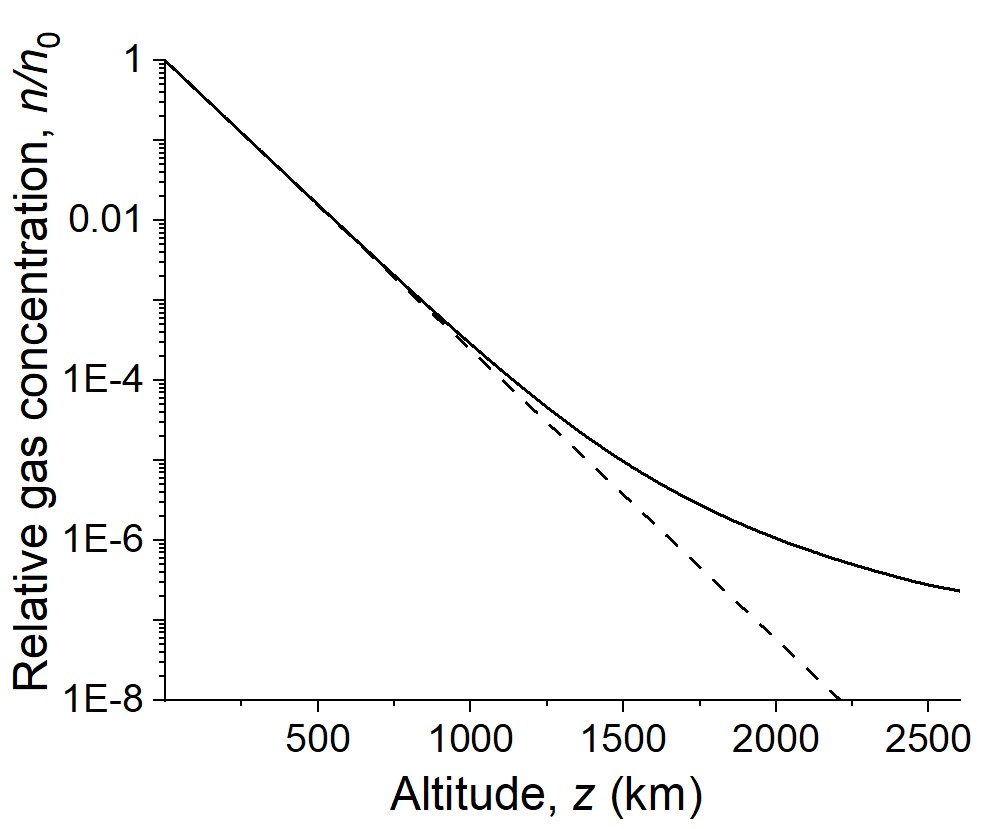
Figure 1: Predicted distributions of the atmosphere density according to arguments of this section. The solid curve presents Eq. (28) with the following numerical parameters: $k_{B}T/mg=120$ km, $\sqrt{mg/k_{B}T\sigma n_{0}}=0.003$. The dashed line represents the barometric formula approximation.

A semiquantitative formula interpolating between the limits of $z\ll z_{c}$ and $z\gg z_{c}$ regions can be obtained by using a convenient approximation for $v$

$$v=v_{T}v_{g}(v_{T}+v_{g})^{-1}$$ (27)

instead of Eq. (21) in the continuity equation. Integrating the latter yields,

$$\ln\left(\frac{n}{n_{0}}\right)-2\sqrt{\frac{mg}{k_{B}T\sigma}}\left(\frac{1}{\sqrt{n}}-\frac{1}{\sqrt{n_{0}}}\right)=-\frac{zmg}{k_{B}T}.$$ (28)

Its predicted dependence is illustrated in Fig. 1. We observe the extended atmosphere tail in the rarified gas domain extending far beyond the barometric formula predictions.

IV Long range behavior

We now consider some predictions related to the gravity being a function of coordinates for the case of a spherically symmetric celestial body of radius $R$. Taking into account the gravity universal law, the above equations remain applicable with the renormalization

$$g\rightarrow g\left(\frac{R_{0}}{R}\right)^{2}$$ (29)

where $R_{0}$ is the planet radius, and $R=R_{0}+z$ is the distance to its center. With the renormalization of Eq. (29) we obtain from Eq.(24),

$$\sqrt{\frac{v_{T}^{2}}{\sigma g}}\frac{dn}{n^{3/2}}=-\frac{R_{0}dR}{R}\quad{\rm when}\quad R\gg R_{0}$$ (30)

where $g$ is the standard acceleration due to gravity at the celestial body surface. Eq. (30) is readily integrated to yield

$$n=n_{0}\left[1+\Lambda\ln(R/R_{0})\right]^{-2}\quad{\rm when}\quad R\gg R_{0}.$$ (31)

Here we have introduced,

$$\Lambda=\sqrt{\frac{n_{0}\sigma mgR_{0}^{2}}{k_{B}T}}\sim 10^{4}-10^{5}.$$ (32)

Again, $g$ remains the acceleration due to gravity at the planet surface, and we assumed the following Earth related numerical values: $n_{0}\sim 10^{14}$ 1/cm³, $T\sim 300-3000$ K,[6] $\sigma\sim 10^{-16}$cm²,[7] $R_{0}=6000$ km, $m=3\times 10^{-24}$ g.

In Fig. 2 we have plotted atmospheric density vs $R/R_{0}$ where the full line is the barometric equation, the dashed line is Eq. (31) with $\Lambda=10^{5}$, and the symbols are values extracted from the published data [8, 6, 9, 10]. The most notable feature in In Fig. 2 is that the dramatic change in slope in the density profile is consistent with experimental data. The latter reflects a qualitatively new situation that emerges when $R_{0}\gg L$: the characteristic value of $n$ for $R\gg R_{0}$ is much lower than $n_{c}$. We note the dramatic change in slope of the hydrogen density profile in Sun’s corona heuristically proposed in Ref. [11].

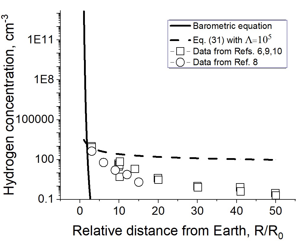
Figure 2: The hydrogen density vs. $R/R_{0}$ from the barometric equation, Eq. (31), and data from [8, 6, 9, 10].

The observed behavior of Terrestrial Exospheric profiles at several Earth radii ($R_{E}$) from the Earth center [8, 6, 9, 10] can be compared with the predictions of Eq. (31). The existing geocoronal data derive the hydrogen concentration $n$, [8, 6, 9, 10] from optical measurements of the Lyman hydrogen emission assuming that the underlying Lyman excitations are due to Sun light.

Incorporating the renormalization of Eq. (29) does not change the equations (21) and (22), so the momentum flux ${\cal P}=mnv_{g}^{2}$ remains coordinate independent. However, Eq. (23) acquires a renormalizing factor $R_{0}/R$ originating from the additional multiplier of $v_{g}$. For example, the energy flux into the Sun’s atmosphere carried by the accreting hydrogen can be estimated as

$$w=\frac{mg_{S}}{4\sigma}\sqrt{\frac{g_{S}L_{S}}{2}}\frac{R_{0}}{R}.$$ (33)

Here, any quantity with a subindex $S$ indicates a parameter of the Sun. Using the gravity law, it is straightforward to see that $g_{S}\approx 30\times g$ and $L_{S}\sim L$. Therefore the Sun related energy flux is about 100 times higher than that of Earth, $w_{\rm Sun}\sim 10$ $\mu$W at its surface.

Our interpretation here relates the geocorona radiation to the gravitational energy of the falling hydrogen transferred to the atmosphere in the range of heights around $z_{c}$ (see Table 1) where interatomic collisions dominate. As estimated in Eq. (23), the power so released, $w\sim 0.1$ $\mu$W/cm² turns out to be two-tree orders of magnitude higher than the measured. [8, 12] That discrepancy can be attributed to the average kinetic energy of a falling hydrogen atom (estimated as $\langle mv_{g}^{2}\rangle\sim{\cal P}/n_{c}\sim 0.1$ eV) being insufficient to excite the Lyman series, so only rare atoms with energies much higher than the average can contribute to the geocorona glow. The same energy argument can possibly explain how the distribution of light emitting hydrogen in Fig. 2) can have a somewhat different coordinate dependence compared to the total hydrogen concentration.

Extending the above theory to the case of Sun’s corona, results in the prediction $w\sim 1-10$ $\mu$Wcm^-2, in fair agreement with the data. [13, 14, 15] We attribute this better agreement to the fact that the solar acceleration due to gravity is about 30 times greater than that of Earth. Therefore the characteristic energy of a fallen hydrogen atom may be sufficient to excite the Lyman series for the case of Sun.

V Caveats and other possible applications

An implicit simplification in our treatment is that the temperature is determined externally. This assumption ignores the heat produced by the release of gravitational potential energy of a falling gas even though its related energy flux was estimated in the above as $w\sim 0.1$ $\mu$W for Earth and $w\sim 10$ $\mu$W for Sun. Conceptually one could include the effects of this heating by noting that in a steady state solution the heat gain due to a condensing gas must be equal to the heat loss from the gas due to thermal conductivity and radiation. That formidable problem remains to be addressed.

Some insight can be obtained by noting that the increase in temperature caused by the accreting H₂ will be small close to the surface ($z\ll z_{c}$) because the incoming energy must be distributed to all the particles in the dense region. Also the heat flux at large distances ($z\gg z_{c}$) where $g\rightarrow 0$ will also lead to negligible heating. The conclusion is that there will be a region of max temperature at some altitude $z\sim z_{c}$. Although very qualitative, one can wonder if this hot zone might explain the existence of celestial coronas.

Another consequence of the instability we have found is that all celestial bodies are in a state of accreting hydrogen. This provides an explanation why the gas giants have grown to their present size and will continue to grow until they reach a critical mass needed for nuclear ignition. This conclusion contradicts the usual belief that celestial bodies are all in the process of loosing their hydrogen atmospheres.

The concept of hydrogen accretion is also consistent with the repetitive NOVA explosions, such as a NOVA T Coronae Borealis to explode once in about 80 years.[16, 17]

VI Conclusions

In summary, we have demonstrated the following:
1. The famous barometric equation has a finite range of applicability limited to the altitudes where the mean free path of molecules $l$ becomes comparable to the characteristic dimension $L$ determining the barometric predicted atmosphere decay.
2. In the complementary region, the atmosphere distribution is better described by the dilute gas laws, and its density exhibits power decay or even logarithmic decay vs. distance.
3. The atmosphere distribution exhibits an instability corresponding to H2 accretion where it flows from far away to all stellar objects.
4. The accretion corresponds to a certain momentum flux and energy flux ($w\sim 0.1$ $\mu$W for Earth and $w\sim 10$ $\mu$W for Sun) that may contribute to celestial coronas.
5. Other possible correlations include the observed long tails in the Earth atmosphere, the existence of gas giants that have grown to their present size, and repetitive NOVA explosions.

To avoid any misunderstanding, the process of hydrogen accretion by celestial bodies predicted here does not rule out the known competing processes of hydrogen evaporation. The two trends must be carefully compared for each set of parameters and correlated with observations.

References

- [1] M. Grimsditch, Could Unstable Atmospheres Explain the Sun’s Corona?, Unpublished (2020)
- [2] D. A. McQuarrie, Statistical Mechanics, Harper & Row Publishers, New York, London (1976).
- [3] Yu. L. Klimontovich, Statistical Theory of Open Systems, Springer 1995;
- [4] Byung Chan Eu, Kinetic Theory of Nonequilibrium Ensembles, Irreversible Thermodynamics, and Generalized Hydrodynamics, Springer 2016.
- [5] H. Struchtrup, Macroscopic Transport Equations for Rarefied Gas Flows. Approximation Methods in Kinetic Theory, Springer 2005.
- [6] Baliukin, I., Bertaux, J.-L.,Quemerais, E., Izmodenov, V., Schmidt, W. (2019). SWAN/SOHO Lyman alpha mapping: The hydrogen geocorona extends well beyond the Moon. Journal of Geophysical Research: Space Physics, 124, 861–885. https://doi.org/10.1029/2018JA026136
- [7] D. N. Ruzic and S. A. Cohen, Total scattering cross sections and interatomic potentials for neutral hydrogen and helium on some noble gases, J. Chem. Phys. 83, 5527 (1985); doi: 10.1063/1.449674
- [8] L. Wallace, C. A Barth, J. B. Pearce, K. K. Kelly, D. E. Anderson, Jr, W. G. Fastie, Mariner 5 masurement of the Earth’s Lyman alpha emission, J. Geophys. Res.75 3769-77(1970).
- [9] Cucho-Padin, G., Kameda, S., Sibeck, D. G. (2022). The Earth’s outer exospheric density distributions derived from PROCYON/LAICA UV observations. Journal of Geophysical Research: Space Physics, 127, e2021JA030211. https://doi. org/10.1029/2021JA030211
- [10] J. H. Zoennchen, H. K. Connor, J. Jung, U. Nass, and H. J. Fahr, Terrestrial exospheric dayside H-density profile at 3–15RE from UVIS/HDAC and TWINS Lyman-K data combine, Ann. Geophys., 40, 271–279, 2022 https://doi.org/10.5194/angeo-40-271-2022
- [11] T. Sakurai, Heating mechanisms of the solar corona, Proc. Jpn. Acad., Ser. B 93 (2017)
- [12] I. S. Shklovsky, On hydrogen emission in the night glow, Planet. Space Sci. Pergamon Press 1959. 1, 63 (1959)
- [13] Ch. Leinert, S. Bowyer, L.K. Haikala, M.S. Hanner, M.G. Hauser, A.-Ch. Levasseur-Regourd, I. Mann, K. Mattila, W.T. Reach, W. Schlosser, H.J. Staude, G.N. Toller, J.L. Weiland, J.L. Weinberg, A.N. Witt, The 1997 reference of diffuse night sky brightness, A&A Supplement series, 127, 1-99, January I (1998),
- [14] H. Kimura and I. Mann, Brightness of the solar F-corona, Earth Planets Space, 50, 493–499, (1998)
- [15] T. Pinter, L. Klocok, M. Minarovjech, M. Rybanský, M. The total brightness of the solar corona during the eclipse June 21st 2001, in Solar Variability as an Input to the Earth’s Environment, ESA Special Publication, vol. 535, p.243 (2003).
-
[16]
R. G. Andrews, New York Times, The Night Sky Will Soon Get ‘a New Star.’ Here’s How to See It.
https://www.nytimes.com/article/nova-new-star-t-coronae-borealis.html -
[17]
L. Perkins, NASA Blog, View Nova Explosion, ‘New’ Star in Northern Crown
https://blogs.nasa.gov/Watch_the_Skies/2024/02/27/view-nova-explosion-new-star-in-northern-crown/