Testing trajectory-based determinism via time probability distributions
Abstract
It is notorious that quantum mechanics (QM) cannot predict well-defined values for all physical quantities. Less well-known, however, is the fact that QM is unable to furnish probabilistic predictions even in emblematic scenarios such as the double-slit experiment. In contrast, equipped with postulate trajectories, Bohmian mechanics (BM) has inherited more predictive power. It follows that, contrary to common belief, QM and BM are not just different interpretations but distinct theories. This work formalizes the aforementioned assertions and illustrates them through three case studies: (i) free particle, (ii) free fall under a uniform gravitational field, and (iii) the double-slit experiment. Specifically, we introduce a prescription for constructing a flight-time probability distribution within generic trajectory-equipped theories. We then apply our formalism to BM and derive probability distributions that are unreachable by QM. Our results can, in principle, be tested against real experiments, thereby assessing the validity of Bohmian trajectories.
I Introduction
There are numerous physical and philosophical discussions related to quantum mechanics (QM). However, one fact remains undeniable: the quantum formalism has consistently succeeded in describing the distribution of detector clicks in experiments. This success might lead some to believe that it provides objective answers (though not interpretative) for all observable phenomena. However, a critical examination of some traditional experiments reveals that this is not always true. For example, consider a double-slit experiment [1, 2, 3, 4, 5, 6, 7], where the position of a particle is measured on a detection screen located at , with the sub-index “d” referring to the detector. Typically, the particle’s flight-time is neither controlled nor measured in such experiments. After many runs of the experiment, the observer constructs the experimental time-independent probability density , which describes the possible locations reachable by the particle, conditioned on the detection line . Now, how can one apply Born’s rule from the theoretical to fit the experimental data?
A first move towards answering this question consists of recognizing that is not a joint probability distribution for , , and . Instead, it refers to the probability density of finding the system at the location given that time is guaranteed to be . In this case, the notation 111To shorten the notation, whenever the sub-index of the symbol representing the probability density function repeats in its argument, we may omit the latter. For example, would be simply ., emphasizing the conditioning on , is preferred [8, 9, 10, 11, 12]. Rather than just allegorical rephrasing, this serves to stress that the distribution has to be built for a single well-defined value of time. Next, we can condition on :
| (1) |
Unless one post-selects the experimental data to a particular value of , which actually is never done in practice, we still do not have a formal comparison with . Of course, our first impulse would be to assign some mean value for time in Eq. (1) or even to integrate over some time window, but these would be extra assumptions. This underscores that experimental results cannot always be straightforwardly confronted with QM’s predictions.
Experiments like the ones quoted above are usually carried out in the far-field regime, so semiclassical analysis generally applies [13, 14, 15, 16]. Nevertheless, recent advancements in ultra-fast detector technology [17, 18, 19, 20] have made it possible to explore regimes where semiclassics is insufficient to describe the system’s behavior [13, 21]. Therefore, it is mandatory to develop a strategy to deal with time. A viable route to this end would be to search for a probability distribution for the flight-time, , and then use probability theory to obtain the desired distribution,
| (2) |
It turns out, however, that the formalism of QM does not provide any prescription for the construction of , thus remaining silent regarding the time distribution of clicks along the detection line .
As a first contribution of this article, we demonstrate that trajectory-equipped theories can naturally address this issue. After presenting a general argument, our attention will be directed towards Bohmian mechanics (BM) [22, 23], a model that reinstates determinism while upholding probabilistic predictions consistent with QM. Although different from ours, approaches are already known that use Bohmian trajectories to construct time probability distributions [24, 25, 26]. In fact, several trajectory-based models exist [27, 28, 29] that allow access to the probability distribution of time [30, 31, 32]. Other approaches to time in QM are worth citing. While the Kijowski method [33, 34] employs semiclassical approximations to derive temporal predictions, the Page-Wooters mechanism [35] considers time as an inaccessible coordinate that arises from correlations between subsystems of the global state. Similar approaches conceiving time as an emergent property of physical systems can be found in Refs. [36, 37, 38]. The spacetime-symmetric extension of QM [9] treats time on par with space, resulting in a Schrödinger equation for time. This approach has found application to the problem of the tunneling time [39]. Finally, there are phenomenological modeling approximations of the detection process that yield probability distributions of time, such as the absorbing boundary rule [40, 41, 42, 43], path-integral with absorbing boundary [44, 45, 46], and others [47, 48, 49, 50, 51]. Each of these approximations and formalisms can be tested using equation (2) as they access the probability distributions and , with the sole requirement being experimental data for comparison, without the need for experiments involving direct time measurements.
In this work, a formalism based on the hypothesis of trajectory-based determinism will be developed to derive spatial and temporal probability distributions. Supplemented with minimal assumptions, this formalism enables the computation of probability distributions and , and finally the one in Eq. (2). We then employ BM to give a concrete example of the formalism usage and compare our results with those of other approaches [24, 25, 52, 53]. Besides this introduction, the text is organized as follows. In Sec. II, we introduce the basis for our model, which involves two postulates and the development of conditional probability distributions, one of them for the flight-time. In Sec. III, we apply our formalism to some emblematic physical problems and compare our results with other approaches (when available). We close the article in Sec. IV with our final remarks.
II Trajectory-equipped theory (TET)
In this section, we present our formalism, treating separately two types of deterministic trajectories, namely, those defined in terms of a velocity field and those in phase space. To simplify the discussion, we restrict ourselves to the one-dimensional case.
II.1 Trajectories associated with a velocity field
In this scenario, trajectories emerge from a first-order differential equation , where is some real function representing the velocity field. Setting , the coordinate of the particle at , the coordinate of the particle at the instant is uniquely defined. As is the case in BM, is the only boundary condition needed, and the mechanical momentum of a particle of mass is just given by . Now, as far as the triple is concerned, here is the catch: just as the specification of and implies , the specification of and (respectively, and ) should imply (respectively, ). In addition, due to the functional structure connecting the triple, one variable inherits the uncertainties of the others, provided physical principles are not violated. We rigorously formalize these ideas as follows:
-
•
Determinism hypothesis.—There exists a smooth trajectory connecting an initial coordinate to a point over a time lapse . For bounded dynamics, is expected to be a recurrence point, reachable at several instants . Additionally, in typical well-behaved dynamics, is invertible (at least in parts). Therefore, there must be functions and allowing us to express determinism in terms of the relations
(3) with . In this trajectory-equipped theory (TET), probability distributions are given by
(4a) (4b) where denotes the Dirac delta function. As expected, here we have non-negative distributions satisfying .
-
•
Preparation independence hypothesis.— The probability distribution for derives from some experimental procedure that is in no way physically conditioned to and , hence
(5) The preparation should be specified in each statistical theory. In QM, , with the density operator at .
In what follows, we will build upon the previously mentioned assumptions, using the definition of marginal probability,
| (6) |
along with the property of the Dirac delta function,
| (7) |
where and for . Plugging the distributions (4a) and (5) into Eq. (6), and solving the integral over with the property (7), we obtain
| (8) |
The modulus operation appearing in the denominator guarantees that . The probability distribution for flight-times is constructed similarly. Using the relations (4b)-(7), we end up with
| (9) |
where the function is achieved from manipulating the equation so that .
For future reference, we now indicate how the probability distributions of flight-times and positions can be associated with each other, in particular in the BM context. Starting with , we can use the property (7) to write
| (10) |
where we have introduced . Multiplying Eq. (10) by and integrating over gives
| (11) |
In the specific case where , independently of , we find, from Eq. (9),
| (12) |
Specializing to BM, is readily identified with the velocity field, and with the absolute value of the probability current density, so we have
| (13) |
This formula is a generalization of the typical one [24, 25], valid only when is not a recurrence point . In fact, it is crucial to realize that our approach generalizes the existing one in two aspects. First, it applies to all trajectory-equipped theories, not only to BM. Second, it naturally accommodates bounded oscillatory dynamics, an issue that, to our knowledge, has remained unaddressed so far.
II.2 Phase space trajectories
We now consider trajectories defined in the phase space through real functions and , constrained by the initial condition at . Importantly, since and are treated as independent canonical variables, the uncertainties associated with and can similarly be independent. The initial probability distribution is denoted as or, equivalently, . For simplicity, in what follows, we assume that there are no recurrences (i.e., the trajectory passes through the point only once), so the inversion of the trajectories yields only the functions and . Again, we propose an approach relying on two fundamental assumptions.
-
•
Determinism hypothesis.—There exists a trajectory in phase space defined by smooth functions and , connecting an initial point to a final point over a time lapse . Assuming that the involved functions are invertible and that there are no recurring points, the determinism hypothesis can be expressed by the relations
(16) and
(19) Note that the symbol (respectively, ) refers to a function originating from the inversion of , with output (respectively, ). Similar reasoning has motivated us to name the other functions appearing in Eqs. (16) and (19). In addition, note that the pairs , , and consist of distinct functions. Based on these relations, we propose the following conditional probabilities:
(20a) (20b) (20c) The approach is such that starting with two postulated functions and involving the variables , one can construct a joint probability distribution for two of them out of the specification of the others. Note that while the distribution (20a) admits the interpretation , meaning that and are uncorrelated variables both conditioned to , the same does not hold for the ones involving time. Equation (20b), for instance, can be interpreted as , with the probability for one of the variables, , depending explicitly on the other. All this is consistent with the premise that and are independent canonical variables, while and are not.
-
•
Preparation independence hypothesis.—The joint probability for derives from some experimental procedure that is in no way physically conditioned to and , hence
(21) The preparation should be specified in each statistical theory. In QM, one possibility is to use the Husimi distribution [54], , where denotes a coherent state with complex label parametrized in terms of phase-space coordinates.
Utilizing the same procedure as before, we integrate the product of distributions (20a) and (21) over to obtain, with the aid of property (7),
| (22) |
where
| (23) |
and is found by isolating in the equation . Via similar procedures, from Eq. (20b), we obtain
| (24) |
where
| (25) |
and is found by isolating in the equation , and, from Eq. (20c),
| (26) |
where function is same one that appears in Eq. (22) and
| (27) |
III Case studies
In this section, we apply our formalism to simple physical systems and, when pertinent, we compare our results with those of other approaches.
III.1 Free particle
We start considering the one-dimensional dynamics of a free particle with mass , prepared in a Gaussian state written as , where
| (28) |
The parameter () is the mean position (momentum) and is the spatial uncertainty. For the role of TET, we choose two participants: classical statistical mechanics (or Liouvillian mechanics) and BM. For the classical model, the phase-space trajectory is given by
while stands for the phase-space initial distribution. The joint probability distribution is then obtained using equation (22). The result reads
where and “” stands for “classical”. Marginalizing over gives
| (29) |
where
| (30) |
As expected, these results plainly match the ones obtained from the Liouvillian formalism, where emerges from the application of the inverse map of the trajectory to the initial probability distribution [55]. In addition, , meaning that the classical distribution mirrors the quantum one, as already known for the free particle system.
To compute the flight-time probability distribution, we start from Eq. (26) to obtain
| (31) |
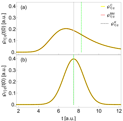
Now, to get , one needs to integrate this result over . Due to its complexity, the analytical result will be omitted, but it is numerically illustrated in Fig. 1, constrained to the detection position . This graph will be discussed later when confronted with the next approaches.
As a second TET, we consider BM. According to Bohmian theory, the trajectory for the free particle is given by [24]
| (32) |
With this function and its inverse , we come to Eq. (8) to show that . Through Eq. (9), we derive the flight-time distribution:
| (33) |
where the term inside the modulus is the velocity field .
We also bring to the discussion the distribution deriving from the Kijowski method [33, 34], which relies on the hypothesis of a generalized measurement operator for flight-time. Specifically for the arrival location and Gaussian state, the resulting distribution reads [34]
where is the step function.
In Fig. 1, we depict the distributions , , and for two sets of parameters. The first remark is that all theories yield precisely the same distribution. To a certain extent, this is not surprising, as the model under inspection is the simplest possible: the dynamics is linear, and the preparation is Gaussian. On the other hand, there is subtler information coming from the results. In the two panels considered, the mean velocities are identical, suggesting that the mean flight-times should be equal as well. However, this expectation is not confirmed due to the disparity in the masses. In panel (a), the mass is significantly smaller than the mass in panel (b), resulting in a larger spreading factor and, as a consequence, an enhancement of the temporal asymmetry induced the term . This effect can be clearly appreciated in the BM formalism through the relations (32) and (33). As illustrated in panel (b), the asymmetry in the time-probability distribution disappears as .
III.2 Free fall under a uniform gravitational field
Let’s delve into a scenario involving a freely falling particle, where the trajectory intersects the vertical coordinate at two distinct instances. As discussed previously, the TET posits that the probability distribution for flight-times is governed by Eq. (9) or, upon marginalization over , Eq. (26). In the present subsection, however, our study will be restricted to trajectories generated by a velocity field, implying that the latter equation does not apply. In addition, we will set TET to be BM. With this choice, we remind that the Muga-Leavens (ML) result is retrieved [24], with the caveat that it falls short in describing some systems involving recurrences (the back-flow problem). Here, the idea is to show that our formalism performs better than ML’s in characterizing the flight-time probability distribution when this behavior manifests. Given our purposes, the analysis of the free fall motion will be effectively restricted to one dimension, where we can directly apply our formalism.
Consider a particle of mass immersed in a uniform gravitational field and prepared in a Gaussian state expressed by , where () is the mean position (momentum) and is the initial spatial uncertainty. The Bohmian trajectory for this case is directly calculated as
| (34) |
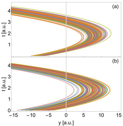
where is given in Eq. (30) and is the gravitational constant. In what follows, the parameters will be chosen to ensure that the particle crosses the coordinate at two distinct instants for practically all significant initial conditions . To illustrate this kind of dynamics, in Fig. 2, an ensemble of Bohmian trajectories (34) is showcased for two distinct sets of parameters. The choice of for each trajectory was taken considering the initial distribution , namely, the density of points is proportional to . As demanded, all trajectories shown in the graph have two passages through .
The flight-time probability distribution for the ML formalism derives from the probability current density [25]. Direct calculations yield
| (35) |
where the velocity field takes the form
| (36) |
is a normalization constant, and is the solution to the Schrödinger equation.
To apply our method (9), we first need to invert the function (34) to find solutions , for , corresponding to the two instants at which the trajectory crosses (see Fig. 2). This entails solving a quartic equation for time and then discarding two nonphysical roots. To discern the physical solutions, we require that , for any , and the consistency condition . Put simply, utilizing the inversion of the initial position , which is unique given and , allows for finding . If this initial condition is applied to the function and yields , the solution is deemed physical for a given time instant . This methodology aids in identifying the physical solutions for each time interval. Although these criteria suffice for finding the physical solutions in the current scenario, in more intricate cases, additional criteria may be necessary. For practical purposes, numerical calculations will be conducted to obtain the inverse trajectories and their derivatives, implementing them in Eq. (9).
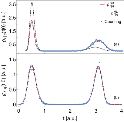
In Fig. 3, the flight-time probability distribution is depicted using the ML method (black dashed curve) and our formalism equipped with Bohmian trajectories (red solid curve). These results are also compared with a direct counting of the number of Bohmian trajectories (blue dots), according to the following procedure. We constructed an ensemble of initial positions, respecting the probability density of initial positions, . Then, we evolved each component of the ensemble using the Bohmian trajectory (34). Each time a trajectory intersected , we recorded its flight-time, and, at the end, we built the dotted distribution shown in Fig. 3. In panel (a), the agreement (disagreement) between our formalism (ML approach) and the direct counting is notable. This shows that the TET formalism is somewhat superior to the ML approach in describing systems exhibiting recurrences. The peaks of are located precisely over the most probable classical times, that is, the instants for which the center of the Gaussian distribution reaches . The distribution , on the other hand, fails to predict the second peak, the one for the recurrence time. As we approach a more classical regime (large mass), the velocity fields (36) at become more symmetric, in the sense that . In this regime, as discussed at the end of subsection II.1, the ML approach becomes as effective as ours [see panel (b)].
III.3 Double-slit experiment
Referring back to the problem discussed in the introduction, we now apply our formalism to provide a theoretical counterpart of for the double-slit experiment with particles, where the detection screen is situated in the line . The slits occupy the positions over the line . Here, we also use only BM as TET. Because the components and of the particle’s motion are decoupled from each other, we have at hand two independent one-dimensional problems, which are connected only by the variable time. For the direction, we take the usual wave-plane solution with box normalization:
| (37) |
where and are the component of the momentum and the energy of the system, respectively. Right after passing the slits, the component of the particle wave function reads
| (38) |
where . In the direction, the Bohmian trajectory is no different from the classical one: . Using the prescriptions (8) and (9), we obtain the distributions
| (39) |
and
| (40) |
where is the classical time taken by a particle of mass that crosses the slit and moves straight with momentum to reach the screen. Notice that, since the spatial distribution is uniform in the interval , the flight-time distribution is also uniform in the time interval . Thus, by substituting the formulas above into the prescription (2), we find
| (41) |
For added convenience, the integral will be carried out numerically.
In search of a counterpart to our result, we now supplement quantum mechanics (QM) with a (semi)classical element recognized as suitable in far-field regions. Specifically, we just substitute the classical time of flight, , in the prescription (1), in order to obtain , here denoted as
| (42) |
with “CT” standing for classical time. Such a result is expected to be appropriate solely for describing the far-field approximation scenario. As done previously, we construct a similar probability distribution by counting the number of Bohmian trajectories that cross the point from an ensemble of trajectories with initial conditions distributed according to . The result obtained from this direct counting is depicted in Fig. 4 with blue dots. The results obtained with our formalism, using BM as TET, are plotted as a solid black curve, while the quantum-mechanical approach supplemented with a classical time of flight is plotted as a solid red line.
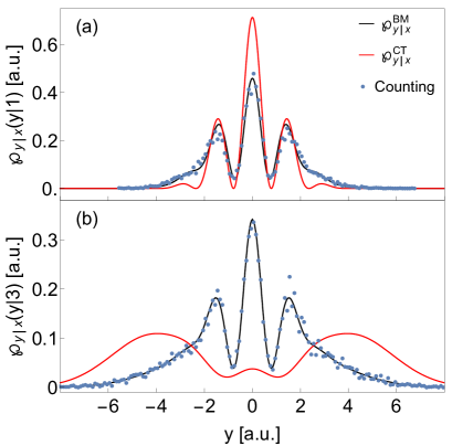
Although not always accentuated, the differences between the models and are perceptible and, in principle, measurable. In the near-field regime [panel (a)], where the two Gaussian branches of the wave function overlap significantly, both models predict the central interference pattern, but with different visibilities. In the far-field regime [panel (b)], the differences are remarkable and can be traced back to formulas (41) and (42). When we take to be large, and thus the flight-time , the latter formula allows the branches of the wave function to move far apart, reducing the overlap and preventing the central interference pattern from manifesting itself. On the other hand, formula (41) prescribes time averaging over several times, thus preserving the central interference pattern, albeit with low visibility. In other words, from an experimental standpoint, corresponds to statistically post-selecting for the specific time value . As for the counting result, it is noteworthy that it consistently corroborates our statistical formalism, which is based on .
As a final remark, we note that the lower visibility exhibited by in Fig. 4(a) might lead one to believe, when confronted with experimental data of this form, that the system is subjected to some source of decoherence. However, what is being shown here is that this effect derives solely from flight-time fluctuations; no spurious, uncontrollable degrees of freedom have been considered in our treatment. This raises an intriguing question about low-visibility experimental patterns. If one could guarantee the isolation of the system, then the low visibility could be seen as corroborating our theory.
IV Final remarks
In this work, we demonstrate that trajectory-equipped theories have a potential advantage over quantum mechanics in predicting the statistical outcomes of experiments involving flight-time fluctuations. Specifically, we show that by starting with the determinism hypothesis, a formalism can be developed [see Eqs. (8), (9), (22), (24), and (26)] that yields predictions for the flight-time probability distributions in emblematic experiments. From a theoretical viewpoint, this result is significant because it raises the perspective that Bohmian mechanics is not just an alternative interpretation of the standard quantum formalism, but rather provides predictions unreachable by the latter. More fundamentally, if confirmed empirically, these predictions will provide support for the idea of an underlying trajectory-based determinism spanning the quantum realm. On the other hand, if these predictions are not confirmed, then Bohmian mechanics would be ruled out. We hope that this work may stimulate researchers to test our results in the laboratory, which, we believe, is feasible with current technology.
V ACKNOWLEDGMENTS
This study was financed in part by the Coordenação de Aperfeiçoamento de Pessoal de Nível Superior - Brasil (CAPES) - Finance Code 001. R.M.A. and A.D.R. thank the financial support from the National Institute for Science and Technology of Quantum Information (CNPq, INCT-IQ 465469/2014-0). R.M.A. also thanks the Brazilian funding agency CNPq for Grant No. 305957/2023-6.
References
- [1] A. Zeilinger, R. Gähler, C. G. Shull, W. Treimer, and W. Mampe, Rev. Mod. Phys. 60, 1067 (1988).
- [2] R. Gähler, and A. Zeilinger, Am. J. Phys. 59, 316-324 (1991).
- [3] A. Tonomura, J. Endo, T. Matsuda, TT. Kawasaki, and H. Ezawa, Am. J. Phys. 57, 117-120 (1989).
- [4] R. Bach, D. Pope, S.-H. Liou, and H. Batelaan, New J. Phys. 15, 033018 (2013).
- [5] O. Carnal, and J. Mlynek, Phys. Rev. Lett. 66, 2689 (1991).
- [6] C. Kurtsiefer, T. Pfau, and J. Mlynek, Nature 386, 150-153 (1997).
- [7] C. Brand, S. Troyer, C. Knobloch, O. Cheshnovsky, and M. Arndt, Am. J. Phys. 89, 1132-1138 (2021).
- [8] L. Maccone, and K. Sacha, Phys. Rev. Lett. 124, 110402 (2020).
- [9] E. O. Dias, and F. Parisio, Phys. Rev. A 95, 032133 (2017).
- [10] D. R. Terno, Phys. Rev. A 89, 042111 (2014).
- [11] D. L. Sombillo, and E. A. Galapon, Ann. Phys. 364, 261-273 (2016).
- [12] A. A. Rafsanjani, M. Kazemi, A. Bahrampour, and M. Golshani, Commun. Phys. 6, 195 (2023).
- [13] N. Vona, G. Hinrichs, and D. Dürr, Phys. Rev. Lett. 111, 220404 (2013).
- [14] S. Das, M. Nöth, and D. Dürr, Phys. Rev. A 99, 052124 (2019).
- [15] D. Shucker, J. Funct. Anal. 38, 146-155 (1980).
- [16] S. Wolf, and H. Helm, Phys. Rev. A 62, 043408 (2000).
- [17] B. Korzh, et. al., Nat. Photonics 14, 250-255 (2020).
- [18] S. Steinhauer, S. Gyger, and V. Zwiller, Appl. Phys. Lett 118, 100501 (2021).
- [19] H. Azzouz, et. al., AIP Adv. 2, 032124 (2012).
- [20] M. Rosticher, et. al., Appl. Phys. Lett. 97, 183106 (2010).
- [21] F. Delgado, J. G. Muga, and G. García-Calderón, Phys. Rev. A 74, 062102 (2006).
- [22] D. Bohm, Phys. Rev. 85, 166 (1952).
- [23] D. Bohm, Phys. Rev. 85, 180 (1952).
- [24] C. R. Leavens, Phys. Rev. A 58, 840 (1998).
- [25] J. G. Muga, and C. R. Leavens, Phys. Rep. 338, 353-438 (2000).
- [26] S. Das, and D. Dürr, Scientific Rep. 9, 2242 (2019).
- [27] E. Nelson, Phys. Rev. 150, 1079 (1966).
- [28] M. J. W. Hall, D.-A. Deckert, and H. M. Wiseman, Phys. Rev. X 4, 041013 (2014).
- [29] F. McLafferty, The J. Chem. Phys. 83, 5043-5045 (1985).
- [30] H. Nitta, and T. Kudo, Phys. Rev. A 77, 014102 (2008).
- [31] M. J. Kazemi, and V. Hosseinzadeh, Phys. Rev. A 107, 012223 (2023).
- [32] A. Ayatollah Rafsanjani, M. J. Kazemi, V. Hosseinzadeh, and M. Golshani, Scientific Rep. 14, 3615, (2024).
- [33] J. Kijowski, Rep. Math. Phys. 6, 361-386 (1974).
- [34] I. L. Egusquiza, and J. G. Muga, Phys. Rev. A 61, 012104 (1999).
- [35] N. Page, and K. Wootters, Phys. Rev. D 27, 2885 (1983).
- [36] J. S. Briggs, and J. M. Rost, Eur. Phys. J. D 10, 311-318 (2000).
- [37] Eduardo O. Dias, Phys. Rev. A 103, 012219 (2021).
- [38] G. Sebastian, and J. M. Rost, Phys. Rev. Lett. 131, 140202 (2023).
- [39] R. Ximenes, F. Parisio, and E. O. Dias, Phys. Rev. A 98, 032105 (2018).
- [40] R. Werner, Ann. l’I.H.P. Phys. Théorique 47, 429-440 (1987).
- [41] R. Tumulka, Ann. Phys. 442, 168910 (2022).
- [42] R. Tumulka, Phys. Rev. A 106, 042220 (2022).
- [43] V. Dubey, C. Bernardin, and A. Dhar, Phys. Rev. A 103, 032221 (2021).
- [44] A. Marchewka, and Z. Schuss, Phys. Rev. A 63, 032108 (2001).
- [45] A. Marchewka, and Z. Schuss, Phys. Lett. A 240, 177-184 (1998).
- [46] A. Marchewka, and Z. Schuss, Phys. Rev. A 61, 052107 (2000).
- [47] T. Jurić, and H. Nikolić, Eur. Phys. J. Plus 137, 631 (2022).
- [48] S. Roncallo, K. Sacha, and L. Maccone, Quantum 7, 968 (2023).
- [49] J. A. Damborenea, I. L. Egusquiza, G. C. Hegerfeldt and J. C. Muga, Phys. Rev. A 66, 052104 (2022).
- [50] J. C. Muga, S. Brouard, and D. Macías, Ann. Phys. 240, 351-366 (1995).
- [51] J. J. Halliwell, Phys. Rev. A 240, 237-242 (1995).
- [52] A. J. Bracken, and G. F. Melloy, J. Phys. A: Math. Gen. 27, 2197 (1994).
- [53] H. Hofmann, Phys. Rev. A 96, 020101 (2017).
- [54] K. Husimi, Proc. Phys. Math. Soc. Jpn. 22, 264-314 (1940).
- [55] W. Greiner, Classical mechanics: Systems of particles and Hamiltonian dynamics (Springer-Verlag, Berlin, 2010).