Exploring field-evolution and dynamical-capture coalescing binary black holes in GWTC-3

Abstract

The continuously expanding sample of gravitational-wave observations is revealing the formation and evolutionary mechanism of merging compact binaries. Two primary channels, namely, isolated field binary evolution and dynamical capture, are widely accepted as potential producers of merging binary black holes (BBHs), which are distinguishable with the spin-orientation distributions of the BBHs. We investigate the two formation channels in GWTC-3, with a dedicated semi-parametric population model, i.e., a mixture of two sub-populations with different spin-orientation distributions (one is nearly-aligned and the other is nearly-isotropic). It turns out that the two sub-populations have different mass and mass-ratio distributions. The nearly-aligned sub-population, which is consistent with the isolated field formation channels, has a less preference for symmetric systems, and likely dominate the 10-solar-mass peak in the primary-mass function. While the isotropic sub-population shows a stronger preference for symmetric systems, and mainly contribute to the 35-solar-mass peak in the primary-mass function, consistent with the dynamical channels. Moreover, our results show that the purely isotropic-spin and the single well-aligned (i.e., the width of $\cos\theta$ distribution $\sigma_{\rm t}<0.5$) scenario are ruled out (by a Bayes factor of $\ln\mathcal{B}=5.2$ and $\ln\mathcal{B}=9.8$).

1 Introduction

Gravitational waves (GW) can bring us information about the coalescing compact binaries (Abbott et al., 2016), including, e.g., component masses, spin magnitudes, spin orientations, and luminosity distances of the sources, with which we can infer the formation/evolution of the coalescing compact binaries. Various formation channels have been proposed (e.g. Livio & Soker, 1988; Marchant et al., 2016; Mandel & de Mink, 2016; Fragione & Kocsis, 2018; Yang et al., 2019). Generally, formation channels fall into two categories: the isolated field binary evolutions and the dynamical formations (see Mapelli, 2018; Mandel & Farmer, 2022, and their refs.). With the rapidly increasing GW detections of compact binary coalescences (CBCs) (Abbott et al., 2019, 2021a; The LIGO Scientific Collaboration et al., 2021a, b), including binary neutron stars (BNSs) (Abbott et al., 2017, 2020a), binary black holes (BBHs) (Abbott et al., 2016), and neutron star-black holes (NSBHs) (Abbott et al., 2021b), one can reveal the formation/evolution channels of the CBCs in some statistical ways (e.g. Fishbach et al., 2020; Fishbach & Holz, 2020; Wang et al., 2021; Tang et al., 2021; Li et al., 2021a; Abbott et al., 2023), because the different formation scenarios will produce CBCs with different distributions of some physical parameters, such as mass, mass ratio, spin magnitude, and spin orientation. For instance, hierarchical mergers via dynamical formation channels are distinguishable (Gerosa & Fishbach, 2021), and recently we have identified the merger-origin BHs in the GWTC-3 (Li et al., 2023), because they have typical spin magnitudes ($\sim 0.7$) (Fishbach et al., 2017; Gerosa & Berti, 2017) and unusually high masses (lying in the pair-instability mass-gap (Woosley, 2017; Woosley & Heger, 2021)).

For the stellar-formed (or first-generation) BBHs, the spin-orientation distribution is one of the most significant features to tell their origins, whether the dynamical formation channels or the isolated field evolution channels. The BBHs from isolated field evolution will have spins nearly aligned with the orbital angular momentum (Rodriguez et al., 2016b; Gerosa et al., 2018); while the dynamically formed BBHs in the star clusters are expected to have isotropic spins (Stevenson et al., 2017; Farr et al., 2018). Though dynamical formation channel in the disks of active galactic nuclei may also produce BBHs with nearly aligned spins (Yang et al., 2019; Tagawa et al., 2021), this kind of mergers only take a negligible fraction in the stellar-formed BBHs (Li et al., 2023). Abbott et al. (2023) have investigated the spin-orientation ($\cos\theta_{1,2}$, i.e., cosine of the tilt angle between component spin and a binary’s orbital angular momentum) distribution of the BBHs using a parametric model $\pi(\cos\theta_{1,2}|\sigma_{\rm t},\zeta)=\zeta\mathcal{G}(\cos\theta_{1,2}|1,\sigma_{\rm t},-1,1)+(1-\zeta)\mathcal{U}(\cos\theta_{1,2}|-1,1)$, so called Default spin model. $\mathcal{U}(\cos\theta_{1,2}|-1,1)$ is a Uniform distribution in (-1,1) and $\mathcal{G}(\cos\theta_{1,2}|1,\sigma_{\rm t},-1,1)$ is a truncated Gaussian distribution in (-1,1), peaking at $\cos\theta_{1,2}=1$ (perfect alignment) with width of $\sigma_{\rm t}$. They find that either perfectly aligned spins ($\zeta=1~{}\&~{}\sigma_{\rm t}\sim 0$) or fully isotropic spins ($\zeta=0~{}||~{}\sigma_{\rm t}\gg 1$) is disfavored. However, in their analysis, the $\cos\theta_{1,2}$ distribution is independent from the mass function of the BBHs, which makes it hard to identify the nearly-aligned and isotropic-spin sub-populations. Therefore, in this work, we construct a population model aiming to identify sub-populations with different spin-orientation distributions, determining the mass and mass-ratio distributions of the sub-populations.

Comparing the BHs in different types of sources, may provides us with the information of formation / evolution processes about compact binaries. Fishbach & Kalogera (2022) compared the BHs in X-Ray binaries (XRBs) and GW sources, they found that the mass distributions of BHs in high-mass X-ray binaries (HMXB) and BBHs are consistent, when accounting for the GW observational selection effects; additionally, the BHs in low-mass X-ray binaries (LMXB) also have similar masses to BBHs with low-mass secondaries (i.e., $m_{2}<8M_{\odot}$). However, they found that the BHs in XRBs spin significantly faster than BBHs, so they suggested the BHs in the BBHs and XRBs are ‘Apple and Orange’. On the contrary, Belczynski et al. (2021) shows that the BHs in XRBs and BBHs may not form two distinct populations, so called ‘All Apples’. They suggest the real difference in mass between the two samples arises naturally from different formation environments, since metallicity regulates BH mass (Belczynski et al., 2010). Anyway, BBHs in the GWTC-3 (Abbott et al., 2019, 2021a; The LIGO Scientific Collaboration et al., 2021a, b) may be mixed of dynamically formed binaries and isolated field binaries (Livio & Soker, 1988; Marchant et al., 2016; Mandel & de Mink, 2016; Fragione & Kocsis, 2018; Yang et al., 2019; Li et al., 2022; Wang et al., 2022), and the dynamically formed binaries must have gone through different evolution processes from those of the XRBs. Therefore, it would be more effective to compare the BHs in XRBs with the BBHs from an individual channel, if the two types of formation channels are identified.

On the other hand, comparing the BHs mass functions of dynamically formed binaries and the mass function of underlying initial BHs (or the filed binary mass function), may also provide information about the formation environments of the dynamically formed binaries. For instance, O’Leary et al. (2016) found that dynamical interactions can enhance the merger rate of BBHs with total mass $M_{\rm tot}$ roughly as $\propto M_{\rm tot}^{\beta_{\rm M}}$ with $\beta_{\rm M}\gtrsim 4$, when including a background potential that mimics the underlying stellar cluster, however $\beta_{\rm M}\gg 4$ when this potential was absent. Additionally, dynamical formation is expected to produce more symmetrical BBHs than traditional field BBHs (i.e., common envelope channel) (see, e.g., Rodriguez et al., 2016a; Banerjee, 2017; Antonini et al., 2019; Zevin et al., 2021, and their references), which makes these two kinds of systems easier to classify.

In this work, we perform hierarchical Bayesian inference to explore the sub-populations of field-evolution and dynamical-capture binary black holes in GWTC-3. The work is organized as follows: In Section 2, we introduce the inference framework, data, and population models; in Section 3, we present the results; and in Section 4, we perform model comparisons and mock data studies to check the validation of the results. We make our conclusion and discussion in Section 5.

2 Methods

2.1 Framework and data

In this work, we perform hierarchical Bayesian inferences to infer the population properties of merging compact binaries from GW observations by LIGO/Virgo/KAGRA (Abbott et al., 2019, 2021a; The LIGO Scientific Collaboration et al., 2021a, b). We assume the distribution of merging compact binaries can be expressed by the population model $\pi(\boldsymbol{\theta_{i}}|\boldsymbol{\Lambda})$, where $\boldsymbol{\theta_{i}}$ are the parameters of the individual source including cosmological red-shift $z$, component masses $m_{1,2}$, spin magnitudes $a_{1,2}$, and cosine tilt angles that describe the spin orientations of two components $\cos\theta_{1,2}$; $\boldsymbol{\Lambda}$ are the hyperparameter, which describe the distribution of merging compact binaries. Following Abbott et al. (2021c) and Abbott et al. (2023), the likelihood of $\boldsymbol{\Lambda}$, given data $\{\boldsymbol{d}\}$ from $N_{\rm det}$ GW events, is expressed as

$$\mathcal{L}(\{\boldsymbol{d}\},N_{\rm det}|\boldsymbol{\Lambda},)\propto N^{N_{\rm det}}e^{-N{\xi(\boldsymbol{\Lambda})}}\prod_{i=1}^{N_{\rm det}}\int{\mathcal{L}(\boldsymbol{d_{i}}|\boldsymbol{\theta_{i}})\pi(\boldsymbol{\theta_{i}}|\boldsymbol{\Lambda})d\boldsymbol{\theta_{i}}},$$ (1)

where $N$ is the number of mergers in the Universe over the observation period, which is related to the merger rate. $\mathcal{L}(\boldsymbol{d_{i}}|\boldsymbol{\theta_{i}})$ is the single-event likelihood that can be estimated using the posterior samples (see Abbott et al. (2021c) for detail); $\xi(\boldsymbol{\Lambda})$ means the detection fraction, and it can be estimated using a Monte Carlo integral over detected injections as introduced in the Appendix of Abbott et al. (2021c). Since the Monte Carlo summations over samples to approximate the integrals will bring statistical error in the likelihood estimations Farr (2019); Talbot & Thrane (2020); Essick & Farr (2022); Golomb & Talbot (2022a, b); Talbot & Golomb (2023), we constrain the prior of hyperparameter to ensure $N_{{\rm eff},i}>10$, and $N_{\rm eff,sel}>4N_{\rm det}$, where $N_{{\rm eff},i}$ and $N_{\rm eff,sel}$ are the effective numbers of samples for $i$-th event and detected injections, respectively, as defined by Abbott et al. (2023); Farr (2019). In our analysis, we do not account for the spin-induced selection bias when calculating the observable fraction $\xi(\boldsymbol{\Lambda})$, this is because the injection samples are not enough for our model to estimate an accurate $\xi(\boldsymbol{\Lambda})$ . We find the conclusions in this work are not sensitive to the selection effects, because we have also performed an inference without selection effects, and the identification of the two sub-populations is unchanged.

As for the GW data, we use the ‘C01:Mixed’ posterior samples of BBHs in GWTC-3 (Abbott et al., 2019, 2021a; The LIGO Scientific Collaboration et al., 2021a, b), adopted from the Gravitational Wave Open Science Center. We use a size of 5000 for per-event samples instead of the minimum sample size across all events (i.e., 1993 of GW200129_065458), so that some narrow distributions may also pass the threshold of $N_{{\rm eff},i}>10$. Note that three events have sample sizes smaller than 5000 (i.e., GW150914_095045, GW200112_155838, and GW200129_065458 have sample sizes of 3337, 4323, and 1993, respectively), for these events, the posterior points are reused by random choice. This manipulation will not increase the effective numbers for these events, but will increase the effective numbers for the events which initially have more than 5000 samples given hyper-parameters $\boldsymbol{\Lambda}$ Following Abbott et al. (2023), we choose a false-alarm rate (FAR) of $1yr^{-1}$ as the threshold to select the events, and exclude GW190814 from our main analysis, since it is a significant outlier (Abbott et al., 2023; Essick et al., 2022) in the BBH populations. Consequently, 69 events are selected for our analysis. For all the hierarchical inferences, we use the Pymultinest (Buchner, 2016) sampler, to obtain the posterior distribution of the hyperparameter.

2.2 BBH population models

Previously, we found two subpopulations of coalescing BHs: one have a significantly larger spin-magnitude distribution (peaks at $\sim 0.7$), consistent with the higher-generation BHs in hierarchical mergers (Li et al., 2023); the other have a smaller spin-magnitude distribution and have an upper-mass cutoff (at $\sim 45M_{\odot}$) as expected by the pair-instability supernova (Woosley, 2017; Woosley & Heger, 2021)), which are consistent with the first-generation (or stellar-formed) BHs. In this work, we aim to find out the sub-populations of field-evolution and dynamical-capture binary black holes in the first-generation BBHs.

As was frequently studied, the dynamical formation channels predict an isotropic distribution for the spin orientations of the BHs (Mandel & Farmer, 2022), equivalently, $\cos\theta_{1,2}\sim\mathcal{U}(-1,1)$; On contrary, the isolated field binary BHs are likely to have spin orientations nearly aligned with the orbital angular momentum of the systems (Mandel & Farmer, 2022), where the distribution of $\cos\theta_{1,2}$ can be approximated as $\mathcal{G}(1,\sigma_{\rm ct},-1,1)$. Therefore, we take the $\cos\theta_{1,2}$ distributions as the key to distinguish the field and the dynamical formation channels for the first-generation BBHs. As for the component-mass functions of the first-generation BBHs for two formation channels, we apply the PowerLaw Spline model as first introduced by Edelman et al. (2022). It is a semi-parametric mass function relying on fewer assumptions, which makes it appropriate to find out the underlying mass distributions of BBHs from the two formation channels.

The mass and spin distributions of the field subpopulation can be expressed as

$$\pi_{\rm A}({\bf\theta})=P_{\rm m}(m_{1},m_{2}|{\bf\Lambda}_{\rm A})\times\mathcal{G}(\cos\theta_{1},\cos\theta_{2}|1,\sigma_{\rm t},-1,1)\times\mathcal{G}(a_{1},a_{2}|\mu_{\rm a,1},\sigma_{\rm a,1},0,1),$$ (2)

with

$$P_{\rm m}(m_{1},m_{2}|{\bf\Lambda}) =A({\bf\Lambda})\mathcal{PS}(m_{1}|\alpha,\delta,m_{\rm min},m_{\rm max};f(m|\{x_{i}\},\{f_{i}\}))$$ (3)

$$\times\mathcal{PS}(m_{2}|\alpha,\delta,m_{\rm min},m_{\rm max};f(m|\{x_{i}\},\{f_{i}\}))~{}(m_{2}/m_{1})^{\beta}~{}\Theta(m_{1}-m_{2}).$$

where $A({\bf\Lambda})$ is the normalization factor, $\Theta(m_{1}-m_{2})$ denotes the Heaviside step function ensuring $m_{1}>m_{2}$, and $\mathcal{PS}$ is the PowerLaw Spline model (Edelman et al., 2022). We use 10 knots $\{(x_{i},f_{i})\}_{i=1}^{10}$ to interpolate the perturbation function $f(m)$ of the mass distribution for first-generation BHs, and fix the locations of knots $\{x_{i}\}_{i=1}^{10}$ to be linear in the log space of (6, 60) $M_{\odot}$

In the absence of hierarchical mergers, we can similarly model the mass and spin distributions of the dynamical subpopulation as

$$\pi_{\rm I}({\bf\theta})=P_{\rm m}(m_{1},m_{2}|{\bf\Lambda}_{\rm I})\times\mathcal{U}(\cos\theta_{1},\cos\theta_{2}|-1,1)\times\mathcal{G}(a_{1},a_{2}|\mu_{\rm a,1},\sigma_{\rm a,1},0,1),$$ (4)

and then the mass and spin distribution of the first-generation BBHs can be expressed as

$$\pi({\bf\theta}|{\bf\Lambda})=[P_{\rm m}(m_{1},m_{2}|{\bf\Lambda}_{\rm A})\times \mathcal{G}(\cos\theta_{1},\cos\theta_{2}|1,\sigma_{\rm t},-1,1)\times(1-r_{\rm I})$$ (5)

$$+P_{\rm m}(m_{1},m_{2}|{\bf\Lambda}_{\rm I})\times \mathcal{U}(\cos\theta_{1},\cos\theta_{2}|-1,1)\times r_{\rm I}]\times\mathcal{G}(a_{1},a_{2}|\mu_{\rm a,1},\sigma_{\rm a,1},0,1),$$

here ‘A’ and ‘I’ denote the aligned and the isotropic subpopulations. This model can be considered as the extend/modified version of the Default spin model in Abbott et al. (2023) (firstly introduced by Talbot & Thrane, 2017), for we allow the aligned and the isotropic subpopulations to have respective mass functions. Here after in this work, Eq. 5 is named Extend Default.

However, in the presence of hierarchical mergers, when modeling the distribution of dynamical subpopulation, we should simultaneously consider the higher-generation BHs, which has significantly different spin-magnitude distribution ($\sim 0.7$) (Wang et al., 2022) and mass range ($\sim 20M_{\odot}-80M_{\odot}$)(Li et al., 2023). We assume the higher-generation BHs take a fraction of $r_{\rm 2G}$ in the dynamical subpopulation. Since the hierarchical mergers also have a fraction of nearly-aligned assembly (Li et al., 2023), as expected to be formed in gas-rich environments like AGN disks (Gerosa et al., 2015; Yang et al., 2019), we use $\mathcal{GU}(\cos\theta|\sigma_{\rm t,AGN},\zeta_{\rm AGN,2})=(1-\zeta_{\rm AGN,2})\times\mathcal{U}(\cos\theta|-1,1)+\zeta_{\rm AGN,2}\times\mathcal{G}(\cos\theta|1,\sigma_{\rm t,AGN},-1,1)$ to model the spin-orientation distribution of the higher-generation BHs, where $\zeta_{\rm AGN}$ is the fraction of the AGN-disk-originated BHs (in the higher-generation subpopulation), and $\sigma_{\rm t,AGN}$ is the width of $\cos\theta$ distribution of BHs in AGN disks. Meanwhile, we use $\mathcal{GU}(\cos\theta|\sigma_{\rm t,AGN},\zeta_{\rm AGN,1})$ to model the spin-orientation distribution of the first-generation dynamical BHs. Yang et al. (2019) find the proportion between the first-generation BHs and higher-generation BHs in AGN disks is $k\sim 3$ , then there is a relation $k~{}r_{\rm 2G}~{}\zeta_{\rm AGN,2}=(1-r_{\rm 2G})~{}\zeta_{\rm AGN,1}$, i.e., $\zeta_{\rm AGN,1}=k~{}r_{\rm 2G}\zeta_{\rm AGN,2}/(1-r_{\rm 2G})$. We constain $\zeta_{\rm AGN,1}<1$. Then the distribution of dynamically-formed BHs is expressed as

$$\pi_{\rm Dyn,BH}(m,a,\cos\theta |{\bf\Lambda}_{\rm Dyn,BH})=\mathcal{PS}(m|\alpha_{\rm D,1},\delta_{\rm D,1},m_{\rm min,D,1},m_{\rm max,D,1};f_{\rm D,1}(m|\{x_{i}\},\{f^{i}_{\rm D,1}\}))$$ (6)

$$\times \mathcal{G}(a|\mu_{\rm a,1},\sigma_{\rm a,1},0,1)\times\mathcal{GU}(\cos\theta|\sigma_{\rm t,AGN},\zeta_{\rm AGN,1})\times(1-r_{\rm 2G})]$$

$$+ [\mathcal{PS}_{\rm 2G}(m|\alpha_{\rm 2},\delta_{\rm 2},m_{\rm min,D,2},m_{\rm max,D,2};f_{\rm D,2}(m|\{x_{i}\},\{f^{i}_{\rm D,2}\}))$$

$$\times \mathcal{G}(a|\mu_{\rm a,2},\sigma_{\rm a,2},0,1)\times\mathcal{GU}(\cos\theta|\sigma_{\rm t,AGN},\zeta_{\rm AGN,2})\times r_{\rm 2G}.$$

Here we use another PowerLawSpline to model the mass function of higher-generation BHs, and for simplicity, we use 7 knots $\{(x_{i},f_{i,{\rm 2G}})\}_{i=1}^{7}$ to interpolate the perturbation function $f_{\rm 2}(m)$, and fix the locations of knots $\{x_{i}\}_{i=1}^{7}$ to be linear in the log space of (20, 80) $M_{\odot}$, as indicated by Li et al. (2023).

Then the mass and spin distribution of dynamical subpopulation can be expressed as

$$\pi_{\rm Dyn} (m_{1},m_{2},a_{1},a_{2},\cos\theta_{1},\cos\theta_{2}|{\bf\Lambda}_{\rm Dyn})=$$ (7)

$$B({\bf\Lambda}_{\rm Dyn})\times \pi_{\rm Dyn,BH}(m_{1},a_{1},\cos\theta_{1}|{\bf\Lambda}_{\rm Dyn,BH})\times\pi_{\rm Dyn,BH}(m_{2},a_{2},\cos\theta_{2}|{\bf\Lambda}_{\rm Dyn,BH})\times(m_{2}/m_{1})^{\beta_{\rm Dyn}}~{}\Theta(m_{1}-m_{2}).$$

where $B({\bf\Lambda}_{\rm Dyn})$ is the normalization factor. Therefore, in the presence of the hierarchical mergers, the total population is

$$\pi(\boldsymbol{\theta}|{\bf\Lambda})=\pi_{\rm Field}(\boldsymbol{\theta}|{\bf\Lambda}_{\rm Field})\times(1-r_{\rm D})+\pi_{\rm Dyn}(\boldsymbol{\theta}|{\bf\Lambda}_{\rm Dyn})\times r_{\rm D},$$ (8)

where $\pi_{\rm Field}(\boldsymbol{\theta}|{\bf\Lambda}_{\rm Field})$ is the distribution of the field BBHs as expressed as Eq. 2. Hereafter, the Eq. 8 is named Main Model in our work. We assume that the merger rate density increases with redshift, i.e., $\mathcal{R}(z)\propto(1+z)^{\gamma}$, and for simplicity, in all the models we fix $\gamma=2.7$ as reported in Abbott et al. (2023).

Table 1: hyperparameter and Priors for the analysis with full BBH catalog

descriptions	parameters	priors
		Field	Dynamical
			1G	2G
power-law slope of the primary mass distributions	$\alpha_{\rm F}/\alpha_{\rm D,1}/\alpha_{\rm D,2}$	U(-8,8)	U(-8,8)	U(-8,8)
smooth scale of the lower-mass edge	$\delta_{\rm F}/\delta_{\rm D,1}/\delta_{\rm D,2}[M_{\odot}]$	U(0,10)	U(0,10)	0
minimum mass cut off	$m_{{\rm min,F}}/m_{{\rm min,D,1}}/m_{{\rm min,D,2}}[M_{\odot}]$	U(2,10)	U(2,10)	U(20,50)
maximum mass cut off	$m_{{\rm max,F}}/m_{{\rm max,D,1}}/m_{{\rm max,D,2}}[M_{\odot}]$	U(20,100)	U(20,100)	U(60,100)
y-value of the spline interpolant knots	$\{f_{\rm F}^{j}\}_{j=2}^{9}/\{f_{\rm D,1}^{j}\}_{j=2}^{9}/\{f_{\rm D,2}^{j}\}_{j=2}^{7}$	$\mathcal{N}(0,1)$	$\mathcal{N}(0,1)$	$\mathcal{N}(0,1)$
power-law slope of the mass ratio distribution	$\beta_{\rm F}/\beta_{\rm D}$	U(-8,8)	U(-8,8)
width of the $\cos\theta_{1,2}$ distribution	$\sigma_{{\rm t,F}}/\sigma_{{\rm t,AGN}}$	U(0.1, 4)	U(0.1,1)
fraction of the dynamical sub-population (DynSubpop.)	$r_{\rm D}$	-	U(0,1)
fraction of the 2G BHs in DynSubpop.	$r_{\rm 2G}$	-	U(0,1)
fraction of the AGN-disk-originated BHs in 2G BHs	$\zeta_{\rm AGN,2}$	-	U(0,1)
ratio between 1G and 2G AGN-disk-originated BHs	$k$	-	3
constraint	$\zeta_{\rm AGN,1}\equiv k~{}r_{\rm 2G}\zeta_{\rm AGN,2}/(1-r_{\rm 2G})<1$
central value of spin-magnitude distribution	$\mu_{{\rm a,1}}/\mu_{{\rm a,2}}$	U(0,1)		U(0,1)
width of spin-magnitude distribution	$\sigma_{{\rm a,1}}/\sigma_{{\rm a,2}}$	U(0.05, 0.5)		U(0.05, 0.5)
local merger rate density	${\rm log}_{10}R_{0}[{\rm Gpc^{-3}yr^{-1}}]$	U(0,3)
power-law slope of the merger-rate evolution	$\gamma$	2.7

3 Results

With our Main Model, we again identify the higher-generation BHs with distinctive spin-magnitude distribution, which was first reported in our previous work (Li et al., 2023). See Appendix A, for the distribution of the first-generation and higher-generation BHs in the dynamical sub-population. Following, we mainly focus on the two sub-populations of field and dynamical formation channels for the first-generation BBHs.

3.1 Distributions of the field and the dynamical sub-populations

As shown in Figure 1, the Main Model finds out two sub-populations in the first-generation BBHs, which have significantly different mass and mass-ratio distributions. The $\sim 10M_{\odot}$-peak and the $\sim 35M_{\odot}$-peak in the primary-mass distribution, which are previously found by various approaches (Abbott et al., 2021c; Tiwari & Fairhurst, 2021; Li et al., 2021b; Edelman et al., 2022), may be dominated by the field and the dynamical channels, respectively. Interestingly, the mass distribution of the isotropic-spin sub-population in our results is nicely consistent with the mass distribution of BBHs in globular clusters by simulation (Antonini et al., 2023). Figure 4 displays the posterior distribution of the main parameters describing the two sub-populations; hereafter, all the values are for 90% credible level. The nearly-aligned sub-population takes a fraction of $12\%_{-6\%}^{+10\%}$ of the mergers, and the width of the $\cos\theta_{1,2}$ distribution is $\sigma_{\rm t}=0.74^{+0.58}_{-0.32}$, which is smaller/tighter than the result inferred by the Default model(Abbott et al., 2021c, 2023). The upper-mass cutoff of the field (the dynamical first-generation) sub-population is $m_{\rm max,F}=48.67^{+42.45}_{-22.68}M_{\odot}$ ($m_{\rm max,D,1}=38.38^{+12.60}_{-3.35}M_{\odot}$), which are consistent with the expectation of the (pulsational) pair-instability supernova ((P)PISN) explosions (Woosley, 2017; Woosley & Heger, 2021). Though the $m_{\rm max,F}$ is only loosely constrained (which is caused by the steep power-law slope of the mass function), the mass of the 99th percentile for the field sub-population is constrained to be $m_{99\%}=28.59^{+14.40}_{-6.79}M_{\odot}$ (see Figure 5). The spin-magnitude distribution peaks at $\mu_{\rm a}=0.11^{+0.06}_{-0.09}$ with standard deviation of $\sigma_{\rm a}=0.12^{+0.07}_{-0.05}$, which is consistent with the first-generation BHs inferred by the previous work (Li et al., 2023).

In particular, we infer $\alpha_{\rm D,1}<\alpha_{\rm F}$ at 98.5% credible level, as shown in Figure 2 (left), which indicates that the dynamical channels have a stronger preference to produce high-mass BBH mergers than the field channels, assuming the initial BH mass functions of two channels are similar. This may be because the BBHs formed by dynamical interactions in globular clusters, particularly three-body binary formation, will be enhanced by the total masses ($M_{\rm tot}$) of the binaries as $\propto M_{\rm tot}^{\beta_{\rm M}}$ with $\beta_{\rm M}\gtrsim 4$ (O’Leary et al., 2016). In the presence of hierarchical mergers, we do not find strong evidence for $\beta_{\rm D}>\beta_{\rm F}$, this may be because that the dynamical subpopulation contain ‘2G+1G’ systems (i.e., the hierarchical mergers with only one higher-generation BH) (Li et al., 2023). However when we inferring using the Extend Default model without hierarchical mergers, we find $\beta_{\rm I}>\beta_{\rm A}$ at 95.4% credible level, as shown in Figure 2 (the orange curves in the right panel). Such a result is consistent with the previous investigation of the mass-ratio distribution by an independent analysis (Li et al., 2022), i.e., there is divergence in mass-ratio distributions between low-mass and high-mass BBHs. Additionally, our results are also consistent with the prediction of the simulation studies (Rodriguez et al., 2016a; Banerjee, 2017).

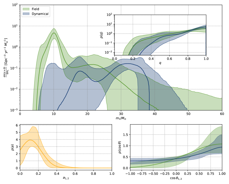
Figure 1: Reconstructed primary-mass, spin-magnitude, and cosine-tilt-angle distributions of the first-generation BBHs for each sub-population inferred with Main Model; the upper panel shows the differential local-universe merger rate as a function of primary mass. The solid curves are the mean values and the colored bands are the 90% credible intervals; the insets are for the mass-ratio distributions of the two sub-populations.

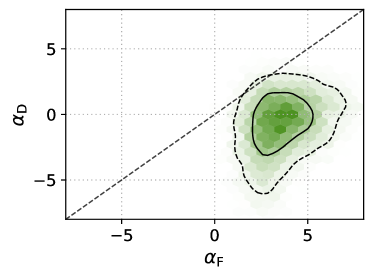
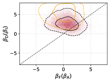
Figure 2: Posterior distributions of the power-law slopes of mass functions (left) and mass-ratio distribution (right) of the two sub-populations; the dashed and solid contours mark the central 50% and 90% posterior credible regions, respectively. The black curves are for the inference using the Main Model with hierarchical mergers; while the orange curves are for the inference using the Extend Default model without hierarchical mergers.

4 model comparison and results check

In this section, we firstly compare our model to some other alternative models with some specific assumptions; and then perform mock injection studies to check the validation of the results in section 3.

In our previous work (Li et al., 2023), other (single-population) models, such as the popular Default spin model (accompanied with the ‘PP’ or ‘PS’ mass model) (Abbott et al., 2023), are disfavored compared to the multi-population models that accounts for correlation between mass and spin-magnitude distributions of BHs (Li et al., 2023). In this work, we have found two different formation/evolution channels (i.e., field binary evolution and dynamical formation), which are expected to be distinguishable by the spin-orientation distributions of BBHs (Rodriguez et al., 2016b; Gerosa et al., 2018; Stevenson et al., 2017; Farr et al., 2018). Since most of other models do not include the main correlation between mass and spin-magnitude distributions (Li et al., 2023), it is appropriate to leave out the hierarchical mergers from our analysis when performing model comparison. This is because in the presence of higher-generation BHs (i.e. the high-spin BHs), the other models (e.g., the popular Default spin model) are disfavored compared to our main model, mostly due to their failure to fit the spin-magnitude distribution of higher-generation BHs found by our previous work (Li et al., 2023). This leave-out analysis may change the inferred mass functions of the two first-generation subpopualtions (i.e., the field and the dynamical), but will not affect the classification of them, i.e., the distribution tendency are not changed as shown in Figure 6.

In practice, GW170729_185629, GW190517_055101, GW190519_153544, GW190521_030229, GW190602_175927, GW190620_030421, GW190701_203306, GW190706_222641, GW190929_012149, GW190805_211137, GW191109_010717, and GW191230_180458 are leaved out, for they all have probabilities of $>0.5$ to be hierarchical mergers, according to Li et al. (2023). As is introduced in subsection 2.2, the Extend Default (i.e., Eq. 5) can model the field and the dynamical first-generation population, in the absence of hierarchical mergers. Therefore in this section, we adopt the Extend Default for model comparison and mock data studies. As shown in Figure 7 the inferred results of the leave-out analysis are similar to that inferred from the full catalog with Main Model (Eq. 8).

4.1 Model comparison

Table 2: Model comparison

Models	$\ln{\mathcal{B}}$
Extend Default	0
Default	-1.8
Single nearly-aligned	-1.2
Single isotropic-spin	-5.2
With two independent spin-magnitude distributions	-1.8
Extend Default ($\sigma_{\rm t}<0.5$)	1.5
Default ($\sigma_{\rm t}<0.5$)	-2.3
Single nearly-aligned ($\sigma_{\rm t}<0.5$)	-9.8

Note: these log Bayes factors are relative to the Extend Default model in our work.

For Bayesian model comparison, $\ln\mathcal{B}>2.3$ ($\ln\mathcal{B}>3.5$) is interpreted as a strong (very strong) preference for one model over another, and $\ln\mathcal{B}>4.6$ as decisive evidence (Jeffreys, 1961). We have also inferred using a model that only accounts for the single nearly-aligned or isotropic-spin population (See Appendix B.4 for details of the model). As shown in Table 2, the population of only isotropic-spin BBHs is disfavored, which means that merging BBHs are not solely dynamically formed in clusters. Though the single nearly-aligned model can not be easily ruled out, we infer the width of $\cos\theta$ distribution $\sigma_{\rm t}>0.7$ at 97% ($\sigma_{\rm t}>0.6$ at 99.9%) credible level, which is inconsistent with the isolated evolution of field binaries (Rodriguez et al., 2016b).

Since a large $\sigma_{\rm t}$ for the truncated Gaussian distribution allows a significant fraction of highly misaligned or anti-aligned BBHs, which is unlikely produced by the isolated field channels (Rodriguez et al., 2016b), we have also inferred with a restriction of $\sigma_{\rm t}<0.5$ in our models, see Appendix B.2 for more details. As shown in Table 2, with the restriction of $\sigma_{\rm t}<0.5$, our Extend Default is even more favored, however the other models are less favored.

One may also ask is it still possible that the nearly-aligned and isotropic-spin population follows the same mass function? i.e., the Default Spin model with a PowerLawSpline mass model. We find this model is slightly less favored than our Extend Default by a Bayes factor of $\ln\mathcal{B}=-1.8$. However this model is strongly disfavored by a Bayes factor of $\ln\mathcal{B}=-3.8$ comparing to the Extend Default, if we restrict $\sigma_{\rm t}<0.5$.

Additionally, we have also inferred using a model assuming that the spin magnitudes of the BBHs in two sub-populations follow two independent distributions (see Appendix B.6 for details), and found the spin-magnitude distributions of the two sub-populations are nearly identical as shown in Figure 13; what’s more, this model is slightly disfavored compared to our Extend Default. Therefore, with current GW data, there is no evidence that the spin magnitudes of first-generation merging BBHs are different between the field (nearly-aligned) and dynamical (isotropic-spin) sub-populations.

In the parameter estimation of individual GW events, the $\cos\theta_{1}$ is likely to be better measured than the $\cos\theta_{2}$ in the parameter (Abbott et al., 2019, 2021a; The LIGO Scientific Collaboration et al., 2021a, b). Therefore, we also perform an inference in absence of the $\cos\theta_{2}$, but our conclusion is unchanged, see Appendix B.5 for the results of the inference. Interestingly, the width of $\cos\theta_{1}$ distribution becomes smaller as $\sigma_{\rm t}=0.43^{+0.53}_{-0.26}$, such a result is expected by the binaries from the field evolution (Rodriguez et al., 2016b).

4.2 mock data studies

To test the validation of our results, we perform the injections, recovery, and hierarchical inferences of mock populations of BBH events. We respectively generate two kinds of mock populations: one (here after ‘Two pop’) has population properties the same as those we have inferred from the real data, and the other (here after ‘One pop’) does not have the feature of the spin-orientation distributions found in this work, see Appendix D for the details.

Then we use the Extend Default model to infer the underlying mock populations, respectively. We find similar features as we have found in the real data from the ‘Two pop’ mock population, i.e., there are two subpopulations with different mass, spin-orientation, and mass-ration distributions, as shown in Figure 14. We obtain the width of the $\cos\theta$ distribution of the aligned subpopulation as $\sigma_{\rm t}=0.6^{+0.23}_{-0.20}$, this value is similar to the results inferred from the real data, but larger than our injection of $\sigma_{\rm t}=0.3$. This indicates that the real $\cos\theta$ distribution for the aligned subpopulation of BBHs may be narrower than we inferred, and would be more consistent with the expectation about the isolated field binaries (Rodriguez et al., 2016b). For the ‘One pop’ mock population, we do not find two significant subpopulations with different mass distributions, as shown in Figure 15, because the spin-orientation distributions are all the same in all the mass range. These mock population studies support that the inferred features of BBH population from the real data are reliable, though we can not rule out that our analysis could be affected by other systematic biases, e.g., the biases in the waveform models used for parameter estimation.

5 conclusion and discussion

With the rapidly growing catalog of GW events, the formation and evolution histories of the coalescing compact binaries are being revealed by population analysis. Using the data of GWTC-3 (Abbott et al., 2019, 2021a; The LIGO Scientific Collaboration et al., 2021a, b), we explore the BBHs from two types of channels, i.e., field binary evolution and dynamical capture. Beside the population of hierarchical mergers identified by our previous work (Li et al., 2023), the first-generation BBHs can also be categorized into two sub-populations based on the spin-orientation, mass, and mass-ratio distributions. One sub-population with isotropic spins (i.e., consistent with the dynamical formation channels) have a stronger preference for symmetrical systems, and they may contribute to the $\sim 35M_{\odot}$-peak in the primary-mass function found in previous literatures (Abbott et al., 2021c). The other sub-population with nearly-aligned spins (i.e., expected by the isolated field evolution channels) contain more asymmetrical systems, which likely dominate the $\sim 10M_{\odot}$-peak in the primary mass distribution (Tiwari & Fairhurst, 2021; Li et al., 2021b; Edelman et al., 2022). The mass distribution of the isotropic-spin sub-population is flatter than that of the nearly-aligned-spin sub-population, which is consistent with the fact that dynamical formation channels will enhance the merger rate of heavier black hole binaries (O’Leary et al., 2016; Antonini et al., 2023).

Assuming the nearly-aligned and isotropic-spin sub-populations are exactly the field and dynamical BBHs, we compare the two sub-populations to the HMXB BHs, see Appendix E. The primary-mass distribution of the field BBHs may be lower than the mass distribution of BHs observed in HMXBs, while the mass distribution of the HMXB BHs may be consistent with the inferred initial mass function of the BHs in the environment for dynamical channels, which is the modified mass function of dynamical BBHs with $\alpha=\alpha_{\rm I}+2$ as indicated by O’Leary et al. (2016).

In this work, there is a key point for identifying the two sub-populations of field and dynamical channels: when identifying the field and dynamical BBHs based on their spin-orientation distributions, one should firstly model (or exclude) the hierarchical mergers, which contain BHs with significantly larger spin magnitudes ($\sim 0.7$) (Fishbach et al., 2017; Gerosa & Berti, 2017; Gerosa & Fishbach, 2021). Some parametric models (Kimball et al., 2021; Wang et al., 2022) have found the evidence for hierarchical mergers; what’s more, with a semi-parametric model, we have previously identified a sub-population of higher-generation BHs (Li et al., 2023), which is again found in this work (see Figure 3). If one (mis-) model all the BBHs with single spin-magnitude distribution, then the measurement of the spin-tilt distribution will be influenced (Miller et al., 2024). Additionally, a large per-event sample size (like 5000 posterior points per event as adopted in this work) is recommended for analysis. Because the potential sub-populations may have narrower spin-magnitude and the spin-orientation distributions than those of the total population, if the per-event samples are not sufficient, then the narrow distributions will be mistakenly ruled out (Talbot & Golomb, 2023).

Vitale et al. (2022) has analyzed the spin-tilt distribution of the BBHs with GWTC-3, and found no evidence for the $\cos\theta$ distribution peaking at $+1$. They modified the Default spin model with a variable $\mu_{\rm t}$ to fit the $\cos\theta$ distribution, and found $\mu_{\rm t}=0.48^{+0.46}_{-0.94}$ (the prior distribution is [-1,1]). We also perform inference with a variable $\mu_{\rm t}$ for the Extend model in this work, and find $\mu_{\rm t}=0.74^{+0.23}_{-0.38}$ as show in Figure 10. The mass and spin-magnitude distributions of the two subpopulations are unchanged, and the $\cos\theta$ distribution of the aligned subpopulation is only slightly shifted, as shown in Figure 9. Abbott et al. (2023) also find a flatter $\cos\theta$ distribution in GWTC-3 than in GWTC-2, while we find a narrower $\cos\theta$ distribution for the nearly aligned subpopulation, which may be partially attributed to the different modeling of spin-magnitude versus mass distribution. In this work, $\sigma_{\rm t}$ only describes the wide of $\cos\theta$-distribution for the first generation BBHs, not influenced by the higher-generation BHs. Additionally, the sizes of per-event samples may also cause the different $\cos\theta$ distributions between our result and that of Abbott et al. (2023) (see supplemental materials of Li et al. (2023) for more details), since a small sample size only allow flatter distributions given a threshold of $N_{{\rm eff},i}$.

Baibhav et al. (2023) has also analyzed the populations of BBHs with isotropic and aligned-spin orientations with GWTC-3, and found no evidence that the BHs from the isotropic-spin population possess different distributions of mass ratios, spin magnitudes, or redshifts from the preferentially aligned-spin population. Though they do not investigate the component-mass distribution depending on the spin alignment as we do, they do find that the dynamical and field channels cannot both have mass-ratio distributions that strongly favor equal masses. Indeed, in the results of Baibhav et al. (2023), the isotropic-spin population is more likely to favor equal-mass systems (see their Figure.1), which is consistent with our results. Callister et al. (2021) firstly found that the unequal-mass BBHs have larger effective spins with GWTC-2 (Abbott et al., 2019, 2021a), which was further confirmed by Abbott et al. (2023) using GWTC-3 (Abbott et al., 2019, 2021a; The LIGO Scientific Collaboration et al., 2021a, b). Our previous work (Li et al., 2023) indicates the hierarchical mergers may contribute to the anti-correlation between $q$-$\chi_{\rm eff}$ of BBHs. In this work, the field BBHs are also potentially contribute to the anti-correlation between $q$-$\chi_{\rm eff}$, because they have less preference for equal-mass system and have more preference for aligned spins.

With an astrophysical-motivated parameterization, Wang et al. (2022) show that the $\sim 10M_{\odot}$-peak and $\sim 35M_{\odot}$-peak in the primary-mass distribution are consistent with the field and dynamical BBHs. With a non-parametric population model Godfrey et al. (2023) has also found that the $\sim 10M_{\odot}$-peak in the primary-mass distribution is associated with isolated binary formation. However, contrary to our results, Godfrey et al. (2023) suggests the events at $\sim 35M_{\odot}$-peak have spins consistent with the $\sim 10M_{\odot}$ events. The difference (between our results and those of Godfrey et al. (2023)) may be caused by the fact that, the models in Godfrey et al. (2023) have only two subpopulations when fitting the data with hierarchical mergers. Thus the identification of the two subpopulations is dominated by the spin-magnitude distributions, since the hierarchical mergers contain BHs with spin magnitudes $\sim 0.7$ (Gerosa & Fishbach, 2021). The $\sim 35M_{\odot}$-peak BHs have low spin magnitudes different from the higher-generation BHs (Li et al., 2023), so Godfrey et al. (2023) find it consistent with the $\sim 10M_{\odot}$-peak BHs. We note in the results of Godfrey et al. (2023), the SpinPop_A of the Isolated Peak Model indeed have a preference for aligned spins. However, the SpinPop_A of the Peak+Continuum Model show less preference for alignment, caused by the contribution from $\sim 35M_{\odot}$-peak BHs (see Figure. 4 of Godfrey et al. (2023). This indicated the $\sim 35M_{\odot}$-peak BHs may be associated with the dynamical channels. Very recently, Ray et al. (2024) search for binary black hole sub-populations using binned Gaussian processes. The authors also find that the sub-population showing a feature at $\sim 30-40M_{\odot}$ is associated with dynamical formation in globular clusters, which is consistent with our results.

The dynamical evolution is expected to produce more mergers with equal mass components (Rodriguez et al., 2016a; Banerjee, 2017; Antonini et al., 2019; Zevin et al., 2021), because the comparable mass binaries have a higher binding energy to form tighter systems and merge within shorter durations. However, isolated field binaries via common envelopes may sometimes produce BBH mergers with unequal component masses, especially at lower metallicities (Spera et al., 2019; Mandel & Farmer, 2022). These predictions are clearly supported by our result, that the mass-ratio distribution of the dynamical-capture sub-population is steeper than that of the field-evolution sub-population at 99% credible level. Note that some scenarios of field evolution can produce more symmetric BBHs (Mandel & Farmer, 2022), like homogeneous chemical evolution (de Mink & Mandel, 2016; Marchant et al., 2016), and some dynamical channels may mildly prefer unequal mass components (Michaely & Perets, 2019), these channels, if exist, should not dominate the total population.

Spin-orientation distribution of the field BBHs may also be mass-dependent, because lighter BBHs are easier misaligned due to natal kicks (Rodriguez et al., 2016b), we are exploring such tendency in the future with more GW data (Abbott et al., 2018). The fourth observing run (O4) of the LIGO, Virgo, and KAGRA GW detectors have been going on, and the event samples are unprecedentedly rapidly increasing (see https://gracedb.ligo.org/latest/). More than twice as many events in O3 will be observed in O4 (Mandel & Farmer, 2022), and we will have $\gtrsim 200$ BBHs events in total, within one year; additionally, many other types of events may also be observed (Abbott et al., 2022; The LIGO Scientific Collaboration et al., 2022). In future work, we will optimize our method to incorporate more kinds of BHs and BBH formation channels (Cai et al., 2018; Franciolini et al., 2022; Cheng et al., 2023; Mandel & Farmer, 2022), which should provide more insights and stronger constraints on sub-population properties, with the increased GW samples.

Appendix A The higher-generation BHs

It has been widely discussed that the hierarchical mergers contain BHs with significantly spin-magnitude and component mass distributions (Fishbach et al., 2017; Gerosa & Berti, 2017; Gerosa & Fishbach, 2021). Evidence for hierarchical mergers was also found with some parametric methods (Kimball et al., 2021; Wang et al., 2022). Previously, we have identified the higher-generation BHs with a semi-parametric population model (Li et al., 2023). In this work, we aim to identify the field and dynamical formation channels for the first-generation BBHs based on the spin-tilt distributions. It is critical to properly model the mass and spin distributions of the higher-generation BHs, otherwise they will affect modeling of the spin distribution of first-generation BHs (Miller et al., 2024). With our Main Model, we again identify the higher-generation BHs in the dynamical subpopulation, which have significantly different spin-magnitude and mass distributions from the first-generation BHs, as shown in Figure 3. The higher-generation BHs take a fraction of $18^{+12}_{-9}\%$ in the dynamical channels, as shown in Figure 4.

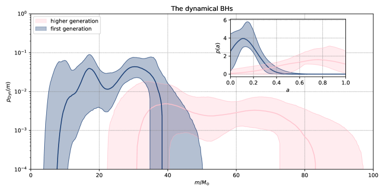
Figure 3: Reconstructed component-mass distributions of first-generation and higher-generation BHs in the dynamical subpopulation. The solid curves are the mean values and the colored bands are the 90% credible intervals; the insets are for the spin-magnitude distributions.

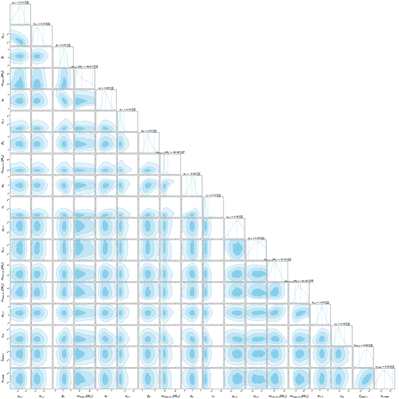
Figure 4: Posterior distribution of main parameters describing the full BBH population, inferred with the Main Model; the dashed lines in the marginal distribution represent the 90% credible intervals.

Figure 5: The mass of 99th percentile and the maximum mass of the field BBHs, inferred with the Main Model.

Appendix B Results of other models

B.1 Extend Default model

The priors for the Extend Default model are summarized in Table 3. Figure 6 shows the primary-mass, spin-magnitude, and cosine-tilt-angle distributions of the aligned-spin and isotropic-spin sub-populations of the first generation BBHs, inferred with the Extend Default model. And Figure 7 shows the posterior distributions of all the hyperparameters describing the two sub-populations.

Table 3: hyperparameter and Priors for the Extend Default

descriptions	parameters	priors
		nearly-aligned assembly	isotropic-spin assembly
power-law slope of the primary mass distributions	$\alpha_{\rm A}/\alpha_{\rm I}$	U(-4,12)	U(-4,4)
smooth scale of the lower-mass edge	$\delta_{\rm A}/\delta_{\rm I}[M_{\odot}]$	U(1,10)	U(1,10)
minimum mass cut off	$m_{{\rm min,A}}/m_{{\rm min,I}}[M_{\odot}]$	U(2,10)	U(2,10)
maximum mass cut off	$m_{{\rm max,A}}/m_{{\rm max,I}}[M_{\odot}]$	U(20,60)	U(20,60)
power-law slope of the mass ratio distribution	$\beta_{\rm A}/\beta_{\rm I}$	U(-4,8)	U(-4,8)
y-value of the spline interpolate knots	$\{f_{\rm A}^{j}\}_{j=2}^{9}/\{f_{\rm I}^{j}\}_{j=2}^{9}$	$\mathcal{N}(0,1)$	$\mathcal{N}(0,1)$
Width of the $\cos\theta_{1,2}$ distribution	$\sigma_{{\rm t}}$	U(0.1, 4)	-
mixing fraction of the isotropic-spin assembly	$r_{\rm I}$	-	U(0,1)
Central value of spin-magnitude distribution	$\mu_{{\rm a}}$	U(0,1)
Variance of spin-magnitude distribution	$\sigma_{{\rm a}}$	U(0.02, 0.5)
local merger rate density	${\rm log}_{10}R_{0}[{\rm Gpc^{-3}yr^{-1}}]$	U(0,3)
power-law slope of the merger-rate evolution	$\gamma$	2.7

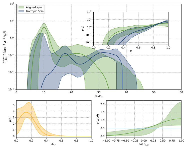
Figure 6: Reconstructed primary-mass, spin-magnitude, and cosine-tilt-angle distributions of BBHs for each population, inferred with the Extend Default model. The upper panel shows the differential local-universe merger rate as a function of primary mass. The solid curves are the mean values and the colored bands are the 90% credible intervals; the insets are for the mass-ratio distributions of the two sub-populations.

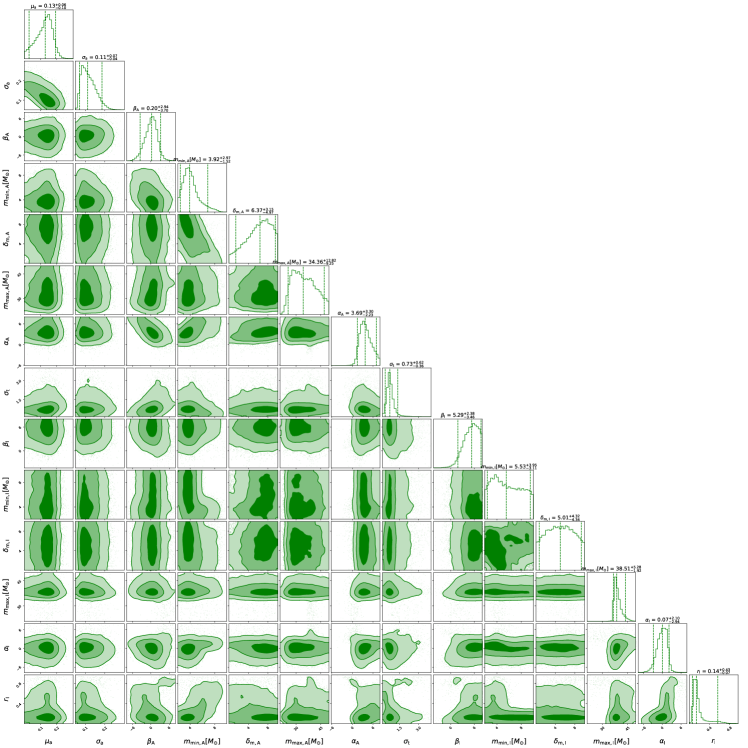
Figure 7: Posterior distributions of all the hyperparameters describing the two sub-populations, inferred with the Extend Default model; the dashed lines in the marginal distribution represent the 90% credible intervals.

B.2 Inference with $\sigma_{\rm t}<0.5$

With a restriction of $\sigma_{\rm t}<0.5$, the primary-mass function of the nearly-aligned sub-population is only slightly changed, as shown in Figure 8. However, the primary-mass function of the isotropic-spin sub-population is significantly changed in the low-mass range, and the fraction of the isotropic-spin sub-population turns to $0.57^{+0.22}_{-0.23}$. What’s more, the nearly-aligned sub-population has a flatter mass-ratio distribution, and the pairing function is $(m_{2}/m_{1})^{\beta_{\rm A}}$ with $\beta_{\rm A}=-1.59^{+3.39}_{-3.62}$. The merger rate density of the isotropic-spin sub-population is raised in the low-mass range, but it is still possible contributed by the field channel, because the lighter binaries are more likely to change their spin orientations in supernovea explosions by natal kicks than the heavier binaries (Rodriguez et al., 2016b). Note that there is a sub-mode in the posterior distribution inferred without the restriction, as shown in Figure 7, which is consistent with the results inferred with $\sigma_{\rm t}<0.5$.

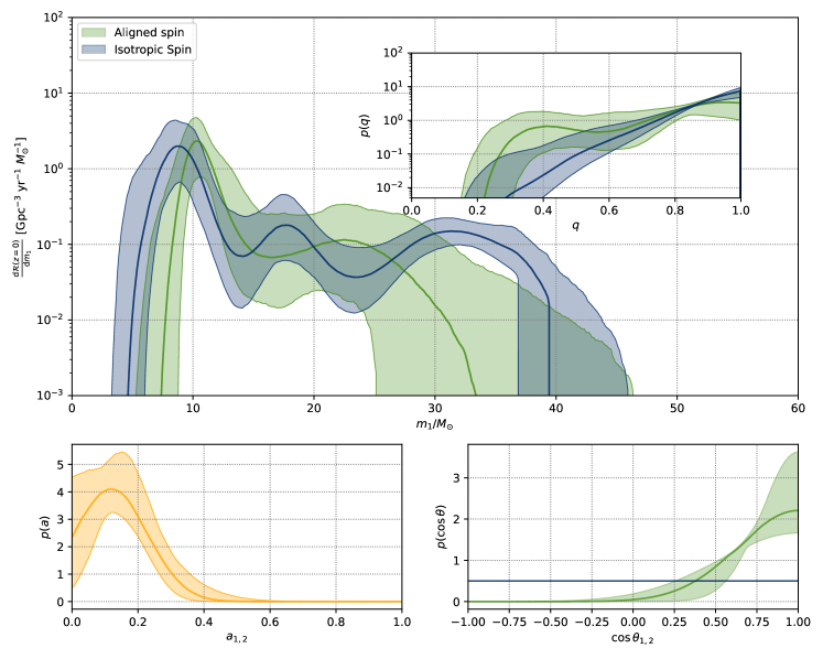
Figure 8: The same as Figure 6 but for the restriction of $\sigma_{\rm t}<0.5$.

B.3 Inference with a variable $\mu_{\rm t}$

Vitale et al. (2022) found no evidence for the $\cos\theta$ distribution peaking at $+1$. However, in Li et al. (2023), we found $\cos\theta$ distribution has strong preference for peaking at $+1$. Here, we have inferred with a variable $\mu_{\rm t}$ in the Extend Default. As show in Figure 10, the $\mu_{\rm t}$ peaks at $>0.5$, and $\mu_{\rm t}<0$ is strongly ruled out. Additionally, the mass and spin-magnitude distributions are unchanged, and the $\cos\theta$ distribution still has a preference for peaking at $+1$, as shown in Figure 9.

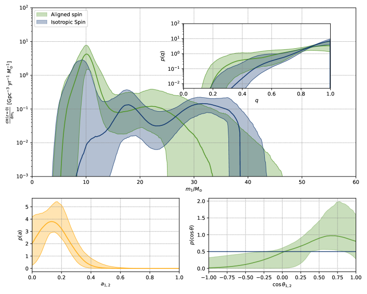
Figure 9: The same as Figure 6, but for the case with variable $\mu_{\rm t}$.

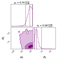
Figure 10: Posterior distributions of the $\mu_{\rm t}$ and $\sigma_{\rm t}$ describing the $\cos\theta_{1,2}$ distribution of the nearly-aligned subpopulation; the dashed lines in the marginal distribution represent the 90% credible intervals.

B.4 Is single nearly-aligned or isotropic-spin population also consistent with data?

Galaudage et al. (2021) found that the inferred spin distribution is nearly aligned, which is consistent with the hypothesis that all merging binaries form via the field formation scenario. To check out whether the a single nearly-aligned or a single isotropic-spin population is still satisfied by the current GW data, we infer with the single nearly-aligned model $M_{\rm A}$ and the single isotropic-spin model $M_{\rm I}$, which is expressed as

$$\pi_{\rm A}(\boldsymbol{\theta}|{\bf\Lambda})= \mathcal{PS}(m_{1},m_{2}|\alpha,\beta,\delta,m_{\rm min},m_{\rm max};f(m_{1}|\{x_{i}\},\{f_{i}\}))$$ (B1)

$$\times\mathcal{G}(\cos\theta_{1},\cos\theta_{2}|1,\sigma_{\rm t},-1,1)\times\mathcal{G}(a_{1},a_{2}|\mu_{\rm a},\sigma_{\rm a},0,1)\times p(z|\gamma=2.7),$$

and

$$\pi_{\rm I}(\boldsymbol{\theta}|{\bf\Lambda})= \mathcal{PS}(m_{1},m_{2}|\alpha,\beta,\delta,m_{\rm min},m_{\rm max};f(m_{1}|\{x_{i}\},\{f_{i}\}))$$ (B2)

$$\times\mathcal{U}(cos\theta_{1},\cos\theta_{2}|-1,1)\times\mathcal{G}(a_{1},a_{2}|\mu_{\rm a},\sigma_{\rm a},0,1)\times p(z|\gamma=2.7).$$

As shown in Table 2, the $M_{\rm I}$ is ruled out by a Bayes factor of $\ln\mathcal{B}=-5.5$, and the $M_{\rm A}$ is also slightly less favored compared to the Extend Default. However, if we restrict $\sigma_{\rm t}$ to be $<0.5$ as expected by the isolated field evolution (Rodriguez et al., 2016b), $M_{\rm A}$ was also rule out.

B.5 Inference with only $\cos{\theta_{1}}$

We also inferred with only $\cos\theta_{1}$ distribution, since $\cos\theta_{1}$ is usually constrained better than $\cos\theta_{2}$ in the parameter estimation for an individual event (Abbott et al., 2019, 2021a; The LIGO Scientific Collaboration et al., 2021a, b). As displayed in Figure 12, the results are nearly similar to that inferred in the main text. Figure 11 shows the posterior distribution of the main hyperparameter, we find $\sigma_{\rm t}=0.43^{+0.53}_{-0.26}$ is smaller than that inferred in the presence of $\cos\theta_{2}$, while other parameters are similar to those inferred with $\cos\theta_{2}$.

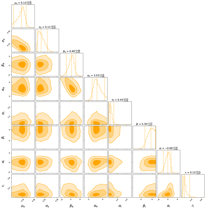
Figure 11: Posterior distribution of the main hyperparameter describing the two sub-populations, inferred without $\cos\theta_{2}$ information.

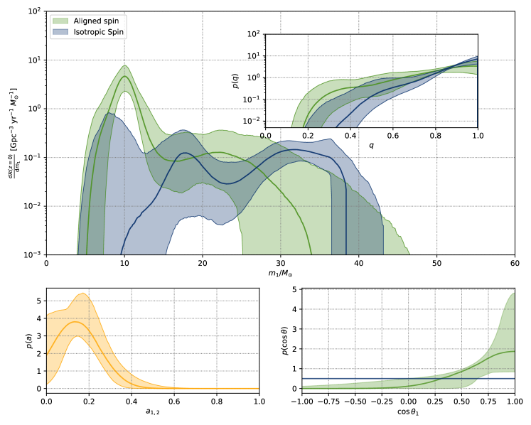
Figure 12: The same as Figure 6, but for the inference with only $\cos\theta_{1}$ distribution.

B.6 Is the spin-magnitude distributions of two sub-population identical?

To check out whether the spin-magnitudes of two sub-populations have the same distribution or significantly different distributions, we have also inferred with the model with two independent truncated Gaussian distributions to describe the spin-magnitude distributions of the two sub-populations, respectively.

$$\pi(\boldsymbol{\theta}|{\bf\Lambda})=[\mathcal{PS}(m_{1},m_{2} |\alpha_{\rm A},\beta_{\rm A},\delta_{\rm A},m_{\rm min,A},m_{\rm max,A};f_{\rm A}(m_{1}|\{x_{i}\},\{f_{i,{\rm A}}\}))$$ (B3)

$$\times \mathcal{G}(\cos\theta_{1},\cos\theta_{2}|1,\sigma_{\rm t},-1,1)\times\mathcal{G}(a_{1},a_{2}|\mu_{\rm a,A},\sigma_{\rm a,A},0,1)\times(1-r_{\rm I})$$

$$+\mathcal{PS}(m_{1},m_{2} |\alpha_{\rm I},\beta_{\rm I},\delta_{\rm I},m_{\rm min,I},m_{\rm max,I};f_{\rm I}(m_{1}|\{x_{i}\},\{f_{i,{\rm I}}\}))$$

$$\times \mathcal{U}(\cos\theta_{1},\cos\theta_{2}|-1,1)\times\mathcal{G}(a_{1},a_{2}|\mu_{\rm a,I},\sigma_{\rm a,I},0,1)\times r_{\rm I}]$$

$$\times p(z|\gamma=2.7).$$

As is shown in Figure 13, the spin magnitudes from the two sub-populations are nearly identical, and the Bayes factors (see Table 2) also show that the spin-magnitude distributions of the two sub-populations are not necessary to be different with current observation data.

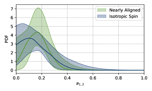
Figure 13: Spin-magnitude distributions of BBHs in the nearly-aligned and isotropic-spin sub-population. The solid curves are the medians and the colored bands are the 90% credible intervals.

Appendix C Classification

Table LABEL:tab:psub provides the probabilities of each first-generation event belonging to the field and dynamical channels. We find that the first detected BBH GW150914 (Abbott et al., 2016) originates from dynamical formation at $97.2\%$ credible level; while the popular asymmetric system GW190412 (Abbott et al., 2020b) is more likely to originate from field binary evolution, which was examined to be promised by Olejak et al. (2020). Additionally, the precession events GW190413_134308, GW200129_065458, and GW190521_074359 (Islam et al., 2023) are more likely originates from dynamical channel.

Table 4: Probabilities of the first-generation BBHs belonging to the field and dynamical sub-populations, inferred with the Extend Default model.

Events	Aligned	Isotropic
GW150914_095045	0.028	0.972
GW151012_095443	0.502	0.498
GW151226_033853	0.983	0.017
GW170104_101158	0.185	0.815
GW170608_020116	0.942	0.058
GW170809_082821	0.091	0.909
GW170814_103043	0.124	0.876
GW170818_022509	0.041	0.959
GW170823_131358	0.041	0.959
GW190408_181802	0.264	0.736
GW190412_053044	0.976	0.024
GW190413_134308	0.033	0.967
GW190421_213856	0.029	0.971
GW190503_185404	0.031	0.969
GW190512_180714	0.673	0.327
GW190513_205428	0.203	0.797
GW190521_074359	0.043	0.957
GW190527_092055	0.174	0.826
GW190630_185205	0.088	0.912
GW190707_093326	0.93	0.07
GW190708_232457	0.802	0.198
GW190720_000836	0.983	0.017
GW190727_060333	0.041	0.959
GW190728_064510	0.981	0.019
GW190803_022701	0.045	0.955
GW190828_063405	0.113	0.887
GW190828_065509	0.888	0.112
GW190910_112807	0.036	0.964
GW190915_235702	0.086	0.914
GW190924_021846	0.808	0.192
GW190925_232845	0.256	0.744
GW190930_133541	0.973	0.027
GW190413_052954	0.08	0.92
GW190719_215514	0.225	0.775
GW190725_174728	0.905	0.095
GW190731_140936	0.052	0.948
GW191105_143521	0.914	0.086
GW191127_050227	0.087	0.913
GW191129_134029	0.914	0.086
GW191204_171526	0.984	0.016
GW191215_223052	0.265	0.735
GW191216_213338	0.979	0.021
GW191222_033537	0.035	0.965
GW200112_155838	0.041	0.959
GW200128_022011	0.043	0.957
GW200129_065458	0.05	0.95
GW200202_154313	0.917	0.083
GW200208_130117	0.035	0.965
GW200209_085452	0.06	0.94
GW200219_094415	0.039	0.961
GW200224_222234	0.039	0.961
GW200225_060421	0.185	0.815
GW200302_015811	0.135	0.865
GW200311_115853	0.036	0.964
GW200316_215756	0.975	0.025
GW191103_012549	0.982	0.018
GW200216_220804	0.041	0.959

Appendix D Simulation of mock data

For the mock population with features found in this work, we assume the mass, spin, redshift distributions following Eq. D1 with $\alpha_{\rm A}=3.5$, $\beta_{\rm A}=1$, $\alpha_{\rm I}=0.5$, $\beta_{\rm I}=3$, $\delta^{\rm low}_{\rm A}=\delta^{\rm low}_{\rm I}=5M_{\odot}$, $m_{\rm min,A}=m_{\rm min,I}=5M_{\odot}$, $m_{\rm min,A}=m_{\rm min,I}=45M_{\odot}$, $\delta^{\rm high}_{\rm A}=\delta^{\rm high}_{\rm I}=10M_{\odot}$, $\sigma_{\rm t}=0.3$, $\mu_{\rm a}=0.15$, $\sigma_{\rm a}=0.1$, $r_{\rm I}=0.14$.

$$\pi(\boldsymbol{\theta}|{\bf\Lambda})=[\pi_{\rm A}(\boldsymbol{\theta}_{\rm d}|{\bf\Lambda}_{\rm A})\times(1-r_{\rm I})+\pi_{\rm I}(\boldsymbol{\theta}_{\rm d}|{\bf\Lambda}_{\rm I})\times r_{\rm I}]\times\pi_{\rm AI}(\boldsymbol{\theta}_{\rm s}|{\bf\Lambda}_{\rm AI})$$ (D1)

$$=[\mathcal{PL}(m_{1},m_{2}|\alpha_{\rm A},\beta_{\rm A},\delta_{\rm A},m_{\rm min,A},m_{\rm max,A},\delta_{\rm A}^{\rm high})\times \mathcal{G}(\cos\theta_{1},\cos\theta_{2}|1,\sigma_{\rm t},-1,1)\times(1-r_{\rm I})$$

$$+\mathcal{PL}(m_{1},m_{2}|\alpha_{\rm I},\beta_{\rm I},\delta_{\rm I},m_{\rm min,I},m_{\rm max,I},\delta_{\rm I}^{\rm high})\times \mathcal{U}(\cos\theta_{1},\cos\theta_{2}|-1,1)\times r_{\rm I}]$$

$$\times\mathcal{G}(a_{1},a_{2}|\mu_{\rm a},\sigma_{\rm a},0,1)\times p(z|\gamma=2.7)$$

the mass function of each subpopulation is

$$\mathcal{PL}(m_{1},m_{2}|{\bf\Lambda_{\rm m}})=C({\bf\Lambda_{\rm m}})m_{1}^{\alpha}~{}S(m_{1}|\delta^{\rm low},m_{\rm min},m_{\rm max},\delta^{\rm high})~{}m_{2}^{\alpha}~{}S(m_{2}|\delta^{\rm low},m_{\rm min},m_{\rm max},\delta^{\rm high})~{}(m_{2}/m_{1})^{\beta}~{}\Theta(m_{1}-m_{2}).$$ (D2)

with

$$S(m|\delta^{\rm low},m_{\rm min},m_{\rm max},\delta^{\rm high})=SL(m|m_{\rm min},\delta^{\rm low})SH(m|m_{\rm max},\delta^{\rm high})$$ (D3)

where $C({\bf\Lambda_{\rm m}})$ is the normalization factor, $\Theta(m_{1}-m_{2})$ denotes the Heaviside step function ensuring $m_{1}>m_{2}$, $SL(m|m_{\rm min},\delta^{\rm low})$ is the smooth function on the lower edge as introduced in Abbott et al. (2023), and $SH(m|m_{\rm max},\delta^{\rm high})$ is the smooth function on the upper edge which reads

$$\left\{\begin{aligned} &0&&(m>m_{\rm max}),\\ &[f(m_{\rm max}-m,\delta^{\rm high})+1]^{-1}&&(m_{\rm max}-\delta^{\rm high}<m<m_{\rm max}),\\ &1&&(m<m_{\rm max}-\delta^{\rm high})\end{aligned}\right.$$ (D4)

with

$$f(x,\delta^{\rm high})=\exp({\delta^{\rm high}}/{x}+{\delta^{\rm high}}/({x-\delta^{\rm high}}))$$ (D5)

For the mock population without features found in this work, we just assume the $\cos\theta$ of the two subpopulation following the same distribution as $\mathcal{GU}(\cos\theta_{1},\cos\theta_{2}|\sigma_{\rm t},\zeta)=\mathcal{G}(\cos\theta_{1},\cos\theta_{2}|1,\sigma_{\rm t},-1,1)\times\zeta+\mathcal{U}(\cos\theta_{1},\cos\theta_{2}|-1,1)\times(1-\zeta)$, (i.e., the Default spin-orientation model in Abbott et al. (2023),) with $\sigma_{\rm t}=0.3$ and $\zeta=0.5$. Therefore the mass, spin, redshift distributions read

$$\pi(\boldsymbol{\theta}|{\bf\Lambda})=[\mathcal{PL}(m_{1},m_{2}|\alpha_{\rm A},\beta_{\rm A},\delta_{\rm A},m_{\rm min,A},m_{\rm max,A},\delta_{\rm A}^{\rm high})\times(1-r_{\rm I})$$ (D6)

$$+\mathcal{PL}(m_{1},m_{2}|\alpha_{\rm I},\beta_{\rm I},\delta_{\rm I},m_{\rm min,I},m_{\rm max,I},\delta_{\rm I}^{\rm high})\times r_{\rm I}]$$

$$\times\mathcal{GU}(\cos\theta_{1},\cos\theta_{2}|\sigma_{\rm t},\zeta)\times\mathcal{G}(a_{1},a_{2}|\mu_{\rm a},\sigma_{\rm a},0,1)\times p(z|\gamma=2.7)$$

The mass and spin-orientation distributions are the same as those of the mock population with features, i.e., $\alpha_{\rm A},\beta_{\rm A},\delta_{\rm A},m_{\rm min,A},m_{\rm max,A},\delta_{\rm A}^{\rm high},\alpha_{\rm I},\beta_{\rm I},\delta_{\rm I},m_{\rm min,I},m_{\rm max,I},\delta_{\rm I}^{\rm high},\mu_{\rm a},\sigma_{\rm a}$ are set the same as those in Eq. D1.

To generate the detected events of the mock population we randomly choose events from the injection campaign for O3 Search Sensitivity Estimates with the inverse False Alarm Rate $>1{\rm yr}$, each event is assigned a draw weight proportional to $p(\boldsymbol{\theta}|{\bf\Lambda})/p_{\rm draw}(\boldsymbol{\theta})$, where $p(\boldsymbol{\theta}|{\bf\Lambda})$ is the probability distribution of mock population, and $p_{\rm draw}(\boldsymbol{\theta})$ is the probability distribution from which the injection campaigns are drawn. For each mock population, we adopt 57 detections, similar to the size of the first-generation BBHs in the real data of GWTC-3. With each mock detection, we then use IMRPhenomXPHM waveform (Pratten et al., 2021) to generate GW signal and inject it to the noise generated by the “O3 actual” noise power spectral densities. We perform parameter estimation on each event using BILBY (Ashton et al., 2019) with the NESSAI (Williams et al., 2021) nested sampler.

Then we use the model (Eq. 5) introduced in the main text, to respectively infer the underlying distribution of the two mock populations. Figure 15 / Figure 14 shows the recovered distributions of the mock population with / without the features of spin-orientation distributions found in this work.

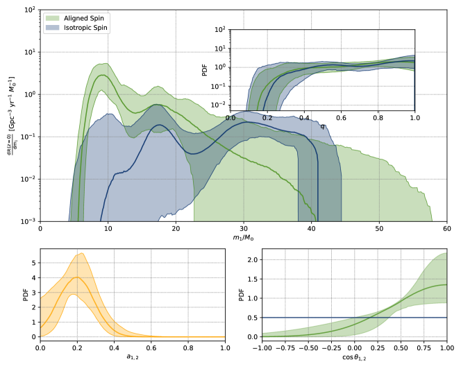
Figure 14: The same as Fig. 6, but for the analysis with mock data where the injections having features found in this work.

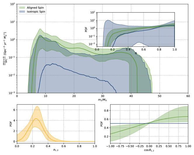
Figure 15: The same as Fig. 14, but for injections do not have features found in this work.

Appendix E Comparison with BHs in HMXBs

Fishbach & Kalogera (2022) firstly compared the BHs in XRBs with those in GW sources, and concluded that the two types of BHs are ‘Apple and Orange’, for the significant disagreement in their spin-magnitude distributions, though the mass distributions are still consistent. Anyway, the GW sources may originate from several channels, and the higher-generation BHs in hierarchical mergers are unlikely to be the same as the BHs in XRBs (Fishbach et al., 2017; Li et al., 2023). Therefore, it would be more appropriate to compare the BHs from ‘Apple to Apple’, i.e., comparing the BHs from one individual formation channel we inferred with the BHs in XRBs. Here, we focus on comparing GW sources with BHs in HMXBs. This is because HMXBs are more likely to be the progenitors of merging BBHs due to the presence of massive mass donor. Figure 16 (left) compares the primary-mass distribution of the field BBHs to the mass distribution of HMXB BHs . The green dashed region is the inferred primary-mass cumulative distribution function (CDF) of the field-evolution BBHs, while the blue dashed region is the predicted CDF of 3 random draws from the field-evolution BBH primary mass distribution. We find that the HMXB BHs are slightly heavier than the BHs in the Field BBHs, though the mass distribution of the HMXB BHs and the 3 predicted BBHs are still consistent within the Poisson uncertainty.

The spin-magnitude distribution of the BBHs inferred with our model ($\mu_{\rm a}=0.11^{+0.06}_{-0.09}$, $\sigma_{\rm a}=0.12^{+0.07}_{-0.05}$) is significantly in disagreement with the spin magnitudes of the HMXB BHs (Reynolds, 2021), such a result was also found in the comparison between the full BBH catalog and the HMXB BHs by Fishbach & Kalogera (2022). Considering the differences in the mass functions and spin-magnitude distributions between the field-evolution BBHs and the HMXB BHs, it is possible that the HMXB BHs may have accreted significant mass, e.g., the BH mass can increase by a factor of 1.3 (Gallegos-Garcia et al., 2022; Shao & Li, 2022); simultaneously, BHs are spun up by super-Eddington accretion under the assumption of conservative mass transfer (MT) (Qin et al., 2022; Shao & Li, 2022). Conservative MT widens the orbits of the HMXBs and hence prevents them from merger within a Hubble time (Bavera et al., 2021; Zevin & Bavera, 2022), which lead to wide BBHs or wide neutron star-BHs (Gallegos-Garcia et al., 2022). This scenario is also consistent with the fact that HMXBs have been observed yet are not expected to merge within the Hubble time (Belczynski et al., 2011, 2012; Neijssel et al., 2021; Gallegos-Garcia et al., 2022).

We also compared the mass function of the BHs in dynamical channels to the HMXB BHs, as shown in Figure 16 (right). The masses of the HMXB BHs are smaller than BHs in the dynamical channel (pale-green regions). However, when we modified the dynamical-channel mass function with $\alpha=\alpha_{\rm I}+2$ to mimic the initial mass function of BHs in the environments of dynamical channels (O’Leary et al., 2016), the initial mass function (sandy-brown regions) seems consistent with the HMXB BHs.

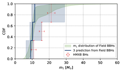
Figure 16: Masses of the three observed HMXB BHs (red error bars), compared to the mass function of field BBHs (left) and dynamical BBHs (right) from GW population inference. Left: the green dashed region shows the 90% credible interval of the inferred primary-mass function of field BBHs; the blue lines and dashed regions show the median and 90% credible intervals of the CDF curves of three random draws from the field BBH primary-mass distribution. Right: the pale-green regions are the inferred mass function of dynamical BBHs, while the sandy-brown regions are the modified mass function of dynamical BBHs with $\alpha=\alpha_{\rm I}+2$, indicating the initial mass function of BHs in the environment for dynamical channels (O’Leary et al., 2016).

References

- Abbott et al. (2016) Abbott, B. P., Abbott, R., Abbott, T. D., et al. 2016, Phys. Rev. Lett., 116, 061102, doi: 10.1103/PhysRevLett.116.061102
- Abbott et al. (2017) —. 2017, Phys. Rev. Lett., 119, 161101, doi: 10.1103/PhysRevLett.119.161101
- Abbott et al. (2018) —. 2018, Living Reviews in Relativity, 21, 3, doi: 10.1007/s41114-018-0012-9
- Abbott et al. (2019) —. 2019, Physical Review X, 9, 031040, doi: 10.1103/PhysRevX.9.031040
- Abbott et al. (2020a) —. 2020a, ApJ, 892, L3, doi: 10.3847/2041-8213/ab75f5
- Abbott et al. (2020b) Abbott, R., Abbott, T. D., Abraham, S., et al. 2020b, Phys. Rev. D, 102, 043015, doi: 10.1103/PhysRevD.102.043015
- Abbott et al. (2021a) —. 2021a, Physical Review X, 11, 021053, doi: 10.1103/PhysRevX.11.021053
- Abbott et al. (2021b) —. 2021b, ApJ, 915, L5, doi: 10.3847/2041-8213/ac082e
- Abbott et al. (2021c) —. 2021c, ApJ, 913, L7, doi: 10.3847/2041-8213/abe949
- Abbott et al. (2022) Abbott, R., Abbott, T. D., Acernese, F., et al. 2022, A&A, 659, A84, doi: 10.1051/0004-6361/202141452
- Abbott et al. (2023) —. 2023, Physical Review X, 13, 011048, doi: 10.1103/PhysRevX.13.011048
- Antonini et al. (2023) Antonini, F., Gieles, M., Dosopoulou, F., & Chattopadhyay, D. 2023, MNRAS, 522, 466, doi: 10.1093/mnras/stad972
- Antonini et al. (2019) Antonini, F., Gieles, M., & Gualandris, A. 2019, MNRAS, 486, 5008, doi: 10.1093/mnras/stz1149
- Ashton et al. (2019) Ashton, G., Hübner, M., Lasky, P. D., et al. 2019, Bilby: Bayesian inference library, Astrophysics Source Code Library, record ascl:1901.011. http://ascl.net/1901.011
- Baibhav et al. (2023) Baibhav, V., Doctor, Z., & Kalogera, V. 2023, ApJ, 946, 50, doi: 10.3847/1538-4357/acbf4c
- Banerjee (2017) Banerjee, S. 2017, MNRAS, 467, 524, doi: 10.1093/mnras/stw3392
- Bavera et al. (2021) Bavera, S. S., Fragos, T., Zevin, M., et al. 2021, A&A, 647, A153, doi: 10.1051/0004-6361/202039804
- Belczynski et al. (2011) Belczynski, K., Bulik, T., & Bailyn, C. 2011, ApJ, 742, L2, doi: 10.1088/2041-8205/742/1/L2
- Belczynski et al. (2012) Belczynski, K., Bulik, T., & Fryer, C. L. 2012, arXiv e-prints, arXiv:1208.2422, doi: 10.48550/arXiv.1208.2422
- Belczynski et al. (2010) Belczynski, K., Bulik, T., Fryer, C. L., et al. 2010, ApJ, 714, 1217, doi: 10.1088/0004-637X/714/2/1217
- Belczynski et al. (2021) Belczynski, K., Done, C., & Lasota, J. P. 2021, arXiv e-prints, arXiv:2111.09401, doi: 10.48550/arXiv.2111.09401
- Buchner (2016) Buchner, J. 2016, PyMultiNest: Python interface for MultiNest, Astrophysics Source Code Library, record ascl:1606.005. http://ascl.net/1606.005
- Cai et al. (2018) Cai, Y.-F., Tong, X., Wang, D.-G., & Yan, S.-F. 2018, Phys. Rev. Lett., 121, 081306, doi: 10.1103/PhysRevLett.121.081306
- Callister et al. (2021) Callister, T. A., Haster, C.-J., Ng, K. K. Y., Vitale, S., & Farr, W. M. 2021, ApJ, 922, L5, doi: 10.3847/2041-8213/ac2ccc
- Callister et al. (2022) Callister, T. A., Miller, S. J., Chatziioannou, K., & Farr, W. M. 2022, ApJ, 937, L13, doi: 10.3847/2041-8213/ac847e
- Cheng et al. (2023) Cheng, A. Q., Zevin, M., & Vitale, S. 2023, ApJ, 955, 127, doi: 10.3847/1538-4357/aced98
- de Mink & Mandel (2016) de Mink, S. E., & Mandel, I. 2016, MNRAS, 460, 3545, doi: 10.1093/mnras/stw1219
- Edelman et al. (2022) Edelman, B., Doctor, Z., Godfrey, J., & Farr, B. 2022, ApJ, 924, 101, doi: 10.3847/1538-4357/ac3667
- Essick et al. (2022) Essick, R., Farah, A., Galaudage, S., et al. 2022, ApJ, 926, 34, doi: 10.3847/1538-4357/ac3978
- Essick & Farr (2022) Essick, R., & Farr, W. 2022, arXiv e-prints, arXiv:2204.00461, doi: 10.48550/arXiv.2204.00461
- Farr et al. (2018) Farr, B., Holz, D. E., & Farr, W. M. 2018, ApJ, 854, L9, doi: 10.3847/2041-8213/aaaa64
- Farr (2019) Farr, W. M. 2019, Research Notes of the American Astronomical Society, 3, 66, doi: 10.3847/2515-5172/ab1d5f
- Fishbach et al. (2020) Fishbach, M., Essick, R., & Holz, D. E. 2020, ApJ, 899, L8, doi: 10.3847/2041-8213/aba7b6
- Fishbach & Holz (2020) Fishbach, M., & Holz, D. E. 2020, ApJ, 891, L27, doi: 10.3847/2041-8213/ab7247
- Fishbach et al. (2017) Fishbach, M., Holz, D. E., & Farr, B. 2017, ApJ, 840, L24, doi: 10.3847/2041-8213/aa7045