Reconstructing Curves from Sparse Samples on Riemannian Manifolds

Abstract

Reconstructing 2D curves from sample points has long been a critical challenge in computer graphics, finding essential applications in vector graphics. The design and editing of curves on surfaces has only recently begun to receive attention, primarily relying on human assistance, and where not, limited by very strict sampling conditions. In this work, we formally improve on the state-of-the-art requirements and introduce an innovative algorithm capable of reconstructing closed curves directly on surfaces from a given sparse set of sample points. We extend and adapt a state-of-the-art planar curve reconstruction method to the realm of surfaces while dealing with the challenges arising from working on non-Euclidean domains. We demonstrate the robustness of our method by reconstructing multiple curves on various surface meshes. We explore novel potential applications of our approach, allowing for automated reconstruction of curves on Riemannian manifolds.

<ccs2012> <concept> <concept_id>10002950.10003624.10003633.10003640</concept_id> <concept_desc>Mathematics of computing Paths and connectivity problems</concept_desc> <concept_significance>500</concept_significance> </concept> <concept> <concept_id>10002950.10003624.10003633.10010917</concept_id> <concept_desc>Mathematics of computing Graph algorithms</concept_desc> <concept_significance>300</concept_significance> </concept> <concept> <concept_id>10010147.10010371.10010396.10010398</concept_id> <concept_desc>Computing methodologies Mesh geometry models</concept_desc> <concept_significance>300</concept_significance> </concept> </ccs2012>

[500]Mathematics of computing Paths and connectivity problems [300]Mathematics of computing Graph algorithms [300]Computing methodologies Mesh geometry models

1 Introduction

Vector graphics represents an important research area in computer graphics, and it is widely applied in many fields, spanning from design and art to engineering. One of the important reasons for its success is the ability to generate infinite resolution smooth complex visualizations with relative ease while requiring only little input geometry.

Recently, an increasing interest has been devoted to moving 2D vector graphics onto surfaces, trying to address certain issues stemming from texturing methods. Texturing is a well-established approach for defining patterns and decorations on surfaces, but it generally relies on finite-resolution images and parameterization. The latter is not always available or could be difficult or expensive to define. Procedural textures try to overcome these problems, defining patterns via mathematical functions and algorithms. However, they generally rely on multi-dimensional noise functions that are then sampled on the surface [EMP^∗03, Har01, MBMR22]. These algorithms are usually agnostic of the underlying geometric properties and can incur high computation times.

Besides works generalizing sample-based texture synthesis to triangular meshes [WL01, Tur01], only in recent years some solutions have been proposed which try to leverage properties of non-Euclidean metric spaces and define patterns directly on surfaces, either via recursive structures [NPP21] or simulated behaviors [MMMR22]. Another avenue of development for texture synthesis is represented by neural networks that generate a textured mesh in the style of an input image [MG23].

Despite the existence of various solutions for decorating surfaces, the problem of constructing lines and curves on discrete manifolds has not been addressed satisfactorily yet. Defining curves and shapes directly on surfaces is innovative for design applications [PSOA18], and has a relevant impact in the processing of archaeological data [KST08, GTSK13] by extracting specific decorations from the models. However, little research has been devoted to improving the definition and the reconstruction of curves on discrete surfaces, besides efforts to generalize Bézier curves [MNPP21]. Furthermore, the existing techniques are generally centered around human interaction, as they are designed to be tools for artists and end users, and even the most recent solutions require an ordered sequence of samples [MP23]. To the best of our knowledge, Shah et al. [SC13] provided the first and only solution for dealing with curve reconstruction on Riemannian manifolds. Still, their proposed method can only deal with dense uniform samplings and only guarantees to reconstruct curves in limited settings. By generalizing state-of-the-art theoretical results and algorithmic solutions for planar curve reconstruction to arbitrary manifold domains, we introduce a more robust method that, given an unordered collection of points over a Riemannian manifold that follows our relaxed sampling conditions, always produces an ordered sequence identifying a closed curve on the surface (see Reconstructing Curves from Sparse Samples on Riemannian Manifolds).

Our contributions are summarized in the following:

• we propose a solution that extends existing state-of-the-art theory and techniques for 2D curve reconstruction to manifold domains, overcoming the challenges arising from translating the problem into non-Euclidean spaces;

• we improve the state-of-the-art sampling conditions for curve reconstruction on Riemannian manifolds [SC13], allowing for sparser sampling for curve reconstruction on manifold domains;

• we perform a qualitative study of our method on real-world data coming from established applications, where the previous solution fails due to the sparsity of the samples.

2 Related work

Reconstructing curves from samples in a non-Euclidean space extends the classical problem of planar curve reconstruction to more complex spaces, drawing inspiration from tangent domains: surface design and texturing using on-surface elements. This section will provide an overview of various techniques that deal with each of these fields individually and explain how they relate to our work.

Planar curve reconstruction, where the input samples and their respective reconstructed curve live in $\mathbb{R}^{2}$, is dealt with by numerous methods. They are usually divided into two main categories: implicit (methods that approximate the inside/outside of the shape and recreate the boundary based on the division between the two) [HDD^∗92, KBH06] and explicit (interpolatory methods that create some ordering among the sample points). We will focus on the explicit reconstruction methods, as they are the most relevant to our work. However, most of these methods are limited to planar curves, with some of them extended to reconstructing surfaces as well. Some of the presented methods can reconstruct curves in $\mathbb{R}^{3}$ but the samples do not live on a manifold.

To interpolate the input sample points, most methods compute a graph on the input and use a subset of the edges as the final reconstruction. One of the most commonly used types of graphs is the Delaunay triangulation, due to its geometrical properties and theoretical guarantees of including the reconstruction subject to sampling density [ABE98]. Starting from the Delaunay triangulation, Amenta et al. filter the edges whose proximity is empty of samples and of Voronoi vertices. This approach has been improved to take into account Voronoi poles - Voronoi vertices corresponding to long, skinny Voronoi cells [ACK01].

Using the same Delaunay starting base, a greedy procedure is used to pick a seed vertex and find the nearest neighbors until the endpoints are close enough to be connected or until all points have been connected [PM16]. Similarly, various criteria have been devised for keeping a Delaunay edge between two points: the new neighbor has to be situated in the half-plane (defined using the normal at the current sample) opposite to the previous connection [DK99], or in the opposite half-plane defined using the bisector of the previous edge [OMW16]. Another set of criteria used to filter the triangulation is based on leveraging the Voronoi poles to approximate the normals for the half-plane computation, considering the angle and the ratio between the current edge and its Voronoi counterpart [DW02]. Various other methods build on the Delaunay triangulation as a starting base for curve reconstruction [OM13, MOW22], and a comprehensive survey on multiple implicit methods can be found here [OPP^∗21]. Our method lifts the reconstruction of curves from planar surfaces to manifold domains of any dimension.

Curve reconstruction on Riemannian manifolds has been approached as an extension of planar metrics and sampling conditions to Riemannian manifolds [SC13]. However, the classical definition of the medial axis does not hold on surfaces if the medial axis is constrained to live on the surface as well. The authors introduce a new sampling criterion, based on the minimum value between the distance to the medial axis and the injectivity radius. We introduce the formal definitions of these concepts in Section 3 and we relax their dense sampling requirements in Section 4 to allow for reconstruction with fewer samples. To the best of our knowledge, this is the only work that extends the problem of curve reconstruction to Riemannian manifolds.

Vector graphics on planar surfaces have been thoroughly researched and are being used in multiple tools [Ink, Ado]. Recently, editing and importing curves on surfaces have received interest in the graphics field, partly due to the improvement in computing geodesic paths efficiently [SC20]. Users can interact with designs directly on the mesh, by either editing splines on a 2D local projection of the surface [PSOA18], which is usually prone to artifacts due to the projection procedure, as explored in [YLT19], or editing splines directly on the surfaces, bypassing the projection artifacts, by using geodesic metrics on the surface [NPP21, MNPP21]. However, these editing methods require user input or a predefined ordering of the samples to construct the curves on the surface, which is the missing link we are providing. Hence, our method also provides a building block for further editing splines on surfaces.

3 Background and notations

Informally speaking, a $d$-dimensional manifold is a collection of pieces of the $d$-dimensional hyperspace that are deformed and glued together to form a continuous smooth domain. Such domain can be embedded in a higher dimensional space (like in the case of 2-dimensional surfaces embedded in 3D space), or exist on their own (like the 3D rotation group $\mathrm{SO}(3)$ [HH13]). For a formal and complete definition of Riemannian manifolds, we refer to the books from Morita and Do Carmo [Mor01, DC16].

For referring to any such $d$-dimensional manifold (including continuous curves) we use calligraphic letters (i.e., $\mathcal{M}$, $\mathcal{C}$), and we denote the geodesic distance function over a manifold $\mathcal{M}$ with $d_{\mathcal{M}}$. Furthermore, we refer to any discrete representation of a manifold $\mathcal{M}$ with the symbol $\hat{\mathcal{M}}$.

Specifically, we represent discrete $2$-dimensional surfaces as triplets $\hat{\mathcal{M}}=(V,E,T)$, where $V$ is a set of vertices, $T$ is a set of oriented triangles among vertices, and $E$ is a set of unordered edges induced by the triangles in $T$. We also represent discrete curves (i.e., 1-dimensional manifolds) as tuples $\hat{\mathcal{C}}=(V,E)$, where $V$ is a set of vertices and $E$ is a set of edges between vertices. Throughout this work, we assume the manifoldness of discrete surfaces and curves [CDGDS13], and we assume to work with curves made by a single component and forming a closed non-self-intersecting loop.

We also recall the definitions of medial axis and local feature size (see Figure 1), which we will use for distinguishing between different curve sampling strategies.

Definition 1 ([Blu67]).

Let $\mathcal{C}$ be a smooth curve embedded in a metric space $(\mathcal{M},d_{\mathcal{M}})$. The medial axis $\Gamma(\mathcal{C})$ of $\mathcal{C}$ is the closure of the set of points in $\mathcal{M}$ that have two or more closest points in $\mathcal{C}$.

Definition 2 ([Rup93]).

Let $p\in\mathcal{C}$ be a point on the curve. The local feature size $\mathrm{lfs}({p})$ of $p$ is the minimum distance from $p$ to the medial axis of $\mathcal{C}$.

$$\mathrm{lfs}({p})=\min_{q\in\Gamma(\mathcal{C})}d_{\mathcal{M}}(p,q)\,.$$ (1)

3.1 Curve sampling

In this section, we repeat definitions related to sampling planar curves and conclude with our own definitions that extend to manifolds.

Given a smooth curve $\mathcal{C}$ and a set of samples $S\subset\mathcal{C}$, reconstructing the curve is the process of constructing a discrete curve $\hat{\mathcal{C}}=(S,E)$ such that an edge $e=(s_{i},s_{j})$ is in $E$ if and only if $s_{i}$ and $s_{j}$ are consecutive samples along the curve $\mathcal{C}$.

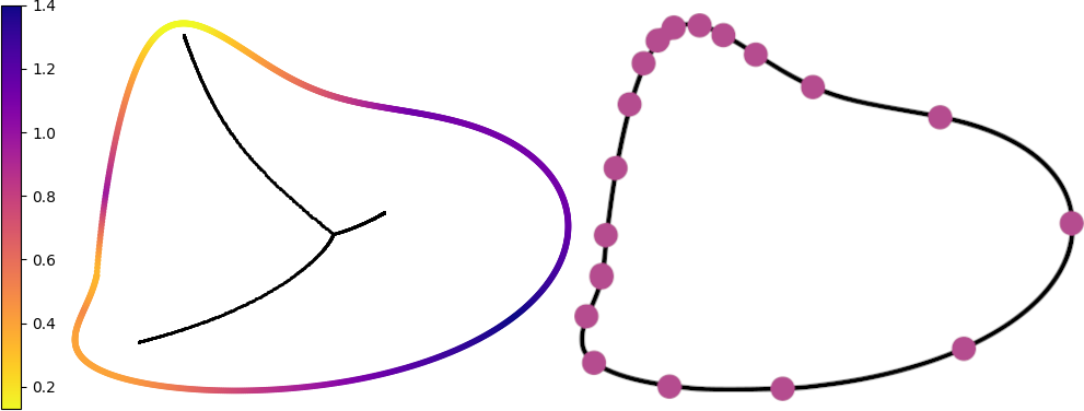
Figure 1: Left: the local feature size at each point of the curve represents its distance to the medial axis (in black). Right: a $\rho$-sampling of the curve with $\rho=1.0$ shows that the samples are denser where the medial axis is closer to the curve.

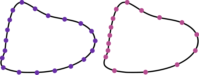
Figure 2: Difference between uniform sampling (left) and non-uniform sampling (right) with non-uniformity ratio $u=1.5$.

One technique to evaluate the sampling quality is by using the $\rho$ value, which was introduced by Ohrhallinger et al. [OMW16] and relies on the notion of reach.

Definition 3 ([Fed59]).

The reach of an interval $I\subset\mathcal{C}$ is the minimum local feature size among points in the interval:

$$\mathrm{reach}({I})=\inf_{p\in I}\ \mathrm{lfs}({p})\,.$$ (2)

Definition 4 ([OMW16]).

A smooth curve $\mathcal{C}$ is $\rho$-sampled by a sample set $S\subset\mathcal{C}$ if every point $p\in\mathcal{C}$ of the curve is closer to a sample than a $\rho$-fraction of the reach of the interval $I=[s_{0},s_{1}]$ of consecutive samples containing it:

$$\forall p\in I,\ \min_{s\in\{s_{0},s_{1}\}}\ d_{\mathcal{M}}(p,s)<\rho\ \mathrm{reach}({I})\,.$$ (3)

In Figure 1, we show how the $\rho$-sampling depends on the local feature size, requiring a more dense sampling where the medial axis is closer to the curve and allowing a more sparse sampling where the local feature size is larger.

A different category of sampling conditions enforces a specific distance between consecutive samples, unrelated to the medial axis. Hence, we conclude our collection of planar sampling conditions by distinguishing between uniform and non-uniform sampling, examples of which can be observed in Figure 2.

Definition 5.

A smooth curve $\mathcal{C}$ is uniformly $\vartheta$-sampled by a sample set $S\subset\mathcal{C}$ if for any two consecutive samples $s_{0},s_{1}\in S$, it holds $d_{\mathcal{M}}(s_{0},s_{1})<\vartheta$.

Definition 6.

A smooth curve $\mathcal{C}$ is non-uniformly sampled with a non-uniformity ratio $u\in\mathbb{R}^{+}$ by a sample set $S\subset\mathcal{C}$ if for any three consecutive samples $s_{0},s_{1},s_{2}\in S$, it holds that $u_{s_{1}}<u$, where the $u_{s_{1}}$ is defined as:

$$u_{s_{1}}=\frac{\max\left(d_{\mathcal{M}}(s_{0},s_{1}),d_{\mathcal{M}}(s_{1},s_{2})\right)}{\min\left(d_{\mathcal{M}}(s_{0},s_{1}),d_{\mathcal{M}}(s_{1},s_{2})\right)}\,.$$ (4)

3.2 Differential geometry

We now lift the definitions required for the local feature size from the plane to manifolds, to be able to introduce sampling conditions on manifolds in the subsequent sections.

Euclidean disks are widely used in relation to planar curve reconstruction, and they have a straightforward generalization to arbitrary metric spaces.

Definition 7.

Let $(\mathcal{M},d_{\mathcal{M}})$ be a metric space, $p\in\mathcal{M}$ a point on $\mathcal{M}$, and $r\in\mathbb{R}$. The $r$-ball centered at $p$ is the region $\mathcal{B}_{{p},{r}}$ of points at a distance less than $r$ from $p$:

$$\mathcal{B}_{{p},{r}}=\left\{x\in\mathcal{M}\ :\ d_{\mathcal{M}}(p,x)<r\right\}\,.$$ (5)

The closure $\mathrm{cl}{\mathcal{B}_{{p},{r}}}$ of the $r$-ball also includes its boundary:

$$\partial\mathcal{B}_{{p},{r}}=\left\{x\in\mathcal{M}\ :\ d_{\mathcal{M}}(p,x)=r\right\}\,.$$ (6)

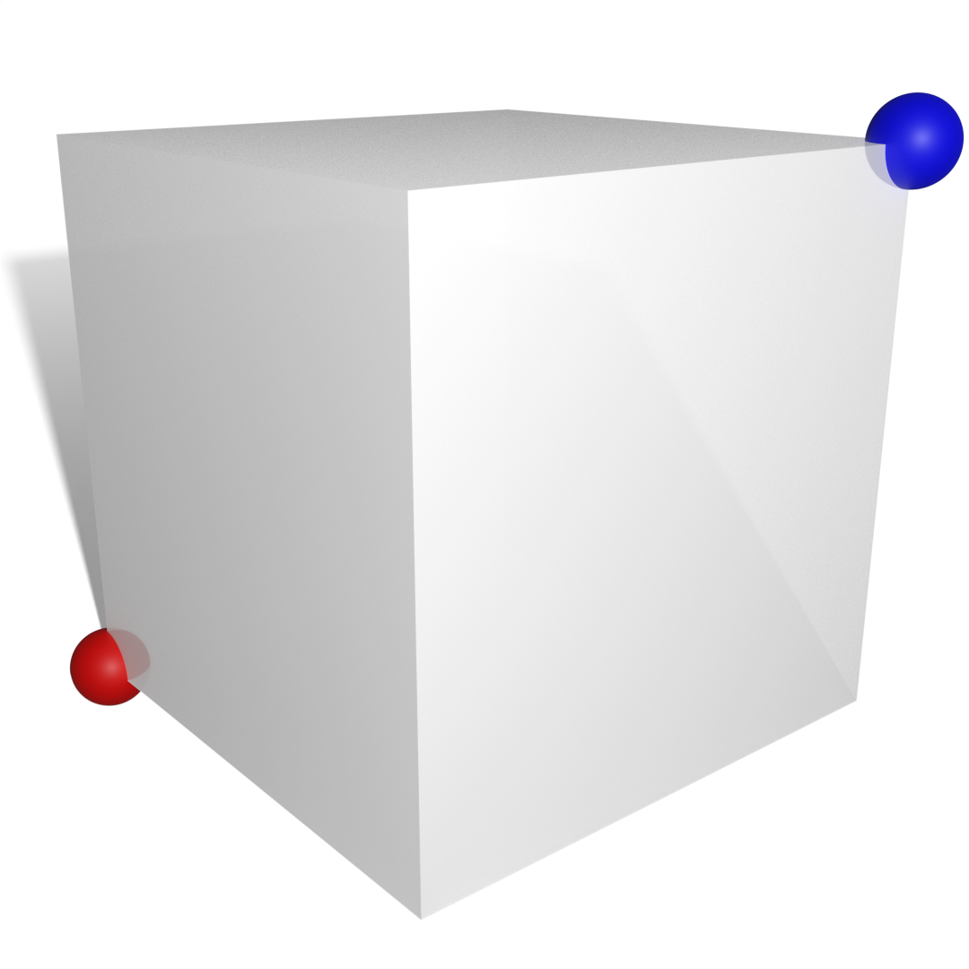
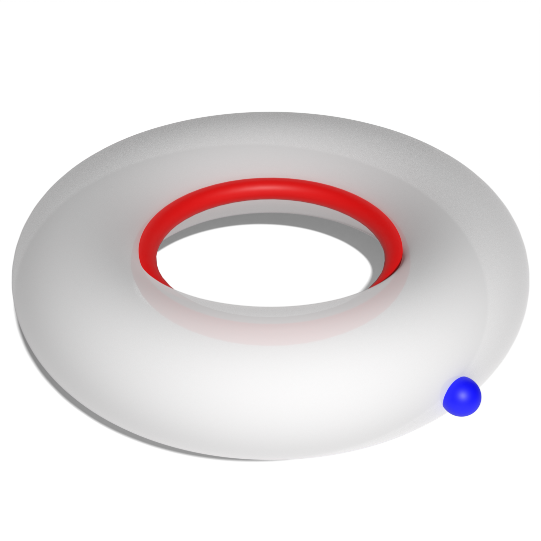
Figure 3: Examples of cut locus (in red) given a point (in blue) on different surfaces. The cut locus can be a single point (left) or an entire curve (right).

The work of Shah et al. [SC13] identifies the limitations of the local feature size in non-Euclidean metric spaces, and exploits the notions of cut locus and injectivity radius to overcome these issues.

Definition 8.

Let $\mathcal{M}$ be a $d$-dimensional Riemannian manifold, possibly with boundary $\partial\mathcal{M}$, and equipped with a connection defining an exponential map $\exp_{p}:T_{p}(\mathcal{M})\to\mathcal{M}$ at every point $p\in\mathcal{M}$. The cut locus of $p$ in the tangent space $T_{p}(\mathcal{M})$ is defined as the set $C_{T(\mathcal{M})}(p)$ of all vectors $v\in T_{p}(\mathcal{M})$ such that the parametric curve $\exp_{p}(tv)$ is a minimizing geodesic for $t\in[0,1]$ and not minimizing for $t>1$.

The cut locus of $p$ on the manifold $\mathcal{M}$ is the set $C_{\mathcal{M}}(p)$ of all points $q\in\mathcal{M}$ that are the image of a vector $v\in C_{T(\mathcal{M})}$ under the exponential map.

Informally speaking, the cut locus of a point $p$ on the manifold $\mathcal{M}$ can be seen as the set of all points $q$ such that there are at least two distinct minimizing geodesics from $p$ to $q$ – see Figure 3.

Definition 9 ([DC16]).

Let $p\in\mathcal{M}$ be a point on the manifold $\mathcal{M}$ and $C_{\mathcal{M}}(p)$ be its cut locus. The injectivity radius of $p$ is

$$i_{\mathcal{M}}(p)=\inf_{q\in C_{\mathcal{M}}(p)}d_{\mathcal{M}}(p,q)\,.$$ (7)

The injectivity radius of the manifold $\mathcal{M}$ is thus defined as

$$\mathfrak{I}_{\mathcal{M}}=\inf_{p\in\mathcal{M}}i_{\mathcal{M}}(p)\,.$$ (8)

By using these tools, Shah et al. [SC13] show that curves can be reconstructed using a minimum spanning tree, if they are uniformly $\vartheta$-sampled, with $\vartheta<\min\left(\inf_{p\in\mathcal{C}}\mathrm{lfs}({p}),\mathfrak{I}_{\mathcal{M}}\right)$.

4 Method

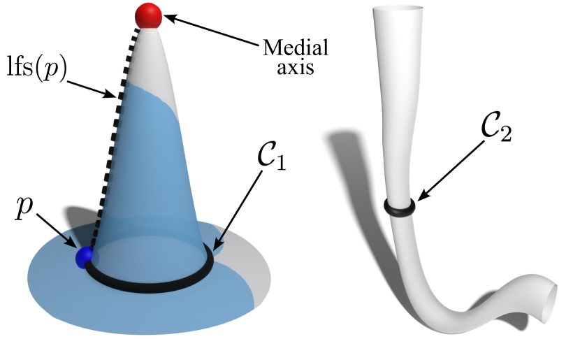
Figure 4: Two examples of curves on surfaces (solid black) where the local feature size exhibits undesired behaviors. Left: an $r$-ball (shaded in light blue) around $p$ that contains the entire curve $\mathcal{C}_{1}$, but no point of the medial axis. Right: a curve $\mathcal{C}_{2}$ on the surface with an empty medial axis (i.e., the local feature size is undefined).

In this paper, we advance the task of reconstructing curves on manifolds, addressing curves that are sampled more sparsely and non-uniformly compared to the state-of-the-art.

The standard notion of local feature size is not suitable for non-Euclidean metric spaces. In Figure 4 we show two examples of curves where the local feature size presents undesired behaviors. For instance, we can have $r$-balls that contain the entire curve without containing the medial axis, or even curves that do not have a medial axis, making it impossible to define the local feature size.

By taking inspiration from Shah et al. [SC13], we exploit the injectivity radius to strengthen the definition of $\rho$-sampling, making it suitable for manifold domains and showing that we can preserve its fundamental properties (Section 4.1). Then, we generalize a proximity graph successfully used for 2D curve reconstruction to arbitrary metric spaces, proving that analogous sampling conditions apply (Section 4.2). And finally, we present an algorithm that relies on the properties of our graph to reconstruct curves on Riemannian manifolds (Section 4.3). The proofs of all our claims are provided in Appendix A.

4.1 Non-uniform sparse sampling on surfaces

The solution proposed by Shah et al. [SC13] consists of bounding the local feature size to the injectivity radius of the entire surface. While this approach effectively solves the previous issues, it also makes the sampling very dense when the manifold contains very narrow sections or sharp features: the smallest injectivity radius of the surface affects the overall sampling conditions, even if the curve might not pass close to these regions. Instead, we use the local feature size and the reach by considering the injectivity radius of individual points.

Definition 10.

Let $\mathcal{C}\subset\mathcal{M}$ be a closed curve on the manifold $\mathcal{M}$. For every point $p\in\mathcal{C}$, we define the injective local feature size of $p$ as

$$\mathrm{ilfs}({p})=\min\left(\mathrm{lfs}({p}),i_{\mathcal{M}}(p)\right)\,.$$ (9)

For every interval $I\subset\mathcal{C}$ of the curve, we extend the injective reach of $I$ as

$$\mathrm{ireach}({I})=\min_{p\in I}\ \mathrm{ilfs}({p})\,.$$ (10)

From 10, the extension of $\rho$-sampling to its injective counterpart follows naturally. The example from Figure 5 shows the difference between the uniform dense sampling required for the method from Shah et al. [SC13] against a more relaxed non-uniform $\rho$-sampling scheme.

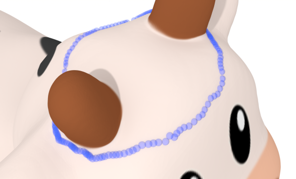
Figure 5: A comparison between a dense uniform sampling, with 281 samples, satisfying the conditions described by Shah et al. [SC13] (on the left) and a non-uniform $\rho$-sampling scheme with only 124 samples (on the right).

Curve properties.

We start from a classical result in differential geometry about the injectivity radius.

Theorem 1 ([Kli95]).

Let $\mathcal{M}$ be a $d$-dimensional Riemannian manifold. For every point $p\in\mathcal{M}$, the restriction of the exponential map $\exp_{p}$ to $\mathcal{B}_{{p},{r}}$ is injective for all $r\leq i_{\mathcal{M}}(p)$ and it is a diffeomorphism onto its image.

From this result, we can deduce that if $r\leq i_{\mathcal{M}}(p)$, then there exists a diffeomorphism between the $r$-ball $\mathcal{B}_{{p},{r}}$ centered at $p$ and the Euclidean $d$-dimensional ball $\mathbb{B}^{d}$, as we can see in the example depicted in Figure 6. We can thus generalize the following important result that holds in 2D:

Lemma 1 ([ABE98]).

Let $\mathcal{C}\subset\mathbb{R}^{2}$ be a closed curve in the plane. For every point $p\in\mathbb{R}^{2}$ and every $r\in\mathbb{R}^{+}$, if the Euclidean disk $D$ of radius $r$ and centered at $p$ contains at least two points of $\mathcal{C}$, then either $D\cap\mathcal{C}$ is a topological 1-disk, or $D$ contains a point of $\Gamma(\mathcal{C})$, or both.

For Riemannian manifolds of arbitrary dimensions we get:

Lemma 2.

Let $\mathcal{C}\subset\mathcal{M}$ be a closed curve on the manifold $\mathcal{M}$. For every point $p\in\mathcal{M}$ and every positive real value $r\leq i_{\mathcal{M}}(p)$, if the $r$-ball $\mathcal{B}_{{p},{r}}$ centered at $p$ contains at least two points of $\mathcal{C}$, then then either $\mathcal{B}_{{p},{r}}\cap\mathcal{C}$ is a topological 1-disk, or $\mathcal{B}_{{p},{r}}$ contains a point of $\Gamma(\mathcal{C})$, or both.

Corollary 1.

For every point $p\in\mathcal{C}$, and for $r\leq\mathrm{ilfs}({p})$, the ball $\mathcal{B}_{{p},{r}}$ intersects $\mathcal{C}$ in a topological 1-disk.

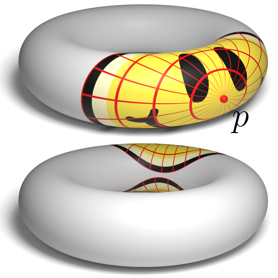
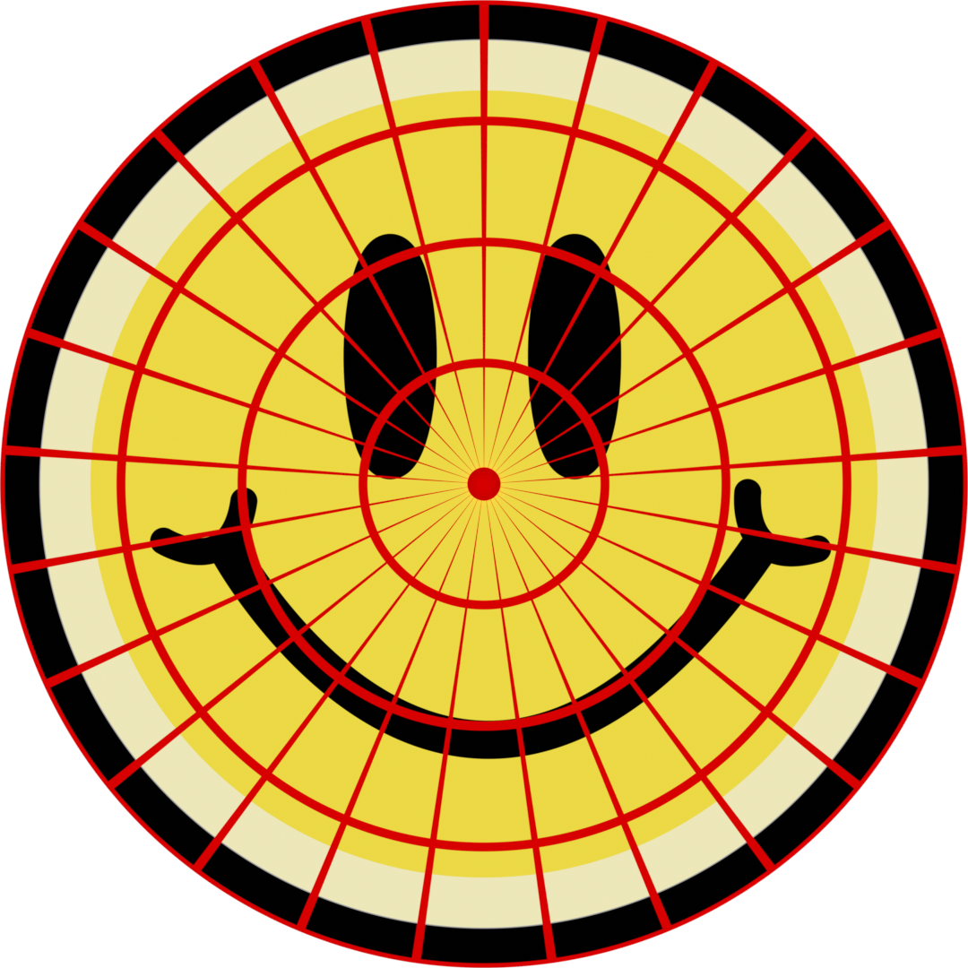
Figure 6: Mapping of an $r$-ball around a point $p$ on a surface (left) to the Euclidean disk $\mathbb{B}^{2}$ (right). The mapping is possible because $r\leq i_{\mathcal{M}}(p)$.

Properties of the sampling.

From 2 and 1, we can infer information on how the samples are distributed.

Proposition 1.

Let $S\subset\mathcal{C}$ be a sampling of the curve. For every point $p\in\mathcal{C}$, let $s_{0},s_{1}\in S$ be the samples such that the interval $I=(s_{0},s_{1})$ is the smallest open interval between samples that contains $p$. If there exists a point $q\in\mathcal{C}$ not belonging to the closure of $I$ that is closer to $p$ than both $s_{0}$ and $s_{1}$ are to $p$, then $d_{\mathcal{M}}(p,q)\geq\mathrm{ilfs}({p})$.

Note that the statement of 1 does not require that $p\notin S$. Indeed, if $p$ is a sample, the two samples that define the smallest interval containing $p$ are its adjacent samples. This is the reason we use the open interval containing $p$, and not the closed version. Given the proper constraints of $\rho$, we can provide additional guarantees.

Corollary 2.

Let $S\subset\mathcal{C}$ be a sampling of the curve, and $s_{0},s_{1}\in S$ be two adjacent samples defining an interval $I=[s_{0},s_{1}]\subset\mathcal{C}$. If $S$ is a $\rho$-sampling with $\rho<1$, then for every point $p\in I$, the closest sample to $p$ is either $s_{0}$ or $s_{1}$.

Proposition 2.

Let $S\subset\mathcal{C}$ be a $\rho$-sampling, with $\rho<1$. For any two consecutive samples $s_{0},s_{1}$, let $I=[s_{0},s_{1}]$ be the interval between them. Then we have $d_{\mathcal{M}}(s_{0},s_{1})<2\mathrm{ireach}({I})$.

4.2 SIGDV graph on manifolds

In their work for 2D curve reconstruction, Marin et al. [MOW22] introduced the SIGDT proximity graph, obtained by intersecting the Delaunay triangulation with the Spheres-of-Influence graph.

Definition 11 ([Tou88]).

Given a set of vertices $V=\{v_{1},\cdots,v_{n}\}\subset\mathcal{M}$, the Spheres-of-Influence (SIG) graph of $V$ is a graph $G=(V,E)$ such that two nodes are connected if and only if they are closer than the sum of distances to their respective nearest neighbors. Namely

$$e=\{v_{i},\ v_{j}\}\in E\iff d_{\mathcal{M}}(v_{i},v_{j})\leq\delta_{NN}(v_{i})+\delta_{NN}(v_{j})\,,$$ (11)

where $\delta_{NN}(v_{i})=\min_{j\neq i}d_{\mathcal{M}}(v_{i},v_{j})$ is the distance of $v_{i}$ from its nearest neighbor.

The SIGDT is proved, in the planar setting, to contain the correct reconstruction of the curve under $\rho$-sampling conditions with $\rho<1$ and non-uniformity ratio $u<2$, and being a subgraph of the Delaunay triangulation, it is also a sparse graph. These conditions make it a good starting point for finding the reconstruction of the curve. We provide an example of the construction of the SIGDT in Figure 7.

Figure 7: For a set of points in 2D, the intersection between Delaunay triangulation (red) and SIG (blue) creates the SIGDT (yellow). The edges removed from Delaunay triangulation and SIG are shown with dashed lines of the graphs’ corresponding colors.

While the Spheres-of-Influence graph is only defined in terms of distances, lifting the Delaunay triangulation to manifold domains is less intuitive. The lack of a coordinate system makes it difficult to generalize classical construction algorithms like the Bowyer-Watson method [Bow81, Wat81] to non-Euclidean metric spaces. However, we use the dual graph of the Delaunay triangulation – the Voronoi partitioning, which is defined only in terms of distances [AKL13]. This duality has already been exploited for lifting the Delaunay triangulation to surfaces and has proved to maintain many properties of the 2D triangulation, such as providing angle stability and containing the nearest neighbor graph [Wan15, LFXH17]. Furthermore, it can be shown that computing the Voronoi partitioning of discrete manifolds is an efficient operation that can be achieved in time $\mathcal{O}\left({|V|\log|V|\log k}\right)$, being $|V|$ the number of vertices and $k$ the number of samples [PC06, MBRM24].

Differently from the Euclidean space, the dual of a Voronoi decomposition does not always guarantee a valid triangulation of the point set, as there are some additional constraints that the samples must satisfy [ACDL00, DZM07]. If these are not satisfied, the dual still forms a sparse graph that encodes the proximity of samples well. In order to obtain the dual of the Voronoi, we connect samples that generate adjacent partitions, as shown in Figure 8. By removing all the edges from the Voronoi dual that do not also satisfy 11, we obtain the intersection between the Spheres-of-Influence graph and the dual Voronoi graph, which we denote as SIGDV, and which provides a generalization for the SIGDT graph.

The following statements about our graph hold. Proofs are provided in Appendix A.

Lemma 3.

Let $s_{0},s_{1}\in\mathcal{C}$ be consecutive samples from a $\rho$-sampling $S\in C$, with $\rho<1$. The edge $e(s_{0},s_{1})$ belongs to the dual Voronoi graph of $S$.

Lemma 4.

Let $s_{0},s_{1},s_{2},s_{3}\in\mathcal{C}$ be consecutive samples from a $\rho,u$-sampling $S\in C$, with $\rho<1$ and $u<2$. The edge $e(s_{1},s_{2})$ belongs to the Spheres-of-Influence graph of $S$.

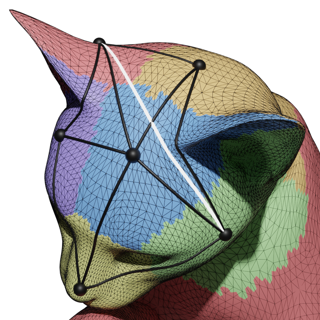
Figure 8: Left: a triangular mesh with some surface samples. Center: the geodesic Voronoi partitioning induced by the samples on the mesh, and its dual graph (white) obtained by locating the shortest geodesic paths between samples in adjacent partitions. Right: the SIGDV (black) obtained by removing the edges not in the SIG.

Finally, we prove (in Appendix A) that SIGDV contains the correct reconstruction under analogous sampling conditions as the 2D case:

Theorem 2.

Let $\mathcal{M}$ be a $d$-dimensional Riemannian manifold, possibly with boundary $\partial\mathcal{M}$, and equipped with a geodesic distance $d_{\mathcal{M}}:\mathcal{M}\times\mathcal{M}\to\mathbb{R}$. Let $\mathcal{C}\subset\mathcal{M}$ be a curve on the manifold $\mathcal{M}$, and $S=\{s_{1},\cdots,s_{k}\}\subset\mathcal{C}$ be a $\rho,u$-sampling of $\mathcal{C}$, with $\rho<1$ and $u<2$. The edge connecting any pair of consecutive samples is part of the SIGDV of $S$.

4.3 Curve reconstruction as a Traveling Salesman Problem

While 2 guarantees that SIGDV contains the correct reconstruction, it may contain additional edges. This problem was also addressed by Marin et al. [MOW22] for their SIGDT planar curve reconstruction algorithm. In their pipeline, the authors propose to apply a series of inflating and sculpting operations until they obtain a manifold curve. In our case, this is not applicable, as in non-Euclidean spaces, such as manifolds, it is not always possible to define the notions of “inside” and “outside” of a curve.

To overcome this issue, we note that the edges of the correct reconstruction should create a cycle such that each sample is visited only once. Various ways of extracting these edges exist in the literature, such as the identification of a Hamiltonian cycle [IN07, Bjo14] or the solution to a Traveling Salesman Problem (TSP). We choose to use a variant of TSP in our experiments, as in the planar case it proves to be a good heuristic for identifying the correct reconstruction [AM00, OPP^∗21].

The Traveling Salesman Problem is a fundamental problem in computer science, and it is at the very core of many optimization problems. Given a set of points, TSP requires finding the shortest path that connects all the points, thus solving the problem of curve reconstruction as well. The problem can be formulated in different spaces and with different connectivity constraints, but all of them have been shown to be NP-hard [Kar75]. However, the importance of the TSP led many researchers to deploy approximated solutions, especially relying on a nearest-neighbor approach [JM97, RBP07] – even though these solutions tend to have a large approximation factor. Other techniques [DMC96, SM15] proved to be much more effective, while paying a small price on time efficiency.

Most of the research related to the TSP assumes complete graphs (i.e., each node is connected to every other node). While we can accept solutions containing edges not belonging to SIGDV, we know that this graph contains the correct reconstruction under some sampling conditions, and hence we want to bias the algorithm to use SIGDV edges, while at the same time guaranteeing an efficient solution.

We start from a solution that exploits the Minimum Spanning Tree of a graph to produce a 2-optimal approximation to the problem (i.e., a solution that is at most two times as expensive as the optimal one) [CLRS22]. Our method is summarized in Algorithm 1, where the input graph $G$ is the SIGDV graph and the matrix $\mathbf{D}$ contains in the entry $\mathbf{D}_{ij}$ the geodesic distance $d_{\mathcal{M}}(i,j)$ between the $i$-th and the $j$-th samples.

Algorithm 1 Algorithm for solving the TSP biased towards SIGDV edges.

1:procedure TSPSolver($G=(V,E)$, $\mathbf{D}\in\mathbb{R}^{|V|\times|V|}$)

2:     $T\leftarrow$ minimum spanning tree of $G$ w.r.t. $\mathbf{D}$

3:     $P\leftarrow$ ordering of $V$ following a pre-order DFS visit of $T$

4:     repeat

5:         Find $(i,j),(\ell,h)\in P$ s.t. $\mathbf{D}_{ij}+\mathbf{D}_{\ell h}>\mathbf{D}_{i\ell}+\mathbf{D}_{jh}$

6:         $P\leftarrow P\setminus\{(i,j),(\ell,h)\}$

7:         $P\leftarrow P\cup\{(i,\ell),(j,h)\}$

8:     until $P$ is unchanged

9:     return $P$

10:end procedure

We first compute the minimum spanning tree $T$ of the graph $G$ and via a pre-ordered Depth-First Search (DFS) visit of $T$ we find an ordering of the nodes in $V$ that we use to build an initial cycle $P$ (Lines 1-2). Since the metric $d_{\mathcal{M}}$ respect the triangular inequality, the cycle $P$ is guaranteed to be a 2-optimal approximation of the TSP [CLRS22]. However, $P$ does not offer any guarantee for the cycle to be a local minimum of the problem. Thus, we post-process the ordering by searching for any pair of edges $(i,j),(\ell,h)$ such that if we swap them into $(i,\ell),(j,h)$ we obtain a shorter cycle, and we iterate this process until no new pair of edges is found (Lines 4-8).

Relaxed sampling conditions.

The sampling conditions imposed by 2 allow for a sparser sampling compared to the state-of-the-art. However, when these conditions are not met, we do not have the guarantee that SIGDV contains the correct reconstruction or any other Hamiltonian cycle. Intersecting the dual Voronoi graph with the SIG could even produce a graph with multiple disconnected components. In some applications (see Reconstructing Curves from Sparse Samples on Riemannian Manifolds) this can be a desired feature, as the clustering can be used to identify multiple curves. When this is not the case and there is only a single curve to reconstruct, we alter the graph to produce a single connected component. First, we build the complete graph $\mathfrak{G}=(\mathfrak{V},\mathfrak{E})$ of the connected components, where each node $N_{i}\in\mathfrak{V}$ represents a single component of SIGDV, and the length of the edge $(N_{i},N_{j})\in\mathfrak{E}$ is given by $\min_{u\in N_{i},v\in N_{j}}d_{\mathcal{M}}(u,v)$. Then, we compute the minimum spanning tree $\mathfrak{T}$ of this graph. For every edge $(N_{i},N_{j})\in\mathfrak{T}$, we add to SIGDV the edge $(u^{*},v^{*})=\operatorname*{arg\,min}_{u\in N_{i},v\in N_{j}}d_{\mathcal{M}}(u,v)$. This pre-processing guarantees that we obtain a single connected component, while, at the same time, adding non-SIGDV edges with minimum total edge length. The choice between single and multiple curve reconstruction is left to the user for full flexibility.

5 Applications

We investigate several diverse applications of our method. We first compare it to the approach proposed by Shah et al. [SC13] (MST) for motion tracking applications, where we show that we are able to reconstruct complex paths with far fewer samples. We show how our method can be applied in processing archaeological data, and how it can improve contour matching results, and we discuss the applicability of our solution to isoline extraction from sparse samples for scientific visualization.

Our method has been implemented in C++, using Eigen [GJ^∗10] and Geometry Central [SC^∗19]. For computing Voronoi diagrams in high-dimensional spaces we use Qhull [BDH96], and for computing the geodesic paths used in our visualizations we use the Flip Geodesics algorithm [SC20].

5.1 Motion tracking

In their work about curve reconstruction on Riemannian manifolds, Shah et al. [SC13] propose, as an application, the reconstruction of curves in the space of rigid motions $SE({3})$ for tracking the motion of an object from position and rotation samples. To apply our method to this task, we first need to define how to compute a Voronoi diagram in $SE({3})$.

As discussed by González-López et al. [GLR95], the group $SE({3})$ can be expressed as the product $SO({3})\times\mathbb{R}^{3}$, $SO({3})$ being the group of rotations in 3D space. The authors propose a method for computing the Voronoi decomposition in $SO({3})$ relying on the following result.

Proposition 3 ([GLR95]).

Given a set of rotations $R=\{r_{i}\}_{i=1}^{k}$ in $SO({3})$ and a set of rotation matrices $R^{\prime}=\{\mathbf{R}_{i}\}_{i=1}^{k}$ in $\mathbb{R}^{3\times 3}$ such that $\mathbf{R}_{i}$ represents the rotation of $r_{i}$, the Voronoi decomposition $\mathrm{Vor}(R,d_{SO({3})})$ of $SO({3})$ w.r.t. the rotations $R$ can be obtained as

$$\mathrm{Vor}(R,d_{SO({3})})=\mathrm{Vor}(R^{\prime},d_{\mathbb{R}^{9}})\cap SO({3})\,.$$ (12)

We improve this result for an easier computation of the Voronoi diagram in the group $SO({3})$. The proof is provided in Appendix A.

Proposition 4.

Given a set of rotations $R=\{r_{i}\}_{i=1}^{k}$ in $SO({3})$ and a set of quaternions $Q=\{q_{i}\}_{i=1}^{k}$ in $\mathbb{H}$ such that $q_{i}$ represents the rotation $r_{i}$, then the Voronoi decomposition $\mathrm{Vor}(R,d_{SO({3})})$ of $SO({3})$ w.r.t. the rotations $R$ can be obtained as

$$\mathrm{Vor}(R,d_{SO({3})})=\mathrm{Vor}(Q,d_{\mathbb{R}^{4}})\cap SO({3})\,.$$ (13)

As proven by González-López et al. [GLR95], this result does not generalize to $SE({3})$, and we must only rely on the Voronoi decomposition of the embedding space. However, by reducing the dimensionality of the embedding space of $SO({3})$ from $\mathbb{R}^{9}$ to $\mathbb{R}^{4}$, we also reduce the dimensionality of the embedding space of $SE({3})$ from $\mathbb{R}^{12}$ to $\mathbb{R}^{7}$. Thus, we can use the Voronoi decomposition in $\mathbb{R}^{7}$ as a reasonable approximation of the Voronoi decomposition in $SE({3})$.

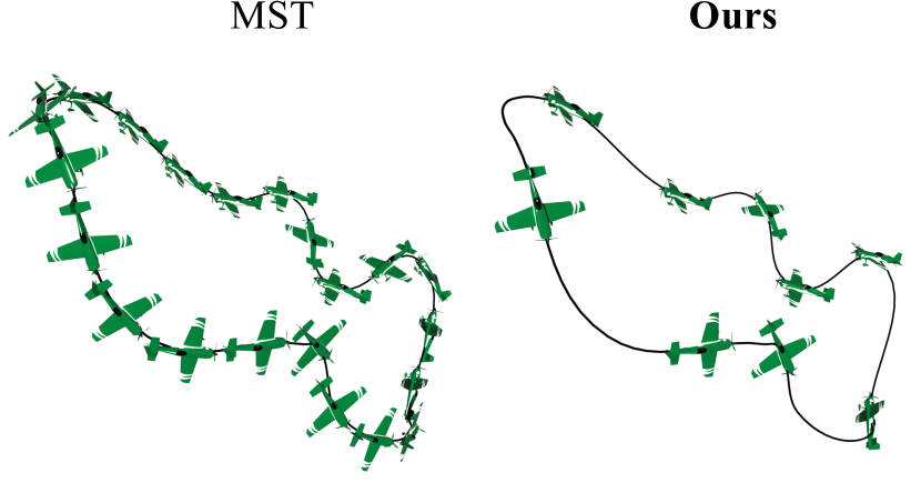
Figure 9: Minimal number of samples for reconstructing the motion of an airplane along a path using MST - left (21), and our approach - right (9). The airplane model has been created by Kemal Çolak and distributed by Sketchfab under the license CC BY 4.0.

In Figure 9 we present an example of motion reconstructed using MST and our solution, and we show the minimum number of samples required by each to obtain a correct reconstruction – 21 for MST and 9 for our method. While our method can deal with sparse non-uniform sampling and still correctly recover the ordering of the samples, it is evident here that MST requires a more dense and uniform sampling scheme. Indeed, the path presents a challenging shape, as the two close turns in the bottom half are very close in space, and the adjacent samples on the curve are very different in terms of rotations. Such curves can be adversarial for MST, as the distance in $SE({3})$ between non-adjacent samples is small, preventing their method from finding a closed curve.

5.2 Virtual cultural heritage

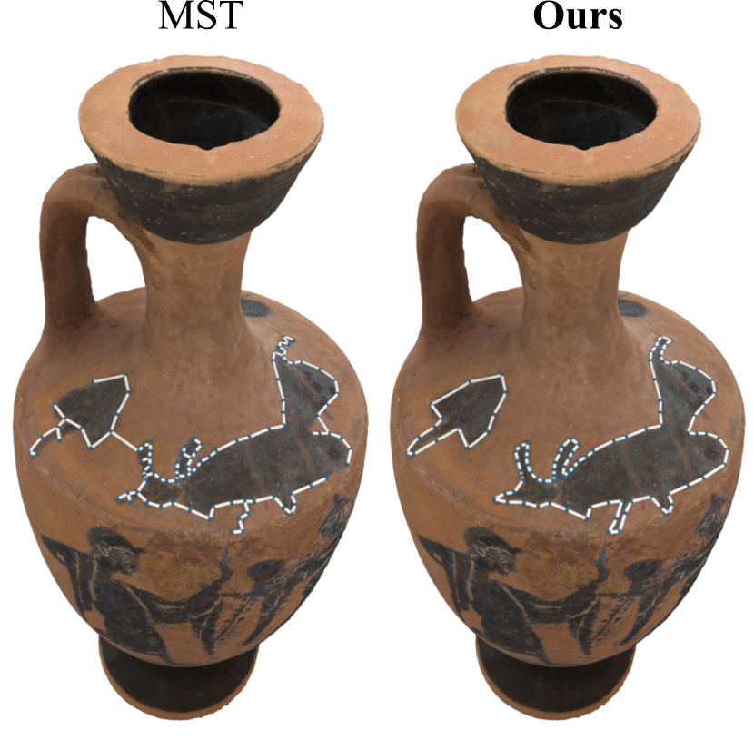
Figure 10: Reconstruction of complex curves (white) on the surface of a clay vase from a set of manually chosen samples (blue). The MST algorithm (left) fails to reconstruct meaningful contours, while ours (right) correctly identifies the two shapes. The vase model has been created by Laura Shea and distributed by Sketchfab under the license CC BY-NC-SA 4.0 DEED.

Scientific visualization and 3D shape analysis are already prevalent in archaeological applications as instruments for handling the always-increasing amount of data available to cultural heritage research [Tal14].

Successful applications of computational geometry to the analysis of archaeological data include the identification of demarcating curves on low reliefs, statues, and other various kinds of cultural heritage artifacts [GTSK13, TBF16], curve matching tasks in 2D and 3D for solving the problem of fragment reconstruction [MK03] and pattern extraction of culturally significant patterns [YP20].

The problem of reconstructing curves on surfaces is closely related to these applications, as there can be cases where missing information from lost pieces could be inferred by knowing the structure of the underlying artifact (e.g. partial designs on vases that could be reconstructed from still existing pieces). In Figure 10 we show that our method can faithfully reconstruct complex shapes on the surface of a vase, precisely contouring the black drawings from a sparse sampling. We also compare our result against the MST algorithm, which is unable to find a closed shape due to the presence of multiple connected components and the large distance among some of the samples.

5.3 Contour matching

Contour matching is a novel task in computer graphics and vision applications that has recently achieved high attention [LRS^∗16, RLB23]. The problem this field is concerned with is how to meaningfully relate a surface to the curve defining its contour, even under non-rigid deformation of the surface [WSSC11].

While the existing approaches reliably compute non-rigid correspondences between shapes and their contour, the task is still new and even state-of-the-art methods do not always provide high-quality guarantees, producing self-intersecting and locally degenerate curves. We show that our curve reconstruction technique can be exploited as a refinement step to improve the contour quality.

For our evaluation, we use the method proposed by Lähner et al. [LRS^∗16] (Elastic2D3D), selecting some instances from the dataset that the authors derive from the FAUST shape collection [BRLB14] where the method produces many degeneracies. From the curve obtained with Elastic2D3D, we randomly extract 3% of the vertices, and we run our algorithm for reconstructing the contour over the target shape.

Figure 11: Examples of how our curve reconstruction method is applied to refine a contour. Given a contour obtained with Elastic2D3D [LRS^∗16], we sample it sparsely and reconnect the samples using the ordering of the contour, MST, and our algorithm.

Even if Elastic2D3D may produce self-intersections and locally degenerate curves, it captures the overall shape of the contour. Thus, a sparse sampling of the curve should give a good sparse contour. As shown in the examples from Figure 11, with our algorithm we can smooth the results of Elastic2D3D, resolving the self-intersections and producing non-degenerate curves. For reference, we also connect the samples with their original ordering, proving that our method’s reordering of the samples improves the overall result.

MST cannot produce a valid closed curve in any of the tested cases, as the conditions imposed by the algorithm require the sampling to be denser and more uniform for the minimum spanning tree to result in a chain. This is primarily due to the presence of degeneracies in the curve produced by Elastic2D3D in the form of jagged edges. Hence, two points sampled from a degenerate section of the curve would very likely result in a branch on the minimum spanning tree. We validate this argument by running the MST algorithm on different sampling densities spanning from 1% to 100% of the curve vertices produced by Elastic2D3D, and the minimum spanning tree never results in a chain.

5.4 Sparse data visualization

Having shown that our method can improve contours already computed by reordering a sparse set of their samples, we now move onto another definition of contours, namely their existence as isolines (i.e., lines connecting data points with the same value). We show how our method can be used to visualize large data by only using a sparse subset of it.

Analyzing large datasets and being able to extract meaningful visual information is a challenge for various scientific visualization fields. We choose to focus on meteorological data in this application, and considering the increase in computational power and available tools, the information we can obtain has increased exponentially. Methods to quickly process massive amounts of data are required, to allow scientists to interpret and extract the most relevant information. One method to deal with very dense data is to choose a subset, that acts as an overview, and then use this global view of data to find and focus on a specific area of interest at a higher resolution [KW19, MHS^∗20]. This facilitates a quicker understanding of the data at different levels while using less data and hence, less computational power.

In the field of visualizing meteorological data, an important problem arises from the numerical issues of projecting information that exists on the Earth’s surface onto a plane, where at least one of the following properties has to be sacrificed: distances, angles, or areas. We bypass this challenge by working with samples directly on surfaces and allowing for a three-dimensional interaction and visualization of data. A common way of visualizing various properties of meteorological data is presented by contour lines (or isolines) where data points with equal or similar (up to a threshold) values are connected to represent all the possible points that have similar data [RBS^∗17].

Meteorological datasets, such as the ones provided by the European Centre for Medium-Range Weather Forecasts [ecm], contain massive amounts of data for every recorded timestep, at a resolution of 0.25 degrees in both latitude and longitude, with up to 90 parameters such as temperature, humidity, pressure. Analyzing the entirety of the data at a global level is a tedious and complex task, and we propose to combine the deformation-free surface representation with a sparse sampling of the dataset to reconstruct contours for an easier understanding of global information.

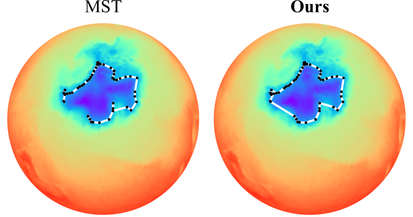
Figure 12: Samples (black) with approximately the same temperatures connected using the MST algorithm (left) and our method (right) to form a contour line (white) for a region with a temperature of 230$\pm$0.3K on the globe, for a single timestep.

In Figure 12, we use the global temperature values recorded on 31${}^{\text{st}}$ of March 2024, at midnight, and use a subset of the values (a quarter of the initial array, by skipping every second and fourth row) to minimize the amount of data. The texture of the mesh represents the ground truth temperatures. We then extract the points with a temperature of 230$\pm$0.3K and connect them to obtain the corresponding contour line, only requiring 63 samples to reconstruct the isoline. In contrast, the MST algorithm is unable to reconstruct the curve due to the non-uniformity of the samples. The data we used is based on data and products of the European Centre for Medium-Range Weather Forecasts (ECMWF), under CC BY 4.0. license.

6 Conclusions

We have generalized the sampling requirements of closed curves from the Euclidean plane $\mathbb{R}^{2}$ to Riemannian manifold domains of arbitrary dimension. By taking inspiration from the literature on planar curve reconstruction, we designed a new method for recovering the original connectivity from a sparse sampling by biasing an instance of the traveling salesman problem with a coarse graph, which exhibits strong theoretical guarantees. We have proved the effectiveness of our method by testing it in different scenarios and various applications involving real-world data, showing that it outperforms the existing previous solution and that it provides a correct result, while in many cases the state-of-the-art method fails.

As for future directions, we intend to explore possible relaxations of the starting graph to offer stronger theoretical guarantees even under adversarial samplings. Furthermore, we notice that when the sampling conditions satisfy our constraints, the original reconstruction forms a Hamiltonian cycle inside the SIGDV graph, and thus more sophisticated techniques for identifying such a cycle could be worth future investigation. Another possible avenue of future development is dealing with more general classes of curves, as these could provide an important tool in pattern extraction, where not all elements are closed smooth curves. Finally, as the reconstruction of curves in non-Euclidean domains is a barely explored topic, we identify the absence of a unified validation benchmark for quantitative analyses and we intend to fill this gap in the future.

Appendix A Proofs

In this appendix, we provide the proofs of all our claims.

Lemma 2.

Let $\mathcal{C}\subset\mathcal{M}$ be a closed curve on the manifold $\mathcal{M}$. For every point $p\in\mathcal{M}$ and every positive real value $r\leq i_{\mathcal{M}}(p)$, if the $r$-ball $\mathcal{B}_{{p},{r}}$ centered at $p$ contains at least two points of $\mathcal{C}$, then then either $\mathcal{B}_{{p},{r}}\cap\mathcal{C}$ is a topological 1-disk, or $\mathcal{B}_{{p},{r}}$ contains a point of $\Gamma(\mathcal{C})$, or both.

Proof.

Let us denote $\mathcal{F}=\mathcal{B}_{{p},{r}}\cap\mathcal{C}$, and let be $d$ the dimensionality of the manifold $\mathcal{M}$.

First, let $d=2$. Since $r\leq i_{\mathcal{M}}(p)$, then by 1 we can define a diffeomorphism $\varphi:\mathcal{B}_{{p},{r}}\to\mathbb{B}^{2}$. Since $\mathcal{F}\subset\mathcal{B}_{{p},{r}}$, then $\varphi(\mathcal{F})\subset\mathbb{B}^{2}$, and by 1 either $\varphi(\mathcal{F})$ is a topological 1-disk or $\mathbb{B}^{2}$ contains a point of its medial axis. Since $\varphi$ is a diffeomorphism, either $\mathcal{F}$ is a topological 1-disk or $\mathcal{B}_{{p},{r}}$ contains a point of its medial axis.

For general $d$, we again define a diffeomorphism $\varphi:\mathcal{B}_{{p},{r}}\to\mathbb{B}^{d}$. Since $\mathbb{B}^{d}$ is a $d$-dimensional Euclidean space ($d>2$), we can build a 2-dimensional manifold $\mathcal{M}^{\prime}$ embedded in $\mathbb{B}^{d}$ such that:

• $\mathcal{M}^{\prime}$ is a topological 2-dimensional disk and contains no holes;

• the boundary of $\mathcal{M}^{\prime}$ entirely belongs to the boundary of $\mathbb{B}^{d}$;

• $\mathcal{M}^{\prime}$ contains both $p$ and $\varphi(\mathcal{F})$;

• $p$ is equidistant from the boundary of $\mathcal{M}^{\prime}$ and has distance $r^{\prime}$ from it.

$\mathcal{M}^{\prime}$ is a 2-dimensional $r^{\prime}$-ball centered at $p$ which intersects the curve $\mathcal{C}$ in $\varphi(\mathcal{F})$, and we have already proved that this either means $\varphi(\mathcal{F})$ is a topological 1-disk or $\mathcal{M}^{\prime}$ contains a point of the medial axis. Since $\mathcal{M}^{\prime}\subset\mathbb{B}^{d}$ and $\varphi^{-1}(\mathcal{M}^{\prime})\subset\mathcal{B}_{{p},{r}}$, and since $\varphi$ is a diffeomorphism, the claim follows. ∎

Corollary 1.

For every point $p\in\mathcal{C}$, and for $r\leq\mathrm{ilfs}({p})$, the ball $\mathcal{B}_{{p},{r}}$ intersects $\mathcal{C}$ in a topological 1-disk.

Proof.

Let $\mathcal{B}_{{p},{r}}$ be a $r$-ball centered at $p$, for some $r\in\mathbb{R}^{+}$, that does not intersect $\mathcal{C}$ in a topological 1-disk. If that is the case, then either $r>i_{\mathcal{M}}>\mathrm{ilfs}({p})$ or $\mathcal{B}_{{p},{r}}$ contains at least one point $m$ of the medial axis (by 2). This would lead to $r>d_{\mathcal{M}}(p,m)>\mathrm{lfs}({p})>\mathrm{ilfs}({p})$.

∎

Proposition 1.

Let $S\subset\mathcal{C}$ be a sampling of the curve. For every point $p\in\mathcal{C}$, let $s_{0},s_{1}\in S$ be the samples such that the interval $I=(s_{0},s_{1})$ is the smallest open interval between samples that contains $p$. If there exists a point $q\in\mathcal{C}$ not belonging the the closure of $I$ that is closer to $p$ than both $s_{0}$ and $s_{1}$ are to $p$, then $d_{\mathcal{M}}(p,q)\geq\mathrm{ilfs}({p})$.

Proof.

Let us denote $\delta=d_{\mathcal{M}}(p,q)$, and consider the $r$-ball $\mathcal{B}_{{p},{\delta}}$ of size $\delta$ and centered at $p$.

Since $s_{0}$ and $s_{1}$ lie outside $\mathcal{B}_{{p},{\delta}}$, $p$ lies inside $\mathcal{B}_{{p},{\delta}}$, and $\mathcal{B}_{{p},{\delta}}$ touches $q$, then either the intersection $\mathcal{F}=\mathcal{C}\cap\mathcal{B}_{{p},{\delta}}$ has two connected components, or $\mathcal{C}$ is tangent to $\mathcal{B}_{{p},{\delta}}$ at $q$.

If $\mathcal{F}$ has two connected components, then by 1 $\delta>\mathrm{ilfs}({p})$.

If $\mathcal{C}$ is is tangent to $\mathcal{B}_{{p},{\delta}}$ at $q$, then for every $\varepsilon>0$, the ball $\mathcal{B}_{{p},{\delta+\varepsilon}}$ would intersect $\mathcal{C}$ in two connected components, meaning $\delta+\varepsilon>\mathrm{ilfs}({p})$. Hence, $\delta\geq\mathrm{ilfs}({p})$. ∎

Corollary 2.

Let $S\subset\mathcal{C}$ be a sampling of the curve, and $s_{0},s_{1}\in S$ be two adjacent samples defining an interval $I=[s_{0},s_{1}]\subset\mathcal{C}$. If $S$ is a $\rho$-sampling with $\rho<1$, then for every point $p\in I$, the closest sample to $p$ is either $s_{0}$ or $s_{1}$.

Proof.

Assume the closest sample to $p$ is some $s_{i}\neq s_{0},s_{1}$, and let us denote $\delta=\min(d_{\mathcal{M}}(p,s_{0}),d_{\mathcal{M}}(p,s_{1}))$. Then $\delta>d_{\mathcal{M}}(p,s_{i})\geq\mathrm{ilfs}({p})\geq\mathrm{ireach}({I})$. But by definition of $\rho$-sampling, $\delta<\rho\mathrm{ireach}({I})$, which contradicts $\delta>\mathrm{ireach}({I})$ for $\rho<1$. ∎

Proposition 2.

Let $S\subset\mathcal{C}$ be a $\rho$-sampling, with $\rho<1$. For any two consecutive samples $s_{0},s_{1}$, let $I=[s_{0},s_{1}]$ be the interval between them. Then we have $d_{\mathcal{M}}(s_{0},s_{1})<2\mathrm{ireach}({I})$.

Proof.

Consider a point $p$ in the interval $I=[s_{0},s_{1}]$ such that $d_{\mathcal{M}}(s_{0},p)=d_{\mathcal{M}}(s_{1},p)$. That point must be at $d\geq\frac{1}{2}d_{\mathcal{M}}(s_{0},s_{1})$ from $s_{0}$, and by definition of $\rho$-sampling with $\rho<1$, $d<\mathrm{ireach}({I})\leq\mathrm{ilfs}({p})$. By 2, the closest samples to $p$ must be $s_{0}$ and $s_{1}$, and we have $d_{\mathcal{M}}(s_{0},s_{1})\leq 2d<2\ \mathrm{ireach}({I})$. ∎

Lemma 3.

Let $s_{0},s_{1}\in\mathcal{C}$ be consecutive samples from a $\rho$-sampling $S\in C$, with $\rho<1$. The edge $e(s_{0},s_{1})$ belongs to the dual Voronoi graph of $S$.

Proof.

Let $I=[s_{0},s_{1}]\subset\mathcal{C}$ be the interval of $\mathcal{C}$ connecting samples $s_{0}$ and $s_{1}$, and let $p\in I$ be a point such that $d_{\mathcal{M}}(s_{0},p)=d_{\mathcal{M}}(s_{1},p)$. We consider the $r$-ball $\mathcal{B}_{{p},{r}}$ centered at $p$, where $r=d_{\mathcal{M}}(p,s_{i})$ is the distance from $p$ to its closest sample $s_{i}$.

By 2, $s_{i}$ must be either $s_{0}$ or $s_{1}$, yielding $r=d_{\mathcal{M}}(s_{0},p)=d_{\mathcal{M}}(s_{1},p)$. Then the boundary between the Voronoi cells of $s_{0}$ and $s_{1}$ is not empty (as it contains at least $p$), and the edge $e(s_{0},s_{1})$ is the dual of their shared Voronoi boundary. ∎

Lemma 4.

Let $s_{0},s_{1},s_{2},s_{3}\in\mathcal{C}$ be consecutive samples from a $\rho,u$-sampling $S\in C$, with $\rho<1$ and $u<2$. The edge $e(s_{1},s_{2})$ belongs to the Spheres-of-Influence graph of $S$.

Proof.

We split the proof into four cases.

Case 1: If $s_{1}$ is the nearest neighbor of $s_{2}$, or vice versa, then the edge $e$ trivially belongs to SIG.

Case 2: If $s_{0},s_{3}$ are the nearest neighbors of $s_{1}$ and $s_{2}$ respectively, the non-uniformity ratio $u<2$ imposes $d_{\mathcal{M}}(s_{0},s_{1}),d_{\mathcal{M}}(s_{2},s_{3})>\frac{1}{2}d_{\mathcal{M}}(s_{1},s_{2})$, meaning that $d_{\mathcal{M}}(s_{0},s_{1})+d_{\mathcal{M}}(s_{2},s_{3})>d_{\mathcal{M}}(s_{1},s_{2})$. Then the edge $e$ belongs to SIG by definition.

Case 3: Now, suppose neither $s_{0}$ nor $s_{2}$ is a nearest neighbor for $s_{1}$, but $s_{3}$ is a nearest neighbor for $s_{2}$. Then, the distance from $s_{2}$ to its nearest neighbor is $d_{2}=d_{\mathcal{M}}(s_{2},s_{3})$, and let $d_{1}=d_{\mathcal{M}}(s_{1},s_{i})$ be the distance from $s_{1}$ to its nearest neighbor $s_{i}$. If $d_{1}+d_{2}\geq d_{\mathcal{M}}(s_{1},s_{2})$, the edge belongs to SIG by definition.

Otherwise, we must have $d_{1}<d_{\mathcal{M}}(s_{1},s_{2})-d_{2}$. Because of the non-uniformity ratio $u<2$, we know that $\frac{1}{2}d_{\mathcal{M}}(s_{1},s_{2})<d_{2}<2d_{\mathcal{M}}(s_{1},s_{2})$, and hence $d_{1}<\frac{1}{2}d_{\mathcal{M}}(s_{1},s_{2})$. By 2, $d_{1}<\mathrm{ireach}({[s_{1},s_{2}]})\leq\mathrm{ilfs}({s_{1}})$. However, since $s_{i}$ is not adjacent to $s_{1}$, by 1 we have $d_{1}\geq\mathrm{ilfs}({s_{1}})$, which contradicts the above $d_{1}<\mathrm{ilfs}({s_{1}})$.

Case 4: Finally, suppose neither $s_{0}$ nor $s_{2}$ is a nearest neighbor for $s_{1}$, and neither $s_{1}$ nor $s_{3}$ is a nearest neighbor for $s_{2}$. If that is the case, a sample $s_{i}$ must lie at distance $d_{1}=d_{\mathcal{M}}(s_{i},s_{1})$, and 1 requires $d_{1}\geq\mathrm{ilfs}({s_{1}})$. We also must have a sample $s_{j}$ lie at distance $d_{2}=d_{\mathcal{M}}(s_{2},s_{j})$ from $s_{2}$, which is the nearest neighbor of $s_{2}$, and 1 requires $d_{2}\geq\mathrm{ilfs}({s_{2}})$. If $d_{1}+d_{2}\geq d_{\mathcal{M}}(s_{1},s_{2})$, then the edge $e$ belongs to SIG by definition. Suppose then $d_{1}+d_{2}<d_{\mathcal{M}}(s_{1},s_{2})$, and let us denote $r_{1,2}=\min(\mathrm{ilfs}({s_{1}}),\mathrm{ilfs}({s_{2}}))$. 2 requires $d_{1}+d_{2}<d_{\mathcal{M}}(s_{1},s_{2})<2r_{1,2}$. Since $d_{1}\geq\mathrm{ilfs}({s_{1}})\geq r_{1,2}$, we have $d_{2}<r_{1,2}$, which contradicts $d_{2}\geq\mathrm{ilfs}({s_{2}})\geq r_{1,2}$. ∎

Theorem 2.

Let $\mathcal{M}$ be a $d$-dimensional Riemannian manifold, possibly with boundary $\partial\mathcal{M}$, and equipped with a geodesic distance $d_{\mathcal{M}}:\mathcal{M}\times\mathcal{M}\to\mathbb{R}$. Let $\mathcal{C}\subset\mathcal{M}$ be a curve on the manifold $\mathcal{M}$, and $S=\{s_{1},\cdots,s_{k}\}\subset\mathcal{C}$ be a $\rho,u$-sampling of $\mathcal{C}$, with $\rho<1$ and $u<2$. The edge connecting any pair of consecutive samples is part of the SIGDV of $S$.

Proof.

By 3 the edge $e$ belongs to the dual Voronoi connectivity, and by 4 the edge $e$ belongs to SIG. Then the edge also belongs to their intersection SIGDV. ∎

Proposition 4.

Given a set of rotations $R=\{r_{i}\}_{i=1}^{k}$ in $SO({3})$ and a set of quaternions $Q=\{q_{i}\}_{i=1}^{k}$ in $\mathbb{H}$ such that $q_{i}$ represents the rotation $r_{i}$, then the Voronoi decomposition $\mathrm{Vor}(R,d_{SO({3})})$ of $SO({3})$ w.r.t. the rotations $R$ can be obtained as

$$\mathrm{Vor}(R,d_{SO({3})})=\mathrm{Vor}(Q,d_{\mathbb{R}^{4}})\cap SO({3})\,.$$ (14)

Proof.

Let $r_{p},r_{q}\in SO({3})$ be two rotations, and let $p=(p_{w},p_{x},p_{y},p_{z}),q=(q_{w},q_{x},q_{y},q_{z})\in\mathbb{H}$ be the two quaternions representing them. Let $q^{*}$ be the conjugate of $q$. We know that the angular distance between $r_{p}$ and $r_{q}$ can be expressed as the angle of rotation of the quaternion $t=(t_{w},t_{x},t_{y},t_{z})=pq^{*}$, which in turn is given by $2\arccos(t_{w})=2\arccos(\langle p,q\rangle)$.

We also know that the squared Euclidean distance between $p$ and $q$ is given by $\|p-q\|^{2}=\|p\|^{2}+\|q\|^{2}-2\langle p,q\rangle$. Since the quaternions express rotations, they have unitary norm, meaning $\|p-q\|^{2}=2-2\langle p,q\rangle$. Thus, the angular distance between $r_{p}$ and $r_{q}$ can be expressed as

$$d_{SO({3})}(r_{p},r_{q})=2\arccos(\langle p,q\rangle)=2\arccos\left(1-\frac{\|p-q\|^{2}}{2}\right)\,.$$

Since $\langle p,q\rangle$ is bounded by $-1$ and $1$ ($\langle p,q\rangle=\|p\|\|q\|\cos(\theta)=\cos(\theta)$, as $p$ and $q$ are unitary), and since $\arccos(\cdot)$ is a decreasing function on $[-1,1]$, then for any rotation $r_{w}\in SO({3})$ and its corresponding quaternion $w\in\mathbb{H}$ we get that $d_{SO({3})}(r_{p},r_{w})<d_{SO({3})}(r_{q},r_{w})\iff\langle p,w\rangle>\langle q,w\rangle$, but we also know that $\langle p,w\rangle>\langle q,w\rangle\iff\|p-w\|^{2}<\|q-w\|^{2}$. Thus, it must be true that

$$d_{SO({3})}(r_{p},r_{w})<d_{SO({3})}(r_{q},r_{w})\quad\iff\quad\|p-w\|<\|q-w\|\,.$$

This proves that the distance functions $d_{SO({3})}$ and $d_{\mathbb{R}{4}}$ preserve the distance relationships between rotations in $SO({3})$, meaning that $\mathrm{Vor}(R,d_{SO({3})})=\mathrm{Vor}(Q,d_{\mathbb{R}^{4}})\cap SO({3})$. ∎

References

- [ABE98] Amenta N., Bern M., Eppstein D.: The crust and the beta-skeleton: Combinatorial curve reconstruction. Graphical Models and Image Processing 60 (01 1998), 125–135.
- [ACDL00] Amenta N., Choi S., Dey T. K., Leekha N.: A simple algorithm for homeomorphic surface reconstruction. In Proceedings of the sixteenth annual symposium on Computational geometry (2000), pp. 213–222.
- [ACK01] Amenta N., Choi S., Kolluri R. K.: The power crust. In Proceedings of the Sixth ACM Symposium on Solid Modeling and Applications (New York, NY, USA, 2001), SMA ’01, Association for Computing Machinery, p. 249–266. URL: https://doi.org/10.1145/376957.376986, doi:10.1145/376957.376986.
- [Ado] Adobe Inc.: Adobe illustrator. URL: https://adobe.com/products/illustrator.
- [AKL13] Aurenhammer F., Klein R., Lee D.: Voronoi Diagrams And Delaunay Triangulations. World Scientific Publishing Company, 2013. URL: https://books.google.it/books?id=cic8DQAAQBAJ.
- [AM00] Althaus E., Mehlhorn K.: Tsp-based curve reconstruction in polynomial time. In Proceedings of the eleventh annual ACM-SIAM symposium on Discrete algorithms (2000), pp. 686–695.
- [BDH96] Barber C. B., Dobkin D. P., Huhdanpaa H.: The quickhull algorithm for convex hulls. ACM Transactions on Mathematical Software (TOMS) 22, 4 (1996), 469–483.
- [Bjo14] Bjorklund A.: Determinant sums for undirected hamiltonicity. SIAM Journal on Computing 43, 1 (2014), 280–299.
- [Blu67] Blum H.: A transformation for extracting new descriptions of shape. Models for the perception of speech and visual form (1967), 362–380.
- [Bow81] Bowyer A.: Computing Dirichlet tessellations*. The Computer Journal 24, 2 (01 1981), 162–166. URL: https://doi.org/10.1093/comjnl/24.2.162, arXiv:https://academic.oup.com/comjnl/article-pdf/24/2/162/967239/240162.pdf, doi:10.1093/comjnl/24.2.162.
- [BRLB14] Bogo F., Romero J., Loper M., Black M. J.: Faust: Dataset and evaluation for 3d mesh registration. In Proceedings of the IEEE conference on computer vision and pattern recognition (2014), pp. 3794–3801.
- [CDGDS13] Crane K., De Goes F., Desbrun M., Schröder P.: Digital geometry processing with discrete exterior calculus. In ACM SIGGRAPH 2013 Courses (2013), pp. 1–126.
- [CLRS22] Cormen T. H., Leiserson C. E., Rivest R. L., Stein C.: Introduction to algorithms. MIT press, 2022.
- [DC16] Do Carmo M. P.: Differential geometry of curves and surfaces: revised and updated second edition. Courier Dover Publications, 2016.
- [DK99] Dey T. K., Kumar P.: A simple provable algorithm for curve reconstruction. In Proceedings of the Tenth Annual ACM-SIAM Symposium on Discrete Algorithms (USA, 1999), SODA ’99, Society for Industrial and Applied Mathematics, p. 893–894.
- [DMC96] Dorigo M., Maniezzo V., Colorni A.: Ant system: optimization by a colony of cooperating agents. IEEE transactions on systems, man, and cybernetics, part b (cybernetics) 26, 1 (1996), 29–41.
- [DW02] Dey T., Wenger R.: Fast reconstruction of curves with sharp corners. Int. J. Comput. Geometry Appl. 12 (10 2002), 353–400. doi:10.1142/S0218195902000931.
- [DZM07] Dyer R., Zhang H., Möller T.: Voronoi-delaunay duality and delaunay meshes. In Proceedings of the 2007 ACM symposium on Solid and physical modeling (2007), pp. 415–420.
- [ecm] European centre for medium-range weather forecasts. http://www.ecmwf.int/.
- [EMP∗03] Ebert D. S., Musgrave F. K., Peachey D., Perlin K., Worley S.: Texturing & modeling: a procedural approach. Morgan Kaufmann, 2003.
- [Fed59] Federer H.: Curvature measures. Transactions of the American Mathematical Society 93, 3 (1959), 418–491.
- [GJ∗10] Guennebaud G., Jacob B., et al.: Eigen. URl: http://eigen. tuxfamily. org 3, 1 (2010).
- [GLR95] González-López M., Recio T.: Voronoi computability in SE(3). 12 1995, pp. 137–148. doi:10.1515/9783110881271.137.
- [GTSK13] Gilboa A., Tal A., Shimshoni I., Kolomenkin M.: Computer-based, automatic recording and illustration of complex archaeological artifacts. Journal of Archaeological Science 40, 2 (2013), 1329–1339.
- [Har01] Hart J. C.: Perlin noise pixel shaders. In Proceedings of the ACM SIGGRAPH/EUROGRAPHICS workshop on Graphics hardware (2001), pp. 87–94.
- [HDD∗92] Hoppe H., Derose T., Duchamp T., Mcdonald J., Stuet-zle W.: Surface reconstruction from unorganized point clouds.
- [HH13] Hall B. C., Hall B. C.: Lie groups, Lie algebras, and representations. Springer, 2013.
- [IN07] Iwama K., Nakashima T.: An improved exact algorithm for cubic graph tsp. In Computing and Combinatorics: 13th Annual International Conference, COCOON 2007, Banff, Canada, July 16-19, 2007. Proceedings 13 (2007), Springer, pp. 108–117.
- [Ink] Inkscape Project: Inkscape. URL: https://inkscape.org.
- [JM97] Johnson D. S., McGeoch L. A.: The traveling salesman problem: A case study in local optimization. Local search in combinatorial optimization 1, 1 (1997), 215–310.
- [Kar75] Karp R. M.: On the computational complexity of combinatorial problems. Networks 5, 1 (1975), 45–68.
- [KBH06] Kazhdan M., Bolitho M., Hoppe H.: Poisson Surface Reconstruction. In Symposium on Geometry Processing (2006), Sheffer A., Polthier K., (Eds.), The Eurographics Association. doi:10.2312/SGP/SGP06/061-070.
- [Kli95] Klingenberg W.: Riemannian geometry, vol. 1. Walter de Gruyter, 1995.
- [KST08] Kolomenkin M., Shimshoni I., Tal A.: Demarcating curves for shape illustration. In ACM SIGGRAPH Asia 2008 papers. 2008, pp. 1–9.
- [KW19] Kim J. K., Wang Z.: Sampling techniques for big data analysis. International Statistical Review 87 (2019), S177–S191.
- [LFXH17] Liu Y.-J., Fan D., Xu C.-X., He Y.: Constructing intrinsic delaunay triangulations from the dual of geodesic voronoi diagrams. ACM Trans. Graph. 36, 2 (apr 2017). URL: https://doi.org/10.1145/2999532, doi:10.1145/2999532.
- [LRS∗16] Lahner Z., Rodola E., Schmidt F. R., Bronstein M. M., Cremers D.: Efficient globally optimal 2d-to-3d deformable shape matching. In Proceedings of the IEEE Conference on Computer Vision and Pattern Recognition (2016), pp. 2185–2193.
- [MBMR22] Maggioli F., Baieri D., Melzi S., Rodolà E.: Newton’s fractals on surfaces via bicomplex algebra. In ACM SIGGRAPH 2022 Posters. 2022, pp. 1–2.
- [MBRM24] Maggioli F., Baieri D., Rodolà E., Melzi S.: Rematching: Low-resolution representations for scalable shape correspondence, 2024. arXiv:2305.09274.
- [MG23] Mishra S., Granskog J.: CLIP-based Neural Neighbor Style Transfer for 3D Assets. In Eurographics 2023 - Short Papers (2023), Babaei V., Skouras M., (Eds.), The Eurographics Association. doi:10.2312/egs.20231006.
- [MHS∗20] Mahmud M. S., Huang J. Z., Salloum S., Emara T. Z., Sadatdiynov K.: A survey of data partitioning and sampling methods to support big data analysis. Big Data Mining and Analytics 3, 2 (2020), 85–101.
- [MK03] McBride J. C., Kimia B. B.: Archaeological fragment reconstruction using curve-matching. In 2003 Conference on Computer Vision and Pattern Recognition Workshop (2003), vol. 1, IEEE, pp. 3–3.
- [MMMR22] Maggioli F., Marin R., Melzi S., Rodolà E.: MoMaS: Mold Manifold Simulation for Real-time Procedural Texturing. Computer Graphics Forum (2022). doi:10.1111/cgf.14697.
- [MNPP21] Mancinelli C., Nazzaro G., Pellacini F., Puppo E.: b/surf: Interactive bezier splines on surface meshes. IEEE Transactions on Visualization & Computer Graphics, 01 (may 2021), 1–1. doi:10.1109/TVCG.2022.3171179.
- [Mor01] Morita S.: Geometry of differential forms. No. 201. American Mathematical Soc., 2001.
- [MOW22] Marin D., Ohrhallinger S., Wimmer M.: Sigdt: 2d curve reconstruction. Computer Graphics Forum 41, 7 (Oct. 2022), 25–36. URL: https://www.cg.tuwien.ac.at/research/publications/2022/marin-2022-sigdt/, doi:10.1111/cgf.14654.
- [MP23] Mancinelli C., Puppo E.: Computing the riemannian center of mass on meshes. Computer Aided Geometric Design 103 (2023), 102203.
- [NPP21] Nazzaro G., Puppo E., Pellacini F.: Geotangle: Interactive design of geodesic tangle patterns on surfaces. ACM Trans. Graph. 41, 2 (nov 2021). URL: https://doi.org/10.1145/3487909, doi:10.1145/3487909.
- [OM13] Ohrhallinger S., Mudur S.: An Efficient Algorithm for Determining an Aesthetic Shape Connecting Unorganized 2D Points. Computer Graphics Forum (2013). doi:10.1111/cgf.12162.
- [OMW16] Ohrhallinger S., Mitchell S., Wimmer M.: Curve reconstruction with many fewer samples. Computer Graphics Forum 35 (08 2016), 167–176. doi:10.1111/cgf.12973.
- [OPP∗21] Ohrhallinger S., Peethambaran J., Parakkat A. D., Dey T. K., Muthuganapathy R.: 2d points curve reconstruction survey and benchmark. In Computer Graphics Forum (2021), vol. 40, Wiley Online Library, pp. 611–632.
- [PC06] Peyré G., Cohen L. D.: Geodesic remeshing using front propagation. International Journal of Computer Vision 69 (2006), 145–156.
- [PM16] Parakkat A. D., Muthuganapathy R.: Crawl through neighbors: A simple curve reconstruction algorithm. Computer Graphics Forum 35, 5 (2016), 177–186. URL: https://onlinelibrary.wiley.com/doi/abs/10.1111/cgf.12974, arXiv:https://onlinelibrary.wiley.com/doi/pdf/10.1111/cgf.12974, doi:https://doi.org/10.1111/cgf.12974.
- [PSOA18] Poerner M., Suessmuth J., Ohadi D., Amann V.: Adidas tape: 3-d footwear concept design. In ACM SIGGRAPH 2018 Talks (New York, NY, USA, 2018), SIGGRAPH ’18, Association for Computing Machinery. URL: https://doi.org/10.1145/3214745.3214761, doi:10.1145/3214745.3214761.
- [RBP07] Ray S. S., Bandyopadhyay S., Pal S. K.: Genetic operators for combinatorial optimization in tsp and microarray gene ordering. Applied intelligence 26 (2007), 183–195.
- [RBS∗17] Rautenhaus M., Böttinger M., Siemen S., Hoffman R., Kirby R. M., Mirzargar M., Röber N., Westermann R.: Visualization in meteorology—a survey of techniques and tools for data analysis tasks. IEEE Transactions on Visualization and Computer Graphics 24, 12 (2017), 3268–3296.
- [RLB23] Roetzer P., Lähner Z., Bernard F.: Conjugate product graphs for globally optimal 2d-3d shape matching. In Proceedings of the IEEE/CVF Conference on Computer Vision and Pattern Recognition (2023), pp. 21866–21875.
- [Rup93] Ruppert J.: A new and simple algorithm for quality 2-dimensional mesh generation. In Proceedings of the fourth annual ACM-SIAM Symposium on Discrete algorithms (1993), pp. 83–92.
- [SC13] Shah P., Chatterji S.: On the curve reconstruction in riemannian manifolds: Ordering motion frames. Journal of mathematical imaging and vision 45 (2013), 55–68.
- [SC∗19] Sharp N., Crane K., et al.: Geometrycentral: A modern c++ library of data structures and algorithms for geometry processing.
- [SC20] Sharp N., Crane K.: You can find geodesic paths in triangle meshes by just flipping edges. ACM Trans. Graph. 39, 6 (nov 2020). URL: https://doi.org/10.1145/3414685.3417839, doi:10.1145/3414685.3417839.
- [SM15] Sathya N., Muthukumaravel A.: A review of the optimization algorithms on traveling salesman problem. Indian Journal of Science and Technology 8, 29 (2015), 1–4.
- [Tal14] Tal A.: 3d shape analysis for archaeology. In 3D Research Challenges in Cultural Heritage: A Roadmap in Digital Heritage Preservation. Springer, 2014, pp. 50–63.
- [TBF16] Torrente M.-L., Biasotti S., Falcidieno B.: Feature identification in archaeological fragments using families of algebraic curves. In GCH (2016), pp. 93–96.
- [Tou88] Toussaint G. T.: A graph-theoretical primal sketch. In Machine Intelligence and Pattern Recognition, vol. 6. Elsevier, 1988, pp. 229–260.
- [Tur01] Turk G.: Texture synthesis on surfaces. In Proceedings of the 28th annual conference on Computer graphics and interactive techniques (2001), pp. 347–354.
- [Wan15] Wang X.: Intrinsic computation of voronoi diagrams on surfaces and its application, 2015. doi:10.32657/10356/65864.
- [Wat81] Watson D. F.: Computing the n-dimensional Delaunay tessellation with application to Voronoi polytopes*. The Computer Journal 24, 2 (01 1981), 167–172. URL: https://doi.org/10.1093/comjnl/24.2.167, arXiv:https://academic.oup.com/comjnl/article-pdf/24/2/167/967258/240167.pdf, doi:10.1093/comjnl/24.2.167.
- [WL01] Wei L.-Y., Levoy M.: Texture synthesis over arbitrary manifold surfaces. In Proceedings of the 28th annual conference on Computer graphics and interactive techniques (2001), pp. 355–360.
- [WSSC11] Windheuser T., Schlickewei U., Schmidt F. R., Cremers D.: Geometrically consistent elastic matching of 3d shapes: A linear programming solution. In 2011 International Conference on Computer Vision (2011), IEEE, pp. 2134–2141.
- [YLT19] Yuksel C., Lefebvre S., Tarini M.: Rethinking texture mapping. Computer Graphics Forum 38, 2 (2019), 535–551. URL: https://onlinelibrary.wiley.com/doi/abs/10.1111/cgf.13656, arXiv:https://onlinelibrary.wiley.com/doi/pdf/10.1111/cgf.13656, doi:https://doi.org/10.1111/cgf.13656.
- [YP20] Yao H. Q., Peng Z. G.: Feature extraction and redesign of bronze geometry patterns in shang and zhou dynasties of china. Int. J. Eng. Res. Technol 9, 2 (2020), 267–271.