The metric for matrix degenerate Kato square root operators
Gianmarco Brocchi
Mathematical Sciences
Chalmers University of Technology and the University of Gothenburg
SE-412 96 Göteborg
Sweden
brocchi@chalmers.se and Andreas Rosén
andreas.rosen@chalmers.se
Abstract.
We prove a Kato square root estimate with anisotropically degenerate matrix coefficients.
We do so by doing the harmonic analysis using an auxiliary Riemannian metric adapted to the operator.
We also derive -solvability estimates for boundary value problems
for divergence form elliptic equations with matrix degenerate coefficients.
Main tools are chain rules and Piola transformations
for fields in matrix weighted spaces,
under homeomorphism.
Our point of departure is
the celebrated Kato square root estimate
(0.1)
proved by [SolKato2002],
where the complex valued coefficient matrix is
assumed only
to be bounded, measurable and accretive.
After its formulation by Tosio Kato in [Kat61], [Kat95, p. 332], already the one dimensional result, ,
was only solved 20 years later by Coifman, McIntosh, and Meyer [CMcM82].
The higher dimensional result [SolKato2002] in
took some additional 20 years,
and a reason was that
the non-surjectivity of requires a more elaborated stopping time argument
in the Carleson measure estimate at the heart of the proof.
That the estimate (0.1) is beyond the scope of classical Calderón–Zygmund theory for
is clear from the fact that, in general, the Kato square root estimate may hold in
only for in a small interval around ,
depending on the matrix .
In this paper we consider the extension of (0.1)
to weighted estimates. Cruz-Uribe and Rios [CR15]
proved the weighted Kato square root estimate
(0.2)
for Muckenhoupt weight
and degenerate coefficient matrices satisfying
It should be noted that Rubio de Francia extrapolation is not applicable here, since the operator
and the -norm are coupled.
However, under additional assumption on ,
Cruz-Uribe, Martell, and Rios [CMR2018]
proved (0.2) with degenerate coefficients also
in the unweighted -norm.
We shall however follow a different path,
where we seek to decouple from in the operator .
To this end, we consider more general anisotropically degenerate elliptic operators ,
where the complex-valued scalar function is controlled by a scalar weight , as
(a)
and the complex matrix function is controlled as
(A)
by a matrix weight , meaning that is a positive definite matrix at almost every point .
The second condition in (A) is equivalent to
Note carefully that for such degenerate elliptic operators ,
not only the size of the two coefficients and can differ unboundedly, but the size of can vary unboundedly between different directions , ,
at .
The natural norms for the operator appear
using the standard duality proof of the Kato square root estimate
in the special case of self-adjoint coefficients and :
Our problem is thus to understand under what conditions on and
the matrix-weighted Kato square root estimate
(0.3)
holds for general and satisfying (a) and (A) respectively.
We study (0.3) using a framework of first order differential operators,
which goes back to [AMN97] and [AKM^c]. The approach consists in proving boundedness of the functional calculus
for perturbations of a first order self-adjoint differential operator ,
perturbed by a bounded and accretive multiplication operator .
In our context, we set
(0.4)
The operators and act on the Hilbert space .
The perturbed operator
(0.5)
has spectrum in a bisector around the real line,
and we show the boundedness of the functional calculus for ,
as defined in Section0.2.
The Kato square root estimate (0.3) then follows from the boundedness of the sign function of ,
namely from the estimate
(0.6)
since
and
while the right hand side of (0.6) is equivalent to as desired.
In the isotropically degenerate case with ,
boundedness of the functional calculus of ,
and in particular (0.6),
was proved in [ARR15].
Important to note is that the proof in [ARR15]
does not require to be block diagonal,
as compared to the one in [CUR2015], as [ARR15] uses a more elaborate double stopping argument
for test function and weight.
Our results in the present paper do not require to be block diagonal either.
Non-block diagonal are important in applications to boundary value problems:
we extend [AMR22, §4] to anisotropic degenerate elliptic equations in Section3.
When trying to prove boundedness of the functional calculus for our operator from (0.5),
following the local argument in [ARR15],
one soon realises that
the main obstacle when
is the off-diagonal estimates for the resolvents of .
In all previous works, one has an estimate
(0.7)
with rapidly decaying to as
and being the distance between sets .
So the resolvents are not only bounded,
but act almost locally at scale . When , this crucial estimate in the local theorem may fail.
Indeed, the commutator estimate used in the proof of (0.7) fails,
as it uses boundedness of
This is a bounded multiplier on , with norm , only if .
But even assuming this latter bound, it is still unclear to us how to extend the remaining part of the euclidean proof from [ARR15]
which seems to require non-trivial two-weight bounds.
The way we instead resolve this problem
is to replace the euclidean metric by a Riemannian metric adapted to the operator .
We show in Section2
that the euclidean operator on is in fact similar
to an operator acting on
for a auxiliary Riemannian manifold with metric
and a single scalar weight associated with .
Figure 1. We will use a unitary map and its inverse,
introduced in Section1 and defined in (2.1).
Note that the scalar weight determines the norms both on scalar and vector functions.
Thus we have reduced to the situation in [ARR15], but with replaced by a manifold .
The euclidean proof in [ARR15] has been generalised to a class of manifolds in [AMR22],
notably those with positive injectivity radius and Ricci curvature bounded from below.
Applying [AMR22] to gives boundedness of its functional calculus and,
via similarity, also for
our anisotropically degenerate operator on .
This in particular shows the matrix-weighted Kato square root estimate (0.3)
for a class of weights determined by properties of .
The examples at the end of Section2
show that indeed this class covers weights beyond [ARR15].
In forthcoming papers,
we shall relax further the hypotheses on the auxiliary manifold .
Preliminaries
Notations
For two quantities ,
the expression means that there exists a finite, positive constant such that .
The expression means that .
When both expressions hold at the same time, with possibly different constants,
we will write .
Given a matrix the quantities and denote any of the equivalent matrix norms of .
As discussed in the introduction,
the Kato square root estimate follows from
the boundedness of functional calculus for a bisectorial operator .
Here we recall these concepts.
0.1. Bisectorial operators
For an angle , consider the closed bisector
Definition 0.1(Bisectorial operator).
A closed, densely defined operator on a Hilbert space
is bisectorial if there exists an angle such that
•
the spectrum is contained in the bisector ;
•
outside we have resolvent bounds: .
Given a densely defined operator , its domain will be denoted by .
If is bisectorial, we have the topological (not necessarily orthogonal) splitting [AAMc2010, Proposition 3.3 (ii)]
where is always closed and .
In particular, restricting to the closure of its range gives an injective bisectorial operator.
0.2. Bounded holomorphic functional calculus
Given , with ,
let be the interior of the bisector .
Denote by the space of bounded holomorphic functions on .
Given an injective operator which is bisectorial on ,
we say that has bounded functional calculus on if any function
defines a bounded operator with norm bound
For a non-injective operator ,
the functional calculus can be extended to the whole space
by setting ,
for such that .
0.3. Quadratic estimates
A bisectorial operator acting on a Hilbert space satisfies quadratic estimates if
(0.8)
where and is any function in
which is non-vanishing on both sectors and
decaying for some .
Since quadratic estimates for one such implies quadratic estimates for all such ,
for simplicity we take .
Bisectorial operators , for which both and satisfy the quadratic estimates (0.8)
have functional calculus. See [ADM96], where this is shown for sectorial operators.
The extension to bisectorial operators is straightforward.
0.4. Weights
A scalar weight is a function which is positive almost everywhere,
while a matrix weight is a matrix-valued function such that
is symmetric, positive definite matrix at almost every .
We will consider weights on and on a complete Riemannian manifold with Riemannian measure .
Definition 0.2.
Let be a matrix weight.
A multiplication operator is said to be -bounded if
and it is said to be -accretive if
Note that
•
is -bounded if and only if
the map is bounded in the norm
•
is -accretive if and only if
the map is accretive with respect to the inner product associated to the norm .
•
For scalar weights this reduces to standard unweighted notions of boundedness and accretivity.
When is a block diagonal matrix ,
we will use the notation ,
and say that a multiplication operator is -bounded and -accretive.
A special class of weights are Muckenhoupt weights, which are defined in terms of averages.
Let be a geodesic ball of radius centred at .
If denotes the Riemannian measure of a ball ,
the average of a scalar weight over is .
Definition 0.3(Muckenhoupt weights).
Let be fixed.
A scalar weight belongs to the Muckenhoupt class ,
with respect to the Riemannian measure , if
We say that a weight if
is finite.
We also introduce local Muckenhoupt weights,
as these are used to apply dominated convergence locally,
for example in proving the density of smooth functions in matrix-weighted Sobolev spaces.
Note that we do not use the property quantitatively.
Definition 0.4(Local Muckenhoupt weights).
Let be an open set, and let and be a scalar and a matrix weight, respectively.
We say that is in if for any compact
where the supremum is over balls . Similarly, is in if for any compact
where is the operator norm on the space of linear operators acting on .
As in 0.4 we define on a manifold for scalar weights.
One can show that for scalar weights it holds that for any .
Defining matrix weights on a Riemannian manifold is more subtle.
At any , should be a positive definite map of ,
and in a chart ,
it should be represented by .
However, the following example indicates that
the matrix condition on
is not in general invariant under transition maps between different smooth charts .
Example 0.5.
Let be the matrix weight
The constant diagonal matrix
is trivially a matrix weight with for any .
A direct computation shows that
See also [Bow01, Proposition 5.3] and [BLM17, Example 4.3].
Therefore, we make the following auxiliary definition:
Definition 0.6.
A matrix weight belongs to if at each
there exists a chart such that is a weight in .
1. Two scalar weights in one dimension
Following the historical tradition of the Kato square root problem,
we first consider the one dimensional problem.
We treat this case separately since all one-dimensional manifolds are locally isometric, so no hypothesis on the Riemannian metric is needed,
only hypothesis on the weight .
In dimension the matrix weight
reduces to a scalar weight ,
and is the derivative.
Consider the differential operator
(1.1)
Let be a “rubber band” parametrisation, a map stretching the real line, with for .
To see appear, we consider the pullback
(1.2)
The basic observation is the following.
Lemma 1.1.
Let be two weights that are smooth on an interval .
Let be such that .
Set . Let
and
(1.3)
Then the map is an isometry between the Hilbert spaces
and ,
and .
Proof.
We verify that .
This amounts to check the equality in
The identity for the second component is the chain rule
in TheoremA.2 in one dimension.
The identity for the first component is seen by multiplying and dividing by ;
and noting that
(1.4)
Using the identities in (1.4) and the definition of ,
the weighted norms and become
This shows that is an isometry and concludes the proof.
∎
Lemma1.1 shows that formally,
in is similar to defined in (1.3) acting on ,
to which [ARR15] applies.
To this end,
for non-smooth and ,
we need that and
the map to be absolutely continuous, which amounts to .
This holds in particular if , which we need in order to apply TheoremA.2.
Somewhat more subtle,
to ensure that we obtain a complete manifold,
we must also take into account the completeness of the -axis, that is, .
This corresponds to the problem of defining as self-adjoint operator in .
Indeed, if maps onto an interval ,
boundary conditions
need to be imposed for to be self-adjoint in ,
and hence for to be self-adjoint.
Although this can be done,
here we limit our study to the case in which is a complete manifold. See also Example1.6 below.
Theorem 1.2.
Consider a possibly unbounded interval .
Let be weights in and assume that
For some fixed , let
Assume that .
Let be the operator defined in (1.1)
and let be a -bounded
and -accretive multiplication operator on as in 0.2.
Then and are bisectorial operators
satisfying quadratic estimates and have bounded functional calculus in .
where we used that ,
since is an isometry, as shown in Lemma1.1.
The same applies to show that
is -accretive if and only if is -accretive.
Now, to prove the theorem,
apply [ARR15, Theorem 3.3] to , where .
It follows that satisfies quadratic estimates.
The same holds for the operator via the isometry ,
and for .
∎
Remark 1.3.
Since the Riemannian measure of for any subinterval is ,
the condition explicitly means
that for all intervals , we have
(1.6)
Note that the hypothesis
,,,
and more precisely ,
is not used quantitatively,
but only to ensure that:
(1)
and are contained in ,
so that the derivatives in the operator can be, and are, interpreted in the sense of distributions;
(2)
the isometry maps bijectively onto .
A way to extend Theorem1.2 to more rough weights
would be to define the domain as the image of under the isometry .
In this way, one only requires that and (1.6) uniformly for all ,
but, in this generality, the derivatives in do not have the standard distributional definition.
Curiously, in one dimension we have the following
Proposition 1.4.
If , then .
Proof.
The weight is in if (1.6) holds for all .
The condition on an interval for and means
Applying Cauchy–Schwarz twice gives as claimed
∎
Remark 1.5.
It is not clear to us if such relation between and exists in higher dimension.
Moreover note that, since the Jacobian is not necessarily bounded, but only locally integrable,
the composition is not guaranteed to be in ,
and so it is not a Muckenhoupt weight.
Still can be in , as Case 2 in the next example shows.
Example 1.6.
Consider the power weights
and for .
Then and . In computing ,
we distinguish three cases.
Case 1:
.
In this case is strictly positive and increasing.
Thus .
The weight if and only if ,
or equivalently if and .
Case 2:
.
In this case is negative
and equals where
and .
The weight if and only if ,
or equivalently if and .
Case 3:
.
In this case and so .
Then and is in if and only if .
In either case if and only if .
((a))Case 1.
((b))Case 2.
((c))Case 3.
Figure 2. Completeness of the -axes.
In Case 1, on can be extended to an odd bijection .
In Case 2, is not surjective onto .
In Case 3, is a bijection from to .
Case 2 shows that it is possible that even if and are not.
Note that in the extension of Case 1 to an odd bijection, and in Case 3, the map is a bijection and maps onto a complete manifold,
while in Case 2 the map is not surjective. See Figure2.
Assuming that and extending to power weights
and ,
Theorem1.2 applies and gives
quadratic estimates for the operator , where
on the weighted space .
Corollary 1.7.
Let and let
satisfy the assumptions of Theorem1.2.
In particular .
Let be two complex-valued functions on such that
(1.7)
for a.e. .
Then the following Kato square root estimate holds:
Proof.
Consider the multiplication operator
.
The hypothesis in (1.7) implies that is bounded and accretive.
Since
holds for any diagonal matrix ,
then is
-bounded and -accretive. The desired estimate follows by applying
Theorem1.2 to and
as defined in (1.1).
Indeed, the perturbed operator equals
and so
The boundedness of the functional calculus for on implies
that is a bounded and invertible operator on .
Since , we have
∎
Example 1.8(Cauchy integral on rectifiable graphs).
Consider a curve as the graph of a function .
The curve is Lipschitz if and only if .
The Cauchy singular integral
and its boundedness on for Lipschitz curves is a classical and famous problem in analysis.
It was first showed by Calderón [Cal77] that for a curve with small Lipschitz constant .
This smallness assumption was removed by Coifman–McIntosh–Meyer in [CMcM82], where only was assumed.
and finally David [Dav84] showed that is bounded on
if and only if the curve is Ahlfors–David-regular,
meaning that the 1-dimensional Hausdorff measure restricted on the curve satisfies
for any ball centred at .
A crucial observation due to Alan McIntosh
which led to the seminal work [CMcM82]
is that the Kato estimate
for , implies the -estimate for on Lipschitz curves.
See also Kenig and Meyer [KM85].
One can ask if the weighted estimates in 1.7
can be used to prove that is bounded on Ahlfors–David-regular graphs
more general than Lipschitz graphs.
This is still unclear to us.
The natural strategy is as follows.
As in [McIQ91],
the Cauchy singular integral
can be written as , for multiplier ,
see also [AKM^c, Consequence 3.2].
Note that the arclength measure on is .
Boundedness of in thus amounts to
By functional calculus, this is equivalent to
The latter estimate would follow from 1.7
with , , if the hypotheses were satisfied,
since in this case and .
However 1.7 does not apply here,
since the accretivity condition is not satisfied,
unless is bounded.
We end this section by noting that the matrix-weighted Kato square root estimate (0.3)
which we consider in this paper, despite looking like a two-weight estimate,
should be seen as a one-weight estimate,
as the proof of Theorem1.2 clearly shows.
In the following example we see that our results apply
only when the weights in the square root operator correctly match the weights in the norms.
Example 1.9(Two-weight Hilbert transform).
Consider the two-weight estimate
(1.8)
for the Hilbert transform
The problem of characterising for which weights
the estimate (1.8) holds was solved in [MR3285857]. If we use functional calculus
to write as ,
then (1.8) amounts to
(1.9)
Changing variables and as in Lemma1.1,
and using the chain rule: ,
the two-weight estimate (1.8) becomes
Choosing gives in the right hand side. Changing variables and using yields
Thus estimate (1.8) holds if and only if the one-weight estimate
(1.10)
holds with the weight
in the Kato square root operator.
1.7 does not apply directly to (1.10),
nor to (1.9),
since it requires that the weights in the Kato square root operator correctly match the weights in the norms.
2. The manifold
We now seek to generalise the results in Section1
to higher dimension , starting with Lemma1.1.
To cover general matrix weights , we need to allow for more general diffeomorphisms
,
where now is some auxiliary smooth -dimensional Riemannian manifold.
The metric for will be determined by and ,
but not the differential structure on .
In general, smooth weights will define a metric for a manifold with non-zero curvature.
For this reason we need to allow for curved manifolds.
The natural pullback generalising (1.2)
for the differential operator in (0.4) is now
(2.1)
Here is a scalar function on
and is a section of the cotangent bundle , which we identify with using the metric .
This is important because,
although we can view as a vector on , it is actually a 1-form, so its pullback
is obtained by multiplying by the transpose
of the Jacobian matrix .
Below denotes the determinant of the Jacobian matrix ,
where is the Riemannian metric on pulled back to .
Here and below, to ease notation, we shall identify maps defined on
and on through , writing for example for .
We use for functions defined on and for functions defined on .
With a slight abuse of notation,
we use the abbreviations , and
for , , .
The differential operators and are always defined on .
In order to write the operator similar to we need the chain rule:
which holds in the weak sense by TheoremA.2.
We also require the -adjoint result for vector fields
in TheoremA.3.
We compute
(2.2)
We obtain the following generalisation of Lemma1.1.
Lemma 2.1.
Assume that is a scalar weight on and that is a matrix weight on .
Assume that and are smooth around .
Set
Let be a Riemannian manifold with chart around
and metric in this chart.
Let
To obtain the operator with a single scalar weight on a manifold,
in (2.2) we require that
where is the identity matrix.
The first condition yields .
Since the volume change is ,
we have as stated.
For the second one,
since the metric in a chart is ,
and the matrices and commute with the scalars and , we have
and so .
To see that the map in (2.1) is an isometry,
it is enough to compute
(2.4)
where is the Riemannian measure on .
Also
(2.5)
This concludes the proof.
∎
We aim to prove a matrix weighted Kato square root estimate on ,
by applying [AMR22, Theorem 1.1] to the one-scalar-weight operator
on in (2.3)
and pulling back the result to .
However, this requires a modification of Lemma2.1
since [AMR22, Theorem 1.1 and Theorem 1.2] only apply to prove inhomogeneous Kato square root estimates, since only local square function estimates can be proved on without further hypothesis on its geometry at infinity.
As in [AMR22, Eq. (2.4)] we introduce inhomogeneous first order differential operators
(2.6)
(2.7)
where divergence and in (2.6) are on .
The domains of the operators and are weighted Sobolev spaces
respectively, so and .
The closed operator with domain
is the adjoint of with respect the unweighted pairing.
In the same way, is the closed operator with domain
and it is the adjoint of with respect the unweighted pairing on .
Consider the pullback
given by
The map preserves the domains of the operators and .
Lemma 2.3.
The map is an isometry and .
Proof.
For scalar-valued functions,
apply TheoremA.2 with and .
Note that since , then .
Also, since the metric ,
it follows that .
For vector fields,
if with in ,
apply TheoremA.3 with and .
Indeed, and ,
so and
∎
As in the proof of Lemma2.1,
one sees that is an isometry.
A calculation as in (2.2) shows that
We have the following generalisation of Theorem1.2.
Theorem 2.4.
Let be an open set,
and let be a homeomorphism onto a complete, smooth Riemannian manifold .
Let be scalar and matrix weights in . Assume that the metric on pulled back via is
and define the scalar weight on . Let be the differential operator in (2.6)
and let
be a -bounded, -accretive multiplication operator on
as in 0.2.
If the manifold has Ricci curvature and injectivity radius bounded from below,
and if , for some ,
then and are bisectorial operators that
satisfy quadratic estimates and have bounded functional calculus in .
Remark 2.5.
The Riemannian manifold is assumed to be smooth
with smooth metric.
But since the map is not smooth in general,
the pullback of the smooth metric of
on may be non-smooth.
See Figure3.
Figure 3. The Riemannian manifold with a chart from its smooth atlas.
A function on is smooth if is smooth.
But is not in general smooth
since the map is only in .
Given the differential operator as in (2.6),
consider the operators given in (2.7)
and the operator .
Lemma2.1 shows that the extended pullback transformation
is an isometry between the weighted spaces and .
Indeed, let , then
from which follows that is
-bounded, and -accretive if and only if
is -bounded, -accretive.
[AMR22, Lemma 2.3] implies that is self-adjoint,
and so
is the operator , since is unitary.
By [AMR22, Theorem 1.1],
the operator has bounded functional calculus in .
The same holds for the operator via the isometry ,
and for .
∎
Analogous to 1.7,
we derive from Theorem2.4 the following Kato square root estimate.
Corollary 2.6.
Assume that , , satisfy the hypotheses of Theorem2.4.
Consider the operator
where the coefficient matrix
is bounded and accretive.
Then the following Kato square root estimate
holds for any complex-valued function such that .
Proof.
Apply Theorem2.4 to defined in (2.6)
and coefficients
By the hypothesis on the coefficient,
and the property of , the matrix is -bounded and accretive.
By Theorem2.4 the operator
has bounded functional calculus on .
This implies the boundedness and invertibility of the operator ,
and so by writing we have
This concludes the proof,
since applied to
equals .
∎
We end this section with some examples of matrix weights,
and discuss when the hypotheses on the manifold associated with are met.
To obtain examples of , we consider manifolds embedded in obtained as graphs of functions
, with .
In Theorem2.4
we thus have
with Jacobian matrix
.
By reverse engineering, we get from an example of a Riemannian metric on
For any choice of scalar weight ,
this yields an example of a matrix weight .
Example 2.7.
Consider the graph of
(2.8)
for .
Here
and is complete
and asymptotically isometric to both when
and when . Therefore Ricci curvature and injectivity radius is bounded from below by a compactness argument.
In this case
is a conformal metric.
Therefore this only gives scalar weighted examples of to which Theorem2.4 applies.
To see a more general matrix weight appear,
we can tweak (2.8) by composing with a non-conformal diffeomorphism.
Consider
where , for .
Again is asymptotically isometric to both as and when ,
so the geometric hypotheses on are satisfied.
To see that the metric obtained from , and hence the matrix , is not equivalent to a scalar weight,
we verify that the singular values of do not have bounded quotient.
We calculate
so the ratio as .
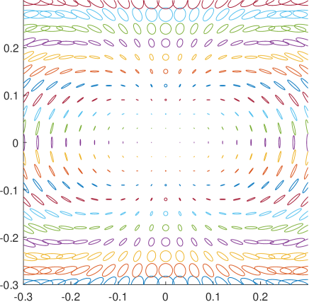
Figure 4. Geodesic discs in the metric of Example2.7 are ellipses shrinking anisotropically towards the origin.
Example 2.8.
Let be the graph of the scalar function , for .
One checks that Gaussian/Ricci curvature when ,
so the Ricci curvature is bounded below,
but the injectivity radius is not bounded away from zero. Indeed, as discussed in [AMR22, §2.1],
the geometric hypothesis in [AMR22, Theorem 1.1] implies in particular
that geodesic balls of radius are Lipschitz diffeomorphic to Euclidean balls. But this is not true in this example,
so [AMR22] does not apply to this manifold.
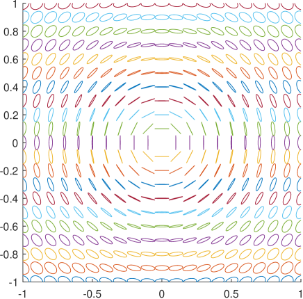
Figure 5. Geodesic discs in the metric of Example2.8 for .
3. Matrix degenerate Boundary Value Problems
We show in this final section how the methods in this paper yield
solvability estimates of elliptic Boundary Value Problems (BVPs) for matrix-degenerate divergence form equations
(3.1)
on a compact manifold with Lipschitz boundary .
We assume that there exists a matrix weight
that describe the degeneracy of the coefficients ,
in the following way.
Lemma 3.1.
color=blue!20]move to the prelims?
Let be a matrix weight and let be a multiplication operator.
The following are equivalent:
•
is uniformly bounded and accretive;
•
is -bounded and -accretive;
•
for all vectors we have
(3.2)
A weak solution to (3.1) is a function such that ,
where is the tangent bundle on .
Since the weighted space ,
then and , so by Poincaré inequality.
Further we assume given a closed Riemannian manifold and, for , a bi-Lipschitz map
between a finite part of the cylinder and a neighbourhood of the boundary ,
so that . See Figure6.
To analyse a weak solution of (3.1) near ,
we define the pullback on the cylinder .
Then satisfies
(3.3)
with coefficients
where denotes the pushforward via , so is the Piola transformation,
and denotes the pullback via .
See [Rosen2019, §7.2 and Example 7.2.12] for more details on this transformation.
The differential operators in (3.3) are
(3.4)
where denotes the vertical unit vector along the cylinder,
and is the tangetial part of .
Define
the pulled back matrix weight .
Lemma 3.2.
The matrix is uniformly bounded and accretive
on a neighbourhood of the boundary if and only if
is uniformly bounded and accretive on .
Indeed,
the condition (3.2) for and
is seen to be equivalent to (3.2) for and .
To obtain solvability estimates,
we require that the matrix weight has the structure
meaning that is constant along the cylinder
and that the vertical direction is a principal direction of .
The functions and are assumed to be scalar and matrix weights on , respectively.
Using a transformation of coefficients from [AAMc2010],
the divergence form equation (3.3) can be turned into an evolution equation
(3.5)
for the conormal gradient of on the cylinder .
Here is the conormal derivative.
We make this correspondence precise in the following lemma.
Lemma 3.3.
A function is a weak solution to the divergence form equation
if and only if its conormal gradient solves the Cauchy–Riemann system (3.5)
with
The operator is self-adjoint on and is -bounded and -accretive.
Proof.
Consider the transformation of the coefficient given by
This map is an involution and
preserves accretivity and boundedness [AAMc2010, Proposition 3.2].
Following [AAMc2010, AMR22] the divergence form equation (3.3) is equivalent to
(3.6)
Then a computation shows that
(3.7)
We introduce weights into the system (3.6) as following:
where
we used that multiplication by and commute since is independent of .
Using (3.7) we define
The argument of on the right hand side is -bounded and -accretive.
Since preserves accretivity and boundedness,
is uniformly bounded and accretive.
The reader can check that coincides with the expression in the statement of the lemma.
∎
We note that , with and from Lemma3.3,
has the same structure as the operators considered in Section2,
if we replace by a compact manifold .
As in Section2, we use a metric on adapted to the weights :
we assume the existence of a smooth, closed Riemannian manifold
and a -homeomorphism
such that the pullback of
the metric on via
is
and we defined the scalar weight on ,
where denotes the pushforward via .
We extend the map to a map between the corresponding cylinders by setting
The extension of the Riemannian metric on the cylinder
and its pullback via are
(3.8)
In the following, the variable is in , while .
We denote by , and the Riemannian measures on
, and on , respectively. See Figure6.
We also denote by and
the distance functions on and induced by and .
Figure 6. The neighborhood of in is transformed by the bi-Lipschitz map into the cylinder with anisotropic degenerate coefficients .
The coefficients on the cylinder are isotropically degenerate.
Note that is isotropically degenerate, meaning that is a scalar weight in each component.
Weak solutions to the anisotropically degenerate equation (3.3)
correspond to weak solutions to an isotropically degenerate equation on .
Lemma 3.4.
Define the coefficients on the cylinder by
Then is uniformly bounded and accretive.
Moreover, the function on is a weak solution to
(3.9)
if and only if is a weak solution to
(3.10)
on .
Proof.
Define the matrix weight on .
Replacing by in Lemma3.2
shows that is uniformly bounded and accretive.
We have
since and . Thus .
If , then is in
Moreover ,
so the non-smooth Piola transformation in TheoremA.3 shows that
in .
This completes the proof.
∎
Since is isotropically degenerate, we can apply results from [AMR22, §4] to obtain solvability estimates of BVPs for .
One can then translate to matrix-weighted norms on the cylinder and in
to obtain the corresponding results for our BVPs for matrix-degenerate equations.
To illustrate this, we consider the non-tangential maximal Neumann solvability estimate
(3.11)
proved in [AMR22, Theorem 1.4].
In the notation of the present paper, the right hand side of (3.11) is
where is the full gradient of as defined in (3.4).
Note that
As for the left hand side in (3.11),
translating the Banach norm in [AMR22, eq. (4.13)] to our present notation gives
where is a smooth cut-off towards the top of the cylinder,
for example .
Note that in the second term, with abuse of notation, we denoted again by the pullback on .
We recall the definition of the modified non-tangential maximal function used on the cylinder .
Figure 7. Non-tangential approach regions. On the left the -adapted approach regions: in the first at , in the second region .
On the right hand side, the corresponding non-tangential conical approach regions to .
Note that the approach regions for shown in Figure7 left are intimately connected to the failure
of standard off-diagonal estimates for the resolvent of the operator from Lemma3.3.
On the other hand, such off-diagonal estimates do hold for the corresponding operator
associated to , from [AMR22, Proposition 4.2].
And indeed on we have standard non-tangential approach regions on the right in Figure7,
and in [AMR22, Theorem 1.4].
For our solvability result,
we also need the analogue of the Carleson discrepancy from [AMR22, Eq. (4.10)]
for a multiplier on the cylinder with
Whitney regions and balls taken with respect to the distance .
The quantity is given by
where .
Summarising, we have obtained the following solvability result for the Neumann BVP for anisotropically degenerate divergence form equations (3.3).
Theorem 3.6.
Let ,,,,,, , , , and
be as above and summarized in Figure6.
Assume that:
•
and that and are scalar and matrix weights,
•
the matrix degenerate coefficients has trace
such that
(1)
the Carleson discrepancy ,
(2)
is close to its adjoint as operator on ,
with small enough.
Then the Neumann solvability estimate
holds for all weak solutions to in , with near boundary values of , in , as above.
Moreover depends only on ,
and the accretivity constant of ,
other than the structural geometric constants of :
dimension, injectivity radius and lower bound on the Ricci curvature.
Proof.
Apply [AMR22, Theorem 1.4] to the isotropically degenerate equation (3.9) on
(see Figure6). Translation of this result to the anisotropically degenerate equation
in (and the Lipschitz equivalent equation on the cylinder , near )
gives the stated result.
We have seen above the translation of the solvability estimate.
The translation of the Carleson discrepancy and almost self-adjointness hypothesis is done similarly
using Lemma3.2 with replaced by
and a change of variables in the integrals.
∎
The solvability estimates for the Dirichlet and Dirichlet regularity BVPs from [AMR22, Theorem 1.4]
and the Atiyah–Patodi–Singer BVPs from [AMR22, Theorems 4.5,4.6] can similarly be extended to anisotropically degenerate equations.
We leave the details to the interested reader.
Appendix A pullbacks and Piola transformations
We generalise the commutation theorem [RosenGMA, Theorem 7.2.9, Lemma 10.2.4]
for external derivatives and pullbacks to homeomorphisms and weighted fields.
(We only deal with the scalar and vector case which we need).
Throughout this section,
is assumed to be a homeomorphism,
meaning that , are continuous with weak Jacobian matrix , in .
Theorem A.1(Change of variables).
If is a homeomorphism then
holds for all integrable, compactly supported functions .
This holds for homeomorphism ,
as readily seen by mollifying and passing to the limit.
We first extend to non-smooth :
Theorem A.2(Non-smooth chain rule).
Assume and is compactly supported with weak gradient .
Let be a homeomorphism.
Define the weights
and assume .
Then has weak gradient
Proof.
Mollify ,
so that .
It follows that in and in
using dominated convergence and bounds for
the vector Hardy–Littlewood maximal operator introduced by Christ and Goldberg [ChristGoldberg01],
see [Goldberg03, Theorem 3.2].
Note that and
.
Apply the chain rule (A.1) to and for a fixed test function .
We can pass to the limit in and conclude since
the left hand side of (A.1) is bounded as
where the first integral is on the compact support of
and we used TheoremA.1 when changing variables.
For the right hand side in (A.1),
using that , we bound
We refer to the transformation applied to on the right hand side of (A.2)
as the Piola transformation ,
where denotes the pushforward via .
This transformation is the adjoint of the pullback with respect to the unweighted pairing.
We extend identity (A.2) to non-smooth vector fields .
Theorem A.3(Non-smooth Piola transformation).
Assume that and is compactly supported with
weak divergence .
Let be a homeomorphism.
Define the weights
and assume .
Then
and has weak divergence
The proof is analogous to the one of TheoremA.2,
where we pass to the limit in (A.2).
Acknowledgements
G.B. is supported by the Knut and Alice Wallenberg foundation,
KAW grant 2020.0262 postdoctoral program in Mathematics for researchers from outside Sweden.
A.R. was supported by Grant 2022-03996 from the Swedish research council, VR.
References
[AAM10]Pascal Auscher, Andreas Axelsson and Alan McIntosh
“Solvability of elliptic systems with square integrable boundary data”
In Ark. Mat.48.2, 2010, pp. 253–287
DOI: 10.1007/s11512-009-0108-2
[ADM96]David Albrecht, Xuan Duong and Alan McIntosh
“Operator theory and harmonic analysis”
In Instructional workshop on analysis and geometry, Canberra, Australia, January 23 - February 10, 1995. Part III: Operator theory and nonlinear analysisCanberra: Australian National University, Centre for Mathematics and its Applications, 1996, pp. 77–136
[AKM06]Andreas Axelsson, Stephen Keith and Alan McIntosh
“Quadratic estimates and functional calculi of perturbed Dirac operators”
In Invent. Math.163.3, 2006, pp. 455–497
DOI: 10.1007/s00222-005-0464-x
[AMN97]Pascal Auscher, Alan McIntosh and Andrea Nahmod
“The square root problem of Kato in one dimension, and first order elliptic systems”
In Indiana Univ. Math. J.46.3, 1997, pp. 659–695
DOI: 10.1512/iumj.1997.46.1423
[AMR22]Pascal Auscher, Andrew J Morris and Andreas Rosén
“Quadratic estimates for degenerate elliptic systems on manifolds with lower Ricci curvature bounds and boundary value problems”
In arXiv:2209.11529, 2022
[ARR15]Pascal Auscher, Andreas Rosén and David Rule
“Boundary value problems for degenerate elliptic equations and systems”
In Ann. Sci. Éc. Norm. Supér. (4)48.4, 2015, pp. 951–1000
DOI: 10.24033/asens.2263
[Aus+02]Pascal Auscher et al.
“The solution of the Kato square root problem for second order elliptic operators on .”
In Ann. Math. (2)156.2, 2002, pp. 633–654
DOI: 10.2307/3597201
[BLM17]Kelly Bickel, Katherine Lunceford and Naba Mukhtar
“Characterizations of matrix power weights”
In J. Math. Anal. Appl.453.2, 2017, pp. 985–999
DOI: 10.1016/j.jmaa.2017.04.035
[Bow01]Marcin Bownik
“Inverse volume inequalities for matrix weights”
In Indiana Univ. Math. J.50.1, 2001, pp. 383–410
DOI: 10.1512/iumj.2001.50.1672
[Cal77]A.. Calderon
“Cauchy integrals on Lipschitz curves and related operators”
In Proc. Natl. Acad. Sci. USA74, 1977, pp. 1324–1327
DOI: 10.1073/pnas.74.4.1324
[CG01]Michael Christ and Michael Goldberg
“Vector weights and a Hardy-Littlewood maximal function”
In Trans. Am. Math. Soc.353.5, 2001, pp. 1995–2002
DOI: 10.1090/S0002-9947-01-02759-3
[CMM82]R.. Coifman, A. McIntosh and Y. Meyer
“L’intégrale de Cauchy définit un opératuer borne sur pour les courbes lipschitziennes”
In Ann. Math. (2)116, 1982, pp. 361–387
DOI: 10.2307/2007065
[CMR18]David Cruz-Uribe, José María Martell and Cristian Rios
“On the Kato problem and extensions for degenerate elliptic operators”
In Anal. PDE11.3, 2018, pp. 609–660
DOI: 10.2140/apde.2018.11.609
[CR15]David Cruz-Uribe and Cristian Rios
“The Kato problem for operators with weighted ellipticity”
In Trans. Am. Math. Soc.367.7, 2015, pp. 4727–4756
DOI: 10.1090/S0002-9947-2015-06131-5
[Dav84]Guy David
“Opérateurs intégraux singuliers sur certaines courbes du plan complexe”
In Ann. Sci. Éc. Norm. Supér. (4)17, 1984, pp. 157–189
DOI: 10.24033/asens.1469
[Gol03]Michael Goldberg
“Matrix weights via maximal functions.”
In Pac. J. Math.211.2, 2003, pp. 201–220
DOI: 10.2140/pjm.2003.211.201
[Haj93]Piotr Hajłasz
“Change of variables formula under minimal assumptions”
In Colloq. Math.64.1, 1993, pp. 93–101
DOI: 10.4064/cm-64-1-93-101
[Kat61]Tosio Kato
“Fractional powers of dissipative operators”
In J. Math. Soc. Japan13, 1961, pp. 246–274
DOI: 10.2969/jmsj/01330246
[Kat95]Tosio Kato
“Perturbation theory for linear operators.”, Class. Math.
Berlin: Springer-Verlag, 1995
[KM85]C. Kenig and Y. Meyer
“Kato’s square roots of accretive operators and Cauchy kernels on Lipschitz curves are the same”, Recent progress in Fourier analysis, Proc. Semin., El Escorial/Spain 1983, North-Holland Math. Stud. 111, 123-143 (1985)., 1985
[Lac+14]Michael T. Lacey, Eric T. Sawyer, Chun-Yen Shen and Ignacio Uriarte-Tuero
“Two-weight inequality for the Hilbert transform: a real variable characterization. I”
In Duke Math. J.163.15, 2014, pp. 2795–2820
DOI: 10.1215/00127094-2826690
[MQ91]Alan McIntosh and Tao Qian
“Convolution singular integral operators on Lipschitz curves”
In Harmonic analysis. Proceedings of the special program at the Nankai Institute of Mathematics, Tianjin, PR China, March-July, 1988Berlin etc.: Springer-Verlag, 1991, pp. 142–162
[Ros19]Andreas Rosén
“Geometric multivector analysis. From Grassmann to Dirac”, Birkhäuser Adv. Texts, Basler Lehrbüch.
Cham: Birkhäuser, 2019
DOI: 10.1007/978-3-030-31411-8