GNNavigator: Towards Adaptive Training of Graph Neural Networks via Automatic Guideline Exploration

Abstract.

Graph Neural Networks (GNNs) succeed significantly in many applications recently. However, balancing GNNs training runtime cost, memory consumption, and attainable accuracy for various applications is non-trivial. Previous training methodologies suffer from inferior adaptability and lack a unified training optimization solution. To address the problem, this work proposes GNNavigator, an adaptive GNN training configuration optimization framework. GNNavigator meets diverse GNN application requirements due to our unified software-hardware co-abstraction, proposed GNNs training performance model, and practical design space exploration solution. Experimental results show that GNNavigator can achieve up to 3.1$\times$ speedup and 44.9% peak memory reduction with comparable accuracy to state-of-the-art approaches.

1. Introduction

Graph neural networks (GNNs) have attained significant success across a wide range of graph-based applications, such as node classification (kipf2017semi, ; velivckovic2018graph, ), link prediction, community detection and flow forecasting. Thanks to the information propagation along edges, GNNs exhibit the ability to capture intricate patterns and relationships within graph data, significantly surpassing traditional deep learning approaches. However, due to neighborhood explosion, GNNs face more serious challenges than traditional deep learning in terms of accuracy, execution time. Many efforts have been made to address the challenges, which can be generally categorized based on their optimization goals as accuracy centric optimization, time efficiency centric optimization, and memory footprint optimization. To minimize feature retrieving traffic, PaGraph (lin2020pagraph, ) and BGL (liu2023bgl, ) introduce feature caching policies, utilizing free GPU memory for caching. Works such as FastGCN (chen2018fastgcn, ), GraphSAINT (zeng2019graphsaint, ) leverage the locality of graph data for more efficient neighbor sampling (liu2022gnnsampler, ). To enhance GNNs computation performance, (chen2020fusegnn, ; wang2021gnnadvisor, ) develop GPU kernels and thread assignment policies, while (you2022gcod, ) design accelerators for GNNs training. Additionally, there are many other works focused on optimizations such as workflow pipelining (kaler2022accelerating, ), dedicated task scheduling (yang2022gnnlab, ), and feature data compression (liu2021exact, ).

Unfortunately, all aforementioned optimization strategies are not sufficient for tackling existing problems. Firstly, without a comprehensive view of GNNs training, most existing approaches perform well only under specific scenarios. As depicted in Fig. 1, existing works typically achieve their claimed excellent performance by making trade-offs among different metrics. The speedup of PaGraph (lin2020pagraph, ) largely depends on the extra consumption of memory resources. And compared to PaGraph (lin2020pagraph, ), 2PGraph (zhang20212pgraph, ) achieves 2.45$\times$ speedup at the cost of a 3% drop in training accuracy. The adaptability of existing works becomes limited when confronted with diverse application requirements and scenario constraints. Secondly, the collaboration among different optimization strategies is disappointing. Regardless of the difficulties in strategies combination, simply linking multiple strategies may compromise their performance due to incompatibility. Finally, many previous works need careful adjustments in configuration to ensure their performance. This process largely relies on essential expertise and requires significant human effort. To this end, enabling automatic exploration for adaptive solutions with low overhead is valuable, according to the varying requirements of graph-based applications.

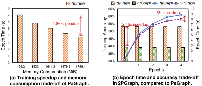
Figure 1. Profiling on existing GNN training frameworks.

In this paper, we introduce a novel GNNs training framework called GNNavigator. GNNavigator can automatically generate effective training guidelines based on application requirements. Our approach distinguishes itself from other GNNs training optimizations by its adaptability to applications prioritizing different performance metrics. Furthermore, many existing optimization strategies can be easily reproduced through simple reconfiguration within GNNavigator framework. Consequently, GNNavigator always achieves excellent performance comparable to or better than previous works.

Our contributions are summarized as follows:

• Unified optimizations abstraction. We decompose GNNs training into several components, categorizing and abstracting various optimizations according to the decomposition.

• Reconfigurable runtime backend. Upon the abstractions, we build a reconfigurable runtime backend to support diverse optimizations by simply reconfiguring.

• “Gray-box” performance estimating model. We construct a ”gray-box” model, combining theoretical analysis and machine learning, for accurate GNNs training performance estimation.

• Adaptive training guidelines. With the assistance of performance estimation, GNNavigator provides training guidelines adaptive to application requirements automatically.

2. Background and Motivations

In this section, we outline the problem boundaries of GNNavigator in Sec. 2.1 and Sec. 2.2, and discuss the motivations inspired by several key observations in GNNs training in Sec. 2.3.

2.1. Mini-batch based GNNs Training

0:  graph $G(\mathcal{V},\mathcal{E})$, batch size $|\mathcal{B}^{0}|$, initial graph network $M(L,\Phi_{init})$, network layers $L$, network parameters $\Phi$. 10:  converged graph network $M(L,\Phi_{trained})$. 21:  for $i$ in [0, $|\mathcal{V}|/|\mathcal{B}^{0}|)$ do   $\triangleright$ Component 1: Sampling on Host 32:     $G_{i}(\mathcal{V}_{i},\mathcal{E}_{i})\leftarrow\textbf{SubgraphSampling}(G(\mathcal{V},\mathcal{E}),\mathcal{B}^{0}_{i})$   $\triangleright$ Component 2: Transmission 43:     $\textbf{MemcpyHtoD}(G_{i})$   $\triangleright$ Component 3: Computation on Device 4:     for $l$ in $L$ do 5:       $a^{l}\leftarrow\textbf{Aggregate}(G_{i},M)$ 6:       $h^{l}\leftarrow\textbf{Combine}(a^{l},M)$ 7:       $loss\leftarrow\textbf{LossFunction}(h^{l},G_{i})$ 8:       $\textbf{Backwards}()$ 9:     end for 10:  end for 11:  $\textbf{MemcpyDtoH}(M(L,\Phi_{trained}))$ 12:  return $M(L,\Phi_{trained})$

Algorithm 1 Mini-batch based GNNs training on heterogeneous platforms.

The computation of GNNs can typically be described by their aggregate function and combine function. On a graph $G(\mathcal{V},\mathcal{E})$ with vertex set $\mathcal{V}$ and edge set $\mathcal{E}$. $v\in\mathcal{V}$ is a vertex in graph whose feature vector is $h^{0}_{v}$, and $\mathcal{N}(v)$ represents its neighborhood. Let $e^{l-1}_{uv}$ be the edge feature at layer $l-1$. The computation of a single GNN layer $l$ can be formulated as:

(1) $$\begin{split}&a_{v}^{l}=\textbf{Aggregate}^{l}\left(h^{l-1}_{u},e^{l-1}_{uv}|u\in\mathcal{N}(v)\cup h^{l-1}_{v}\right),\\ &h_{v}^{l}=\textbf{Combine}^{l}(a_{v}^{l}),\end{split}$$

where $a_{v}^{l}$ is the aggregate result and $h_{v}^{l}$ is the vertex embedding of $v$ at layer $l$. By stacking multiple GNN layers together, we can get the final output of graph neural networks (qi2023architectural, ).

To enable GNNs training on tremendously large-scale graphs, mini-batch based training has been introduced. It conducts training on subgraphs iteratively, to alleviate the ever-increasing requirements in memory. Mini-batch based training first samples a subgraph $G_{i}(\mathcal{V}_{i},\mathcal{E}_{i})$ from $G(\mathcal{V},\mathcal{E})$ as mini-batch, and then train the network on a series of mini-batches.

2.2. Heterogeneous Platforms for GNNs Training

GNN training has been explored across diverse hardware platforms. The two most influential frameworks, PyG (Fey/Lenssen/2019, ) and DGL (wang2019dgl, ), both support GNNs training on heterogeneous architectures like CPU-GPU. Aligraph and Euler (zhu2019aligraph, ) focus on CPU-only platforms to enable flexible computation patterns. Many other works use FPGAs (lin2023hitgnn, ; lin2022hp, ) or even accelerators (you2022gcod, ; zhou2023hardware, ) as computation platforms, leading to a notable reduction in time cost or energy consumption.

However, regardless of the diversity in hardware, it is still the mainstream to train GNNs with heterogeneous platforms. As illustrated in Algo. 1, complex operations such as sampling and file I/O, are executed on general-proposed platforms such as CPUs, which we call host. Massive but simple operations such as aggregate and combine are conducted on dedicated designed platforms such as GPUs or FPGAs, which we call device. Furthermore, host and device can exchange data through host-device links, which can be implied through PCIe or DMA. Remarkably, based on the assumption that data retrieving within a certain platform is always much faster than fetching data from another platform through data links, redundant memory resources on device can be treated as a cache to store partial graph data, aiming to accelerate GNNs training (lin2020pagraph, ; liu2023bgl, ).

2.3. Observations and Opportunities

Algo. 1 lists the overview of mini-batch based GNNs training on heterogeneous platforms. The number of mini-batches $|\mathcal{V}|/|\mathcal{B}^{0}|$ is decided in line $1$. Given the target vertices set $\mathcal{B}^{0}_{i}$ of each iteration, the mini-batch $G_{i}(\mathcal{V}_{i},\mathcal{E}_{i})$ is deduced according to the specific sampling algorithm (line $2$). The sampled subgraph is then transferred to device through links between host and device (line $3$). Then, GNNs are trained on device across the sampled mini-batches (line $4$ to $8$). The trained model is transferred back to host for further processing (line $11$).

We outline $4$ categories of training optimization opportunities based on Algo. 1, i.e., sampling, transmission, computation, and model design. Three requirements are summarized, given the limitations of previous related approaches.

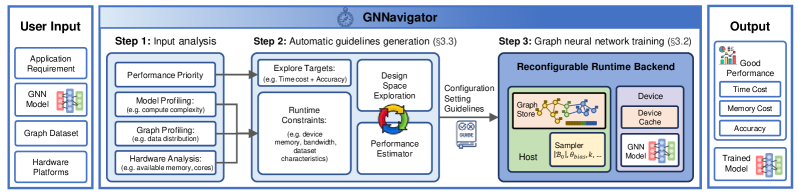
Figure 2. Framework overview of GNNavigator.

Compatibility. The framework should be compatible with many dedicatedly designed GNN training optimizations. For example, FPGA-orient optimization (lin2022hp, ) is orthogonal to GNNAdvisor (wang2021gnnadvisor, ). However, compatibility permits a feasible joint optimization by combining these two methodologies.

Adaptability. The framework should be adaptable to various applications. Different GNN applications pertain to various characteristics, emphasizing runtime performance or hardware budgets. It is non-trivial to find a sweet one-for-all solution. Adaptability allows the framework to produce optimal training optimization strategies given different scenarios.

Automation. The framework should be automated. The automation alleviates heavy labor force input in deciding optimal training optimization parameters. Inspired by BOOM-Explorer (bai2021boom, ), we formulate the automation process as a design space exploration (DSE) problem and solve it via our customized surrogate model.

3. GNNavigator Framework

Motivated by the observations and opportunities outlined in Sec. 2.3, we introduce GNNavigator, an adaptive framework automatically fine-tuning GNNs training according to application requirements and hardware constraints. GNNavigator is constructed upon three pivotal techniques: 1) a unified and reconfigurable backend facilitating efficient strategy cooperation, 2) a ”gray-box” performance estimator, and 3) an application-driven design space exploration tailored to requirements and constraints.

3.1. Framework Overview

Fig. 2 provides an overview of GNNavigator, and its general workflow. For better adaptability, GNNavigator requires some essential information, typically related to the applications, as input.

Users should specify the following input items:

• The graph dataset $G(\mathcal{V},\mathcal{E})$ to be trained on.

• The GNN model $M(L,\Phi_{init})$, with explicit network architecture.

• The application requirements like time cost $T$, memory consumption $\Gamma$, accuracy $Acc$, etc., along with the user-defined priorities for different requirements.

• The heterogeneous hardware platforms for GNNs training.

The user inputs are quantitatively analyzed to formulate the parameterized explore targets and runtime constraints, as shown in Step 1. Then, in Step 2, GNNavigator automatically generates GNN training guidelines, taking both explore targets and runtime constraints into account to ensure its adaptability. We further design a ”gray-box” performance estimator to accurately predict the training performance with relatively low overhead. Users receive the guidelines, in the form of training configuration settings, and apply these settings on GNNavigator’s runtime backend for GNNs training (Step 3). GNNavigator guarantees that the actual training performance $Perf\{T,\Gamma,Acc\}$, measured in terms of time cost $T$, memory consumption $\Gamma$, and accuracy $Acc$, not only satisfies application requirements but also outperforms other handcrafted designs.

3.2. Unified Abstraction of Training Optimizations

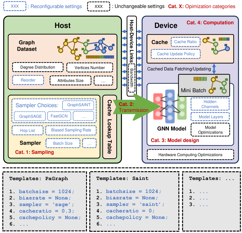
Figure 3. Reconfigurable runtime backend of GNNavigator.

The various GNNs training optimizations can be generally classified into four categories: sampling strategies, transmission strategies, computation optimizations, and model design optimizations, according to the decomposition of Algo. 1, as introduced in Sec. 2.3. Unified abstractions for optimizations in each category are generated respectively. Furthermore, as shown in Fig. 3, a reconfigurable runtime backend is established based on the categorizations and abstractions, with optimizations from different categories mapping to different parts of the backend.

Sampling strategies. There are node-wise samplers, layer-wise samplers, and subgraph-wise samplers for unbiased sampling (liu2022gnnsampler, ), and dedicated designed locality-aware samplers aiming for biased sampling (zhang20212pgraph, ). Despite the diversity in sampling strategies, samplers generally expand a subgraph from given target vertex set. Therefore, we can provide a unified abstraction of sampling strategies, that is, samplers iteratively fanout vertices at certain probability, and further generate subgraphs.

In our abstraction of samplers, it receives a certain number of target vertices $\mathcal{B}_{i}^{l-1}$ as input from layer $l-1$, and fanouts $k^{l}$ neighbors from every vertex $v_{i}^{l-1}\in\mathcal{B}_{i}^{l-1}$ at a given probability. The output $\mathcal{B}_{i}^{l}$ at layer $l$ can be formulated as follows:

(2) $$\mathcal{B}^{l}_{i}=\bigcup_{v_{i}^{l-1}\in\mathcal{B}^{l-1}_{i}}u\cdot\mathbb{I}_{p(\eta)}\left(\frac{k^{l}}{|\mathcal{N}(v_{i}^{l-1})|}\right),u\in\mathcal{N}(v_{i}^{l-1}).$$

$\mathbb{I}_{p(\eta)}$ is an indicator function to decide whether to select a neighbor $u$, according to a probability $p(\eta)$ specified by the sampling algorithm.

While Eq. 2 is primarily in the form of node-wise sampling, it can generalize other sampling strategies as well. For instance, in the case of layer-wise sampling (chen2018fastgcn, ), the number of sampled nodes at layer $l$ can be represented as $\Delta^{l}$, which is a predetermined value. We can derive the mathematical expectation of $k^{l}$ from $\Delta^{l}$ by:

(3) $$\mathbb{E}(k^{l})=\frac{\Delta^{l}}{|\mathcal{B}_{i}^{l-1}|}\cdot\mu\left(p(\eta),\mathcal{B}_{i}^{l-1}\right),$$

where $\mu(p(\eta),\mathcal{B}_{i}^{l-1})$ is a coefficient which indicates the probability of multi-vertices in $\mathcal{B}_{i}^{l-1}$ shares a common neighbor in $\mathcal{B}_{i}^{l}$. In this way, layer-wise sampling has been uniformly abstract as Eq. 2. Locality-aware sampling and subgraph-wise sampling can be more easily integrated into the abstraction, according to their sampling patterns. By setting the neighbor selection probability to a function of data locality $p(\eta)$, we can reproduce biased samplers that prefer a certain subset of $\mathcal{V}$. Subgraph-wise sampling strategies like GraphSAINT (zeng2019graphsaint, ) can be viewed as a special case of node-wise sampling, with many more hops, but only a single neighbor fanout in each hop. To this end, we can unify different sampling strategies to the sampler in Fig. 3, with configurable settings being enumerated

Transmission strategies. Regardless of the implementation of transmission strategies, they always ensure the required data being on the device when computing. Note that not all required data needs transmission. An abstraction can be drawn, according to the gap between the required data volume and actual transferred data volume. The transmission strategies typically leverage the free memory resources on device as a cache to alleviate redundant data transmission. Despite their substantial differences in cache updating policies, we can consistently abstract them as follows. First, the device cache is initialized according to the available memory resource on device. Given a mini-batch, the device cache figures out which part of the mini-batch has been cached. The remaining part is filtered out from the host and transferred to the device through host-device links. With all essential data on device, training on the mini-batch can be conducted. Finally, the device cache is updated according to the cache updating policy. Uniformly, part of the configurable settings on transmission are listed in the device cache in Fig. 3. We can distinguish different transmission strategies by configuring the settings properly.

Computation and model design optimizations. GNN models typically embed graph topological information through aggregate functions and enable feature learning by combine functions. Let along the detailed design of models, abstraction of model design optimizations can be formulated based on the time complexity and spatial complexity of aggregate and combine functions, as shown in Eq. 1. Similarly, computation optimizations are abstracted by their maximum throughput and available memory resources. Although the computation optimizations show significant diversity in their targeting device platforms, ranging from GPUs to FPGAs, we find that they can all be measured by their computing capability and available resources.

In Fig. 3, both computation optimizations and model design optimizations are mapped to the device, for actual execution and the following performance estimation.

Reconfigurable runtime backend. Thanks to its reconfigurability, the runtime backend can represent itself with diverse performance, making it adaptive to a wide range of applications.

Fig. 3 depicts the mapping relationships between the four optimization categories and backend components, marked by red words. Within each backend component, there are many reconfigurable settings that can be freely adjusted to simulate existing approaches, marked with blue dash-line rectangles. For instance, by disabling cache update policy, and properly configuring the cache ratio, the backend generally reproduces the approach proposed in PaGraph (lin2020pagraph, ). Similarly, many existing works can be conveniently reproduced, by applying the configurations setting templates shown in Fig. 3 Furthermore, the unified runtime backend allows for a flexible combination of optimizations from different categories and greatly outperforms existing works in its compatibility. Note that the runtime backend can even incrementally support future optimizations only if they submit to our abstraction. Additionally, all reconfigurable parameters in the runtime backend make up the design space, which will be discussed in detail in Sec. 3.3.

3.3. Automatic Guidelines Generation

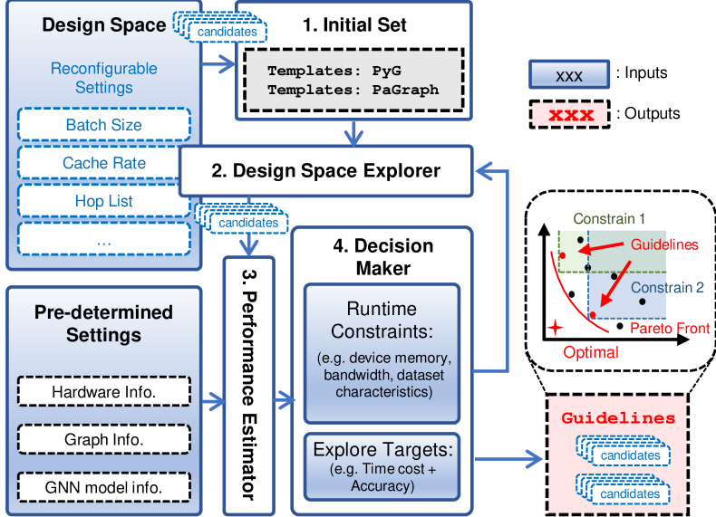
Figure 4. Automatic guidelines exploration.

GNNavigator leverages multi-objective design space exploration (DSE) to automatically generate the training guidelines, as shown in Fig. 4. It benefits from multi-objective DSE in two key aspects. Firstly, in terms of fine-tuning GNN training, the substantial burden of human labor is mitigated through automatic exploration. Secondly, in terms of adaptability, the explorer generates guidelines that satisfy user demands by emphasizing different explore targets. Notably, all the reconfigurable settings in Fig. 3 constitute the design space, represented by blue dash-line rectangles. Moreover, to accelerate the exploration, a ”gray-box” performance estimator is established based on the unified abstractions of optimization strategies.

Gray-box performance estimator. The estimator predicts GNN training performance in a ”gray-box” manner, combining purely theoretical analysis (white-box) and machine learning methods (black-box) together.

As shown in Fig. 4, the estimator makes predictions based on 1) the specific values of all configurable settings, which will be represented as candidate in design space in our following illustration and 2) the pre-determined settings in runtime, usually determined by applications. To ensure the accuracy of estimation, the estimator first theoretically analyzes the data dependence between its inputs and performance $Perf\{T,\Gamma,Acc\}$. Considering the complexity and randomness of graph, black-box models based on machine learning are introduced to estimate some key intermediate variables that influence $T$, $\Gamma$, and $Acc$. We will present the methodology of constructing ”gray-box” models on performance $Perf$ as follows.

Note that the operations on device are independent of those on host. The epoch time can be formulated as:

(4) $$T=n_{iter}\cdot max\left(t_{sample}+t_{transfer},t_{replace}+t_{compute}\right),$$

where $t_{sample}$, $t_{transfer}$, $t_{replace}$, $t_{compute}$ represent the time cost of sampling, transmission, cache updating, and computation on device, respectively, and $n_{iter}$ is the number of mini-batches within an epoch. Let us begin with $t_{replace}$. In scenarios requiring cache replacement, the cache updating overhead is mainly influenced by cache volume $r\cdot|\mathcal{V}|$, and volume of replaced stale data $|\mathcal{V}_{i}|(1-hit)$.

(5) $$t_{replace}=f_{replace}\left(r|\mathcal{V}|,|\mathcal{V}_{i}|(1-hit),Device\right).$$

The $hit$ represents the average cache hit rate, and we use $Host$ $Device$ to indicate the hardware information of host and device respectively.

In a similar fashion, $t_{transfer}$ is determined by the volume of data awaiting transmission $n_{attr}|\mathcal{V}_{i}|(1-hit)$. $t_{sample}$ is primarily affected by changes in subgraph size $|\mathcal{V}_{i}|-|\mathcal{B}^{0}|$, which represents the transition from the original target vertices to the final mini-batch. Lastly, mini-batch size $|\mathcal{V}_{i}|$ and the GNN model $M(L,\Phi)$ together determine $t_{compute}$. We demonstrate the formulations of $t_{replace}$, $t_{transfer}$, and $t_{sample}$ as follows:

(6) $$t_{transfer}=f_{transfer}(n_{attr}|\mathcal{V}_{i}|(1-hit),Host,Device),$$

(7) $$t_{sample}=f_{sample}(|\mathcal{V}_{i}|-|\mathcal{B}^{0}|,Host),$$

(8) $$t_{compute}=f_{compute}(\mathcal{V}_{i},M,Device).$$

The term $n_{attr}$ denotes the attribute dimensions of an individual node.

Remarkably, the functions $f_{compute}$, $f_{replace}$, $f_{transfer}$, and $f_{sample}$ can all be estimated using a pre-trained black-box model. In this way, the performance estimator can predict the execution time of GNN training with negligible latency.

The prediction of device memory consumption $\Gamma$, can also be decomposed to sub-tasks of estimating $\Gamma_{model}$, $\Gamma_{cache}$, $\Gamma_{runtime}$ respectively,

(9) $$\Gamma=\Gamma_{model}+\Gamma_{cache}+\Gamma_{runtime},$$

where $\Gamma_{model}$, $\Gamma_{cache}$, $\Gamma_{runtime}$ are formulated as follows:

(10) $$\begin{split}&\Gamma_{model}\propto|\Phi|,\\ &\Gamma_{cache}=f_{cache}(r|\mathcal{V}|n_{attr}),\\ &\Gamma_{runtime}=f_{runtime}(\overline{|\mathcal{V}_{i}|},\Phi).\end{split}$$

$\Gamma_{model}$ reveals the static memory consumption of GNNs, directly related to $|\Phi_{init}|$. $\Gamma_{cache}$ represents the cache memory consumption, and $\Gamma_{runtime}$ indicates the memory footprint of mini-batch computation phrase.

Estimation of model accuracy falls back behind the ones on the other two metrics in its explainability. Nevertheless, we try to analyze it from the perspective of data distribution. Taking the training accuracy on mini-batches with unbiased sampling as the baseline, the estimator measures the accuracy changes $\delta_{Acc}$ of training as:

(11) $$\delta_{Acc}=f_{accuracy}(Deg(G_{i}),Deg(G),|\mathcal{V}_{i}|).$$

The formulation on accuracy changes is established upon the assumption that a mini-batch will learn more information about a given graph $G$ by focusing on the vertices with more importance. However, the prediction on accuracy is still more like a black box, compared with $T$ and $\Gamma$.

Notably, as can be witnessed in the theoretical analysis, the mini-batch size $|\mathcal{V}_{i}|$ plays an important role in performance estimation. Considering its significance, we analytically formulate the expectation of mini-batch size $\mathbb{E}(|\mathcal{V}_{i}|)$ as:

(12) $$\mathbb{E}\left(|\mathcal{V}_{i}|\right)=f_{overlapping}\left(|\mathcal{B}^{0}|\prod^{L}_{l=1}{(1+k^{l})^{\tau}},p(\eta)\right).$$

where $f_{overlapping}$ is a penalty function determined by graph characteristics and is certainly learnable. Consequently, we obtain an extremely accurate prediction of mini-batch size by Eq. 12, far better than the pure black-box model (Decision Tree Regression), as shown in Fig. 5. The predicted values and the measured values are more consistent with the equal line, which is marked with red dash-line.

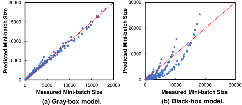
Figure 5. Accuracy comparison between different estimator models. The distance between each blue point and the red dash-line reflects the estimator’s accuracy

Application-driven design space exploration. Based on GNNavigator’s precise estimation of performance, we can conduct the design space exploration that is adaptive to hardware constraints and application requirements.

As shown in Fig. 4, the explorer starts its exploration from an initial candidates configured according to templates of existing works, to ensure the generated guidelines could achieve at least a comparable performance to previous approaches. Then, it travels across all configurable settings, with the depth-first-search (DFS) algorithm. The explorer iteratively tries candidates in design space and gets the performance of candidates through the performance estimator. According to the explore targets, the decision maker determines whether to accept a candidate as the guideline or to continue the exploration. Notably, some runtime constraints are imposed according to different applications. The explorer will prune the design space to accelerate the process of exploration when the estimated performance cannot satisfy the runtime constraints. With an awareness of application requirements, the explorer emphasizes the specific performance metrics and leverages Pareto front theory to obtain the most suitable candidates, which are finally provided as training guidelines.

4. Experimental Results

4.1. Evaluation Setup

Baselines. To evaluate the effectiveness of GNNavigator, we consider 3 baselines: PyG (Fey/Lenssen/2019, ), a state-of-the-art GNN framework on both CPUs and GPUs; PaGraph (lin2020pagraph, ), a GNNs computation framework with static cache; 2PGraph (zhang20212pgraph, ), a CPU-GPU heterogeneous framework, with cache-aware sampling to accelerate training. PaGraph (lin2020pagraph, ), 2PGraph (zhang20212pgraph, ), and original PyG (Fey/Lenssen/2019, ) are all reproduced on our runtime backend for a fair comparison. The reproductions achieve similar results as the ones they report. Note that the volume of available GPU memory will significantly influence the performance of PaGraph (lin2020pagraph, ). Therefore, we measure the performance of PaGraph (lin2020pagraph, ) under ideal circumstances (Pa-Full) and resource-limited circumstances (Pa-Low) respectively.

Datasets and platforms. Our experiments are conducted on datasets with various scales, including Ogbn-arxiv (AR), Ogbn-products (PR) (hu2020ogb, ), Reddit2 (RD2), and representative graph neural networks, including GCN, GAT, GraphSAGE (SAGE). We test the performance of the runtime backend on different devices such as RTX 4090, A100, and M90, and further set manual constraints to simulate various scenarios of application. The time cost and memory footprint are measured by PyTorch profiler (paszke2019pytorch, ).

Performance estimator settings. The performance estimator is trained on the ground-truth performance covering the whole design space. For fairness, the estimator is established upon the performance across all the datasets available, except the one waiting for estimation. Specifically, to embed more prior knowledge, we randomly generate some power-law graphs and profile the training on them as data enhancement to optimize our performance estimator.

Table 1. Performance of GNNavigator across different tasks.

Applications (Dataset+Model)	Method	Time ($T$)/s	Memory ($\Gamma$)/GB	Accuracy ($Acc$)
PR + SAGE	PyG (Fey/Lenssen/2019, )	9.27	1.25	90.55%
	Pa-Full (lin2020pagraph, )	5.44(1.7$\times\uparrow$)	2.11(69.1$\%\uparrow$)	90.42%
	Pa-low (lin2020pagraph, )	8.39(1.1$\times\uparrow$)	1.34(7.5$\%\uparrow$)	90.58%
	2P (zhang20212pgraph, )	5.18(1.8$\times\uparrow$)	0.88(29.7$\%\downarrow$)	90.36%
	Bal	3.67(2.5$\times\uparrow$)	1.23(7.5$\%\downarrow$)	91.19%
	Ex-TM	3.95(2.3$\times\uparrow$)	0.78(37.3$\%\downarrow$)	90.37%
	Ex-MA	5.12(1.8$\times\uparrow$)	0.88(29.7$\%\downarrow$)	91.22%
	Ex-TA	3.59(2.6$\times\uparrow$)	1.64(31.1$\%\uparrow$)	91.24%
RD2 + SAGE	PyG (Fey/Lenssen/2019, )	7.68	1.32	79.28%
	Pa-Full (lin2020pagraph, )	3.78(2.0$\times\uparrow$)	1.80(36.3$\%\uparrow$)	79.23%
	Pa-low (lin2020pagraph, )	7.04(1.1$\times\uparrow$)	1.43(7.6$\%\uparrow$)	79.25%
	2P (zhang20212pgraph, )	3.51(2.2$\times\uparrow$)	0.84(36.36$\%\downarrow$)	75.95%
	Bal	3.53(2.1$\times\uparrow$)	0.87(34.1$\%\downarrow$)	80.03%
	Ex-TM	2.45(3.1$\times\uparrow$)	0.98(44.9$\%\downarrow$)	76.42%
	Ex-MA	3.82(2.0$\times\uparrow$)	0.91(31.1$\%\downarrow$)	81.16%
	Ex-TA	2.85(2.7$\times\uparrow$)	0.99(25.0$\%\downarrow$)	79.87%
AR + GAT	PyG (Fey/Lenssen/2019, )	3.49	5.80	61.44%
	Pa-Full (lin2020pagraph, )	2.98(1.2$\times\uparrow$)	5.87(1.3$\%\uparrow$)	61.38%
	Pa-low (lin2020pagraph, )	3.46(1.0$\times\uparrow$)	5.80(0.1$\%\uparrow$)	61.45%
	2P (zhang20212pgraph, )	3.53(1.0$\times\uparrow$)	5.81(0.2$\%\uparrow$)	60.51%
	Bal	2.98(1.2$\times\uparrow$)	5.87(1.3$\%\uparrow$)	61.43%
	Ex-TM	3.21(1.1$\times\uparrow$)	5.84(0.8$\%\uparrow$)	61.07%
	Ex-MA	3.23(1.1$\times\uparrow$)	5.85(0.9$\%\uparrow$)	61.71%
	Ex-TA	2.98(1.2$\times\uparrow$)	5.87(1.3$\%\uparrow$)	61.43%

4.2. Overall Performance

GNNavigator provides guidelines from a comprehensive view of performance $Perf\{T,\Gamma,Acc\}$.

As shown in Tab. 1, when highlighting a balance among $T,\Gamma,Acc$, GNNavigator generally achieves similar or superior performance compared to the baselines across various GNNs training tasks, denoted as ”balance” (Bal). GNNavigator can further improve training performance in certain metrics, with a marginal trade-off in others, which is marked as ”extreme” (Ex) in Tab. 1. And, Ex-TM, Ex-MA, Ex-TA denote the different priorities of generated guidelines. For example, Ex-TM emphasizes time $T$ and memory $\Gamma$, leading to up to 3.1$\times$ sppedup and 44.9% reduction in $\Gamma$, with a negligible drop in $Acc$ by 2.8%. On average, GNNavigator achieves 2.3$\times$ acceleration, 27% reduction in $\Gamma$, across various GNN training tasks. Additionally, it also outperforms many other state-of-the-art works (wang2021gnnadvisor, ; liu2023bgl, ), according to the results they report.

Overall, GNNavigator consistently achieves excellent performance, adaptive to diverse performance priorities. It outperforms PyG, PaGraph, and 2PGraph in acceleration by up to 3.1$\times$, 2.8$\times$, and 1.4$\times$ respectively. GNNavigator achieves a significant reduction in memory cost by up to 44.9% when compared with state-of-the-art works. Note that PaGraph (lin2020pagraph, ) will bring in extra memory overhead.

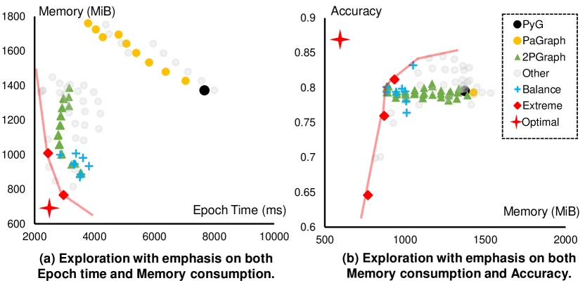
Figure 6. Adaptability validation of generated guidelines on Reddit2+SAGE.

4.3. Impact of Application Adaption

The trade-offs among three performance metrics are reported in Fig. 6. The performance statistics are collected by actually executing the training under different configuration settings from the design space. Design space has been exhausted and each point in Fig. 6 denotes the performance of a certain candidate in design space. Furthermore, we manually draw the Pareto front in red lines. The ground-truth performance of extreme (Ex) is marked with red color, and the ones of balance (Bal) are marked with blue color. The adaptability of GNNavigator can be validated since the provided guidelines can perfectly match the actual Pareto front.

Notably, the GNNavigator always takes approaches of existing works into consideration. Therefore, it will certainly recommend a reproduction of one existing approach as a guideline, if the approach just outperforms others under a given scenario.

4.4. Precision of Performance Estimator

Different evaluation metrics including R2 Score and Mean Square Error (MSE), are adopted to measure the precision of estimations in $T$, $\Gamma$, and $Acc$, according to their different methods of predicting. It is convinced that R2 Score is more suitable for models with relatively clear theoretical analysis, and MSE fits black-box models better. The results in Tab. 2 show that the ”gray-box” estimator can precisely foretell training performance in a low-latency way across a wide range of datasets. Bear in mind that R2 Scores indicate better precision of estimators when they are closer to 1. The R2 Scores of $T$ and $\Gamma$ range from 0.72 to 0.98, in terms of estimation on Reddit, Reddit2, and Ogbn-products. And MSE of $Acc$ estimation are controlled to a relatively low level, that is 0.03 in the worst case. These results strongly validate the effectiveness and correctness of our performance estimator.

Table 2. Validation of estimator prediction.

Prediction Validation	Performance Metric	Reddit	Reddit2	Ogbn-products
R2 Score	Time Cost ($T$)	0.8371	0.7328	0.7281
	Memory ($\Gamma$)	0.9240	0.9810	0.7307
MSE	Accuracy ($Acc$)	0.0292	0.0249	0.0156

5. Conclusions

We present GNNavigator, a GNN training framework with excellent adaptability to various application requirements. GNNavigator automatically generates training guidelines, consistently delivering promising performance across different scenarios. We draw unified abstractions from various optimizations and build a reconfigurable runtime backend based on the abstractions. To accurately predict training performance on our backend, we construct a gray-box performance estimator. GNNavigator further enables automatic exploration of training guidelines adapted to application requirements. Our experiments demonstrate that GNNavigator outperforms state-of-the-art works by up to 3.1$\times$ speedup and at most 44.9% reduction in memory consumption, with comparable accuracy.

References

- [1] Thomas N. Kipf and Max Welling. Semi-supervised classification with graph convolutional networks. In Proceedings of ICLR, 2017.
- [2] Petar Velickovic, Guillem Cucurull, Arantxa Casanova, Adriana Romero, Pietro Lio, Yoshua Bengio, et al. Graph attention networks. In Proceedings of ICLR, 2018.
- [3] Zhiqi Lin, Cheng Li, Youshan Miao, Yunxin Liu, and Yinlong Xu. Pagraph: Scaling gnn training on large graphs via computation-aware caching. In Proceedings of SoCC, 2020.
- [4] Tianfeng Liu, Yangrui Chen, Dan Li, Chuan Wu, Yibo Zhu, Jun He, Yanghua Peng, Hongzheng Chen, et al. BGL:GPU-efficient GNN training by optimizing graph data I/O and preprocessing. In Proceedings of NSDI, 2023.
- [5] Jie Chen, Tengfei Ma, and Cao Xiao. Fastgcn: Fast learning with graph convolutional networks via importance sampling. In Proceedings of ICLR, 2018.
- [6] Hanqing Zeng, Hongkuan Zhou, Ajitesh Srivastava, Rajgopal Kannan, and Viktor Prasanna. GraphSAINT: Graph sampling based inductive learning method. In Proceedings of ICLR, 2019.
- [7] Xin Liu, Mingyu Yan, Shuhan Song, Zhengyang Lv, Wenming Li, Guangyu Sun, et al. GNNSampler: Bridging the gap between sampling algorithms of gnn and hardware. In Proceedings of ECML PKDD, 2022.
- [8] Zhaodong Chen, Mingyu Yan, Maohua Zhu, Lei Deng, Guoqi Li, Shuangchen Li, and Yuan Xie. FuseGNN: Accelerating graph convolutional neural network training on GPGPU. In Proceedings of ICCAD, 2020.
- [9] Yuke Wang, Boyuan Feng, Gushu Li, Shuangchen Li, Lei Deng, Yuan Xie, and Yufei Ding. GNNAdvisor: An adaptive and efficient runtime system for GNN acceleration on GPUs. In Proceedings of OSDI, 2021.
- [10] Haoran You, Tong Geng, Yongan Zhang, Ang Li, and Yingyan Lin. GCOD: Graph convolutional network acceleration via dedicated algorithm and accelerator co-design. In Proceedings of HPCA, 2022.
- [11] Tim Kaler, Nickolas Stathas, Anne Ouyang, Alexandros-Stavros Iliopoulos, Tao Schardl, et al. Accelerating training and inference of graph neural networks with fast sampling and pipelining. Machine Learning and Systems, 2022.
- [12] Jianbang Yang, Dahai Tang, Xiaoniu Song, Lei Wang, Qiang Yin, Rong Chen, Wenyuan Yu, and Jingren Zhou. GNNLab: a factored system for sample-based GNN training over GPUs. In Proceedings of EuroSys, 2022.
- [13] Zirui Liu, Kaixiong Zhou, Fan Yang, Li Li, Rui Chen, and Xia Hu. EXACT: Scalable graph neural networks training via extreme activation compression. In Proceedings of ICLR, 2021.
- [14] Lizhi Zhang et al. 2PGraph: Accelerating GNN training over large graphs on GPU clusters. In Proceedings of CLUSTER, 2021.
- [15] Yingjie Qi, Jianlei Yang, Ao Zhou, Tong Qiao, and Chunming Hu. Architectural implications of GNN aggregation programming abstractions. IEEE CAL, 2023.
- [16] Matthias Fey and Jan Eric Lenssen. Fast graph representation learning with PyTorch Geometric. In Proceedings of ICLR, 2019.
- [17] Minjie Wang, Da Zheng, Zihao Ye, Quan Gan, Mufei Li, Xiang Song, et al. Deep graph library: A graph-centric, highly-performant package for graph neural networks. arXiv preprint arXiv:1909.01315, 2019.
- [18] Rong Zhu et al. AliGraph: A comprehensive graph neural network platform. arXiv preprint arXiv:1902.08730, 2019.
- [19] Yi-Chien Lin, Bingyi Zhang, and Viktor Prasanna. HitGNN: High-throughput GNN training framework on CPU+ multi-FPGA heterogeneous platform. arXiv preprint arXiv:2303.01568, 2023.
- [20] Yi-Chien Lin, Bingyi Zhang, and Viktor Prasanna. HP-GNN: Generating high throughput GNN training implementation on CPU-FPGA heterogeneous platform. In Proceedings of FPGA, 2022.
- [21] Ao Zhou, Jianlei Yang, Yingjie Qi, Yumeng Shi, Tong Qiao, Weisheng Zhao, and Chunming Hu. Hardware-aware graph neural network automated design for edge computing platforms. In Proceedings of DAC, 2023.
- [22] Chen Bai, Qi Sun, Jianwang Zhai, Yuzhe Ma, Bei Yu, and Martin DF Wong. BOOM-Explorer: RISC-V BOOM microarchitecture design space exploration rramework. In Proceedings of ICCAD, 2021.
- [23] Weihua Hu, Matthias Fey, Marinka Zitnik, Yuxiao Dong, Hongyu Ren, Bowen Liu, Michele Catasta, and Jure Leskovec. Open graph benchmark: Datasets for machine learning on graphs. arXiv preprint arXiv:2005.00687, 2020.
- [24] Adam Paszke et al. PyTorch: An imperative style, high-performance deep learning library. In Proceedings of NIPS, 2019.