Beyond Noise: Privacy-Preserving Decentralized Learning with Virtual Nodes

Abstract

DL enables collaborative learning without a server and without training data leaving the users’ devices. However, the models shared in DL can still be used to infer training data. Conventional privacy defenses such as differential privacy and secure aggregation fall short in effectively safeguarding user privacy in decentralized learning (DL). We introduce Shatter, a novel DL approach in which nodes create virtual nodes to disseminate chunks of their full model on their behalf. This enhances privacy by (i) preventing attackers from collecting full models from other nodes, and (ii) hiding the identity of the original node that produced a given model chunk. We theoretically prove the convergence of Shatter and provide a formal analysis demonstrating how Shatter reduces the efficacy of attacks compared to when exchanging full models between participating nodes. We evaluate the convergence and attack resilience of Shatter with existing DL algorithms, with heterogeneous datasets, and against three standard privacy attacks, including gradient inversion. Our evaluation shows that Shatter not only renders these privacy attacks infeasible when each node operates 16 VNs but also exhibits a positive impact on model convergence compared to standard DL. This enhanced privacy comes with a manageable increase in communication volume.

1 Introduction

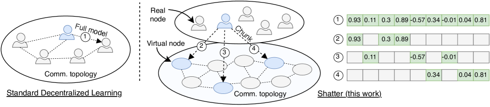
Figure 1: With standard decentralized learning (DL) (left), nodes continuously send their full model to other nodes in the communication topology. With Shatter, nodes operate multiple VNs (middle) and VNs directly communicate with other VNs. In addition, each VN sends a part of the full model of the RN to other VNs (right). This hides the identity of the original node that produced a given model chunk. The communication topology in Shatter changes every round to protect privacy further.

DL allows nodes to collaboratively train a global machine learning (ML) model without sharing their private datasets with other entities [40]. The nodes in DL are connected to other nodes, called neighbors, via a communication topology. DL is an iterative process where, in each round, nodes start with their local models and perform training steps on their private datasets. These updated local models are exchanged with neighbors in the communication graph and aggregated. The aggregated model is then used as the starting point for the next round, and the process repeats until model convergence is reached. Popular DL algorithms include D-PSGD [40], GL [50], and EL [10].

In DL, the private data of the participating nodes does not leave their devices at any point during the training process. While this is a major argument in favor of the privacy of DL solutions, recent works have shown that model updates being shared in DL networks can be prone to privacy breaches [9, 51]. For example, (i) membership inference attacks[56]allow attackers to infer if a particular data sample was used during training by a node, (ii) attribute inference attacks[66, 38]allow the inference of a particular attribute of the node from the model updates (, gender), and (iii) gradient inversion attacks[22, 77]allow the attackers to reconstruct private data samples used for training. These privacy violations form a significant barrier to adopting DL algorithms in application domains where user privacy is crucial, , healthcare or finance. While numerous privacy defenses have been proposed in centralized ML settings [39], there is a lack of adequate defenses against privacy attacks in DL. For instance, noise-based solutions bring privacy at the cost of convergence [71, 6], and secure aggregation schemes provide masking at the cost of high system complexity and communication overhead [71, 4, 31].

To address the privacy concerns of DL, we introduce Shatter, a novel DL system that protects the shared model updates from these privacy attacks. The key idea behind Shatter is to allow nodes to have direct access only to a model chunk, , a subset of all parameters rather than receiving the full model. Shatter achieves this by having each node operate multiple virtual nodes (VNs) that communicate model chunks with other VNs. The communication topology is randomized each round for better mixing and privacy protection of model chunks. This approach (i) hides the identity of the original node as only VNs are connected in the communication topology, and (ii) significantly raises the bar against privacy attacks on model chunks or a combination of model chunks from different nodes since an attacker has access to less information about a particular node [77, 55, 38].

We visualize the overall architecture of Shatter in Figure 1. Standard DL algorithms (left) connect nodes directly in a static communication topology, and nodes exchange their full model with neighbors every round. In Shatter (right), each node, which we refer to as a real nodes (RNs) in the context of Shatter, starts by creating some virtual nodes for itself. All the virtual nodes then participate in the communication topology construction. In Shatter, RNs perform the training and chunking of the models. Then VNs are responsible for disseminating model chunks through the communication topology. The right part of Figure 1 highlights how different VNs send different model chunks, where grayed-out chunks are not sent. Finally, model chunks received by VNs are forwarded back to their corresponding RN and aggregated there. The next round is then initiated, which repeats until the model converges.

We conduct a comprehensive theoretical analysis to formally prove the convergence of Shatter and theoretically demonstrate its privacy guarantees. We also implement Shatter to empirically evaluate its robustness against an honest-but-curious attacker that mounts three standard attacks: the linkability, membership inference, and gradient inversion attack. Our experimental results show that Shatter provides significantly better privacy protection compared to baseline approaches while even improving convergence speed and attainable model accuracy, at the cost of a manageable increase in communication costs.

In summary, we make the following contributions:

• We introduce Shatter, a novel privacy-preserving DL algorithm where real nodes (RNs) operate multiple virtual nodes (VNs) and VNs share model chunks with each other (Sections 3 and 4).

• We prove convergence guarantees for Shatter under an arbitrary number of local training steps between each communication round. Our bounds involve regularity properties of local functions, the number of local steps, a parameter that depends on the number of virtual nodes per real node and the degree of random graphs sampled at each communication round (Section 5.1).

• We formally show that as the number of VNs increases, both the likelihood of sharing full models and the expected number of exchanged model parameters between the RNs decrease. This offers analytical insight into the diminishing efficacy of attacks exploiting shared model parameters or gradient updates (Section 5.2).

• We implement Shatter and empirically compare its privacy robustness against state-of-the-art baselines and three privacy-invasive attacks: the linkability attack (LA), MIA and GIA (Section 6). Our results show that Shatter improves model convergence and exhibits superior privacy defense against the evaluated privacy attacks while also showcasing higher model utility.

2 Background and Preliminaries

In this work, we consider a decentralized setting with a set of nodes $\mathcal{N}$ that seek to collaboratively learn an ML model. This is also known as collaborative machine learning (CML) [58, 51]. Each node $i\in\mathcal{N}$ has its private dataset $D_{i}$ to compute local model updates. The data of each node never leaves the device. The goal of the training process is to find the parameters of the model $\theta$ that perform well on the union of the local distributions $D=\cup_{i=1}^{n}D_{i}$ by minimizing the average loss function:

$$\min_{\theta}f(\theta)=\frac{1}{n}\sum_{i=1}^{n}\underbrace{\mathbb{E}_{\xi\sim D_{i}}[F_{i}(\theta,\xi)]}_{:=f_{i}(\theta)},$$ (1)

where $n=|\mathcal{N}|$, $f_{i}$ is the local objective function of node $i\in\mathcal{N}$, and $F_{i}(\theta,\xi)$ is the corresponding loss of the model $\theta$ on the sample $\xi\in D_{i}$.

2.1 Decentralized Learning

DL [49, 40, 2] is CML CML algorithm in which each node exchanges model updates with its neighbors through a communication topology $G$ (Figure 1 (left)). Among many DL variants, decentralized parallel stochastic gradient descent (D-PSGD) [40, 34] is considered a standard algorithm to solve the DL training tasks (Algorithm 1). In a round $t\leq T$, each node $i$ executes $E$ local training steps of stochastic gradient descent (SGD) by sampling mini-batches from local distribution $D_{i}$ (Lines 1–1). Subsequently, it shares the updated model $\theta_{i}^{t}$ with its neighbors in the communication topology $G$ (Line 1). Finally, the node aggregates the models it received from its neighbors in $G$ by performing a weighted average of its local model with those of its neighbors (Line 1). Node $i$ then adopts the final $\theta_{i}^{T}$ (or any other intermediate model), thereby terminating the DL training round.

Epidemic Learning ( epidemic learning (EL)). The communication topology $G$ in standard DL remains unchanged throughout model training. It is proven that the convergence of particular static communication topologies is sub-optimal compared to dynamic topologies. This happens because a model update produced by a particular node might take many rounds to propagate across the network [2, 68]. This is the key idea behind epidemic learning (EL), a DL approach in which the communication graph is randomized at the beginning of each round (Lines 1–1 in Algorithm 1). It has been theoretically and empirically shown that this results in better mixing of ML models and therefore faster and better model convergence [10]. While EL leverages randomized topologies for better model convergence, we leverage this technique for increased privacy protection during DL model training.

1 Initialize $\theta_{i}^{(0)}$

2 for $t=1,\dots,T$ do

3       if doing EL then

4             Randomize communication topology $G$

5      for $e=1,\dots,E$ do

6             $\xi_{i}\leftarrow$ mini-batch of samples from $D_{i}$

7             $\theta_{i}^{(t)}\leftarrow\theta_{i}^{(t-1)}-\eta\nabla f_{i}(\theta_{i}^{(t-1)},\xi_{i})$

8            

9       Send $\theta_{i}^{(t)}$ to the neighbors in topology $G$

10       Aggregate models received from neighbors

11      

12return $\theta_{i}^{(T)}$

Algorithm 1 The D-PSGD and EL procedure, from the perspective of node $i$.

2.2 Privacy Attacks in CML

A key property of CML algorithms is that training data never leaves the node’s device, therefore providing some form of data privacy. The most notable CML approach is federated learning (FL), which uses a parameter server to coordinate the learning process [44]. Nonetheless, an adversarial server or nodes may be able to extract sensitive information from the model updates being shared with them. We next outline three prominent privacy attacks in CML.

Membership Inference Attack (MIA). The goal of the MIA is to correctly decide whether a particular sample has been part of the training set of a particular node [30]. This is broadly a black-box attack on the model, with the adversary having access to the global training set and samples from the test set, which are never part of the training set of any node. While we assume that the adversary can access actual samples from the global training and test set, this can be relaxed by generating shadow datasets [56]. Many MIA attacks are based on the observation that samples included in model training exhibit relatively low loss values as opposed to samples the model has never seen. Since the MIA can present a major privacy breach in domains where sensitive information is used for model training, this attack is widely considered a standard benchmark to audit the privacy of ML models [65]. Moreover, MIA is considered a broad class of the AIA [51, 74]. Since the MIA is more prevalent in literature, we focus in this work on the MIA.

We evaluate the privacy guarantees of Shatter using a loss-based MIA, mainly because of its simplicity, generality, and effectiveness [51]. The adversary queries the received model to obtain the loss values on the data samples. The negative of the loss values can be considered as confidence scores, where the adversary can use a threshold to output MIA predictions [66]. To quantify the attack regardless of the threshold, it is common to use the ROC-AUC metric on the confidence scores [43, 53]. More specifically, membership prediction is positive if the confidence score exceeds a threshold value $\tau$ and negative otherwise. Hence, we can compute the corresponding true positive rate (TPR) and false positive rate (FPR) for a given $\tau$. Intuitively, our objective is to maximize TPR (, the correct identification of members) while minimizing FPR (, the number of incorrect guesses).

Gradient Inversion Attack (GIA). With GIA, the adversary aims to reconstruct input data samples from the gradients exchanged during the training process in CML [77, 22]. This is a key privacy violation in contexts involving sensitive information, such as personal photographs, medical records, or financial information. Since the success of this attack depends on the information contained in the gradients, this white-box attack in DL is performed at the first communication round or convergence, when the gradient approximation by the adversary is the best [51]. GIA is an optimization problem where the adversary performs iterative gradient descent to find the input data that results in the input gradients [77, 12]. More sophisticated GIAs on image data include GradInversion [67] when the training is done on a batch of images, and ROG [71] using a fraction of gradients [71]. We use the state-of-the-art GIA scheme ROG to evaluate Shatter. In addition, we leverage artifacts and pre-trained weights of reconstruction networks provided with ROG and assume that the adversary knows the ground-truth labels of samples in the batch. These, however, can also be analytically obtained from the gradients of the final neural network layer [75, 61].

Linkability Attack (LA). In the context of obfuscated model updates, LA allows an adversary to link a received obfuscated update with the training set it came from [38]. Similar to the MIA, this is a loss-based black-box attack on the model, but contrary to MIA, the adversary has access to the training sets of each participating node. Similar to MIA, LA may be performed on shadow data representing the training sets of participating nodes instead of actual data. For simplicity, we assume the adversary can access the actual training sets. In this paper, an adversary performs LA on received model updates by computing the loss of each received model update on each available training set and reporting the training set with the lowest loss. When the obfuscated update does not contain the complete model update vector, , when using model sparsification, the adversary completes the vector with the averaged updates from the previous round, leading to the best results [38].

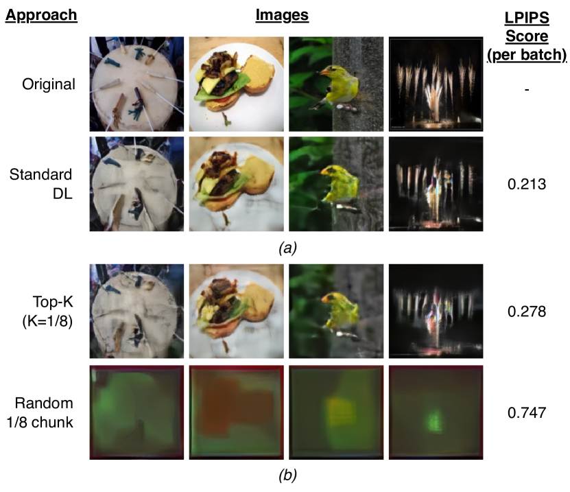
Figure 2: Selected reconstructed images (per row) using the GIA and the LPIPS score per batch, when using standard DL (a), TopK sparsification and random model chunking (b).

3 Shatter Motivation and Design Principles

The design of Shatter is anchored in three pivotal insights into the privacy challenges faced by conventional DL systems. We elaborate on these insights next.

1) Naive Model Sharing in DL Reveals Sensitive Data. A key aspect of collaborative ML mechanisms is that private data never leaves the devices of participating users. While this might give a sense of security, the work of Pasquini recently demonstrated how model sharing in standard DL settings can reveal sensitive information [51]. To show this empirically, we mark a single node as adversarial in a standard DL setting. During the first training round, this node conducts a GIA on the incoming models. Conducting the GIA during the first training round (or close to convergence) is optimal for the attack’s success. This is because it enables the adversary to reliably estimate the gradients during the first training round since all nodes in standard DL settings often start from a common model [51]. Each node trains its local model (LeNet) using a batch with $16$ images from ImageNet, and the adversary attempts to reconstruct the images in this batch using ROG [11]. Further details on the experiment setup are provided in in Section 6.1.

The results for four images are shown in Figure 2a, with the original image in the top row and the reconstructed image by the attacker with ROG and in DL in the second row. For each approach, we also show the associated LPIPS score of the reconstructed image [72]. This score indicates the perceptual image patch similarity, where higher scores indicate more differences between the original and reconstructed image batches. We observe significant similarities between the original and reconstructed images in DL settings, making it trivial for an attacker to obtain knowledge and semantics of private training data of other users. We verified that this also holds for the other images in the batch. The empirical findings highlighted by other DL studies [51] and our experiments illustrate that naive model sharing in DL falls short as a method for safeguarding data privacy: revealing sensitive data even in the early training rounds.

2) Sparsification to Protect Privacy. Sparsification in the context of collaborative ML is a technique aimed at reducing the communication overhead by selectively transmitting only a subset of model parameters or gradients during the training process [55, 59, 1, 42, 35, 33]. Instead of sharing the complete set of updates generated from local data, nodes or devices only send a fraction of the model updates, typically those with the highest magnitudes (Top-K sparsification) or chosen randomly (random sparsification). This approach can significantly decrease the amount of data exchanged between nodes or between nodes and a central aggregator. Furthermore, studies have suggested that it reduces the risk of privacy leaks as less information is shared among participants [64, 55, 77].

While the work of Yue demonstrates how TopK sparsification gives a false sense of privacy [71], there are key differences in privacy guarantees between standard sparsification techniques. Figure 2b shows the reconstructed images with ROG when the network uses TopK sparsification with $\frac{1}{8}$th of the model updates being communicated. Even though the LPIPS score related to using TopK sparsification is higher than when not using any sparsification (second row in Figure 2a), it is evident that TopK sparsification still allows an attacker to reconstruct potentially sensitive information from private training datasets. The bottom row in Figure 2b shows the reconstructed images by an adversary when each node randomly sends $\frac{1}{8}$th of its model update to neighboring nodes (random sparsification). While the TopK results follow the results of Yue  [71], random sparsification yields blurry images, making it nearly impossible for an adversary to obtain semantic information. This is also demonstrated by the associated LPIPS score, which is nearly three times as high as when using TopK sparsification. While it is evident that sparsification with random parameter selection is effective at obfuscating gradients in DL, sparsification has been shown to hurt time-to-convergence and final achieved accuracy, therefore prolonging the overall training process [28, 16, 15].

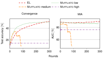
Figure 3: The test accuracy ($\uparrow$ is better) on the left and MIA attack success ($\downarrow$ is more private) on the right for EL and Muffliato with three noise levels, using CIFAR-10 as training dataset are presented here.

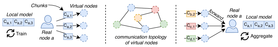
Figure 4: The three-step workflow of Shatter, showing the operations during a single training round. A RN $i$ first splits its local model into $k$ chunks and sends each chunk to one of its VNs (left). We refer to the $i$th chunk of RN $a$ as $C_{a,i}$. VN are connected into a communication topology and exchange model chunks with other VNs (middle). VN forward received chunks to the corresponding RN who aggregates the received chunks into its local model and performs a training step (right).

3) The Pitfalls of Noise-based Solutions. Another approach to increase privacy in CML is to add small perturbations (a.k.a. noise) to model updates before sharing them with other nodes [63, 70]. Noise-based mechanisms for DL with differential-privacy foundations like Muffliato [9] have been theoretically proven to converge while providing strong privacy guarantees. In practice, though, adding noise for privacy protection can hurt the utility of the model [71, 51]. We illustrate this by evaluating the convergence and the success of the membership-inference attack for both EL (DL variant) and Muffliato on a non independent and identically distributed (non-IID) partitioning of CIFAR-10 with ResNet-18. We comprehensively search for three noise levels for Muffliato, one with an attack success close to EL, one with a low attack success rate, and one in between. We run Muffliato with $10$ communication rounds as recommended by the authors of Muffliato [9]. While this increases the communication cost of Muffliato by $10\times$ compared to EL, we consider this fair from a convergence and privacy perspective.

Figure 3 shows our results and demonstrates the pitfalls of the state-of-the-art noise-based DL solution Muffliato. The figure shows the test accuracy and MIA attack resilience for EL and Muffliato for three different noise levels (low: $\sigma=0.025$, medium: $\sigma=0.05$, high: $\sigma=0.1$). While Muffliato (low) does reduce the MIA success rate when compared to EL, this reduction is marginal. The better convergence of Muffliato (low) can be attributed to the $10$ communication rounds in Muffliato as opposed to $1$ in EL that enable nodes to better aggregate the models across the network. We also observe that model training with Muffliato (medium) breaks down after roughly $45$ rounds into training. This is because noise introduces instability in the learning process, leading to nan loss values. On the other hand, Muffliato (high) handicaps the model utility as there is no convergence as shown in Figure 3 (left) and hence, the MIA is not representative of the learning process. We emphasize that there is no way to predict the noise levels in Muffliato and similar solutions that limit the adverse effect on convergence while reducing the success of privacy attacks. Furthermore, Yue empirically show that noise-based solutions hurts the final accuracy when reducing the success of GIA [71]. The results in Figure 3 highlight the need for practical privacy-preserving solutions that do not adversely affect the convergence of DL tasks.

4 Design of Shatter

Based on the findings in Section 3, we present the design and workflow of Shatter. The essence of Shatter is to exchange a randomly selected subset of parameters rather than the entire set (random sparsification) while still disseminating all the parameters through the network to not lose convergence. Shatter achieves this by having each RN operate multiple VNs and the VNs communicate random model chunks with other VNs. This enhances privacy as it significantly complicates the task of adversarial RNs to extract sensitive information from received model chunks.

4.1 System and Threat Model

Network.

Each VN has a unique identifier that identifies the node in the network. We assume a permissioned network in which nodes remain online and connected during model training, a standard assumption of many DL approaches. We consider threats at the network layers, such as the Eclipse and Sybil attacks [57, 17], beyond the scope of this work.

Each node can exchange messages with its neighbors through a communication topology represented as an undirected graph $G=(V,E)$, where $V$ denotes the set of all nodes and $(i,j)\in E$ denotes an edge or communication channel between nodes $i$ and $j$. Shatter connects VNs using a $r$-regular communication graph, which is a commonly used topology across DL algorithms due to its simplicity and load balancing. With this topology, each node has exactly $r$ incoming and outgoing edges, , sends and receives $r$ model chunks. The convergence of DL on $r$-regular graphs has extensively been studied [10]. In Shatter, the communication topology changes every training round, which can be achieved by having VNs participate in topology construction using a decentralized peer-sampling service [60, 32, 48]. In this paper, we stick to the EL-Oracle model [10] in which a central coordinator agnostic of the identities of RNs creates a random $r$-regular topology of only VNs every training round. We assume that nodes faithfully participate in the construction of the communication topology, which can be achieved by using accountable peer sampling services [69]. We consider the security and specifications of topology construction beyond the scope of this work.

Threat Model. We consider the RNs to be honest-but-curious, the participating RNs adhere to the working of the protocol but attempt to retrieve sensitive information about the other RNs from the model updates (chunks) it receives through its VNs. We do not consider any potential collusion between the real or the virtual nodes and assume that every VN works in the best interest of their corresponding RNs. On that note, we consider that the RNs have full control over their respective VNs in a sense that: $i)$ every RN may know which other VNs its own VNs have communicated with in a given training round, and $ii)$ the information about which parent RN controls a given VN cannot be retrieved by any other VN or RN (the link between any RN and its corresponding VNs is hidden from everyone else in the network). An attacker may store historical model updates or other information it has received and act on this. Attacks targeted at the network layer, , attempting to link a RN and its VNs through network inspection, are considered beyond the scope of this work.

4.2 Shatter Workflow

We show the full workflow of Shatter in Figure 4 and provide pseudocode in Algorithm 2. In Shatter, each participating real node (RN) creates a set of $k$ VNs for itself (Line 2). To streamline our analysis, we work under the assumption that each RN operates the same number of VNs. We show in Section 5.2 that increasing $k$, , spawning more VNs, reduces the vulnerability against privacy attacks. We refer to a RN $a$ as the parent RN of a VN $v$ if $v$ was spawned by $a$. These VNs are, in practice, implemented as processes on remote systems.

At the start of each training round, a RN first updates its local model using its private dataset (Lines 2–2). VNs then refresh the communication topology $G$. The RN then segregates its local model into $k$ smaller model chunks (specifications are given later) and forwards these to its VNs that multicast the model on the RN’s behalf (Line 2). We also visualize this in Figure 4 (left) where some real node $a$ segregates its local model into three chunks $C_{a,1},C_{a,2}$ and $C_{a,3}$, each of which is forwarded to a VN of $a$. In Shatter, VNs thus act as communication proxy for model chunks created by RNs. All model chunks received by a VN during a training round are forwarded back to its parent RN and aggregated into the local model (Algorithm 2). This is also visualized in Figure 4 (right) where a RN $a$ receives model chunks from VNs operated by RNs $b,c$ and $d$. We note that $a$ is oblivious to the identity of the RN behind the received model chunks. In essence, from the perspective of a single node, it sends out the same number of model parameters as in standard DL. The node sends a smaller subset of random parameters to one node but sends these to more nodes, which helps privacy without adverse effects on convergence.

1 Initialize $\theta_{i}^{(0)}$

2 Spawn $k$ virtual nodes (VNs)

3 for $t=1,\dots,T$ do

4       for $e=1,\dots,E$ do

5             $\xi_{i}\leftarrow$ mini-batch of samples from $D_{i}$

6             $\theta_{i}^{(t)}\leftarrow\theta_{i}^{(t-1)}-\eta\nabla f_{i}(\theta_{i}^{(t-1)},\xi_{i})$

7            

8       Randomize communication topology $G$

9       Chunk $\theta_{i}^{(t)}$ into $s$ chunks

10       for $s=1,\dots,k$ do

11            Forward chunk $s$ to $v_{i}(s)$

12            

13      Aggregate $kr$ chunks received from VNs

14      

15return $\theta_{i}^{(T)}$

Algorithm 2 Shatter from the perspective of RN $i$

Dynamic Topologies. In standard DL algorithms, RNs directly communicate their model updates. Shatter instead connects VNs in a communication topology $G$, also see Figure 4 (middle). $G$ is refreshed every training round to enhance privacy. The benefits of dynamic topologies over static topologies in Shatter are twofold. Firstly, it restricts any attacker from receiving model chunks consistently from a VN of the same victim node. This reduces the chances of attacks that target specific nodes as an attacker is unable to reliably obtain model chunks from the victim across training rounds. Secondly, dynamic topologies converge faster than static ones thanks to the better mixing of the models [10].

Compared to standard DL approaches such as EL, Shatter has a marginal increase in communication cost. We derive in Appendix A that the communication cost of Shatter increases by a factor $2+\frac{1}{r}$ compared to EL, where $r$ is the degree of the topology. This corresponds to a $2-3\times$ increase in communication.

Model Aggregation. In Shatter, a RN may receive a parameter at the same index in the model multiple times or not receive a particular parameter at all. Shatter uses a parameter-wise weighted averaging where the parameter is proportional to the frequency of how often this parameter is received. For example, if a parameter $p$ is received two times, $p_{1}$ and $p_{2}$ referring to these individual parameters, a RN will average $p_{1}$, $p_{2}$ and the same parameter in its local model while using an averaging weight of $\frac{1}{3}$ for each parameter. We remark that each RN receives the same total number of parameters, but the count of incoming parameters at a particular index may differ.

4.3 Model Chunking Strategy

RNs in Shatter break down their local model into smaller chunks that are propagated by their VNs. The strategy for model chunking can affect both the convergence of the training process and the privacy guarantees. We discuss three model chunking strategies and analyze their trade-offs in terms of convergence and privacy.

1) Linear Chunking. With linear chunking, the model parameters are flattened to a one-dimensional array of weights and linearly partitioned into $k$ chunks. Thus, the first $\frac{1}{k}$ parameters are given to the first VN, the next $\frac{1}{k}$ parameters to the second VN etc. However, we experimentally found this strategy to violate privacy since different model chunks carry different amounts of information since they contain information from different layers. For example, the last chunk containing the weights associated with the final layer can leak substantial gradient information [75, 61].

2) Random Weight Sampling (with replacement). Another strategy involves a RN sampling $\frac{1}{k}$ random weights, with replacement. However, this strategy risks an adversarial RN inferring that two model chunks originate from the same RN. Specifically, a RN receiving two model chunks that share a common weight at the same position can now, with a high likelihood, conclude that those chunks originate from the local model of the same RN.

3) Random Weight Sampling (without replacement). Another strategy involves continuously sampling weights from the local model, without replacement. This does not suffer from the privacy concern associated with sampling with replacement since the weight indices in two chunks from the same RN will always be disjoint. Another advantage of this strategy is that each parameter will be chosen in a round.

In Shatter, we adopt the random weight sampling (without replacement) strategy. Furthermore, we use static model chunking where a RN will create chunks with the same indices across different training rounds. This prevents RNs from inferring that two received model chunks across rounds originate from the same RN, potentially close to convergence.

5 Theoretical Analysis

Notations.

Let $\mathcal{N}=\{N_{1},\ldots,N_{n}\}$ be the RNs in the network. Setting $d\in\mathbb{N}$ as the dimension of the parameter space, let $\theta^{(t)}_{i}=\left(\theta^{(t)}_{i}(1),\ldots,\theta^{(t)}_{i}(d)\right)\in\mathbb{R}^{d}$ be the model held by $N_{i}$ in the $t^{\operatorname{th}}$ communication round for every $i\in[n]$. Letting each RN have $k$ VNs with $v_{i}(s)$ denoting the $s^{\operatorname{th}}$ VN of $N_{i}$ for all $i\in[n]$ and $s\in[k]$, let $\theta_{i,s}^{(t)}$ be the chunk of $N_{i}$’s model that is forwarded to $v_{i}(s)$ in round $t$. For every $i,j\in[n]$ and $p\in[d]$, let $\theta_{i\leftarrow j}^{(t)}(p)$ denote the $p^{\operatorname{th}}$ parameter of $N_{j}$’s model that is shared with $N_{i}$ and, correspondingly, let $\theta^{(t)}_{i\leftarrow j}=\left(\theta_{i\leftarrow j}^{(t)}(1),\ldots,\theta_{i\leftarrow j}^{(t)}(d)\right)$ be the entire contribution that $N_{i}$ receives from $N_{j}$’s model updates (via the communication of their VNs) for aggregation leading up to the next communication round.

In the subsequent analysis, we shall assume that:

1. the number of model parameters held by each VN is the same (i.e., $d=kc$ for some $c\in\mathbb{N}$ and the chunks of the models assigned to each VN partitions the model of the corresponding RN into $k$ equal sizes of $c$).

2. the $kn$ total VNs collectively form an $r$-regular dynamic topology, for some $1\leq r\leq nk-1$, facilitating interaction among them for the exchange of the model chunks they individually hold.

5.1 Convergence of Shatter

We now study the convergence properties of the decentralized algorithm we use for our training. For $i\in[n]$, let $f_{i}:\mathbb{R}^{d}\to\mathbb{R}$ be the loss of node $N_{i}$ with respect to its own dataset, and let $f=\frac{1}{n}\sum_{i=1}^{n}f_{i}$ the function that nodes seek at minimizing. Nodes will alternate between rounds of $H\geq 1$ local stochastic gradient steps and communication rounds, that consist of communications through virtual nodes.

For the $t^{th}$ communication round, let $\mathcal{G}_{t}=(\mathcal{V},\mathcal{E}_{t})$ be the graph on the virtual nodes, where $\mathcal{V}=\{v_{i}(s),i\in[n],s\in[k]\}$ is the set of virtual nodes, and $\mathcal{E}_{t}$ is the set of edges of $\mathcal{G}_{t}$, a graph sampled uniformly at random and independently from the past in the set of $r$-regular graphs on $\mathcal{V}$. A communication round consists of a simple gossip averaging in the Virtual Nodes graph: this could be refined with accelerated gossip averaging steps [19] or compressed communications [35] for instance. Note that for computation steps, no random noise is added, as opposed to other decentralized privacy-preserving approaches, such as [9] for gossip averagings or [8, 18] for token algorithms. As for communications, computations are also assumed to be synchronous, and leveraging asynchronous local steps such as asynchronous SGD steps in the analysis would require more work [46, 76].

We now can write the updates of the training algorithm as follows.

1. Local steps. For all $i\in[n]$, let $\tilde{\theta}_{i}^{(t,0)}=\theta_{i}^{(t)}$ and for $h\leq H-1$,

   $$\tilde{\theta}_{i}^{(t,h+1)}=\tilde{\theta}_{i}^{(t,h)}-\eta g_{i}^{(t,h)}\,,$$

   where $\eta>0$ is the learning-rate and $g_{i}^{(t,h)}$ a stochastic gradient of function $f_{i}$, sampled independently from the past.

2. Communication step. Let $\hat{\theta}_{i}^{(t)}=\theta_{i}^{(t,H)}$ and for a virtual node $v_{i}(s)$ let $\hat{\theta}_{v_{i}(s)}^{(t)}$ be its model chunk. Then, an averaging operation is performed on the graph of virtual nodes:

   $$\theta_{i}^{t+1}=\sum_{s=1}^{k}\frac{1}{r}\sum_{w\in\mathcal{V}:\{v_{i}(s),w\}\in\mathcal{E}_{t}}\hat{\theta}_{w}^{(t)}\,.$$

Lemma 1.

Let $\mathcal{C}_{t}:\mathbb{R}^{d\times n}\to\mathbb{R}^{d\times n}$ be the operator defined as

$$\forall\theta=(\theta_{i})_{i\in[n]}\in\mathbb{R}^{d\times n}\,,\quad\mathcal{C}_{t}(\theta)_{i}=\sum_{s=1}^{k}\frac{1}{r}\sum_{w\in\mathcal{V}:\{v_{i}(s),w\}\in\mathcal{E}_{t}}\theta_{w}\,,$$

where for $w=v_{i}(s)$ a virtual node of $N_{i}$, $\theta_{w}\in\mathbb{R}^{d}$ contains the subset of coordinates of $\theta_{i}$ associated to the model chunks of $v_{i}(s)$. We have, for all $\theta=(\theta_{i})_{i\in[n]}\in\mathbb{R}^{d\times n}$:

$$\frac{1}{n}\sum_{i=1}^{n}\mathcal{C}_{t}(\theta)_{i} =\bar{\theta}\,,$$ (2)

$$\mathbb{E}\left[\frac{1}{n}\sum_{i=1}^{n}\left\|\mathcal{C}_{t}(\theta)_{i}-\bar{\theta}\right\|^{2}\right] \leq\frac{\rho}{n}\sum_{i=1}^{n}\left\|\theta_{i}-\bar{\theta}\right\|^{2}\,,$$ (3)

where $\bar{\theta}=\frac{1}{n}\sum_{i=1}^{n}\theta_{i}$ and

$$\rho=\frac{nk}{r(nk-1)}\left(1+\frac{k-r}{nk-3}+\frac{(k-1)(r-1)}{(nk-2)(nk-3)}\right)\,.$$ (4)

The proof is postponed to Section C.3. Importantly, the inequality in Equation 3 for $\rho$ as in Equation 4 is almost tight, up to lower order terms in the expression of $\rho$.

Using this and adapting existing proofs for decentralized SGD with changing topologies and local updates [34, 20] we get the following convergence guarantees.

Theorem 2.

Assume that functions $f_{i}$ are $L-$smooth, $f$ is lower bounded and minimized at some $\theta^{\star}\in\mathbb{R}^{d}$, the stochastic gradients are unbiased ($\mathbb{E}g_{i}^{(t,h)}=\nabla f_{i}(\tilde{\theta}_{i}^{(t,h)})$ for all $i,t,h$), of variance upper bounded by $\sigma^{2}$:

$$\frac{1}{n}\sum_{i=1}^{n}\mathbb{E}\left[\left\|g_{i}^{(t,h)}-\nabla f_{i}(\tilde{\theta}_{i}^{(t,h)})\right\|^{2}\right]\leq\sigma^{2}\,,$$

and let $\zeta^{2}$ be the population variance, that satisfies:

$$\forall\theta\in\mathbb{R}^{d}\,,\quad\frac{1}{n}\sum_{i=1}^{n}\left\|\nabla f_{i}(\theta)-\nabla f(\theta)\right\|^{2}\leq\zeta^{2}\,.$$

Finally, assume that $\rho<1$. Then, for all $T>0$, there exists a constant stepsize $\eta>0$ such that:

$$\frac{1}{T}\sum_{t<T}\mathbb{E}\left[\left\|\nabla f(\bar{\theta}^{(t)})\right\|^{2}\right] =\mathcal{O}\left(\sqrt{\frac{LF_{0}\sigma^{2}}{nHT}}+\frac{LF_{0}}{T(1-\rho)}\right.$$

$$\quad\left.+\left[\frac{LF_{0}\big{(}H\zeta+\sigma\sqrt{(1-\rho)H}\big{)}}{(1-\rho)HT}\right]^{\frac{2}{3}}\right)\,,$$

where $F_{0}=f(\bar{\theta}^{(0)})-f(\theta^{\star})$.

The proof is postponed to Section C.4 The convergence bound shows that Shatter will find first-order stationary points of $f$: since $f$ is non-convex, we fall back to show that the algorithm will find an approximate first-order stationary point of the objective [7]. The first term $\sqrt{\frac{LF_{0}\sigma^{2}}{nHT}}$ is the largest as $T$ increases: it is the statistical rate: $nHT$ is exactly the number of stochastic gradients computed up to iteration $T$, and this term cannot be improved [7]. The second and third terms are then lower order terms: for $T=\Omega(nH(1-\rho)^{-2})$, the first term dominates.

Then, the assumption $\rho<1$ needs to be verified. As $n$ becomes large, it will always be satisfied for $r>1$: in the $n-$large regime, $\rho$ scales as $\rho\sim\frac{1}{r}$: increasing $r$ will always lead to faster communications. However, it appears that $\rho$ only needs to be bounded away from $1$, as only the $1/(1-\rho)$ factor appears in the rate. Having $\rho\leq 1/2$ is sufficient to obtain the best rates, and this only requires $r=\mathcal{O}(1)$: There is no need to scale $r$ with $n$, and the graph of virtual nodes can have bounded degrees.

5.2 Privacy Guarantees

Under the threat model that we consider (as delineated in Section 4.1), if $\theta^{(t)}_{i\leftarrow v_{i}(s)}(p)$ is the model parameter $p\in[d]$ that RN $N_{i}\in\mathcal{N}$ receives from its VN $v_{i}(s)$ for any $s\in[k]$ after any communication round $t$, we note that:

$$\mathbb{P}\left[\theta^{(t)}_{i\leftarrow v_{i}(s)}(p)=\theta^{(t)}_{i\leftarrow j}(p)\right]=\mathbb{P}\left[\theta^{(t)}_{i\leftarrow v_{i}(s)}(p)=\theta^{(t)}_{i\leftarrow j^{\prime}}(p)\right]$$

for every $j,j^{\prime}\in[n],\,j\neq j^{\prime}$. In other words, as the VNs that communicate with $v_{i}(s)$ do not reveal any information about their respective parent RNs, the model parameters transmitted by them to $v_{i}(s)$ (which, in turn, $N_{i}$ receives) are equiprobable to come from any of the other participating RNs. Hence, by achieving perfect indistinguishability among the RNs w.r.t. the model parameters received in any communication round, we analyze the probabilistic characteristics of the received model parameters to establish a fundamental understanding of how empirical risks are influenced in the face of attacks relying on shared model updates.

First, we aim to investigate the probability of a certain RN to obtain the entire model of a different RN that may, in turn, result in severe privacy loss and assist the relevant attacks exploiting the sharing of the full models (GIA). To this purpose, we define the notion of distance between the models of a pair of RNs.

Definition 5.1 (Distance between models).

Let $\sigma:\mathbb{R}\mapsto\{0,1\}$ denote the discrete metric, i.e., $\forall\,z,z^{\prime}\in\mathbb{R}$, we have:

$$\sigma(z,z^{\prime})=\begin{cases}0\text{, if $z=z^{\prime}$,}\\ 1\text{, otherwise.}\end{cases}$$

Then, for a pair of models $\theta,\theta^{\prime}\in\mathbb{R}^{d}$, let the distance between them be $\delta(\theta,\theta^{\prime})$ such that:

$$\delta(\theta,\theta^{\prime})=\sum\limits_{p=1}^{d}\sigma(\theta(p),\theta^{\prime}(p)).$$

Remark 1.

Definition 5.1 suggests that for a pair of RNs $N_{i},N_{j}$, in some round training $t$, if $N_{i}$ receives all the parameters of $N_{j}$’ model update (via communication between their corresponding VNs), then $\delta\left(\theta^{(t)}_{j},\theta^{(t)}_{i\leftarrow j}\right)=0$. In general, if if $N_{i}$ receives $0\leq d_{0}\leq d$ of the parameters of $N_{j}$’s model update, then $\delta\left(\theta^{(t)}_{j},\theta^{(t)}_{i\leftarrow j}\right)=d-d_{0}$.

Theorem 3.

For any $i,j\in[n]$, with $i\neq j$, and $t>0$:

$$\mathbb{P}\left[\delta\left(\theta^{(t)}_{j},\theta^{(t)}_{i\leftarrow j}\right)=0\right]$$

is a decreasing function of $k$.

Remark 2.

Theorem 3 essentially implies that under Shatter, the probability that all the model parameters of any RN being shared with another RN in any given communication round decreases with an increase in the number of VNs. The proof is postponed to Appendix C.1.

Theorem 4.

For any $i,j\in[n]$, with $i\neq j$, and $t>0$:

$$\mathbb{E}\left[\delta\left(\theta^{(t)}_{j},\theta^{(t)}_{i\leftarrow j}\right)\right]$$

is an increasing function of $k$.

Remark 3.

In essence, Theorem 4 ensures that under Shatter, the expected number of model parameters received by any RN from any other RN decreases (i.e., the expected distance between the shared models increases) with an increase in the number of VNs. See Section C.2 for the proof.

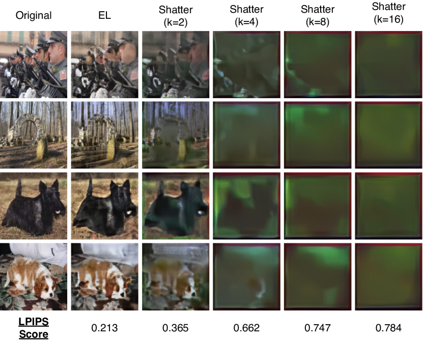
Figure 8: Selected reconstructed images using the GIA, for our baselines and different numbers of VNs ($k$). We also show the LPIPS scores for each setting at the bottom of the figure.

One of the important implications jointly posed by Theorem 3 and Theorem 4 is that with an increase in the number of VNs, $i)$ the chances of an attacker to receive the full model of any user, and $ii)$ the average number of model parameters exchanged between the RNs will both decrease. These, in turn, would make Shatter more resilient towards attacks that rely on exploiting the shared model parameters or gradient updates in their entirety. This provides an analytical insight into how Shatter effectively safeguards against the gradient inversion attack, as evidenced by the experimental results in Figure 8. The findings are aligned with the conclusions drawn from Theorem 3 and Theorem 4, indicating the diminished effectiveness of gradient inversion attacks with an increasing number of VNs.

6 Evaluation

Our evaluation answers the following questions:

1. How does the convergence and MIA resilience of Shatter evolve across training rounds, compared to our baselines (Section 6.2)?

2. How resilient is Shatter against the privacy attacks in DL (Section 6.3)?

3. How does increasing the number of VNs affect the model convergence and attack resilience (Section 6.4)?

6.1 Experimental Setup

Implementation and Compute Infrastructure. We implement Shatter using the DecentralizePy framework [15] in approximately $4300$ lines of Python 3.8.10 relying on PyTorch 2.1.1 [52] to train and implement ML models. Each node (RN and VN) is executed on a separate process, responsible for executing tasks independently of other nodes.

All our experiments are executed on AWS infrastructure, and our compute infrastructure consists of $25$ g5.2x large instances. Each instance is equipped with one NVIDIA A10G Tensor Core GPU and $8$ second-generation AMD EPYC 7R32 processors. Each instance hosts between 2-4 RNs and 1-16 VNs for each experiment.

DL algorithm and baselines. Shatter uses EL as the underlying learning algorithm (also see Section 2). As such, we compare the privacy guarantees offered by Shatter against those of EL, , in a setting without additional privacy protection. While many privacy-preserving mechanisms are designed for FL, only a few are compatible with DL. We use Muffliato as a baseline for privacy-preserving DL [9]. Muffliato is a noise-based privacy-amplification mechanism in which nodes inject local Gaussian noise into their model updates and then conduct $10$ gossiping rounds to average the model updates in each training round. For all experiments, unless otherwise stated, we set the number of VNs per RN $k=$ $8$ and generate a random regular graph with degree $r=$ $6$ every communication round.

Privacy Attacks. We evaluate Shatter against (i) Loss-based MIA, (ii) GIA, and (iii) LA. MIA is a representative inference attack, quantified using the negative of the loss values on the training samples of a node and the test set of the given dataset [66]. Since Shatter works with chunks of the model, LA measures how much a VN links to the training distribution [38] by evaluating each received model update and evaluating the loss on the training sets of each node. In both MIA and LA, the full model is required to compute the loss. Therefore, in Shatter, the adversary complements each chunk of the received model update with the average model of the previous round to approximate the full model before attacking it. GIA over the sparsified model updates is performed using the state-of-the-art ROG [71].

Learning Tasks and Hyperparameters. In our testbed, we use three datasets: CIFAR-10 [37], Twitter Sent-140 [5, 23], and MovieLens [26] for convergence, MIA, and LA. Additionally, we perform GIA (ROG) on a fraction of the images from the ImageNet [11] validation set.

The CIFAR-10 dataset is an image classification task that contains $50\,000$ training images and $10\,000$ test images. For CIFAR-10, we adopt a non-IID data partitioning scheme, assigning training images to $100$ DL nodes with a Dirichlet distribution. This is a common scheme to model data heterogeneity in CML [62, 25, 29, 10]. This distribution is parameterized by $\alpha$ that controls the level of non-IIDness (higher values of $\alpha$ result in evenly balanced data distributions). For all experiments with CIFAR-10, we use $\alpha=0.1$, which corresponds to a high non-IIDness. This simulates a setting where the convergence is slower in DL and the MIA and LA adversary have an advantage because the local distributions are dissimilar. Thus, we consider this an important setting to evaluate privacy-preserving mechanisms in DL. We use a ResNet-18 model [27] with approximately $11.5$ million trainable parameters.

Our second dataset is Twitter Sent-140, a sentiment classification task containing $1.6$ million tweets partitioned by users [23, 5]. We preprocess the dataset such that each user has at least $24$ tweets, resulting in a training set of $32\,299$ and a test set of $8484$ tweets. All tweets have been annotated with a score between 0 (negative) and 4 (positive). We randomly assign the different authors behind the tweets in the Twitter Sent-140 dataset to $50$ DL nodes, a partitioning scheme that is also used in related work on DL [16, 15]. For this task, we initialize a pre-trained bert-base-uncased language model from Hugging Face with a new final layer with $2$ outputs, which is based on the Transformer architecture and contains approximately $110$ million parameters [13]. We then fine-tune the full model on the Twitter Sent-140 dataset.

We also evaluate Shatter using a recommendation model based on matrix factorization [36] on the MovieLens 100K dataset, comprising user ratings from $0.5$ to $5$ for several movies. The dataset is partitioned into a training set comprising $70\,000$ samples and a test set comprising $30\,000$ samples. This task imitates a scenario where individual participants may wish to learn from the movie preferences of other users of similar interests. Like the Twitter Sent-140 learning task, we consider the multiple-user-one-node setup where we randomly assign multiple users to a DL node.

Lastly, to present the vulnerability of DL and Shatter towards GIA, we instantiate $2$ DL nodes, each with $16$ images from the ImageNet validation set. We use the LeNet model to perform one DL training round. ROG is performed on the model updates exchanged after the first training round. Since the reconstructed images are the best after the first training round, we do not continue further DL training.

We perform $1$ epoch of training before exchanging models for all convergence tasks and $5$ epochs of training for the ImageNet GIA. Learning rates were tuned on a grid of varying values. For Muffliato, we comprehensively use two noise levels: (i) low: with good convergence, which results in low-privacy against MIA, and (ii) high: with higher attack resilience to MIA, but at the cost of model utility. Lower noise values present no privacy benefits against EL, and higher noise values adversely affect convergence. More details about the hyperparameters can be found in Appendix B. In summary, our experimental setup covers datasets with differing tasks, data distributions, and model sizes, and the hyperparameters were carefully tuned.

Metrics and Reproducibility. All reported test accuracies are top-1 accuracies obtained when evaluating the model on the test datasets provided by each dataset. For MovieLens, we only present the RMSE-loss, as it is not a classification task. To quantify the attack resilience of Shatter and its baselines, we use the ROC-AUC metric when experimenting with the MIA, representing the area-under-curve when plotting the true positive rate against the false positive rate. For the LA, we report the success rate in percentage, , for each adversary, the success rate is computed as the percentage of correctly linked model chunks out of the total attacked model chunks. As the attacks are extremely computationally expensive, each RN across all baselines evaluates $8$ received model updates for CIFAR-10 and MovieLens, and $4$ for the Twitter Sent-140 dataset every training round. Finally, we report the LPIPS score when evaluating ROG, a score between 0 and 1, which indicates the similarity between two batches of images (more similar images correspond to lower LPIPS scores). We run all experiments three times, using different seeds, and present averaged results.

6.2 Convergence and MIA Across Rounds

We first evaluate how the convergence and resilience against the MIA evolve with the training for Shatter and the baselines for all three datasets. Each RN operates $8$ VNs, and we train until EL convergences. An ideal algorithm would have a low MIA AUC and a high test accuracy (or test loss for MovieLens) close to EL with no privacy-preserving solution.

Figure 5 shows the convergence (left) and MIA attack success (right) for each dataset (row-wise). EL achieves $51.74$%, $83.11$%, and $1.10$ [RMSE] model utility for CIFAR-10, Twitter Sent-140, and MovieLens, respectively. On the other hand, EL is vulnerable to the loss-based MIA, reaching close to $89.7$% AUC on CIFAR-10, $56.1$% AUC on Twitter, and $65.8$% AUC on MovieLens respectively, where the chance of a random guess is $50$%. Muffliato (low) achieves similar convergence to EL for all datasets but is also not very effective at reducing vulnerability against the MIA. Muffliato (high) instead lowers the MIA vulnerability but at the cost of convergence, finally reaching $2.61$% lower test accuracy for Twitter Sent-140, and $1.0$ [RMSE] higher test loss for MovieLens (considering the best values). For the CIFAR-10 dataset, convergence is so unstable that there is no learning beyond $12$ training rounds. In contrast, Shatter consistently outperforms the baselines in terms of the resilience to MIA while having no adverse impact on convergence for Twitter Sent-140 and MovieLens, and positively raises the top-1 test accuracy by $3.21$% for CIFAR-10. For a given iteration, Shatter reduces MIA AUC (%) by $4.9$-$25.8$% on CIFAR-10, $3.4$-$4.0$% on Twitter Sent-140, and $0.8$-$15.1$% on MovieLens.

These experiments cover a range of settings, , we find that the extreme non-IIDness in CIFAR-10 adversely affects Muffliato, whereas it positively affects Shatter. Furthermore, the pre-training in Twitter Sent-140 experiments makes it more challenging for the adversary to perform a MIA as models become less personalized. In CIFAR-10, Shatter has a higher vulnerability to MIA at the start, decreasing sharply afterward. We notice the accuracy of the models at this point is as good as a random guess ($10$%), and hence training techniques like regularization can fix it. However, we do not evaluate with regularization and show the worst case from the attack’s perspective. Another seemingly unexpected behavior is the higher vulnerability of Muffliato (high) against Muffliato (low). This can be explained by the loss curve on the left, which clearly shows significantly worse generalization for Muffliato (high) than Muffliato (low).

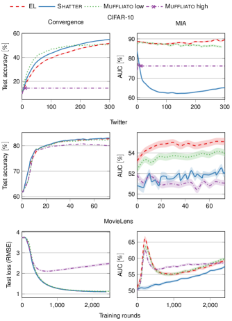
Figure 5: The test accuracy and MIA AUC ($\downarrow$ is better) across training rounds for CIFAR-10 (top), Twitter Sent-140 (middle) and MovieLens (bottom), for EL, Shatter and Muffliato. A MIA AUC of 50% corresponds to an attacker randomly guessing the membership of samples.

6.3 Privacy Guarantees of Individual Nodes

We now analyze the vulnerability of individual nodes to the MIA and LA. Ideally, we aim for most nodes to have a low MIA AUC and LA success. Figure 6 shows the CDF of victim nodes against the average MIA AUC (left) and LA success (right) for the baselines. We observe that, consistently across datasets, Shatter outperforms Muffliato (low) and EL in defending against both attacks. Muffliato (high) appears to beat Shatter on the Twitter Sent-140 dataset and appears to be a better defense against LA for CIFAR-10. However, we need to keep in mind that Muffliato (high) significantly hurts convergence (see Figure 5).

LA here also assesses the vulnerability of the real identities of the nodes that can be leaked through their local data distributions, even when the real identities and model updates are obfuscated. Shatter defends the privacy of the nodes by having near-zero linkability for at least $70$% across our experiments, up from only $7$% nodes with near-zero linkability in EL. Hence, Figure 6 (right) demonstrates that just obfuscating identities, , by using onion routing techniques [24], would not defend against LA. While Muffliato (high) is also decent in the defense against LA, this needs to be looked at in conjunction with the convergence. To conclude, Shatter offers individual clients better privacy protection compared to the baselines and across a range of varying learning tasks.

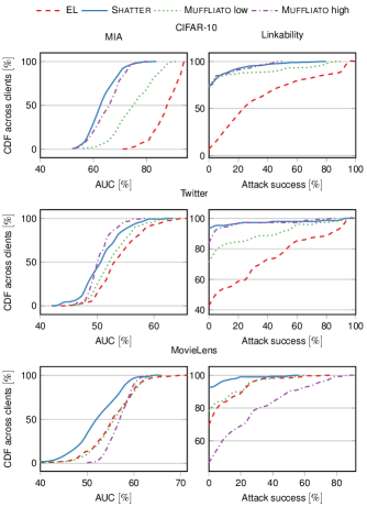
Figure 6: The distribution of MIA AUC ($\downarrow$ is better) and attack success of the LA across clients for CIFAR-10 (top), Twitter Sent-140 (middle) and MovieLens (bottom), for EL, Shatter and Muffliato. An attack success of 1% for the LA corresponds to an attacker randomly guessing.

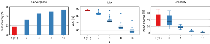
Figure 7: The test accuracy (left), MIA AUC (middle, $\downarrow$ is better) and attack success rate for LA (right), for CIFAR-10 and for increasing values of $k$. $k=1$ corresponds to an EL setting.

6.4 Varying the Number of VNs

We next analyze the impact of an increased number of VNs on convergence and resilience against our three privacy attacks.

Convergence. To observe the impact of $k$ on convergence, we run EL and Shatter with increasing values of $k$ for at most $300$ training rounds and with the CIFAR-10 dataset. The bar plot in Figure 7 (left) shows the highest observed average test accuracy during a run for different values of $k$. EL achieves an average test accuracy of 51.7%, which increases to 53.2% with $k=2$. Further increasing $k$ positively affects the test accuracy: increasing $k$ from $2$ to $16$ increases the attained test accuracy from 53.2% to 55.3%. We attribute this increase in test accuracy to the superior propagation and mixing of model chunks.

Attack Resilience. Next, we compare the attack resilience of Shatter with different values of $k$ against that of EL, for all three privacy attacks. The middle and right plot in Figure 7 shows the AUC and attack success percentage for the MIA and LA, respectively, for increasing values of $k$ and EL. The values for a fixed $k$ are averaged across clients and training rounds. Figure 7 (middle) shows that even $k=2$ already enhances privacy and reduces the median AUC from 88% to 83%. Shatter with $k=16$ provides significant privacy guarantees, showing a median AUC of just 0.58. A similar trend is visible for the LA shown in Figure 7 (right). Whereas an attacker has a success rate of 36.5% in EL, this success rate quickly diminishes. For $k=16$, we observe a median attack success of merely 2.5% (and at most 4.5%), underlining the superior privacy benefits of Shatter.

We also conduct the GIA on CIFAR-10 when the network learns using a LeNet model, using the experimental setup described in Section 6.1. The results for four images are shown in Figure 2, with the original image in the left-most column and the images for EL and Shatter for different values of $k$ in the other columns. For each approach, we also show the associated LPIPS score of the associated batch [72]. For EL, we observe significant similarities between the original and reconstructed images. For $k\geq 4$, the reconstructed images quickly become too blurry to visually obtain any meaningful information, as evidenced by an increase in the LPIPS score. For $k=16$, we cannot identify any semantic features in the reconstructed image. Employing more VNs, , increasing $k$, thus results in additional defenses against privacy attacks. The ideal value of $k$ highly depends on the deployment setting and sensitivity of training data.

In summary, Shatter represents a pragmatic and simple solution to the problem of privacy in DL. Unlike traditional methods that either compromise model utility for privacy or require sophisticated hardware, Shatter does not face a trade-off between privacy preservation and model performance. In particular, noise-based solutions such as Muffliato require careful calibration of noise parameters to ensure the model utility is not significantly compromised, which can be complex and highly sensitive to the specific data and model. In contrast, Shatter allows for straightforward parameter adjustments without negatively affecting the learning process. However, this comes at the cost of additional communication, which can be considered the price one has to pay for the privacy protection offered by Shatter (see Appendix A). There might also be operational costs associated with managing VNs, , when deploying VNs on different containers.

7 Related Work

Trusted Hardware. Trusted execution environments (TEE) create secure environments on the processors to safeguard data and calculations from untrusted administrative domains [54]. Systems such as ShuffleFL [73] and Flatee [47] use secure hardware for private averaging to prevent the server from inspecting model updates. GradSec [45] uses ARM TrustZone to prevent inference attacks in FL. ReX [14] uses Intel SGX for secure data sharing in decentralized learning. While these systems effectively hide model updates from the server operator or nodes, they require specialized hardware that is not always available. Shatter, however, enhances privacy without needing any specialized hardware.

Secure Aggregation. Secure aggregation is a privacy-enhancing method to securely share models using masks and has been deployed in the context of FL [4, 21]. These masks are agreed upon before training and cancel out upon aggregation. This scheme requires interactivity and sometimes extensive coordination among participants, mandating all nodes applying masks to be connected and available. Shatter, however, avoids the usage of cryptographic techniques and has less strict requirements on coordination among nodes.

Differential Privacy. Several differential privacy schemes obtain provable privacy guarantees in DL [9, 41]. These works add small noise values to model weights before sharing them with the neighbors. While they provide theoretical foundations of privacy guarantees, we have demonstrated that they often significantly deteriorate model utility. In contrast, Shatter does not introduce noise to model parameters and, therefore, avoids this negative effect on model utility.

While numerous privacy-preserving mechanisms have been proposed and evaluated in the context of FL, they are not always applicable to DL settings. This is because they often rely on statistics collected by a server and, therefore, require the design of alternative decentralized mechanisms. For example, secure aggregation cannot easily be applied in DL since the server is critical for managing the aggregation process.

Onion Routing and VNs. The concept of VNs in Shatter somewhat resembles onion routing which hides the identity of a sender by routing traffic through intermediate nodes [24]. While onion routing techniques can be applied to DL, it would not add protection against the MIA and GIA, and still be vulnerable against the LA as shown in Figure 7 (right). Finally, we remark that VNs have also been used in P2P networks, , DHTs to ensure load balancing [3].

8 Conclusions

We have presented Shatter, an innovative approach to privacy-preserving DL. Shatter uses virtual node (VN) to partition and distribute model chunks across a dynamic communication topology. This mechanism significantly enhances privacy by preventing adversaries from reconstructing complete models or identifying the original nodes responsible for specific model contributions. We have theoretically and empirically demonstrated the convergence of Shatter and its resilience against three state-of-the-art privacy attacks.

Table 1: Summary of datasets used for convergence evaluation. For each dataset, the tuned values of learning rate ($\eta$), batch size (b), and noise-levels for Muffliato ($\sigma$) are presented.

Task	Dataset	Model	$\eta$	b	Training	Total	Muffliato Noise ($\sigma$)
					Samples	Parameters	Low	Medium	High
Image Classification	CIFAR-10	ResNet-18	0.050	32	$50\,000$	$11\,494\,592$	0.025	0.050	0.100
Sentiment Analysis	Twitter Sent-140	BERT	0.005	32	$32\,299$	$109\,483\,778$	0.009	-	0.015
Recommendation	MovieLens	Matrix Factorization	0.075	32	$70\,000$	$206\,680$	0.025	-	0.250

Appendix A Communication and Operational Costs of Shatter

Compared to standard DL algorithms such as EL, Shatter incurs some communication and operational overhead. We now analyze these costs.

Communication Costs. We first compare the communication cost of Shatter with that of EL. In line with the rest of the paper, we use $r$ to refer to the topology degree, $k$ indicates the number of VNs each RN deploys, and $d$ indicates the number of parameters in a full model.

For simplicity, we derive the communication cost from the perspective of a single node. In EL, a node sends $d$ parameters to $r$ nodes, incurring a per-node communication cost of $dr$. Thus, the communication cost of EL (and other DL algorithms) scales linearly in the model size and topology degree.

In Shatter, VNs are controlled and hosted by their corresponding RN. Therefore, the communication perspective of RN should include the cost of RN–VN communication as well. We separately analyze the communication cost in each of the following three phases of the Shatter workflow.

1. RN $\rightarrow$ VNs. In Shatter, each RN first sends a model chunk of size $\frac{d}{k}$ to each of its $k$ VNs, resulting in a communication cost of $k\frac{d}{k}=d$ for this step.

2. VNs $\rightarrow$ VNs. Next, the $k$ VNs operated by a RN sends a model chunk of size $\frac{d}{k}$ to $r$ other VNs, incurring a communication cost of $k\frac{d}{k}r=dr$.

3. VNs $\rightarrow$ RN. Finally, all $k$ VNs send back the received model chunks to the RN. Specifically, each VN received $r$ model chunks of size $\frac{d}{k}$. This step thus incurs a communication cost of $k\frac{d}{k}r=dr$.

Therefore, the communication cost of Shatter is:

$$d+dr+dr=d+2dr$$

The overhead of Shatter compared to EL is as follows:

$$\frac{\text{comm. cost {Shatter}}}{\text{comm. cost \acs{EL}}}=\frac{d+2dr}{dr}=2+\frac{1}{r}$$

The communication cost of Shatter thus is between $2-3\times$ that of EL.

Operational Costs. There are also operational costs involved with hosting VNs. Since the VNs only need to forward messages and models, they can be hosted as lightweight containers that do not require heavy computational resources. Nonetheless, they require an active network connection and sufficient memory to ensure correct operation.

Appendix B Experimental Setup Details

Table 1 provides a summary of the datasets along with the hyperparameters used in our testbed. Sentiment analysis over Twitter Sent-140 is a fine-tuning task, whereas we train the models from scratch in the other tasks. In addition to these datasets, we use ImageNet validation set for the GIA using ROG. Two nodes are assigned $16$ images each and they train with the batch size $b=16$ for $5$ epochs using the LeNet model architecture. We perturb each node’s initial model randomly for increased stochasticity.

Appendix C Postponed proofs

C.1 Proof of Theorem 3

Proof.

Let us fix RNs $N_{i}$ and $N_{j}$ where $i,j\in[n]$ and $i\neq j$. Assuming that each VN has a degree of $r$, when there are $k$ VNs per RN, $\delta\left(\theta^{(t)}_{j},\theta^{(t)}_{i\leftarrow j}\right)=0$ can occur only when all $k$ VNs of $N_{j}$ independently communicate with at least one of $k$ VNs of $N_{i}$ in the given communication round. Therefore, we have:

$$\mathbb{P}\left[\delta\left(\theta^{(t)}_{j},\theta^{(t)}_{i\leftarrow j}\right)=0\right]=\left(1-\left(1-\frac{r}{nk-1}\right)^{k}\right)^{k}$$

In order to prove the desired result, we need to show:

$$\left(1-\left(1-\frac{r}{n(k+1)-1}\right)^{k+1}\right)^{k+1}$$

$$\leq\left(1-\left(1-\frac{r}{nk-1}\right)^{k}\right)^{k}$$ (5)

In order to show (5), we will first show

$$\left(1-\frac{r}{nk-1}\right)^{k}\leq\left(1-\frac{r}{n(k+1)-1}\right)^{k+1}$$ (6)

To this, we define an auxiliary function $F\colon[1,\infty)\mapsto\mathbb{R}$ such that $F(x)=\left(1-\frac{r}{nx-1}\right)^{x}$. Hence, for (5) to hold, it suffices to show that $F(.)$ is a non-decreasing function of $x$. In other words, for every $x\in[1,\infty)$, we wish to show:

$$\frac{d}{dx}F(x)\geq 0$$

$$\iff \left(\frac{nx-1-r}{{nx-1}}\right)^{x}\left(\frac{nrx}{{(nx-1)(nx-r-1)}}\right.$$

$$\left.+\ln\left(\frac{nx-1-r}{{nx-1}}\right)\right)\geq 0$$

Noting that $\left(1-\frac{r}{{nx-1}}\right)^{x}>0$, it suffices to show:

$$\frac{nrx}{{(nx-1)(nx-r-1)}}+\ln\left(1-\frac{r}{{nx}-1}\right)\geq 0$$

$$\iff \frac{nrx}{{(nx-1)(nx-r-1)}}-\ln\left(\frac{nx-1}{nx-r-1}\right)\geq 0$$

$$\iff \frac{nrx}{{(nx-1)(nx-r-1)}}\geq\ln\left(\frac{nx-1}{nx-r-1}\right)$$ (7)

Recalling that $i)$ $\ln(z)\leq z-1$ $\forall\,z\geq 0$, $ii)$ $n>1$, $n>1$, and $iii)$ $r<nx-1$, we get:

$$\ln\left(\frac{nx-1}{nx-r-1}\right)\leq\frac{nx-1}{nx-r-1}-1=\frac{r}{nx-r-1}$$ (8)

Thus, incorporating (8) into (7), it suffices to show that:

$$\frac{nrx}{{(nx-1)(nx-r-1)}}\geq\frac{r}{nx-r-1}$$

$$\iff \frac{nx}{nx-1}\geq 1,\text{ which trivially holds.}$$

Hence, we establish that:

$$\left(1-\frac{r}{nk-1}\right)^{k}\leq\left(1-\frac{r}{n(k+1)-1}\right)^{k+1}$$

$$\implies 1-\left(1-\frac{r}{n(k+1)-1}\right)^{k+1}$$

$$\leq 1-\left(1-\frac{r}{nk-1}\right)^{k}$$

$$\implies \left(1-\left(1-\frac{r}{n(k+1)-1}\right)^{k+1}\right)^{k}$$

$$\leq\left(1-\left(1-\frac{r}{nk-1}\right)^{k}\right)^{k}$$ (9)

But $1-\left(1-\frac{r}{n(k+1)-1}\right)^{k+1}\leq 1$ implies:

$$\left(1-\left(1-\frac{r}{n(k+1)-1}\right)^{k+1}\right)^{k+1}$$

$$\leq\left(1-\left(1-\frac{r}{n(k+1)-1}\right)^{k+1}\right)^{k}$$ (10)

Therefore, combining (9) and (10), we obtain (5), as desired. ∎

C.2 Proof of Theorem 4

Proof.

Setting $S$ as the random variable denoting the number of VNs of $N_{j}$ that connect with at least one of the VNs of $N_{i}$ (i.e., the VNs of $N_{j}$ that are responsible for sharing the corresponding chunks of $N_{j}$’s model they hold with $N_{i}$) and, hence, noting that the number of parameters of $N_{j}$’s model that are shared with $N_{i}$ is $\frac{d}{k}S$, we essentially need to show that $\mathbb{E}\left[\delta\left(\theta^{(t)}_{j},\theta^{(t)}_{i\leftarrow j}\right)\right]=\mathbb{E}\left[\frac{d}{k}S\right]$ is a decreasing function of $k$. By the law of the unconscious statistician, we have:

$$\mathbb{E}\left[\frac{dS}{k}\right]=\sum_{s=0}^{k}\frac{ds}{k}\mathbb{P}\left[S=s\right]$$

$$=\sum_{s=0}^{k}\frac{ds}{k}{k\choose s}\left(1-(1-p)^{k}\right)^{s}(1-p)^{k(k-s)}$$

$$\left[\text{where }p=\frac{r}{nk-1}\right]$$

$$=\frac{d}{k}\sum_{s=0}^{k}s{k\choose s}\left(1-(1-p)^{k}\right)^{s}(1-p)^{k(k-s)}$$

$$=\frac{d}{k}\mathbb{E}_{X\sim\operatorname{Bin}(k,\pi_{k})}(X)$$

$$\left[\text{where }\pi_{k}=1-\left(1-\frac{r}{nk-1}\right)^{k}\right]$$

$$=\frac{d}{k}k\pi_{k}=d\left(1-\left(1-\frac{r}{nk-1}\right)^{k}\right)$$ (11)

By (9) in Theorem 3, we know that $\pi_{k}=1-\left(1-\frac{r}{nk-1}\right)^{k}$ is a decreasing function of $k$. Hence, for a fixed $n$, $d$, and $r$, $\mathbb{E}\left[\frac{dS}{k}\right]=d\pi_{k}$ is a decreasing function of $k$. ∎

C.3 Proof of Lemma 1

Proof.

Let $\theta\in\mathbb{R}^{d\times n}$ and $\ell\in[d]$. For the first part of the lemma, we have:

$$\frac{1}{n}\sum_{i=1}^{n}\mathcal{C}_{t}(\theta)_{i} =\frac{1}{n}\sum_{i=1}^{n}\sum_{s=1}^{k}\frac{1}{r}\sum_{w\in\mathcal{V}:\{v_{i}(s),w\}\in\mathcal{E}_{t}}\theta_{w}$$

$$=\frac{1}{n}\sum_{i=1}^{n}\sum_{s=1}^{k}\frac{1}{r}\sum_{j\in[n],s^{\prime}\in[k]:\{v_{i}(s),v_{j}(s^{\prime})\}\in\mathcal{E}_{t}}\theta_{v_{j}(s^{\prime})}$$

$$=\frac{1}{n}\sum_{j=1}^{n}\sum_{s^{\prime}=1}^{k}\frac{1}{r}\sum_{i\in[n],s\in[k]:\{v_{i}(s),v_{j}(s)\}\in\mathcal{E}_{t}}\theta_{v_{j}(s^{\prime})}$$

$$=\frac{1}{n}\sum_{j=1}^{n}\sum_{s^{\prime}=1}^{k}\theta_{v_{j}(s^{\prime})}\frac{1}{r}\sum_{i\in[n],s\in[k]:\{v_{i}(s),v_{j}(s)\}\in\mathcal{E}_{t}}$$

$$=\frac{1}{n}\sum_{j=1}^{n}\sum_{s^{\prime}=1}^{k}\theta_{v_{j}(s^{\prime})}$$

$$=\frac{1}{n}\sum_{j=1}^{n}\theta_{j}$$

$$=\bar{\theta}(\ell)\,,$$

since for all $j\in[n],s^{\prime}\in[k]$ we have $\sum_{i\in[n],s\in[k]:\{v_{i}(s),v_{j}(s)\}\in\mathcal{E}_{t}}={\rm degree}(v_{j}(s^{\prime}))=r$.

Now, for the second part, we can assume without loss of generality that $\bar{\theta}=0$, since this quantity is preserved by $\mathcal{C}_{t}$. In that case,

$$\mathbb{E}\left[\frac{1}{n}\sum_{i=1}^{n}\left\|\mathcal{C}_{t}(\theta)_{i}-\bar{\theta}\right\|^{2}\right] =\frac{1}{n}\sum_{i=1}^{n}\sum_{\ell=1}^{d}\mathbb{E}\left[\left(\mathcal{C}_{t}(\theta)_{i}(\ell)\right)^{2}\right]\,.$$

Let $\ell\in[d]$ be fixed. For all $i\in[n]$, let $v_{i}(s_{\ell})$ be the chunk that includes coordinate $\ell$ of model chunks, for some $s_{\ell}\in[k]$ (without loss of generality, we can assume that this $s_{\ell}$ is the same for all $i$). We have:

$$\mathbb{E}\left[\mathcal{C}_{t}(\theta)_{i}(\ell)^{2}\right] =\mathbb{E}\left[\left(\frac{1}{r}\sum_{s\in[k],j\in[n]:\{v_{i}(s),v_{j}(s_{\ell})\}\in\mathcal{E}_{t}}^{n}\theta_{j}(\ell)\right)^{2}\right]$$

$$=\frac{1}{r^{2}}\sum_{j,j^{\prime}\in[n]}\sum_{s,s^{\prime}\in[k]}\theta_{j}(\ell)\theta_{j^{\prime}}(\ell)$$

$$\times\mathbb{P}\left(\{v_{j}(s_{\ell}),v_{i}(s)\},\{v_{j^{\prime}}(s_{\ell}),v_{i}(s^{\prime})\}\in\mathcal{E}_{t}\right)\,.$$

For $j=j^{\prime}$ and $s=s^{\prime}$,

$$\mathbb{P}\left(\{v_{j}(s_{\ell}),v_{i}(s)\},\{v_{j^{\prime}}(s_{\ell}),v_{i}(s^{\prime})\}\in\mathcal{E}_{t}\right)$$

$$\qquad=\mathbb{P}\left(\{v_{j}(s_{\ell}),v_{i}(s)\}\in\mathcal{E}_{t}\right)$$

$$\qquad=\frac{r}{nk-1}\,,$$

which is the probability for a given edge of the virtual nodes graph to be in $\mathcal{E}_{t}$, a graph sampled uniformly at random from all $r-$regular graphs. Let $j,j^{\prime}\in[n]\setminus\{i\}$ and $s,s^{\prime}\in[k]\setminus\{s_{\ell}\}$. If $j=j^{\prime}$ but $s\neq s^{\prime}$,

$$\qquad\mathbb{P}\left(\{v_{j}(s_{\ell}),v_{i}(s)\},\{v_{j^{\prime}}(s_{\ell}),v_{i}(s^{\prime})\}\in\mathcal{E}_{t}\right)$$

$$=\mathbb{P}\left(\{v_{j}(s_{\ell}),v_{i}(s)\}\in\mathcal{E}_{t}\big{|}\{v_{j}(s_{\ell}),v_{i}(s^{\prime})\}\in\mathcal{E}_{t}\right)\times\frac{r}{nk-1}\,,$$

and we thus need to compute $\mathbb{P}\left(\{v,w\}\in\mathcal{E}_{t}\big{|}\{v,u\}\in\mathcal{E}_{t}\right)$, for virtual nodes $u,v,w$ such that $u\neq w$. For all $w,w^{\prime}\neq u$, by symmetry, we have $\mathbb{P}\left(\{v,w\}\in\mathcal{E}_{t}\big{|}\{v,u\}\in\mathcal{E}_{t}\right)=\mathbb{P}\left(\{v,w^{\prime}\}\in\mathcal{E}_{t}\big{|}\{v,u\}\in\mathcal{E}_{t}\right)$. Then,

$$r =\mathbb{E}\left[{\rm degree}(v)\big{|}\{v,u\}\in\mathcal{E}_{t}\right]$$

$$1+\sum_{w^{\prime}\neq u,v}\mathbb{P}\left(\{v,w^{\prime}\}\in\mathcal{E}_{t}\big{|}\{v,u\}\in\mathcal{E}_{t}\right)$$

$$1+(nk-2)\mathbb{P}\left(\{v,w\}\in\mathcal{E}_{t}\big{|}\{v,u\}\in\mathcal{E}_{t}\right)\,.$$

Thus,

$$\mathbb{P}\left(\{v,w\}\in\mathcal{E}_{t}\big{|}\{v,u\}\in\mathcal{E}_{t}\right)=\frac{r-1}{nk-2}\,.$$

By symmetry, we obtain the same result for $j\neq j^{\prime}$, $s\neq s^{\prime}$. Finally, we need to handle the case $j\neq j^{\prime}$ and $s\neq s^{\prime}$. This amounts to computing $\mathbb{P}\left(\{v,w\}\in\mathcal{E}_{t}\big{|}\{v^{\prime},w^{\prime}\}\in\mathcal{E}_{t}\right)$ for four virtual nodes $v,v^{\prime},w,w^{\prime}$ that are all different. We have:

$$r =\mathbb{E}\left[{\rm degree}(v)\big{|}\{v^{\prime},w^{\prime}\}\in\mathcal{E}_{t}\right]$$

$$=(nk-3)\mathbb{P}\left(\{v,w\}\in\mathcal{E}_{t}\big{|}\{v^{\prime},w^{\prime}\}\in\mathcal{E}_{t}\right)$$

$$\quad+2\mathbb{P}\left(\{v,v^{\prime}\}\in\mathcal{E}_{t}\big{|}\{v^{\prime},w^{\prime}\}\in\mathcal{E}_{t}\right)\,.$$

From what we have already done, $\mathbb{P}\left(\{v,v^{\prime}\}\in\mathcal{E}_{t}\big{|}\{v^{\prime},w^{\prime}\}\in\mathcal{E}_{t}\right)=\frac{r-1}{nk-2}$, leading to:

$$\mathbb{P}\left(\{v,w\}\in\mathcal{E}_{t}\big{|}\{v^{\prime},w^{\prime}\}\in\mathcal{E}_{t}\right)=\frac{r-2-\frac{r-1}{nk-2}}{nk-3}\,.$$

Thus,

$$\mathbb{E}\left[\mathcal{C}_{t}(\theta)_{i}(\ell)^{2}\right] =\frac{1}{r(nk-1)}\sum_{j\in[n],s\in[k]}\theta_{j}(\ell)^{2}$$

$$+\frac{1}{r(nk-1)}\sum_{j\in[n],s\neq s^{\prime}\in[k]}\theta_{j}(\ell)^{2}\frac{r-1}{nk-2}$$

$$+\frac{1}{r(nk-1)}\sum_{j\neq j^{\prime}\in[n],s\in[k]}\theta_{j}(\ell)\theta_{j^{\prime}}(\ell)\frac{r-1}{nk-2}$$

$$+\frac{1}{r(nk-1)}\sum_{j\neq j^{\prime}\in[n],s\neq s^{\prime}\in[k]}\theta_{j}(\ell)\theta_{j^{\prime}}(\ell)\frac{r-2-\frac{r-1}{nk-2}}{nk-3}$$

$$=\frac{k}{r(nk-1)}\left(1+\frac{(k-1)(r-1)}{(nk-2)}\right)\sum_{j\in[n]}\theta_{j}(\ell)^{2}$$

$$+\frac{k}{r(nk-1)}\frac{r-1}{nk-2}\sum_{j\neq j^{\prime}\in[n]}\theta_{j}(\ell)\theta_{j^{\prime}}(\ell)$$

$$+\frac{k(k-1)}{r(nk-1)}\frac{r-2-\frac{r-1}{nk-2}}{nk-3}\sum_{j\neq j^{\prime}\in[n]}\theta_{j}(\ell)\theta_{j^{\prime}}(\ell)\,.$$

Then,

$$\sum_{j\neq j^{\prime}\in[n]}\theta_{j}(\ell)\theta_{j^{\prime}}(\ell) =\left(\sum_{j\in[n]}\theta_{j}(\ell)\right)^{2}-\sum_{j\in[n]}\theta_{j}(\ell)^{2}$$

$$=-\sum_{j\in[n]}\theta_{j}(\ell)^{2}\,,$$

leading to:

$$\mathbb{E}\left[\mathcal{C}_{t}(\theta)_{i}(\ell)^{2}\right] =\frac{\rho}{n}\sum_{j\in[n]}\theta_{j}(\ell)^{2}\,,$$

where

$$\rho=\frac{nk}{r(nk-1)}\left(1+\frac{(k-2)(r-1)}{nk-2}-\frac{(k-1)(r-2-\frac{r-1}{nk-2})}{nk-3}\right)\,,$$

that satisfies

$$\rho\leq\frac{nk}{r(nk-1)}\left(1+\frac{k-r}{nk-3}+\frac{(k-1)(r-1)}{(nk-2)(nk-3)}\right)\,.$$

∎

C.4 Proof of Theorem 2

Proof.

The proof is based on the proofs of [34, Theorem 2] and [20, Theorem 4.2]: thanks to their unified analyses, we only need to prove that their assumptions are verified for our algorithm. Our regularity assumptions are the same as theirs, we only need to satisfy the ergodic mixing assumption ([34, Assumption 4] or [20, Assumption 2]). For $W_{k}\equiv\mathcal{C}_{k/H}$ if $k\equiv 0[H]$ and $W_{k}=I_{n}$ otherwise, we recover their formalism, and [34, Assumption 4] is verified for $\tau=H$ and $p=1-\rho$. However, the proofs of [34, Theorem 2] and [20, Theorem 4.2] require $W_{k}$ to be gossip matrices: this is not the case for our operators $\mathcal{C}_{t}$. Still, $\mathcal{C}_{t}$ can in fact be seen as gossip matrices on the set of virtual nodes, and the only two properties required to prove [34, Theorem 2] and [20, Theorem 4.2] are that $\mathcal{C}_{t}$ conserves the mean, and the contraction proved in Lemma 1. ∎

References

- [1] Dan Alistarh, Torsten Hoefler, Mikael Johansson, Sarit Khirirat, Nikola Konstantinov, and Cédric Renggli. The convergence of sparsified gradient methods. In NeurIPS, 2018.
- [2] Mahmoud Assran, Nicolas Loizou, Nicolas Ballas, and Mike Rabbat. Stochastic gradient push for distributed deep learning. In International Conference on Machine Learning, pages 344–353. PMLR, 2019.
- [3] Abdalkarim Awad, Christoph Sommer, Reinhard German, and Falko Dressler. Virtual cord protocol (vcp): A flexible dht-like routing service for sensor networks. In 2008 5th IEEE International Conference on Mobile Ad Hoc and Sensor Systems, pages 133–142. IEEE, 2008.
- [4] Keith Bonawitz, Vladimir Ivanov, Ben Kreuter, Antonio Marcedone, H Brendan McMahan, Sarvar Patel, Daniel Ramage, Aaron Segal, and Karn Seth. Practical secure aggregation for privacy-preserving machine learning. In proceedings of the 2017 ACM SIGSAC Conference on Computer and Communications Security, pages 1175–1191, 2017.
- [5] Sebastian Caldas, Sai Meher Karthik Duddu, Peter Wu, Tian Li, Jakub Konečný, H. Brendan McMahan, Virginia Smith, and Ameet Talwalkar. Leaf: A benchmark for federated settings, 2019.
- [6] Nicholas Carlini, Steve Chien, Milad Nasr, Shuang Song, Andreas Terzis, and Florian Tramèr. Membership inference attacks from first principles. In 2022 IEEE Symposium on Security and Privacy (SP ’22), 2022.
- [7] Yair Carmon, John C. Duchi, Oliver Hinder, and Aaron Sidford. Lower bounds for finding stationary points I. arXiv preprint arXiv:1710.11606, 2017.
- [8] Edwige Cyffers and Aurélien Bellet. Privacy amplification by decentralization. In Gustau Camps-Valls, Francisco J. R. Ruiz, and Isabel Valera, editors, Proceedings of The 25th International Conference on Artificial Intelligence and Statistics, volume 151 of Proceedings of Machine Learning Research, pages 5334–5353. PMLR, 28–30 Mar 2022.
- [9] Edwige Cyffers, Mathieu Even, Aurélien Bellet, and Laurent Massoulié. Muffliato: Peer-to-peer privacy amplification for decentralized optimization and averaging. In Advances in Neural Information Processing Systems (NeurIPS ’22), 2022.
- [10] Martijn de Vos, Sadegh Farhadkhani, Rachid Guerraoui, Anne-Marie Kermarrec, Rafael Pires, and Rishi Sharma. Epidemic learning: Boosting decentralized learning with randomized communication. In 37th Annual Conference on Neural Information Processing Systems (NeurIPS ’23), 2023.
- [11] Jia Deng, Wei Dong, Richard Socher, Li-Jia Li, Kai Li, and Li Fei-Fei. Imagenet: A large-scale hierarchical image database. In 2009 IEEE conference on computer vision and pattern recognition, pages 248–255. Ieee, 2009.
- [12] Jieren Deng, Yijue Wang, Ji Li, Chao Shang, Hang Liu, Sanguthevar Rajasekaran, and Caiwen Ding. Tag: Gradient attack on transformer-based language models. arXiv preprint arXiv:2103.06819, 2021.
- [13] Jacob Devlin, Ming-Wei Chang, Kenton Lee, and Kristina Toutanova. BERT: pre-training of deep bidirectional transformers for language understanding. CoRR, abs/1810.04805, 2018.
- [14] Akash Dhasade, Nevena Dresevic, Anne-Marie Kermarrec, and Rafael Pires. TEE-based decentralized recommender systems: The raw data sharing redemption. In 2022 IEEE International Parallel and Distributed Processing Symposium (IPDPS), pages 447–458, 2022.
- [15] Akash Dhasade, Anne-Marie Kermarrec, Rafael Pires, Rishi Sharma, and Milos Vujasinovic. Decentralized learning made easy with decentralizepy. In Proceedings of the 3rd Workshop on Machine Learning and Systems, pages 34–41, 2023.
- [16] Akash Dhasade, Anne-Marie Kermarrec, Rafael Pires, Rishi Sharma, Milos Vujasinovic, and Jeffrey Wigger. Get more for less in decentralized learning systems. In 2023 IEEE 43rd International Conference on Distributed Computing Systems (ICDCS), pages 463–474, 2023.
- [17] John R Douceur. The sybil attack. In International workshop on peer-to-peer systems, pages 251–260. Springer, 2002.
- [18] Mathieu Even. Stochastic gradient descent under Markovian sampling schemes. In Andreas Krause, Emma Brunskill, Kyunghyun Cho, Barbara Engelhardt, Sivan Sabato, and Jonathan Scarlett, editors, Proceedings of the 40th International Conference on Machine Learning, volume 202 of Proceedings of Machine Learning Research, pages 9412–9439. PMLR, 23–29 Jul 2023.
- [19] Mathieu Even, Raphaël Berthier, Francis Bach, Nicolas Flammarion, Hadrien Hendrikx, Pierre Gaillard, Laurent Massoulié, and Adrien Taylor. Continuized accelerations of deterministic and stochastic gradient descents, and of gossip algorithms. In A. Beygelzimer, Y. Dauphin, P. Liang, and J. Wortman Vaughan, editors, Advances in Neural Information Processing Systems, 2021.
- [20] Mathieu Even, Anastasia Koloskova, and Laurent Massoulié. Asynchronous sgd on graphs: a unified framework for asynchronous decentralized and federated optimization. In arxiv preprint 2311.00465, 2023.
- [21] Hossein Fereidooni, Samuel Marchal, Markus Miettinen, Azalia Mirhoseini, Helen Möllering, Thien Duc Nguyen, Phillip Rieger, Ahmad-Reza Sadeghi, Thomas Schneider, Hossein Yalame, et al. Safelearn: Secure aggregation for private federated learning. In 2021 IEEE Security and Privacy Workshops (SPW), pages 56–62. IEEE, 2021.
- [22] Jonas Geiping, Hartmut Bauermeister, Hannah Dröge, and Michael Moeller. Inverting gradients - how easy is it to break privacy in federated learning? In Advances in Neural Information Processing Systems (NeurIPS ’20), volume 33, pages 16937–16947, 2020.
- [23] Alec Go, Richa Bhayani, and Lei Huang. Twitter sentiment classification using distant supervision. CS224N project report, Stanford, 1(12):2009, 2009.
- [24] David Goldschlag, Michael Reed, and Paul Syverson. Onion routing. Communications of the ACM, 42(2):39–41, 1999.
- [25] Xuan Gong, Abhishek Sharma, Srikrishna Karanam, Ziyan Wu, Terrence Chen, David Doermann, and Arun Innanje. Preserving privacy in federated learning with ensemble cross-domain knowledge distillation. Proceedings of the AAAI Conference on Artificial Intelligence, 36(11):11891–11899, Jun. 2022.
- [26] Grouplens. Movielens datasets, 2021.
- [27] Kaiming He, Xiangyu Zhang, Shaoqing Ren, and Jian Sun. Deep residual learning for image recognition. In Proceedings of the IEEE conference on computer vision and pattern recognition, pages 770–778, 2016.
- [28] Kevin Hsieh, Amar Phanishayee, Onur Mutlu, and Phillip B. Gibbons. The non-IID data quagmire of decentralized machine learning. In ICML, 2020.
- [29] Tzu-Ming Harry Hsu, Hang Qi, and Matthew Brown. Measuring the effects of non-identical data distribution for federated visual classification. arXiv preprint arXiv:1909.06335, 2019.
- [30] Hongsheng Hu, Zoran Salcic, Lichao Sun, Gillian Dobbie, Philip S Yu, and Xuyun Zhang. Membership inference attacks on machine learning: A survey. ACM Computing Surveys (CSUR), 54(11s):1–37, 2022.
- [31] Dzmitry Huba, John Nguyen, Kshitiz Malik, Ruiyu Zhu, Mike Rabbat, Ashkan Yousefpour, Carole-Jean Wu, Hongyuan Zhan, Pavel Ustinov, Harish Srinivas, et al. Papaya: Practical, private, and scalable federated learning. Proceedings of Machine Learning and Systems, 4:814–832, 2022.
- [32] Márk Jelasity, Spyros Voulgaris, Rachid Guerraoui, Anne-Marie Kermarrec, and Maarten Van Steen. Gossip-based peer sampling. ACM Transactions on Computer Systems (TOCS), 25(3):8–es, 2007.
- [33] Anastasia Koloskova, Tao Lin, Sebastian U Stich, and Martin Jaggi. Decentralized deep learning with arbitrary communication compression. In ICLR, 2020.
- [34] Anastasia Koloskova, Nicolas Loizou, Sadra Boreiri, Martin Jaggi, and Sebastian Stich. A unified theory of decentralized SGD with changing topology and local updates. In Hal Daumé III and Aarti Singh, editors, Proceedings of the 37th International Conference on Machine Learning, volume 119 of Proceedings of Machine Learning Research, pages 5381–5393. PMLR, 13–18 Jul 2020.
- [35] Anastasia Koloskova, Sebastian Stich, and Martin Jaggi. Decentralized stochastic optimization and gossip algorithms with compressed communication. In ICML, 2019.
- [36] Yehuda Koren, Robert Bell, and Chris Volinsky. Matrix factorization techniques for recommender systems. Computer, 42(8):30–37, aug 2009.
- [37] Alex Krizhevsky, Vinod Nair, and Geoffrey Hinton. The cifar-10 dataset. 55(5), 2014.
- [38] Thomas Lebrun, Antoine Boutet, Jan Aalmoes, and Adrien Baud. MixNN: protection of federated learning against inference attacks by mixing neural network layers. In Proceedings of the 23rd ACM/IFIP International Middleware Conference, pages 135–147, 2022.
- [39] Qinbin Li, Zeyi Wen, Zhaomin Wu, Sixu Hu, Naibo Wang, Yuan Li, Xu Liu, and Bingsheng He. A survey on federated learning systems: Vision, hype and reality for data privacy and protection. IEEE Transactions on Knowledge and Data Engineering, 2021.
- [40] Xiangru Lian, Ce Zhang, Huan Zhang, Cho-Jui Hsieh, Wei Zhang, and Ji Liu. Can decentralized algorithms outperform centralized algorithms? a case study for decentralized parallel stochastic gradient descent. Advances in Neural Information Processing Systems, 30, 2017.
- [41] Wanyu Lin, Baochun Li, and Cong Wang. Towards private learning on decentralized graphs with local differential privacy. IEEE Transactions on Information Forensics and Security, 17:2936–2946, 2022.
- [42] Yujun Lin, Song Han, Huizi Mao, Yu Wang, and Bill Dally. Deep gradient compression: Reducing the communication bandwidth for distributed training. In ICLR, 2018.
- [43] Yugeng Liu, Rui Wen, Xinlei He, Ahmed Salem, Zhikun Zhang, Michael Backes, Emiliano De Cristofaro, Mario Fritz, and Yang Zhang. ML-Doctor: Holistic risk assessment of inference attacks against machine learning models. In 31st USENIX Security Symposium (USENIX Security 22), pages 4525–4542, 2022.
- [44] Brendan McMahan, Eider Moore, Daniel Ramage, Seth Hampson, and Blaise Aguera y Arcas. Communication-efficient learning of deep networks from decentralized data. In Artificial intelligence and statistics, pages 1273–1282. PMLR, 2017.
- [45] Aghiles Ait Messaoud, Sonia Ben Mokhtar, Vlad Nitu, and Valerio Schiavoni. Shielding federated learning systems against inference attacks with ARM trustzone. In Proceedings of the 23rd ACM/IFIP International Middleware Conference, pages 335–348, 2022.
- [46] Konstantin Mishchenko, Francis Bach, Mathieu Even, and Blake Woodworth. Asynchronous SGD beats minibatch SGD under arbitrary delays. In Alice H. Oh, Alekh Agarwal, Danielle Belgrave, and Kyunghyun Cho, editors, Advances in Neural Information Processing Systems, 2022.
- [47] Arup Mondal, Yash More, Ruthu Hulikal Rooparaghunath, and Debayan Gupta. Flatee: Federated learning across trusted execution environments. 2021.
- [48] Brice Nédelec, Julian Tanke, Davide Frey, Pascal Molli, and Achour Mostéfaoui. An adaptive peer-sampling protocol for building networks of browsers. World Wide Web, 21(3):629–661, 2018.
- [49] Angelia Nedić and Alex Olshevsky. Stochastic gradient-push for strongly convex functions on time-varying directed graphs. IEEE Transactions on Automatic Control, 61(12):3936–3947, 2016.
- [50] Róbert Ormándi, István Hegedűs, and Márk Jelasity. Gossip learning with linear models on fully distributed data. Concurrency and Computation: Practice and Experience, 25(4):556–571, 2013.
- [51] Dario Pasquini, Mathilde Raynal, and Carmela Troncoso. On the (in) security of peer-to-peer decentralized machine learning. In 2023 IEEE Symposium on Security and Privacy (SP), pages 418–436, 2023.
- [52] Adam Paszke, Sam Gross, Francisco Massa, Adam Lerer, James Bradbury, Gregory Chanan, Trevor Killeen, Zeming Lin, Natalia Gimelshein, Luca Antiga, et al. Pytorch: An imperative style, high-performance deep learning library. Advances in neural information processing systems, 32, 2019.
- [53] Apostolos Pyrgelis, Carmela Troncoso, and Emiliano De Cristofaro. Knock knock, who’s there? membership inference on aggregate location data. arXiv preprint arXiv:1708.06145, 2017.
- [54] Mohamed Sabt, Mohammed Achemlal, and Abdelmadjid Bouabdallah. Trusted execution environment: what it is, and what it is not. In 2015 IEEE Trustcom/BigDataSE/Ispa, volume 1, pages 57–64, 2015.
- [55] Reza Shokri and Vitaly Shmatikov. Privacy-preserving deep learning. In Proceedings of the 22nd ACM SIGSAC conference on computer and communications security, pages 1310–1321, 2015.
- [56] Reza Shokri, Marco Stronati, Congzheng Song, and Vitaly Shmatikov. Membership inference attacks against machine learning models. In 2017 IEEE Symposium on Security and Privacy, SP 2017, San Jose, CA, USA, May 22-26, 2017, pages 3–18, 2017.
- [57] Atul Singh, Miguel Castro, Peter Druschel, and Antony Rowstron. Defending against eclipse attacks on overlay networks. In Proceedings of the 11th workshop on ACM SIGOPS European workshop, pages 21–es, 2004.
- [58] Elif Ustundag Soykan, Leyli Karaçay, Ferhat Karakoç, and Emrah Tomur. A survey and guideline on privacy enhancing technologies for collaborative machine learning. IEEE Access, 10:97495–97519, 2022.
- [59] Nikko Strom. Scalable distributed DNN training using commodity GPU cloud computing. In 16th Annual Conference of the International Speech Communication Association, 2015.
- [60] Spyros Voulgaris, Daniela Gavidia, and Maarten Van Steen. Cyclon: Inexpensive membership management for unstructured p2p overlays. Journal of Network and systems Management, 13:197–217, 2005.
- [61] Aidmar Wainakh, Till Müßig, Tim Grube, and Max Mühlhäuser. Label leakage from gradients in distributed machine learning. In 2021 IEEE 18th Annual Consumer Communications & Networking Conference (CCNC), pages 1–4. IEEE, 2021.
- [62] Jianyu Wang, Qinghua Liu, Hao Liang, Gauri Joshi, and H Vincent Poor. Tackling the objective inconsistency problem in heterogeneous federated optimization. Advances in neural information processing systems, 33:7611–7623, 2020.
- [63] Kang Wei, Jun Li, Ming Ding, Chuan Ma, Hang Su, Bo Zhang, and H Vincent Poor. User-level privacy-preserving federated learning: Analysis and performance optimization. IEEE Transactions on Mobile Computing, 21(9):3388–3401, 2021.
- [64] Wenqi Wei, Ling Liu, Margaret Loper, Ka-Ho Chow, Mehmet Emre Gursoy, Stacey Truex, and Yanzhao Wu. A framework for evaluating client privacy leakages in federated learning. In Computer Security–ESORICS 2020: 25th European Symposium on Research in Computer Security, ESORICS 2020, Guildford, UK, September 14–18, 2020, Proceedings, Part I 25, pages 545–566. Springer, 2020.
- [65] Jiayuan Ye, Aadyaa Maddi, Sasi Kumar Murakonda, Vincent Bindschaedler, and Reza Shokri. Enhanced membership inference attacks against machine learning models. In Proceedings of the 2022 ACM SIGSAC Conference on Computer and Communications Security, pages 3093–3106, 2022.
- [66] Samuel Yeom, Irene Giacomelli, Matt Fredrikson, and Somesh Jha. Privacy risk in machine learning: Analyzing the connection to overfitting. In 2018 IEEE 31st computer security foundations symposium (CSF), pages 268–282. IEEE, 2018.
- [67] Hongxu Yin, Arun Mallya, Arash Vahdat, Jose M Alvarez, Jan Kautz, and Pavlo Molchanov. See through gradients: Image batch recovery via gradinversion. In Proceedings of the IEEE/CVF Conference on Computer Vision and Pattern Recognition, pages 16337–16346, 2021.
- [68] Bicheng Ying, Kun Yuan, Yiming Chen, Hanbin Hu, Pan Pan, and Wotao Yin. Exponential graph is provably efficient for decentralized deep training. Advances in Neural Information Processing Systems, 34:13975–13987, 2021.
- [69] Man-Ki Yoon. Accountnet: Accountable data propagation using verifiable peer shuffling. In 2023 IEEE 43rd International Conference on Distributed Computing Systems (ICDCS), pages 48–61. IEEE, 2023.
- [70] Da Yu, Huishuai Zhang, Wei Chen, and Tie-Yan Liu. Do not let privacy overbill utility: Gradient embedding perturbation for private learning. arXiv preprint arXiv:2102.12677, 2021.
- [71] Kai Yue, Richeng Jin, Chau-Wai Wong, Dror Baron, and Huaiyu Dai. Gradient obfuscation gives a false sense of security in federated learning. In 32nd USENIX Security Symposium (USENIX Security 23), pages 6381–6398, 2023.
- [72] Richard Zhang, Phillip Isola, Alexei A Efros, Eli Shechtman, and Oliver Wang. The unreasonable effectiveness of deep features as a perceptual metric. In Proceedings of the IEEE conference on computer vision and pattern recognition, pages 586–595, 2018.
- [73] Yuhui Zhang, Zhiwei Wang, Jiangfeng Cao, Rui Hou, and Dan Meng. ShuffleFL: Gradient-preserving federated learning using trusted execution environment. In Proceedings of the 18th ACM international conference on computing frontiers, pages 161–168, 2021.
- [74] Benjamin Zi Hao Zhao, Aviral Agrawal, Catisha Coburn, Hassan Jameel Asghar, Raghav Bhaskar, Mohamed Ali Kaafar, Darren Webb, and Peter Dickinson. On the (in) feasibility of attribute inference attacks on machine learning models. In 2021 IEEE European Symposium on Security and Privacy (EuroS&P), pages 232–251. IEEE, 2021.
- [75] Bo Zhao, Konda Reddy Mopuri, and Hakan Bilen. idlg: Improved deep leakage from gradients. arXiv preprint arXiv:2001.02610, 2020.
- [76] Shuxin Zheng, Qi Meng, Taifeng Wang, Wei Chen, Nenghai Yu, Zhi-Ming Ma, and Tie-Yan Liu. Asynchronous stochastic gradient descent with delay compensation. In Doina Precup and Yee Whye Teh, editors, Proceedings of the 34th International Conference on Machine Learning, volume 70 of Proceedings of Machine Learning Research, pages 4120–4129. PMLR, 06–11 Aug 2017.
- [77] Ligeng Zhu, Zhijian Liu, and Song Han. Deep leakage from gradients. Advances in neural information processing systems (NeurIPS ’19), 32, 2019.