Overfitting Reduction in Convex Regression

Abstract

Convex regression is a method for estimating an unknown function $f_{0}$ from a data set of $n$ noisy observations when $f_{0}$ is known to be convex. This method has played an important role in operations research, economics, machine learning, and many other areas. It has been empirically observed that the convex regression estimator produces inconsistent estimates of $f_{0}$ and extremely large subgradients near the boundary of the domain of $f_{0}$ as $n$ increases. In this paper, we provide theoretical evidence of this overfitting behaviour. We also prove that the penalised convex regression estimator, one of the variants of the convex regression estimator, exhibits overfitting behaviour. To eliminate this behaviour, we propose two new estimators by placing a bound on the subgradients of the estimated function. We further show that our proposed estimators do not exhibit the overfitting behaviour by proving that (a) they converge to $f_{0}$ and (b) their subgradients converge to the gradient of $f_{0}$, both uniformly over the domain of $f_{0}$ with probability one as $n\rightarrow\infty$. We apply the proposed methods to compute the cost frontier function for Finnish electricity distribution firms and confirm their superior performance in predictive power over some existing methods.

Keywords: Overfitting problem, Consistency, Lipschitz convex regression, Penalised convex regression

1 Introduction

Convex regression (CR), a classical nonparametric regression method with shape constraints dating back to Hildreth (1954), has attracted growing interest in operations research (Lee et al., 2013; Balázs et al., 2015), econometrics (Kuosmanen, 2008; Yagi et al., 2020), statistical learning (Blanchet et al., 2019; Mukherjee et al., 2023), and many other areas. One of the great advantages of CR over other nonparametric techniques is that it does not require any tuning parameters. Consequently, many applications of CR can be found in various fields such as utility function estimation (Lim and Glynn, 2012), portfolio selection (Hannah and Dunson, 2013), performance analysis (Kuosmanen and Kortelainen, 2012), regulatory models for energy distribution firms (Kuosmanen and Johnson, 2020), and productivity estimation (Kuosmanen and Zhou, 2021; Dai, 2023).

CR can be formally described as follows. Given data $(\boldsymbol{x}_{1},y_{1}),\cdots,(\boldsymbol{x}_{n},y_{n})$, we assume

$$y_{i}=f_{0}(\boldsymbol{x}_{i})+\varepsilon_{i}$$ (1)

for $i=1,\cdots,n$, where $\Omega\subset\mathbb{R}^{d}$, $f_{0}:\Omega\rightarrow\mathbb{R}$ is the underlying function to be estimated, and the $\varepsilon_{i}$’s are the error terms satisfying $\mathbb{E}[\varepsilon_{i}]=0$ and $\text{Var}[\varepsilon_{i}]=\sigma^{2}<\infty$ for $i=1,\cdots,n$. Even though $f_{0}$ cannot be observed exactly, it is known to be convex. In the context of CR, our goal is to estimate $f_{0}$ by fitting a convex function to the given $n$ observations. In particular, we estimate $f_{0}$ by minimising the sum of squared errors:

$$\frac{1}{n}\sum_{i=1}^{n}(y_{i}-f(\boldsymbol{x}_{i}))^{2}$$ (2)

over $f\in\mathcal{F}$, where $\mathcal{F}\triangleq\{f:\Omega\rightarrow\mathbb{R}:f\mbox{ is convex}\}$ is the class of all real-valued convex functions over $\Omega$.

In (2), we try to fit a convex function $f$ to the data points $(\boldsymbol{x}_{1},y_{1}),\cdots,(\boldsymbol{x}_{n},y_{n})$ and find the one with the least squares, so (2) is an optimisation problem over functions, and hence, it appears to be an infinite-dimensional problem. However, the infinite-dimensional problem (2) can be reduced to a finite-dimensional quadratic program where the decision variables are the values and subgradients of the fitted convex function $f$ at the $\boldsymbol{x}_{i}$’s. The following quadratic program, in the decision variable $f_{1},\cdots,f_{n}\in\mathbb{R}$ and $\boldsymbol{\beta}_{1},\cdots,\boldsymbol{\beta}_{n}\in\mathbb{R}^{d}$, is one such formulation:

$$\min \frac{1}{n}\sum_{i=1}^{n}(y_{i}-f_{i})^{2}$$ (3)

s.t. $$f_{j}\geq f_{i}+\boldsymbol{\beta}_{i}^{T}(\boldsymbol{x}_{j}-\boldsymbol{x}_{i}) i,j=1,\cdots,n;$$

see, for example, Seijo and Sen (2011) and Lim and Glynn (2012). In (3), $f_{i}$ represents the value of the fitted function $f$ at $\boldsymbol{x}_{i}$ and $\boldsymbol{\beta}_{i}$ represents a subgradient of $f$ at $\boldsymbol{x}_{i}$ for $i=1,\cdots,n$. The set of constraints in (3) enforces the fitted function $f$ to be convex.

Alternatively, the following quadratic program, in the decision variables $\alpha_{1},\cdots,\alpha_{n}\in\mathbb{R}$, and $\boldsymbol{\beta}_{1},\cdots,\boldsymbol{\beta}_{n}$ $\in\mathbb{R}^{d}$, can be used:

$$\min \frac{1}{n}\sum_{i=1}^{n}\varepsilon^{2}$$ (4)

s.t. $$y_{i}=\alpha_{i}+\boldsymbol{\beta}_{i}^{T}\boldsymbol{x}_{i}+\varepsilon_{i} i=1,\cdots,n$$

$$\alpha_{i}+\boldsymbol{\beta}_{i}^{T}\boldsymbol{x}_{i}\geq\alpha_{j}+\boldsymbol{\beta}_{j}^{T}\boldsymbol{x}_{i} i,j=1,\cdots,n;$$

see Kuosmanen (2008) for details. In (4), $\alpha_{i}+\boldsymbol{\beta}_{i}^{T}\boldsymbol{x}$ represents the fitted function $f$ at $\boldsymbol{x}_{i}$ and $\boldsymbol{\beta}_{i}$ represents a subgradient of $f$ at $\boldsymbol{x}_{i}$ for $i=1,\cdots,n$. By solving (3) or (4), we can numerically compute a solution to (2), which is referred to as the CR estimator.

Even though the CR estimator is a natural candidate for an estimator of $f_{0}$, it produces inconsistent estimates of $f_{0}$ and extremely large subgradients near the boundary of $\Omega$ (Ghosal and Sen, 2017). This undesirable overfitting problem has been observed by, for example, Lim and Glynn (2012), Mazumder et al. (2019), and Liao et al. (2024). Recently, an empirical application of CR to the estimation of the cost frontier function for Finnish energy distribution firms yielded extremely large subgradients near the boundary of $\Omega$ (Kuosmanen et al., 2022), which deteriorated the performance of CR in evaluating their incentive regulatory model for electricity firms. Although these studies have shown that the overfitting problem tends to occur in CR, they do not provide any theoretical evidence that explains the existence of the overfitting problem. This motivated us to theoretically investigate the overfitting problem in the framework of CR.

Several attempts have been made to avoid the overfitting behaviour. For instance, Bertsimas and Mundru (2021) proposed penalised convex regression (PCR) by adding a penalty term to the objective function of (3), so $\frac{1}{n}\sum_{i=1}^{n}(y_{i}-f_{i})^{2}$ is replaced by $\frac{1}{n}\sum_{i=1}^{n}(y_{i}-f_{i})^{2}+\frac{\lambda_{n}}{n}\sum_{i=1}^{n}\|\boldsymbol{\beta}_{i}\|^{2}$, where $\lambda_{n}\in\mathbb{R}$ is a tuning parameter and $\|\cdot\|$ is the Euclidean norm. This formulation allows us to limit the magnitude of $\frac{1}{n}\sum_{i=1}^{n}\|\boldsymbol{\beta}_{i}\|^{2}$ because we try to minimise the objective function. However, our theoretical and empirical studies show that PCR also produces extremely large subgradients near the boundary of $\Omega$; see Theorem 3 and Section 6.1 of this paper. It seems inevitable to impose a hard bound on each subgradient directly rather than on the average norm of the subgradients. Mazumder et al. (2019) proposed using Lipschitz convex regression (LCR) by adding additional constraints to (3), namely $\|\boldsymbol{\beta}_{i}\|\leq L$ for $i=1,\cdots,n$, where $L$ is a tuning parameter. However, little is known about how LCR behaves on the boundary of $\Omega$ and whether it does not exhibit the overfitting behaviour near the boundary of $\Omega$. Indeed, whether placing a hard bound on the subgradients really eliminates the overfitting problem remains undetermined.

We answer this question affirmatively by proving that the hard bound on the norm of the subgradients indeed generates an estimator that converges to $f_{0}$ uniformly over $\Omega$, including the boundary of $\Omega$, with probability one as $n\rightarrow\infty$. Furthermore, this estimator has subgradients that converge to the gradient of $f_{0}$ uniformly over $\Omega$, including the boundary of $\Omega$, with probability one as $n\rightarrow\infty$; see Theorems 4 and 5 of this paper.

We further propose two practical guides on how to place a bound on the subgradients. In the first method, we notice that we can find a good “reference” value for the subgradients of $f_{0}$. For example, one can imagine that the slope of the linear regression estimator could be a good starting point when searching for the right values of the subgradients. Alternatively, the percentiles of the subgradients of the convex regression estimator can be another good starting point for the search. One can use these “reference” values and add

$$\|\boldsymbol{\beta}_{i}-\boldsymbol{b}_{0}\|\leq L_{0}$$ (5)

for $i=1,\cdots,n$ to the constraints of (3), where $\boldsymbol{b}_{0}$ represents one of the reference vectors mentioned so far. We refer to this estimator as the augmented Lipschitz convex regression (ALCR) estimator.

Another practical way to impose a bound on the subgradients is adding upper and lower bounds to each subgradient directly as follows:

$$\boldsymbol{l}_{0}\leq\boldsymbol{\beta}_{i}\leq\boldsymbol{u}_{0}$$ (6)

for $i=1,\cdots,n$, where $\boldsymbol{l}_{0}\in\mathbb{R}^{d}$ and $\boldsymbol{u}_{0}\in\mathbb{R}^{d}$ indicate lower and upper bounds on the subgradient, respectively, and $\leq$ is used componentwise. We refer to this estimator as the weight-restricted convex regression (WRCR) estimator. The easiest way to obtain $\boldsymbol{l}_{0}$ and $\boldsymbol{u}_{0}$ is to get input from decision-makers. The decision-makers are often able to specify the upper and lower bounds on the subgradients $\boldsymbol{\beta}_{i}$’s. For example, in the application context where a decision-maker is trying to estimate a cost function, which is known to be convex, $\boldsymbol{\beta}_{i}$ is interpreted as the marginal cost, and the decision-maker has a good understanding of how large the marginal cost can be. Thus, the prespecified values of the upper and lower bounds on the subgradients can be readily obtained from the decision-maker. If such information is unavailable, one can rely on the subgradients of the CR estimator and use their percentiles as $\boldsymbol{l}_{0}$ and $\boldsymbol{u}_{0}$. Adding an explicit bound (6) helps decision-makers understand how the model works, so they trust it when using it. From 2012 to 2019, the Finnish Energy Authority (EV) adopted the CR model, which suffers from a severe overfitting problem, resulting in the estimated marginal costs (i.e., subgradients) that were overly large for a few big companies. Prohibiting those extreme values from the model can be seen as a procedure of adding bounds on the subgradients. We see that the bounds exclude the extreme values of the marginal costs, which is sensible because such large marginal costs would be undesirable.

Our main contributions can be summarised as follows.

Theoretical evidence of the overfitting behaviour: We study the theoretical properties of the CR estimator near the boundary of $\Omega$. Although the consistency of the CR estimator in the interior of $\Omega$ has been proved by Seijo and Sen (2011) and Lim and Glynn (2012), its convergence near the boundary of $\Omega$ is not guaranteed. Furthermore, the subgradient of the CR estimator is observed to be very large at the boundary of $\Omega$ (Mazumder et al., 2019). Ghosal and Sen (2017) have shown that the subgradient of the CR estimator is unbounded in probability at the boundary in the univariate case when $d=1$, but no such result has been obtained in the multivariate case when $d>1$. In this paper, we establish this result in the multivariate setting and prove the unboundedness of the subgradient of the CR estimator at the boundary of $\Omega$ when $d>1$. We also prove that PCR produces subgradients that are not bounded in probability as $n\rightarrow\infty$ near the boundary of $\Omega$. To our knowledge, no such result has been obtained so far.

Our proposed estimators: We propose two new estimators, the ALCR and WRCR estimators. Each of them provides a simple and practical way to bound the subgradients of the fitted function. We prove that these estimators and their subgradients are strongly consistent uniformly over $\Omega$. Numerical results in Sections 6 and 7 display superior performance of the ALCR and WRCR estimators compared to some existing estimators.

Application: The real-world application of the regulatory model for Finnish energy distribution firms motivated us to develop the aforementioned two estimators to improve the prediction power of CR. In Finland, the EV has systematically applied CR to implement economic incentives for Finnish electricity distribution firms since 2012 (Kuosmanen, 2012; Kuosmanen and Johnson, 2020). The CR models worked well in estimating marginal costs for most firms but resulted in very large values for several big firms; see, for example, the descriptive statistics in Table 2 of Kuosmanen, 2012. Moreover, the incentives for future periods always rely on the predicted performance of these firms based on historical data. Thus, the accuracy of the incentive program is subject to the prediction power of the regulatory model. Using the proposed estimators, we can eliminate the overfitting problem on such a model and, hence, create the right incentives for regulated firms.

The rest of this paper is organised as follows. In Section 2, we introduce some notation and definitions. In Section 3, we provide some theoretical evidence on the overfitting behaviour of the CR and PCR estimators. In Section 4, we introduce the proposed ALCR estimator and investigate its statistical properties. The WRCR estimator and its properties are developed and analysed in Section 5. In Section 6, we perform Monte Carlo studies to compare the performance of the proposed estimators to that of some existing estimators. An empirical application of our proposed methods to Finnish electricity distribution firms is presented in Section 7. In Section 8, we conclude this paper with some suggestions on future research topics.

2 Notation and Definitions

For $\boldsymbol{x}\in\mathbb{R}^{d}$, $x(k)$ represents its $k$-th element for $k=1,\cdots,d$, so $\boldsymbol{x}=(x(1),\cdots,x(k))$. We write $\|\boldsymbol{x}\|=\left\{x(1)^{2}+\cdots+x(d)^{2}\right\}^{1/2}$. The transpose of $\boldsymbol{x}\in\mathbb{R}^{d}$ is denoted by $\boldsymbol{x}^{T}$. $\mathbf{0}\in\mathbb{R}^{d}$ denotes the vector with zeros in all entries. For $\boldsymbol{a},\boldsymbol{b}\in\mathbb{R}^{d}$, we write $\boldsymbol{a}\leq\boldsymbol{b}$ if and only if $a(i)\leq b(i)$ for $i=1,\cdots,d$. We also write $\boldsymbol{a}<\boldsymbol{b}$ if and only if $a(i)<b(i)$ for $i=1,\cdots,d$.

Let $\Lambda\subset\mathbb{R}^{d}$ be a convex set. For a convex function $f:\Lambda\rightarrow\mathbb{R}$, we call $\boldsymbol{\beta}\in\mathbb{R}^{d}$ a subgradient of $f$ at $\boldsymbol{x}\in\Lambda$ if $\boldsymbol{\beta}^{T}(\boldsymbol{y}-\boldsymbol{x})\leq f(\boldsymbol{y})-f(\boldsymbol{x})$ for any $\boldsymbol{y}\in\Lambda$. We call the set of all subgradients at $\boldsymbol{x}$ the subdifferential at $\boldsymbol{x}$, and denote it by $\partial f(\boldsymbol{x})$. For any differentiable function $f:\Lambda\rightarrow\mathbb{R}$, $\nabla f(\boldsymbol{x})$ denotes the derivative of $f$ at $\boldsymbol{x}\in\Lambda$.

3 The Overfitting Problem

In this section, we investigate the behaviour of the CR and PCR estimators near the boundary of its domain and theoretically explain why they show the overfitting behaviour.

We start by formally defining the CR estimator. In CR, we minimise the sum of squared errors in (2) over $f\in\mathcal{F}$. The solution to this optimisation exists, but it is not determined uniquely. In the following discussion, we will describe how to find a minimiser of (2).

It should be noted that Problem (3) determines the values of the fitted convex function $f$ at the $\boldsymbol{x}_{i}$’s (i.e., $f_{i}$’s) uniquely, but it does not determine the subgradients of the fitted function at the $\boldsymbol{x}_{i}$’s (i.e., $\boldsymbol{\beta}_{i}$’s) uniquely; see Lemma 2.5 of Seijo and Sen (2011). To define the CR estimator uniquely over $\Omega$, we take, among all the $\boldsymbol{\beta}_{i}$’s solving Problem (3), the one with the minimum norm. More precisely, to determine the subgradients of the fitted function at the $\boldsymbol{x}_{i}$’s uniquely, we solve the following finite-dimensional quadratic program in the decision variables $\boldsymbol{\beta}_{1},\cdots,\boldsymbol{\beta}_{n}\in\mathbb{R}^{d}$:

$$\min \sum_{i=1}^{n}\|\boldsymbol{\beta}_{i}\|^{2}$$ (7)

s.t. $$\hat{f}_{j}\geq\hat{f}_{i}+\boldsymbol{\beta}_{i}^{T}(\boldsymbol{x}_{j}-\boldsymbol{x}_{i}) i,j=1,\cdots,n,$$

where $\hat{f}_{1},\cdots,\hat{f}_{n}$ are the minimising values of (3). The solution $\tilde{\boldsymbol{\beta}}_{1},\cdots\tilde{\boldsymbol{\beta}}_{n}$ to (7) exists uniquely since (7) is a minimisation problem with continuous, strictly convex, and coercive objective function over a nonempty, closed set (Proposition 7.3.1 and Theorem 7.3.7 in Kurdila and Zabarankin, 2006). We now define $\hat{f}_{n}:\Omega\rightarrow\mathbb{R}$ by

$$\hat{f}_{n}(\boldsymbol{x})=\max_{1\leq i\leq n}\{\hat{f}_{i}+\tilde{\boldsymbol{\beta}}_{i}^{T}(\boldsymbol{x}-\boldsymbol{x}_{i})\}$$ (8)

for $\boldsymbol{x}\in\Omega$ and refer to $\hat{f}_{n}$ as the CR estimator.

We next define the PCR estimator. In penalised convex regression, we minimise the sum of squared errors and squared norms of the subgradients:

$$\min\frac{1}{n}\sum_{i=1}^{n}(y_{i}-f(\boldsymbol{x}_{i}))^{2}+\frac{\lambda_{n}}{n}\sum_{i=1}^{n}\|\boldsymbol{\beta}_{i}\|^{2}$$ (9)

over $f\in\mathcal{F}$ for a given sequence of nonnegative real numbers $(\lambda_{n}:n\geq 1)$. Again, the infinite-dimensional problem (9) can be reformulated as the following finite-dimensional quadratic program in the decision variables $f_{1},\cdots,f_{n}\in\mathbb{R}$ and $\boldsymbol{\beta}_{1},\cdots,\boldsymbol{\beta}_{n}\in\mathbb{R}^{d}$:

$$\min \frac{1}{n}\sum_{i=1}^{n}(y_{i}-f_{i})^{2}+\frac{\lambda_{n}}{n}\sum_{i=1}^{n}\|\boldsymbol{\beta}_{i}\|^{2}$$ (10)

s.t. $$f_{j}\geq f_{i}+\boldsymbol{\beta}_{i}^{T}(\boldsymbol{x}_{j}-\boldsymbol{x}_{i}) i,j=1,\cdots,n.$$

The solution $\hat{f}_{1,p},\cdots,\hat{f}_{n,p},\hat{\boldsymbol{\beta}}_{1,p},\cdots,\hat{\boldsymbol{\beta}}_{n,p}$ to (10) exists uniquely (Lim, 2021). We define $\hat{f}_{n,p}:\Omega\rightarrow\mathbb{R}$ by

$$\hat{f}_{n,p}(\boldsymbol{x})=\max_{1\leq i\leq n}\{\hat{f}_{i,p}+\hat{\boldsymbol{\beta}}_{i,p}^{T}(\boldsymbol{x}-\boldsymbol{x}_{i})\}$$ (11)

for $\boldsymbol{x}\in\Omega$ and refer to $\hat{f}_{n,p}$ as the PCR estimator.

To analyse the properties of the CR and PCR estimators near the boundary of $\Omega$, we need the following assumptions:

1. A1. $\Omega=[0,1]^{d}$ and $\boldsymbol{x}_{1},\boldsymbol{x}_{2},\cdots$ is a sequence of independent and identically distributed (iid) $\Omega$-valued random vectors having a common density function $\kappa:\Omega\rightarrow\mathbb{R}$.

2. A2. Given $\boldsymbol{x}_{1},\boldsymbol{x}_{2},\cdots$, $\varepsilon_{1},\varepsilon_{2},\cdots$ are iid random variables with a mean of zero and a non-zero finite variance $\sigma^{2}$.

3. A3. (i) For any subset $A$ of $\Omega$ with a nonempty interior, $\mathbb{P}(\boldsymbol{x}_{1}\in A)>0$.

4. A3. (ii) $\kappa:\Omega\rightarrow\mathbb{R}$ is continuous.

5. A4. $\mathbb{E}[f_{0}(\boldsymbol{x}_{1})^{2}]<\infty$

6. A5. $f_{0}:\Omega\rightarrow\mathbb{R}$ is convex.

7. A6. $f_{0}$ is differentiable on $\Omega$.

8. A7. There exist $\boldsymbol{b}_{0}$ and $L_{0}$ such that $\|\boldsymbol{\beta}-\boldsymbol{b}_{0}\|\leq L_{0}$ for any $\boldsymbol{\beta}\in\partial f_{0}(\boldsymbol{x})$ and $\boldsymbol{x}\in\Omega$.

9. A8. There exist $\boldsymbol{l}_{0},\boldsymbol{u}_{0}\in\mathbb{R}^{d}$ such that $\boldsymbol{l}_{0}\leq\boldsymbol{\beta}\leq\boldsymbol{u}_{0}$ for any $\boldsymbol{\beta}\in\partial f_{0}(\boldsymbol{x})$ and $\boldsymbol{x}\in\Omega$.

Now, we state the main results of this section. Theorem 1 shows that assuming the convexity of $f_{0}$, the CR estimator is inconsistent in estimating $f_{0}$ near the boundary of $\Omega$ as $n\rightarrow\infty$. Theorem 2 states that assuming the differentiability of $f_{0}$ over $\Omega$, the subgradients of the CR estimator are unbounded in probability near the boundary of $\Omega$ as $n\rightarrow\infty$. Theorem 3 states that assuming the differentiability of $f_{0}$, the subgradient of the PCR estimator is unbounded in probability near the boundary of $\Omega$ as $n\rightarrow\infty$. The detailed proofs for Theorems 1, 2, and 3 are available in the e-companion to this paper.

Theorem 1.

Assume A1, A2, A3(ii), A4–A6. Then there exists $\epsilon_{0}>0$ such that for any $\epsilon\leq\epsilon_{0}$,

$$\liminf_{n\rightarrow\infty}\mathbb{P}(|\hat{f}_{n}(\mathbf{0})-f_{0}(\mathbf{0})|>\epsilon)>0.$$

Thus, $\hat{f}_{n}(\mathbf{0})$ is inconsistent in estimating $f_{0}(\mathbf{0})$.

Theorem 2.

Assume A1, A2, A3(ii), A4–A6. There exists $\epsilon_{1}>0$ such that for any $M>0$, we have

$$\liminf_{n\rightarrow\infty}\mathbb{P}\left(\min_{\boldsymbol{\beta}\in\partial\hat{f}_{n}(\mathbf{0})}\|\boldsymbol{\beta}\|>M\right)>\epsilon_{1}.$$

Thus, $\min_{\boldsymbol{\beta}\in\partial\hat{f}_{n}(\mathbf{0})}\|\boldsymbol{\beta}\|$ is not bounded in probability.

Theorem 3.

Assume $(\lambda_{n}:n\geq 1)$ is a sequence of nonnegative real numbers satisfying $\lambda_{n}\rightarrow 0$ as $n\rightarrow\infty$. Assume A1, A2, A3(ii), A4–A6. There exists $\epsilon_{2}>0$ such that for any $M>0$, we have

$$\liminf_{n\rightarrow\infty}\mathbb{P}\left(\min_{\boldsymbol{\beta}\in\partial\hat{f}_{n,p}(\boldsymbol{x}_{n,1})}\|\boldsymbol{\beta}\|>M\right)>\epsilon_{2},$$

where $\boldsymbol{x}_{n,1}=\boldsymbol{x}_{k}$ such that $k=\operatorname*{arg\,min}_{i\in\{1,\cdots,n\}}x_{i}(1)+\cdots+x_{i}(d)$.

Thus, $\min_{\boldsymbol{\beta}\in\partial\hat{f}_{n,p}(\boldsymbol{x}_{n,1})}\|\boldsymbol{\beta}\|$ is not bounded in probability.

The unboundedness properties in Theorems 2 and 3 suggest that the estimated subgradients of CR and PCR could take very large values near zero, which is one of the boundary points. In the following sections, we propose restricting the estimated subgradients with a known Lipschitz bound (Section 4) and with known upper and lower bounds (Section 5).

Remark 1.

Theorems 1 and 2 still hold when $\Omega$ is a hyperrectangle, i.e., $\Omega=[a(1),b(1)]\times\cdots\times[a(d),b(d)]\subset\mathbb{R}^{d}$ for some real numbers $a(1),\cdots,a(d),b(1),\cdots,b(d)$.

Remark 2.

Lemma 5.1 of Ghosal and Sen (2017) shows the inconsistency of the CR estimator at the boundary of $\Omega$ in the one-dimensional case when $d=1$. Thus, Theorems 1 and 2 can be seen as an extension of their results to the multidimensional case when $d>1$.

4 Augmented Lipschitz Convex Regression

In this section, we propose the ALCR estimator, which bounds the norm of the subgradients around a reference vector $\boldsymbol{b}_{0}$. This method becomes useful when some prior knowledge on the subgradients of $f_{0}$ is available. We will then show that the ALCR estimator does not show the overfitting behaviour by proving its uniform consistency over the entire domain $\Omega$.

For given $\boldsymbol{b}_{0}\geq\mathbf{0}$ and $L_{0}>0$, we consider a class of convex functions whose subgradients are uniformly bounded by $L_{0}$ around $\boldsymbol{b}_{0}$:

$$\mathcal{F}_{A}:=\bigg{\{}f:\Omega\rightarrow\mathbb{R}\>|\>f\mbox{ is convex and }\|\boldsymbol{\beta}_{i}-\boldsymbol{b}_{0}\|\leq L_{0}\mbox{ for any }\boldsymbol{\beta}_{i}\in\partial f(\boldsymbol{x})\mbox{ and }\boldsymbol{x}\in\Omega\bigg{\}}.$$ (12)

In our ALCR, we minimise the sum of squared errors:

$$\frac{1}{n}\sum_{i=1}^{n}(y_{i}-f(\boldsymbol{x}_{i}))^{2}$$ (13)

over $f\in\mathcal{F}_{A}$. The infinite-dimensional problem (13) can be reduced to the following finite-dimensional convex program in the decision variables $f_{1},\cdots,f_{n}\in\mathbb{R}$ and $\boldsymbol{\beta}_{1},\cdots,\boldsymbol{\beta}_{n}\in\mathbb{R}^{d}$:

$$\min \frac{1}{n}\sum_{i=1}^{n}(y_{i}-f_{i})^{2}$$ (14)

s.t. $$f_{j}\geq f_{i}+\boldsymbol{\beta}_{i}^{T}(\boldsymbol{x}_{j}-\boldsymbol{x}_{i}) i,j=1,\cdots,n$$

$$\|\boldsymbol{\beta}_{i}-\boldsymbol{b}_{0}\|\leq L_{0} i=1,\cdots,n.$$

The solution $\hat{f}_{1,A},\cdots,\hat{f}_{n,A},\hat{\boldsymbol{\beta}}_{1,A},\cdots,\hat{\boldsymbol{\beta}}_{n,A}$ to (14) exists because (14) is an optimisation problem with continuous and coercive objective function over a nonempty convex subset (Proposition 7.3.1 and Theorem 7.3.7 in Kurdila and Zabarankin, 2006). Furthermore, the minimising values $\hat{f}_{1,A},\cdots,\hat{f}_{n,A}$ are unique because the objective function is strictly convex, but the $\hat{\boldsymbol{\beta}}_{i,A}$’s are not unique. To determine the subgradient of the fitted convex function at the $\boldsymbol{x}_{i}$’s uniquely, we select the ones with the minimum norms by solving the following quadratic program in the decision variables $\boldsymbol{\beta}_{1},\cdots,\boldsymbol{\beta}_{n}\in\mathbb{R}^{d}$:

$$\min \sum_{i=1}^{n}\|\boldsymbol{\beta}_{i}\|^{2}$$ (15)

s.t. $$\hat{f}_{j,A}\geq\hat{f}_{i,A}+\boldsymbol{\beta}_{i}^{T}(\boldsymbol{x}_{j}-\boldsymbol{x}_{i}) i,j=1,\cdots,n.$$

The solution $\tilde{\boldsymbol{\beta}}_{1,A},\cdots\tilde{\boldsymbol{\beta}}_{n,A}$ to (15) exists uniquely since (15) is a minimisation problem with continuous, strictly convex, and coercive objective function over a nonempty, closed set. We now define $\hat{f}_{n,A}:\Omega\rightarrow\mathbb{R}$ by

$$\hat{f}_{n,A}(\boldsymbol{x})=\max_{1\leq i\leq n}\{\hat{f}_{i,A}+\tilde{\boldsymbol{\beta}}_{i,A}^{T}(\boldsymbol{x}-\boldsymbol{x}_{i})\}$$ (16)

for $\boldsymbol{x}\in\Omega$ and refer to $\hat{f}_{n,A}$ as the ALCR estimator.

The following theorem, Theorem 4, establishes the strong uniform consistency of the ALCR estimator and its subgradients over the entire domain $\Omega$ as $n\rightarrow\infty$. The proof of Theorem 4 is provided in the e-companion to this paper.

Theorem 4.

(i) Assume A1, A2, A3(i), A4, A5, and A7. Then, we have

$$\sup_{\boldsymbol{x}\in\Omega}|\hat{f}_{n,A}(\boldsymbol{x})-f_{0}(\boldsymbol{x})|\rightarrow 0$$

for all $n$ sufficiently large a.s.

(ii) Assume A1, A2, A3(i), A4–A7. Then, we have

$$\sup_{\boldsymbol{x}\in\Omega}\sup_{\boldsymbol{\beta}\in\partial\hat{f}_{n,A}(\boldsymbol{x})}\|\boldsymbol{\beta}-\nabla f_{0}(\textbf{x})\|\rightarrow 0$$

for all $n$ sufficiently large a.s.

Theorem 4 ensures that the ALCR estimator and its subgradients converge uniformly on $\Omega$ to $f_{0}$ and $\nabla f_{0}$, respectively, with probability one as $n\rightarrow\infty$. This shows that the overfitting behaviour is successfully eliminated in the ALCR estimator.

Remark 3.

It should be noted that the LCR estimator considered by Mazumder et al. (2019) is a special case of the ALCR estimator when $\boldsymbol{b}_{0}=\boldsymbol{0}$. Thus, Theorem 4 establishes the strong uniform consistency of the LCR estimator and its subgradients over the entire domain $\Omega$.

Remark 4.

The class $\mathcal{F}_{A}$ requires specifying $L_{0}$ and $\boldsymbol{b}_{0}$. In practice, $L_{0}$ can be determined by cross-validation. $\boldsymbol{b}_{0}$ can be obtained through data-driven methods. For example, one can use the slope of the linear regression estimator or some percentiles of the subgradients of the CR estimator. Alternatively, when a decision-maker has an estimate of the subgradient of $f_{0}$, one can use this estimate as $\boldsymbol{b}_{0}$. For example, in the application context where one tries to estimate a cost function $f_{0}$, the subgradient of $f_{0}$ represents the marginal cost, and decision-makers can get an estimate of the marginal costs. In such a case, one can use this estimate as $\boldsymbol{b}_{0}$.

5 Weight-Restricted Convex Regression

In this section, we propose the WRCR estimator by imposing explicit upper and lower bounds to the subgradients. This will help avoid very large values of the subgradients.

Given $\boldsymbol{l}_{0}\in\mathbb{R}^{d}$ and $\boldsymbol{u}_{0}\in\mathbb{R}^{d}$, we consider the class of convex functions whose subgradients are bounded between $\boldsymbol{l}_{0}$ and $\boldsymbol{u}_{0}$:

$$\mathcal{F}_{B}:=\bigg{\{}f:\Omega\rightarrow\mathbb{R}\>|\>f\mbox{ is convex and }\boldsymbol{l}_{0}\leq\boldsymbol{\beta}\leq\boldsymbol{u}_{0}\mbox{ for any }\boldsymbol{\beta}\in\partial f(\boldsymbol{x})\mbox{ and }\boldsymbol{x}\in\Omega\bigg{\}}.$$ (17)

In our proposed WRCR, we minimise the sum of squared errors:

$$\frac{1}{n}\sum_{i=1}^{n}(y_{i}-f(\boldsymbol{x}_{i}))^{2}$$ (18)

over $f\in\mathcal{F}_{B}$. The infinite-dimensional problem (18) can be reduced to the following finite-dimensional convex program in the decision variables $f_{1},\cdots,f_{n}\in\mathbb{R}$ and $\boldsymbol{\beta}_{1},\cdots,\boldsymbol{\beta}_{n}\in\mathbb{R}^{d}$:

$$\min \frac{1}{n}\sum_{i=1}^{n}(y_{i}-f_{i})^{2}$$ (19)

s.t. $$f_{j}\geq f_{i}+\boldsymbol{\beta}_{i}^{T}(\boldsymbol{x}_{j}-\boldsymbol{x}_{i}) i,j=1,\cdots,n$$

$$\boldsymbol{l}_{0}\leq\boldsymbol{\beta}_{i}\leq\boldsymbol{u}_{0} i=1,\cdots,n.$$

The solution $\hat{f}_{1,B},\cdots,\hat{f}_{n,B},\hat{\boldsymbol{\beta}}_{1,B},\cdots,\hat{\boldsymbol{\beta}}_{n,B}$ to (19) exists because (19) is an optimisation problem with continuous and coercive objective function over a nonempty convex subset (Proposition 7.3.1 and Theorem 7.3.7 in Kurdila and Zabarankin, 2006). Furthermore, the minimising values $\hat{f}_{1,B},\cdots,\hat{f}_{n,B}$ are unique because the objective function is strictly convex, but the $\hat{\boldsymbol{\beta}}_{i,B}$’s are not unique. To determine the subgradient of the fitted convex function at the $\boldsymbol{x}_{i}$’s uniquely, we select the ones with the minimum norms by solving the following quadratic program in the decision variables $\boldsymbol{\beta}_{1},\cdots,\boldsymbol{\beta}_{n}\in\mathbb{R}^{d}$:

$$\min \sum_{i=1}^{n}\|\boldsymbol{\beta}_{i}\|^{2}$$ (20)

s.t. $$\hat{f}_{j,B}\geq\hat{f}_{i,B}+\boldsymbol{\beta}_{i}^{T}(\boldsymbol{x}_{j}-\boldsymbol{x}_{i}) i,j=1,\cdots,n.$$

The solution $\tilde{\boldsymbol{\beta}}_{1,B},\cdots\tilde{\boldsymbol{\beta}}_{n,B}$ to (20) exists uniquely since (20) is a minimisation problem with continuous, strictly convex, and coercive objective function over a nonempty, closed set. We now define $\hat{f}_{n,B}:\Omega\rightarrow\mathbb{R}$ by

$$\hat{f}_{n,B}(\boldsymbol{x})=\max_{1\leq i\leq n}\{\hat{f}_{i,B}+\tilde{\boldsymbol{\beta}}_{i,B}^{T}(\boldsymbol{x}-\boldsymbol{x}_{i})\}$$ (21)

for $\boldsymbol{x}\in\Omega$ and refer to $\hat{f}_{n,B}$ as the WRCR estimator.

The following theorem, Theorem 5, establishes the strong uniform consistency of the WRCR estimator over the entire domain $\Omega$. The proof of Theorem 5 is provided in the e-companion to this paper.

Theorem 5.

(i) Assume A1, A2, A3(i), A4, A5, and A8. Then, we have

$$\sup_{\boldsymbol{x}\in[0,1]^{d}}|\hat{f}_{n,B}(\boldsymbol{x})-f_{0}(\boldsymbol{x})|\rightarrow 0$$

for all $n$ sufficiently large a.s.

(ii) Assume A1, A2, A3(i), A4, A5, A6, and A8. Then, we have

$$\sup_{\boldsymbol{x}\in[0,1]^{d}}\sup_{\boldsymbol{\beta}\in\partial\hat{f}_{n,B}(\boldsymbol{x})}\|\boldsymbol{\beta}-\nabla f_{0}(\textbf{x})\|\rightarrow 0$$

for all $n$ sufficiently large a.s.

Theorem 5 ensures that the WRCR estimator and its subgradients converge uniformly on $\Omega$ to $f_{0}$ and $\nabla f_{0}$, respectively, with probability one as $n\rightarrow\infty$. This shows that the overfitting behaviour is successfully eliminated in the WRCR estimator.

Remark 5.

It should be noted that the formulation proposed by Kuosmanen (2008) is a special case of the WRCR estimator when $\boldsymbol{l}_{0}=\boldsymbol{0}$ and each component of $\boldsymbol{u}_{0}$ is $\infty$.

Remark 6.

The performance of the WRCR estimator relies on the proper choice of the lower bound $\boldsymbol{l}_{0}$ and upper bound $\boldsymbol{u}_{0}$. In the application context where the subgradient has a practical meaning, decision-makers can provide specific values of $\boldsymbol{l}_{0}$ and $\boldsymbol{u}_{0}$. For example, when $f_{0}$ represents a cost function, its subgradients represent the marginal costs, and decision-makers can have a sense of how large the marginal cost should be. Thus, they can provide specific values for $\boldsymbol{l}_{0}$ and $\boldsymbol{u}_{0}$. When such information is unavailable, one can rely on a data-driven method as follows. We first compute the subgradient $\hat{\boldsymbol{\beta}}_{i}=(\hat{\boldsymbol{\beta}}_{i}(1),\cdots,\hat{\boldsymbol{\beta}}_{i}(d))$ of the CR estimator for $i=1,\cdots,n$ and let $\boldsymbol{l}_{0}(k)$ and $\boldsymbol{u}_{0}(k)$ be the $q$th and $(1-q)$th percentiles of $\{\hat{\boldsymbol{\beta}}_{1}(k),\cdots,\hat{\boldsymbol{\beta}}_{n}(k)\}$ for each $k\in\{1,\cdots,d\}$. We can compute $q$ using cross-validation, or decision-makers can provide the value of $q$ when they wish to exclude some unreliable results from the $\hat{\boldsymbol{\beta}}_{i}$’s. By letting $\boldsymbol{u}_{0}=(\boldsymbol{u}_{0}(1),\cdots,\boldsymbol{u}_{0}(d))$ and $\boldsymbol{l}_{0}=(\boldsymbol{l}_{0}(1),\cdots,\boldsymbol{l}_{0}(d))$, we have data-driven estimates of the lower and upper bounds for WRCR.

6 Monte Carlo Studies

The objective of this section is to compare the numerical behaviour of our proposed ALCR and WRCR estimators with three existing CR, PCR, and LCR estimators. We also explore the overfitting behaviour of the CR and PCR estimators near the boundary of $\Omega$.

6.1 Illustration of the Overfitting behaviour

In this section, we observe the overfitting behaviour of the CR and PCR estimators numerically. We consider $f_{0}:[0.1,1.0]\rightarrow\mathbb{R}$ defined by $f_{0}(\boldsymbol{x})=1/\boldsymbol{x}$ for $\boldsymbol{x}\in[0.1,1.0]$. The $\boldsymbol{x}_{i}$’s are evenly distributed, so we let $\boldsymbol{x}_{i}=0.1+0.9/(i+1)$ for $i=1,\cdots,n$. We generate the $y_{i}$’s from $y_{i}=f_{0}(\boldsymbol{x}_{i})+\varepsilon_{i}$ for $i=1,\cdots,n$, where the $\varepsilon_{i}$’s are iid normal random variables with mean 0 and variance 1. Once the $(\boldsymbol{x}_{i},y_{i})$’s are obtained, we compute the CR estimator $\hat{f}_{n}$ and the PCR regression estimator $\hat{f}_{n,p}$ by solving (3) and (10) with CVX (Grant and Boyd, 2014), respectively. We set $\lambda_{n}=1/n$ for $n\geq 1$. To observe how these estimators behave at the boundary of $\Omega=[0.1,1.0]$, we measure

$$\max_{1\leq i\leq n}|\hat{f}_{n}(\boldsymbol{x}_{i})-f_{0}(\boldsymbol{x}_{i})|.$$ (22)

We repeat this 100 times independently, generating 100 replications of (22), and use these 100 values to compute the 95% confidence interval of $\mathbb{E}[\max_{1\leq i\leq n}|\hat{f}_{n}(\boldsymbol{x}_{i})-f_{0}(\boldsymbol{x}_{i})|]$. We use a similar approach with the PCR estimator to compute the 95% confidence interval of $\mathbb{E}[\max_{1\leq i\leq n}|\hat{f}_{n,p}(\boldsymbol{x}_{i})-f_{0}(\boldsymbol{x}_{i})|]$. Table 1 reports these 95% confidence intervals for a wide range of $n$.

Another way to observe the overfitting behaviour is by looking at the magnitude of the estimated subgradients. We thus compute $\|\boldsymbol{\beta}\|$, where $\boldsymbol{\beta}\in\partial\hat{f}_{n}(\boldsymbol{0})$. We repeat this 100 times independently, generating 100 replications of $\|\boldsymbol{\beta}\|$, where $\boldsymbol{\beta}\in\partial\hat{f}_{n}(\boldsymbol{0})$, and use these 100 values to compute the 95% confidence interval of $\mathbb{E}[\|\boldsymbol{\beta}\|:\boldsymbol{\beta}\in\partial\hat{f}_{n}(\boldsymbol{0})]$. We use a similar approach with the PCR estimator to compute the 95% confidence interval of $\mathbb{E}[\|\boldsymbol{\beta}\|:\boldsymbol{\beta}\in\partial\hat{f}_{n,p}(\boldsymbol{0})]$. Table 1 reports the 95% confidence intervals for a wide range of $n$.

Table 1: 95% confidence intervals of the maximum absolute error and the magnitude of the subgradients at $\boldsymbol{0}$ for the CR and PCR estimators

	CR	PCR
$\mathbb{E}[\max_{1\leq i\leq n}|\mbox{Estimator at }\boldsymbol{x}_{i}-f_{0}(\boldsymbol{x}_{i})|]$
$n=10$	$1.11\pm 0.09$	$2.31\pm 0.07$
$n=30$	$1.12\pm 0.12$	$3.32\pm 0.05$
$n=50$	$1.27\pm 0.17$	$3.46\pm 0.07$
$\mathbb{E}[\|\mbox{Estimated subgradient at }\boldsymbol{0}\|]$
$n=10$	$21.36\pm 2.55$	$2.66\pm 0.07$
$n=30$	$58.43\pm 6.08$	$5.89\pm 0.15$
$n=50$	$80.22\pm 9.30$	$7.81\pm 0.17$

The results in Table 1 show that both the CR and PCR estimators produce inconsistent estimators of $f_{0}$ near the boundary of $\Omega$ as $n$ increases. They also generate subgradients whose magnitudes increase to infinity as $n\rightarrow\infty$.

6.2 Comparisons of Statistical Performance

6.2.1 Setup

Consider the following two test functions:

• Type A: $f_{0}(\boldsymbol{x})=0.1x(1)+0.1x(2)+0.1x(3)+0.3(x(1)x(2)x(3))^{1/3}$

• Type B: $f_{0}(\boldsymbol{x})=\prod_{p=1}^{d}x(p)^{\frac{0.8}{d}}$,

where $y_{i}=f_{0}(\boldsymbol{x}_{i})+\varepsilon_{i}$ for $i=1,\cdots,n$. We generate the $\boldsymbol{x}_{i}$’s, independently of one another, from the uniform distribution over $[1,10]^{d}$ and draw the $\varepsilon_{i}$’s from the normal distribution with mean 0 and variance $\sigma^{2}$, where $\sigma^{2}$ is determined by the signal-to-noise ratio (SNR), $\text{SNR}=\text{Var}[f_{0}(\boldsymbol{x}_{1})]/\sigma^{2}$.

In all simulations, we generate $2n$ independent observations and equally split them into the training and validation sets. We first use the training set to compute the CR estimator and its subgradients $\hat{\boldsymbol{\beta}}_{i}$’s by solving (3). Next, we use the validation set to compute $\boldsymbol{b}_{0}$ and all the tuning parameters. We find $\boldsymbol{b}_{0}$ by computing the slope of the linear regression estimator with the validation set. The tuning parameters we need to compute from the validation set are $L$ for the LCR estimator, $\lambda_{n}$ for the PCR estimator, $L_{0}$ for the ALCR estimator, and $q$ (defined in Remark 6) for the WRCR estimator. We use the 5-fold cross-validation method to compute these tuning parameters. For example, to find $\lambda_{n}$ for the PCR estimator using the 5-fold cross-validation method, we split the validation set into five equally sized sets, say $S_{1},S_{2},\cdots,S_{5}$. For each $\lambda\in\mathbb{R}$, we define the following cross-validation function:

$$\mbox{CV}(\lambda)\triangleq\frac{1}{5}\sum_{k=1}^{5}\sum_{(\boldsymbol{x}_{j},y_{j})\in S_{k}}(y_{j}-f_{\lambda,n}^{[k]}(\boldsymbol{x}_{j}))^{2},$$

where $f_{\lambda,n}^{[k]}$ is the PCR estimator in (10) and (11) computed with $\lambda_{n}=\lambda$ and the $(\boldsymbol{x}_{i},y_{i})$’s replaced by $\{(\boldsymbol{x}_{j},y_{j})\;|\;(\boldsymbol{x}_{j},y_{j})\mbox{ is in the validation set, but }(\boldsymbol{x}_{j},y_{j})\notin S_{k}\}$. We then evaluate $\mbox{CV}(\lambda)$ for each value $\lambda$ in the set of candidate values, say $\{\lambda_{1},\cdots,\lambda_{m}\}$, and select the value with the least value of $\mbox{CV}(\lambda)$. We find $L$, $L_{0}$, and $q$ using the 5-fold cross-validation method in a similar fashion. For the set of candidate values, we use $\{0.01,0.02,\cdots,0.49\}$ to search for $q$. To search for $L_{0}$, we use 50 equally spaced values from $[0,\overline{L}]$, where $\overline{L}=\max_{1\leq i\leq n}\|\hat{\boldsymbol{\beta}}_{i}-\boldsymbol{b}_{0}\|$. For $L$, we use 50 equally spaced values from $[0.1,5.0]$.

In the following experiments, we use the standard solver Mosek (9.2.44) within the Julia/JuMP package to compute optimisation problems. All computations are performed on a computing cluster with Xeon @2.8 GHz processors, 10 CPUs, and 8 GB RAM per CPU.

6.2.2 Statistical Performance

We first consider the Type A function with $n=\{50,100,200\}$ and $\text{SNR}=3$ to compare our proposed estimators to the CR, PCR, and LCR estimators.

As described in Section 6.2.1, we generate the training and validation sets and use them to compute all the tuning parameters. Next, we generate 1000 independent replications of $(\boldsymbol{x}_{1},y_{1})$, say $((\boldsymbol{x}_{i},y_{i}):1\leq i\leq 1000)$ and use the data along with the tuning parameters to compute prediction errors of the LCR, PCR, ALCR, and WRCR estimators.

To measure the accuracy of the ALCR estimator $\hat{f}_{n,A}$, we compute the empirical mean square error (MSE) value as follows:

$$\frac{1}{1000}\sum_{i=1}^{1000}(\hat{f}_{n,A}(\boldsymbol{x}_{i})-f_{0}(\boldsymbol{x}_{i}))^{2}.$$ (23)

We repeat this 50 times independently, generating 50 replications of (23). Table 2 reports the 95% confidence intervals of the expected MSE that are computed using these 50 values for various values of $n$. We repeat this procedure for each of the PCR, LCR, and WRCR estimators and report the confidence intervals of their expected MSEs in Table 2.

Table 2: 95% confidence interval of the expected MSE using Type A function.

	CR	PCR	LCR	ALCR	WRCR
$n=50$	$1.231\pm 0.889$	$0.085\pm 0.014$	$0.073\pm 0.008$	$0.036\pm 0.006$	$0.045\pm 0.007$
$n=100$	$1.019\pm 1.140$	$0.046\pm 0.005$	$0.033\pm 0.004$	$0.019\pm 0.002$	$0.022\pm 0.002$
$n=200$	$1.179\pm 1.168$	$0.026\pm 0.002$	$0.019\pm 0.002$	$0.013\pm 0.001$	$0.015\pm 0.001$

Although all of the PCR, LCR, ALCR, and WRCR estimators seem to benefit from the additional restrictions on subgradients, our ALCR and WRCR estimators yield more significant improvements in the prediction power over the PCR and LCR estimators.

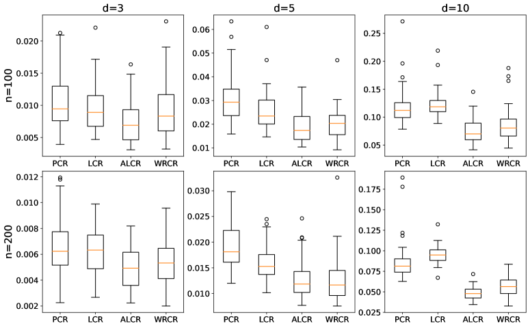
Figure 1: Table showing out-of-sample performance of four estimators for data Type I.

We next repeat this procedure with the Type B function, generating 50 replications of the MSE value for each of the LCR, PCR, ALCR, and WRCR estimators, and create box plots each with 50 MSE values. In Figure 1, each box plot shows the median (in the middle of each box), the first quantile (lower end of each box), the third quartile (higher end of each box), and outliers as small circles. Figure 1 shows the box plots for a wide range of $d$ when $n=100$ and $n=500$. Our proposed estimators, the ALCR and WRCR estimators, perform better than other estimators in most cases, especially when the dimension is higher, e.g., $d=10$.

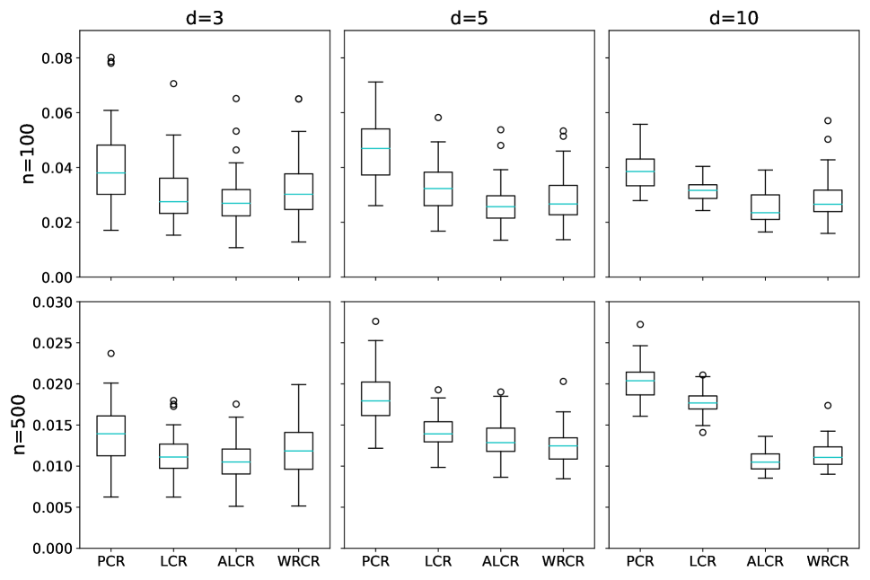
Figure 1: Each box plot is created with 50 MSE values for each of the PCR, LCR, ALCR, and WRCR estimators for difference values of $n$ and $d$. We use the Type B function.

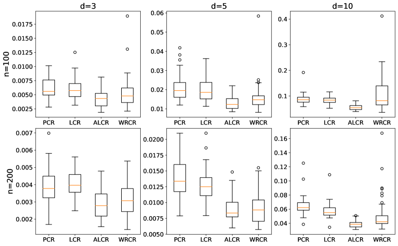
Figure 2: Table showing out-of-sample performance of four methods for data Type II.

We next use the Type B function to explore how the noise level affects the predictive performance of the proposed estimators. We repeat the previous experiment with the Type B function. Figure 2 reports the box plots each with 50 MSE values for a wide range of SNR$\in\{1.0,1.5,2.0,2.5,3.0\}$ when $n=100,d=3$ and when $n=500,d=10$.

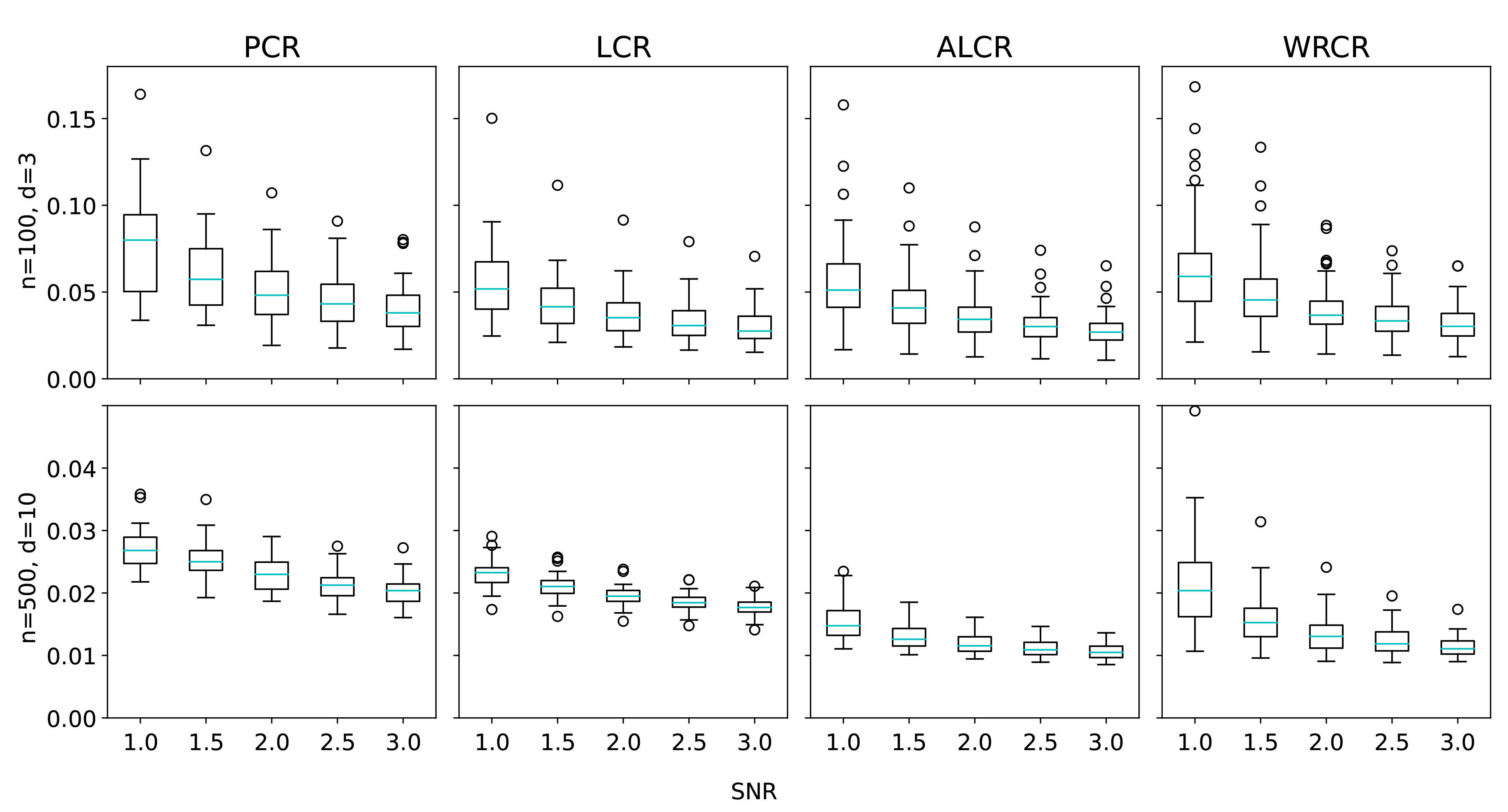
Figure 2: Each box plot is created with 50 MSE values for each of the PCR, LCR, ALCR, and WRCR estimators for different values of SNR. We use the Type B function.

LCR performs similarly to ALCR when the sample size is small ($n=100,d=3$). However, the new method shows better predictive power in large sample settings ($n=500,d=10$). In these settings, WRCR also performs reasonably well compared to other benchmarks but does not show such an advantage at high noise levels. The e-companion to this paper provides additional numerical results with different underlying functions $f_{0}$.

7 Regulation on Electricity Distribution Firms in Finland

In Finland, electricity distribution firms typically enjoy a natural local monopoly due to prohibitively expensive construction fees. This forces governments to establish regulatory agencies to monitor the electricity distribution firms, reduce their local monopoly power, and provide incentives to those adopting the best technology. The EV is one of the pioneers in practically implementing energy regulation programs, which involve cost-efficiency analysis for distribution firms. The traditional frontier estimation techniques, such as data envelopment analysis and stochastic frontier analysis, were applied by EV from 2005 to 2011, and a more reliable CR model was adopted from 2012 onward (Kuosmanen, 2012). Recently, EV considered developing new techniques to reduce the overfitting behaviour in CR and increase the accuracy of its incentive regulatory model for Finnish electricity distribution firms (Kuosmanen et al., 2022). In our analysis, we examine the performance of our proposed estimators on the cost frontier estimation problem for Finnish electricity distribution firms.

7.1 Frontier Estimation Model

We consider a general cost frontier model in production economics (Kuosmanen and Johnson, 2020):

$$y_{i}=C(\boldsymbol{x}_{i})+\varepsilon_{i}$$ (24)

for $i=1,\cdots,n$, where $C$ is a nondecreasing and convex cost function, and the $\varepsilon_{i}$’s are the error terms representing random effects. $\boldsymbol{x}_{i}$ is the vector of performance variables for firm $i$, and $y_{i}$ is the variable cost of firm $i$. The variables are specified as follows:

$$y =$$ Variable cost representing the controllable operational expenditure (KOPEX, €)

$$x(1) =$$ Energy supply (GWh, weighted by voltage)

$$x(2) =$$ Length of the network (km)

$$x(3) =$$ Number of user points

$$x(4) =$$ Fixed cost representing the capital stock (regulatory asset value, NKA, €)

We collect data from the EV over three regulation periods with 86 Finnish electricity distribution firms, covering the years from 2008 to 2020. The original dataset is applied to build the incentive regulation model for Finnish electricity distribution firms (Kuosmanen et al., 2022), and its earlier version has been widely used; see Kuosmanen (2012), Kuosmanen et al. (2013), and Kuosmanen and Johnson (2020) for details.

To estimate the cost function $C$ in (24), we consider the following variant of CR that incorporates the monotonicity of $C$:

$$\min_{\boldsymbol{\beta},\alpha,\varepsilon} \frac{1}{n}\sum_{i=1}^{n}\varepsilon_{i}^{2}$$ (25)

s.t. $$y_{i}=\alpha_{i}+\boldsymbol{\beta}_{i}^{T}\boldsymbol{x}_{i}+\varepsilon_{i} i=1,\cdots,n$$

$$\alpha_{i}+\boldsymbol{\beta}_{i}^{T}\boldsymbol{x}_{i}\geq\alpha_{j}+\boldsymbol{\beta}_{j}^{T}\boldsymbol{x}_{i} i,j=1,\cdots,n$$

$$\boldsymbol{\beta}_{i}\geq\boldsymbol{0} i=1,\cdots,n.$$

The last constraint in (25) guarantees that the estimated cost function is non-decreasing. The monotonicity assumption on production/cost function has been identified in various areas such as operations research and economics; see, for example, Kuosmanen and Johnson (2010) and Kuosmanen and Kortelainen (2012). However, the additional monotonicity constraint in (25) does not eliminate the overfitting behaviour.

Using our data set $((\boldsymbol{x}_{i},y_{i}):1\leq i\leq 1042)$, we compute the CR estimator and its subgradients $\hat{\boldsymbol{\beta}}_{i}=(\hat{\beta}_{i}(1),\hat{\beta}_{i}(2),\hat{\beta}_{i}(3),\hat{\beta}_{i}(4))$ at $\boldsymbol{x}_{i}$. Table 3 reports some summary statistics, such as the mean, standard deviation, minimum, 10th percentile, median, 90th percentile, and maximum, for $(\hat{\beta}_{i}(k):1\leq i\leq 1042)$ for each $k\in\{1,2,3,4\}$.

For each variable, the range between the minimum and maximum estimated subgradients is quite large. Those large subgradients usually occur near the boundary of the domain, and hence, lead to the overfitting behaviour in the CR estimator. The overfitting problem may lead to invalid results in frontier estimation and produce misleading benchmarks for the acceptable level of cost in future regulation periods.

The 90th percentiles indicate that the estimated subgradients within the 90th percentile should not be very large. We notice that the changes in the estimated subgradients are much smaller within the range between the 10th and 90th percentiles than in the range between the minimum and the maximum. This difference is caused by a few big firms with extreme data values that lead to overfitting behaviour in estimating the cost function using CR.

Table 3: Summary of the subgradients of the CR estimator with the Finnish electricity distribution firm data.

	$\hat{\beta}_{i}(1)$ (€ cents/kWh)	$\hat{\beta}_{i}(2)$ (€ /km)	$\hat{\beta}_{i}(3)$ (€ /customer)	$\hat{\beta}_{i}(4)$
Mean	2.7	0.6	66.8	27.1
Standard deviation	4.6	1.7	627.2	107.6
Minimum	0.0	0.0	0.0	0.0
10th percentile	0.0	0.0	0.1	0.1
Median	1.8	0.5	34.3	9.1
90th percentile	6.4	0.8	75.5	41.4
Maximum	69.4	39.5	19887.3	2385.4

The descriptive statistics in Table 3 provide some information that we can use in our proposed estimators. For example, the median values in Table 3 are natural candidates for $\boldsymbol{b}_{0}$ in the ALCR estimator.

7.2 Evaluating the Predictive Performance

For the next regulation period between 2024 and 2031, improving the predictive accuracy of the cost frontier model is one of the main concerns of EV regulators. In this section, we compare the two proposed estimators with several key benchmark methods that have been used on the Finnish electricity distribution firm data. For this purpose, we need to slightly modify the CR, PCR, ARCR, and WRCR estimators. The CR estimator (25) is a variant of the CR estimator where the monotonicity of the underlying function is incorporated as $\boldsymbol{\beta}_{i}\geq 0$ for $i=1,\cdots,n$ in the constraint. We also add these conditions to the constraints of PCR’s, LCR’s, ARCR’s, and WRCR’s formulations.

In all computations, we use the observations in the first 9 years $((\boldsymbol{a}_{i},b_{i}):i=1,\cdots,734)$ as the training data set and the observations in the last 4 years $((\boldsymbol{c}_{i},d_{i}):i=1,\cdots,308)$ as the test data set. We set $\boldsymbol{b}_{0}=(1.8,0.5,34.3,9.1)$ as the median values reported in Table 3. We use the training data set to compute all other tuning parameters, $\lambda$ in PCR, $L$ in LCR, $L_{0}$ in ARCR, and $q$ (defined in Remark 6) in WRCR. We use the 5-fold cross-validation method with the following set of candidate values: 50 equally spaced values from $[1,500]$ for each of $\lambda_{n}$, $L$ and $L_{0}$, and $\{0.01,0.02,\cdots,0.49\}$ for $q$. We next use the test data set to measure the accuracy of each estimator. For example, to measure the accuracy of the CR estimator, we define in-sample root mean square error (in-sample RMSE) as follows:

$$\left\{\frac{1}{734}\sum_{i=1}^{734}(b_{i}-\mbox{ CR at }\boldsymbol{a}_{i})^{2}\right\}^{1/2}$$

and out-of-sample root mean square error (out-of-sample RMSE) as follows:

$$\left\{\frac{1}{308}\sum_{i=1}^{308}(d_{i}-\mbox{CR at }\boldsymbol{c}_{i})^{2}\right\}^{1/2}.$$

Table 4 reports the in-sample and out-of-sample RMSEs for various estimators. The CR estimator results in a severe overfitting problem, where the in-sample RMSE is very small while the out-of-sample RMSE appears to be very large. The PCR, LCR, and our proposed estimators (ALCR and WRCR) yield results that are significantly better than those of CR, demonstrating that an additional bound on the subgradients helps improve the predictive performance of CR. We observe that the proposed estimators work best in terms of the prediction accuracy. The WRCR estimator achieves the smallest out-of-sample RMSEs, indicating that it outperforms other CR estimators in terms of predictive power.

Table 4: In-sample and out-of-sample RMSEs.

	CR	PCR	LCR	ALCR	WRCR
In-sample RMSE	1133.1	1384.4	1720.7	1619.1	1626.0
Out-of-sample RMSE	111255.4	1775.1	1748.4	1716.0	1644.9

From the regulator’s perspective, it can be hard to interpret the tuning parameter $\lambda_{n}$ in PCR and $L$ in LCR. This makes the model hard to be trusted by practitioners. By contrast, the tuning parameter $L_{0}$ in ALCR can be interpreted as the distance between the estimated marginal costs and the reference vector $\boldsymbol{b}_{0}$ (the median values of the subgradients of the CR estimator). The $q$th and $(1-q)$th percentiles used in the WRCR can be seen as the proportion of extreme values obtained from CR that the regulators would like to exclude from the subsequent estimation.

8 Conclusions

In this paper, we provide theoretical evidence of the overfitting behaviour of the CR and PCR estimators near the boundary of the domain. To eliminate the overfitting behaviour, we consider placing bounds on the subgradients of the fitted convex function. In particular, we propose two practical ways to set the bounds, leading our proposed estimators, the ALCR and WRCR estimators. Monte Carlo studies have shown the superior performance of our proposed estimators.

This work was initially motivated by the observed overfitting problem in the regulatory models previously used by the Finnish EV and the need to improve the prediction accuracy of their models in the 5th and 6th regulation periods from 2024 to 2031. The two newly proposed estimators allow EV to have a model that does not show the overfitting behaviour and outperforms the CR estimator.

There are several open research avenues. In this paper, we conducted numerical experiments in the cases where $d\ll n$. Understanding and investigating the behaviour of the CR estimator for larger dimensions is a direction of interest. Furthermore, the predictive performance of our approaches relies on the choice of tuning parameters. It would be interesting to develop a tuning-free CR model that does not show overfitting behaviour.

Disclosure statement

The authors report there are no competing interests to declare.

Appendix

A Proofs

To prove Theorem 1, we need Lemma 1 and Lemma 2, which are proved in Sections A.1 and A.2.

Lemma 1.

Consider the problem of minimizing

$$\sum_{i=1}^{n}(y_{i}+\alpha_{0}+\boldsymbol{\beta}_{0}^{T}\boldsymbol{x}_{i}-f(\boldsymbol{x}_{i}))^{2}$$ (A.1)

over $f\in\mathcal{F}$, for given $\alpha_{0}\in\mathbb{R}$ and $\boldsymbol{\beta}_{0}\in\mathbb{R}^{d}$. Then, $\hat{g}_{n}:\Omega\rightarrow\mathbb{R}$ defined by $\hat{g}_{n}(\boldsymbol{x})=\hat{f}_{n}(\boldsymbol{x})+\alpha_{0}+\boldsymbol{\beta}_{0}^{T}\boldsymbol{x}$ for $\boldsymbol{x}\in\Omega$ is a solution to (A.1).

Lemma 2.

Assume A1–A6. Suppose $\partial f_{0}(\boldsymbol{0})<\boldsymbol{0}$. Then, there exists $\epsilon_{0}>0$ such that for any $\epsilon<\epsilon_{0}$,

$$\liminf_{n\rightarrow\infty}\mathbb{P}(\hat{f}_{n}(\boldsymbol{0})>f_{0}(\boldsymbol{0})+\epsilon)>0.$$

A.1 Proof of Lemma 1

Proof.

Obviously, $\hat{g}_{n}$ belongs to $\mathcal{F}$. Now, we will show $\hat{g}_{n}$ is a minimizer of (A.1). For any $f\in\mathcal{F}$, $f(\boldsymbol{x})-\alpha_{0}-\boldsymbol{b}^{T}\boldsymbol{x}$ belongs to $\mathcal{F}$. Since $\hat{f}_{n}$ is a minimizer of (2), we have

$$\sum_{i=1}^{n}(y_{i}-\hat{f}_{n}(\boldsymbol{x}_{i})^{2}\leq\sum_{i=1}^{n}(y_{i}-(f(\boldsymbol{x}_{i})-\alpha_{0}-\boldsymbol{b}^{T}\boldsymbol{x}_{i}))^{2},$$

or equivalently,

$$\sum_{i=1}^{n}(y_{i}+\alpha_{0}+\boldsymbol{b}^{T}\boldsymbol{x}_{i}-(\hat{f}_{n}(\boldsymbol{x}_{i})+\alpha_{0}+\boldsymbol{b}^{T}\boldsymbol{x}_{i}))^{2}\leq\sum_{i=1}^{n}(y_{i}+\alpha_{0}+\boldsymbol{b}^{T}\boldsymbol{x}_{i}-f(\boldsymbol{x}_{i}))^{2}.$$

So,

$$\sum_{i=1}^{n}(y_{i}+\alpha_{0}+\boldsymbol{b}^{T}\boldsymbol{x}_{i}-\hat{g}_{n}(\boldsymbol{x}_{i}))^{2}\leq\sum_{i=1}^{n}(y_{i}+\alpha_{0}+\boldsymbol{b}^{T}\boldsymbol{x}_{i}-f(\boldsymbol{x}_{i}))^{2}$$

for any $f\in\mathcal{F}$, and hence, $\hat{g}_{n}$ minimizes (A.1). ∎

A.2 Proof of Lemma 2

Proof.

We choose $\boldsymbol{x}_{n,1}$ as follows. For any $c>0$, consider the following hyperplane in $[0,1]^{d}$:

$$H_{c}\triangleq\left\{(x(1),\cdots,x(d))\in[0,1]^{d}:x(1)+\cdots+x(d)\leq c\right\}.$$

We let $c_{0}$ be the smallest positive real value of $c$ such that $H_{c}$ intersects with $\{\boldsymbol{x}_{1},\cdots,\boldsymbol{x}_{n}\}$ at only one point. This is possible due to the fact that the $\boldsymbol{x}_{i}$’s have a continuous density function by A3(ii). Let $\boldsymbol{x}_{n,1}$ be the point that intersects with $H_{c_{0}}$; see Figure 3 for an illustration of $H_{c_{0}}$ and $\boldsymbol{x}_{n,1}$ when $d=2$ and $n=7$. Mathematically, $\boldsymbol{x}_{n,1}=\boldsymbol{x}_{k}$, where $k=\operatorname*{arg\,min}_{i\in\{1,\cdots,n\}}x_{i}(1)+\cdots+x_{i}(d)$. By A1, $\boldsymbol{x}_{n,1}$ exists uniquely almost surely.

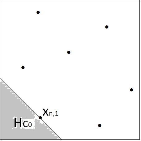
Figure 3: An illustration of $H_{c_{0}}$ and $\boldsymbol{x}_{n,1}$ when $d=2$ and $n=7$.

Since the $\boldsymbol{x}_{i}$’s are distinct a.s., there exists $\delta>0$ such that the rest of the $\boldsymbol{x}_{i}$’s belong to

$$\left\{(x(1),\cdots,x(d))\in[0,1]^{d}:x(1)+\cdots+x(d)>c+\delta\right\}.$$

It should be noted that there exists a convex function $h$ such that $h(\boldsymbol{x}_{n,1})=1$ and $h(\boldsymbol{x}_{j})=0$ for all $\boldsymbol{x}_{j}$’s satisfying $\boldsymbol{x}_{j}\neq\boldsymbol{x}_{n,1}$.

By (2.10) in Lemma 2.1 of Groeneboom (1996) (or Lemma 2.4 (i) and (ii) of Seijo and Sen, 2011), $\sum_{i=1}^{n}h(\boldsymbol{x}_{i})(\hat{f}_{n}(\boldsymbol{x}_{i})-y_{i})\geq 0$, or equivalently, $\hat{f}_{n}(\boldsymbol{x}_{n,1})-y_{n,1}\geq 0$, where $y_{n,1}$ is the observed value at $\boldsymbol{x}_{n,1}$. So,

$$\hat{f}_{n}(\boldsymbol{x}_{n,1})\geq y_{n,1}.$$ (A.2)

Note that since $f_{0}$ is convex and differentiable, it is continuously differentiable by Theorem 25.5 of Rockafellar (1997). Also, since $\nabla f_{0}(\boldsymbol{0})<\boldsymbol{0}$, there exists a neighborhood of $\boldsymbol{0}$, where $\nabla f_{0}(\boldsymbol{x})<\boldsymbol{0}$ for all $\boldsymbol{x}$ in that neighborhood. By A1, A2, A3(i), and A4–A6, $\nabla\hat{f}_{n}(\boldsymbol{x})$ converges to $\nabla f_{0}(\boldsymbol{x})$ a.s. as $n\rightarrow\infty$ uniformly over $[\delta,1-\delta]^{d}$ for any $\delta>0$ (See Theorem 3.1 (iv) of Seijo and Sen, 2011). By the convexity of $\hat{f}_{n}$, we can conclude that there exists a neighborhood of $\boldsymbol{0}$ such that $\boldsymbol{\beta}<\boldsymbol{0}$ for $\boldsymbol{\beta}\in\partial\hat{f}_{n}(\boldsymbol{x})<\boldsymbol{0}$ for all $\boldsymbol{x}$ in that neighborhood and for $n$ sufficiently large. Since $\boldsymbol{x}_{n,1}\rightarrow\boldsymbol{0}$ as $n\rightarrow\infty$ a.s., we can conclude

$$\hat{f}_{n}(\boldsymbol{0})>\hat{f}_{n}(\boldsymbol{x}_{n,1})$$ (A.3)

for $n$ sufficiently large a.s. By (A.2) and (A.3), $\hat{f}_{n}(\boldsymbol{0})>y_{n,1}$, and hence,

$$\hat{f}_{n}(\boldsymbol{0})-f_{0}(\boldsymbol{0}) > y_{n,1}-f_{0}(\boldsymbol{x}_{n,1})+f_{0}(\boldsymbol{x}_{n,1})-f_{0}(\boldsymbol{0})$$ (A.4)

$$\geq \varepsilon_{1}+o(1)$$

for $n$ sufficiently large a.s.

Since $\varepsilon_{1}$ is a mean zero non-degenerate random variable, we have

$$\mathbb{P}(\varepsilon_{1}>\epsilon_{0})>0$$ (A.5)

for some $\epsilon_{0}>0$.

By (A.4) and (A.5),

$$\liminf_{n\rightarrow\infty}\mathbb{P}(\hat{f}_{n}(\boldsymbol{0})>f_{0}(\boldsymbol{0})+\epsilon_{0})>0,$$

which completes the proof of Lemma 2. ∎

A.3 Proof of Theorem 1

Proof.

Suppose $\nabla f_{0}(\boldsymbol{0})<\boldsymbol{0}$. Then Theorem 1 is followed by Lemma 2. Suppose $\partial f_{0}(\boldsymbol{0})<\boldsymbol{0}$ does not hold. Then, there exists $\boldsymbol{b}\in\mathbb{R}^{d}$ such that $\nabla[f_{0}(\boldsymbol{x})-\boldsymbol{b}\boldsymbol{x}]|_{\boldsymbol{x}=\boldsymbol{0}}<\boldsymbol{0}$. Let $\hat{h}_{n}$ be the minimizer of

$$\sum_{i=1}^{n}(y_{i}-\boldsymbol{b}^{T}\boldsymbol{x}_{i}-f(\boldsymbol{x}_{i}))^{2}$$ (A.6)

over $f\in\mathcal{F}$. Then, by Lemma 1, $\hat{f}_{n}(\boldsymbol{x})-\boldsymbol{b}^{T}\boldsymbol{x}_{i}$ becomes a solution to (A.6). Since (A.6) can be written as $\sum_{i=1}^{n}(f_{0}(\boldsymbol{x})-\boldsymbol{b}^{T}\boldsymbol{x}_{i}+\varepsilon_{i}-f(\boldsymbol{x}_{i}))^{2}$ and $f_{0}(\boldsymbol{x})-\boldsymbol{b}^{T}\boldsymbol{x}$ has a subgradient at $\boldsymbol{0}$ which is less than $\boldsymbol{0}$, Lemma 2 implies there exists $\epsilon_{0}>0$ such that for any $\epsilon<\epsilon_{0}$,

$$\liminf_{n\rightarrow\infty}\mathbb{P}(\hat{f}_{n}(\boldsymbol{0})+\boldsymbol{b}^{T}\boldsymbol{0}>f_{0}(\boldsymbol{0})+\boldsymbol{b}^{T}\boldsymbol{0}+\epsilon)>0.$$

This proves Theorem 1 when $\partial f_{0}(\boldsymbol{0})<0$ doesn’t hold. ∎

A.4 Proof of Theorem 2

Proof.

We will prove that Theorem 2 follows from Theorem 1. Let $\epsilon_{0}$ be given as in Lemma 2. Let $M>0$ be given. Since $\hat{f}_{n}$ is convex, for any $\boldsymbol{x}\in[0,1]^{d}\backslash\{\boldsymbol{0}\}$ and any $\boldsymbol{\beta}\in\partial\hat{f}_{n}(\boldsymbol{0})$, we have $\hat{f}_{n}(\boldsymbol{\boldsymbol{0}})+\boldsymbol{\beta}^{T}\boldsymbol{x}\leq\hat{f}_{n}(\boldsymbol{x})$, and hence,

$$\hat{f}_{n}(\boldsymbol{0})\leq\hat{f}_{n}(\boldsymbol{x})+\|\boldsymbol{\beta}\|\|\boldsymbol{x}\|.$$

Since

$$\mathbb{P}(\hat{f}_{n}(\boldsymbol{0})>f_{0}(\boldsymbol{0})+\epsilon_{0})\leq\mathbb{P}(\hat{f}_{n}(\boldsymbol{x})>f_{0}(\boldsymbol{0})+\epsilon_{0}/2)+\mathbb{P}\left(\min_{\boldsymbol{\beta}\in\partial\hat{f}_{n}(\boldsymbol{0})}\|\boldsymbol{\beta}\|\|\boldsymbol{x}\|>\epsilon_{0}/2\right),$$

taking the liminf on both sides yields

$$\liminf_{n\rightarrow\infty}\mathbb{P}(\hat{f}_{n}(\boldsymbol{0})>f_{0}(\boldsymbol{0})+\epsilon_{0})$$ (A.7)

$$\leq \liminf_{n\rightarrow\infty}\left[\mathbb{P}(\hat{f}_{n}(\boldsymbol{x})>f_{0}(\boldsymbol{0})+\epsilon_{0}/2)+\mathbb{P}\left(\min_{\boldsymbol{\beta}\in\partial\hat{f}_{n}(\boldsymbol{0})}\|\boldsymbol{\beta}\|>\epsilon_{0}/(2\|\boldsymbol{x}\|)\right)\right].$$

Since $\hat{f}_{n}$ converges to $f_{0}$ uniformly on $[\delta,1-\delta]^{d}$ a.s. for any $\delta>0$ (Theorem 3.1 of Seijo and Sen, 2011) and $f_{0}$ is continuous (A6), we can take $\boldsymbol{x}$ close enough to $\boldsymbol{0}$ so that $\lim_{n\rightarrow\infty}\mathbb{P}(\hat{f}_{n}(\boldsymbol{x})>f_{0}(\boldsymbol{0})+\epsilon_{0}/2)=0$. From (A.7), it follows that

$$\liminf_{n\rightarrow\infty}\mathbb{P}(\hat{f}_{n}(\boldsymbol{0})>f_{0}(\boldsymbol{0})+\epsilon_{0})\leq\liminf_{n\rightarrow\infty}\mathbb{P}\left(\min_{\boldsymbol{\beta}\in\partial\hat{f}_{n}(\boldsymbol{0})}\|\boldsymbol{\beta}\|>\epsilon_{0}/(2\|\boldsymbol{x}\|)\right).$$ (A.8)

We can also take $\boldsymbol{x}$ close enough to $\boldsymbol{0}$ so that $\epsilon_{0}/(2\|\boldsymbol{x}\|)>M$. From (A.8) and Theorem 1, we obtain

$$\liminf_{n\rightarrow\infty}\mathbb{P}\left(\sup_{\boldsymbol{\beta}\in\partial\hat{f}_{n}(\boldsymbol{0})}\|\boldsymbol{\beta}\|>M\right)>\epsilon_{1},$$

for some real number $\epsilon_{1}>0$, which completes the proof of Theorem 2. ∎

A.5 Proof of Theorem 3

Suppose, on the contrary, that $\min_{\boldsymbol{\beta}\in\partial\hat{f}_{n,p}(\boldsymbol{x}_{n,1})}\|\boldsymbol{\beta}\|$ is bounded in probability. We will reach a contradiction.

Define $\phi:\mathbb{R}^{(d+1)n}\rightarrow\mathbb{R}$ by

$$\phi(g_{1},\cdots,g_{n},\boldsymbol{\beta}_{1},\cdots,\boldsymbol{\beta}_{n})=\frac{1}{n}\sum_{i=1}^{n}(y_{i}-g_{i})^{2}+\frac{\lambda_{n}}{n}\sum_{i=1}^{n}\|\boldsymbol{\beta}_{i}\|^{2}$$

for $g_{1},\cdots,g_{n}\in\mathbb{R}$ and $\boldsymbol{\beta}_{1},\cdots,\boldsymbol{\beta}_{n}\in\mathbb{R}^{d}$. Then $\phi$ is a continuous convex function. Let

$$\mathcal{K}=\{(g_{1},\cdots,g_{n},\boldsymbol{\beta}_{1},\cdots,\boldsymbol{\beta}_{n})\in\mathbb{R}^{(d+1)n}:g_{i}\geq g_{j}+\boldsymbol{\beta}_{j}^{T}(\boldsymbol{x}_{i}-\boldsymbol{x}_{j})\}.$$

Then, $\mathcal{K}$ is non-empty, convex cone and $\phi$ is differentiable.

Let $(\hat{g}_{1},\cdots,\hat{g}_{n},\hat{\boldsymbol{\beta}}_{1},\cdots,\hat{\boldsymbol{\beta}}_{n})$ minimise $\phi$ over $\mathcal{K}$. Then, by Lemma 2.1 and (2.11) of Groeneboom (1996), we have

$$-\frac{2}{n}\sum_{i=1}^{n}g_{i}(y_{i}-\hat{g}_{i})+\frac{2\lambda_{n}}{n}\sum_{i=1}^{n}\boldsymbol{\beta}_{i}\hat{\boldsymbol{\beta}}_{i}\geq 0$$ (A.9)

for any $(g_{1},\cdots,g_{n},\boldsymbol{\beta}_{1},\cdots,\boldsymbol{\beta}_{n})\in\mathcal{K}$. By the arguments similar to those in the proof of Lemma 2, there exists a convex function $h$ such that $h(\boldsymbol{x}_{n,1})=1$, $h(\boldsymbol{x}_{j})=0$ for all the $\boldsymbol{x}_{i}$’s satisfying $\boldsymbol{x}_{j}\neq\boldsymbol{x}_{n,1}$, and the gradient of $h$ at $\boldsymbol{x}_{n,1}$ is $(-1,-1,\cdots,-1)\in\mathbb{R}^{d}$. Applying (A.9) to this function yields

$$\hat{g}_{n,1}\geq y_{n,1}+\lambda_{n}\sum_{i=1}^{n}\hat{\boldsymbol{\beta}}_{i},$$ (A.10)

where $\hat{g}_{n,1}=\hat{f}_{n,p}(\boldsymbol{x}_{n,1})$ and $y_{n,1}$ is the value of the $y_{i}$’s at $\boldsymbol{x}_{n,1}$. From (A.10), it follows that

$$\hat{g}_{n,1}\geq y_{n,1}-\lambda_{n}\sum_{i=1}^{n}|\hat{\boldsymbol{\beta}}_{i}|.$$

Since $\min_{\boldsymbol{\beta}\in\partial\hat{f}_{n,p}(\boldsymbol{x}_{n,1})}\|\boldsymbol{\beta}\|$ is assumed to be bounded in probability and $\lambda_{n}\rightarrow 0$ as $n\rightarrow\infty$, we have

$$\hat{g}_{n,1}\geq y_{n,1}+o_{p}(1)$$

as $n\rightarrow\infty$. We can conclude

$$\liminf_{n\rightarrow\infty}\mathbb{P}(\hat{f}_{n,p}(\boldsymbol{x}_{n,1})\geq f_{0}(\boldsymbol{x}_{n,1})+\epsilon_{0})>0$$ (A.11)

for some $\epsilon_{0}>0$.

Let $M>0$ be given. Since $\hat{f}_{n,p}$ is convex, for any $\boldsymbol{x}\in[0,1]^{d}\backslash\{\boldsymbol{x}_{n,1}\}$ and any $\boldsymbol{\beta}\in\partial\hat{f}_{n}(\boldsymbol{x}_{n,1})$, we have $\hat{f}_{n,p}(\boldsymbol{x}_{n,1})+\boldsymbol{\beta}^{T}(\boldsymbol{x}-\boldsymbol{x}_{n,1})\leq\hat{f}_{n,p}(\boldsymbol{x})$, and hence,

$$\hat{f}_{n,p}(\boldsymbol{x}_{n,1})\leq\hat{f}_{n,p}(\boldsymbol{x})+\min_{\boldsymbol{\beta}\in\partial\hat{f}_{n}(\boldsymbol{x}_{n,1})}\|\boldsymbol{\beta}\|\|\boldsymbol{x}-\boldsymbol{x}_{n,p}\|.$$

Since

$$\mathbb{P}(\hat{f}_{n,p}(\boldsymbol{x}_{n,1})>f_{0}(\boldsymbol{x}_{n,1})+\epsilon_{0})\\ \leq\mathbb{P}(\hat{f}_{n,p}(\boldsymbol{x}_{n,1})>f_{0}(\boldsymbol{x}_{n,1})+\epsilon_{0}/2)+\mathbb{P}\left(\min_{\boldsymbol{\beta}\in\partial\hat{f}_{n}(\boldsymbol{x}_{n,1})}\|\boldsymbol{\beta}\|\|\boldsymbol{x}-\boldsymbol{x}_{n,1}\|>\epsilon_{0}/2\right),$$

taking the liminf on both sides yields

$$\liminf_{n\rightarrow\infty}\mathbb{P}(\hat{f}_{n,p}(\boldsymbol{x}_{n,1})>f_{0}(\boldsymbol{x}_{n,1})+\epsilon_{0})\\ \leq\liminf_{n\rightarrow\infty}\Bigg{[}\mathbb{P}(\hat{f}_{n,p}(\boldsymbol{x})>f_{0}(\boldsymbol{x}_{n,1})+\epsilon_{0}/2)\\ +\mathbb{P}\left(\min_{\boldsymbol{\beta}\in\partial\hat{f}_{n}(\boldsymbol{x}_{n,1})}\|\boldsymbol{\beta}\|>\epsilon_{0}/(2\|\boldsymbol{x}-\boldsymbol{x}_{n,1}\|)\right)\Bigg{]}.$$ (A.12)

Since $\hat{f}_{n,p}$ converges to $f_{0}$ uniformly on $[\delta,1-\delta]^{d}$ a.s. for any $\delta>0$ (Theorem 1 of Lim, 2021) and $f_{0}$ is continuous (A6), we can take $\boldsymbol{x}$ close enough to $\boldsymbol{0}$ so that $\lim_{n\rightarrow\infty}\mathbb{P}(\hat{f}_{n,p}(\boldsymbol{x})>f_{0}(\boldsymbol{x}_{n,1})+\epsilon_{0}/2)=0$. From (A.12), it follows that

$$\liminf_{n\rightarrow\infty}\mathbb{P}(\hat{f}_{n,p}(\boldsymbol{x}_{n,1})>f_{0}(\boldsymbol{x}_{n,1})+\epsilon_{0})\leq\liminf_{n\rightarrow\infty}\mathbb{P}\left(\min_{\boldsymbol{\beta}\in\partial\hat{f}_{n}(\boldsymbol{0})}\|\boldsymbol{\beta}\|>\epsilon_{0}/(2\|\boldsymbol{x}-\boldsymbol{x}_{n,1}\|)\right).$$ (A.13)

We can also take $\boldsymbol{x}$ close enough to $\boldsymbol{0}$ so that $\epsilon_{0}/(2\|\boldsymbol{x}\|)>M$. From (A.11) and (A.13), we obtain

$$\liminf_{n\rightarrow\infty}\mathbb{P}\left(\sup_{\boldsymbol{\beta}\in\partial\hat{f}_{n}(\boldsymbol{x}_{n,1})}\|\boldsymbol{\beta}\|>M\right)>\epsilon_{2}$$

for some real number $\epsilon_{2}>0$, which is a contradiction.

A.6 Proof of Theorem 4

We first prove (i), and then show that (i) implies (ii).

Proof.

The proof of (i) consists of 13 steps.

Step 1: We use A5, A7, and the fact that $\hat{f}_{n,A}$ is a minimizer of $\sum_{i=1}^{n}(y_{i}-f(\boldsymbol{x}_{i}))^{2}$ over $f\in\mathcal{F}_{A}$ to obtain

$$\frac{1}{n}\sum_{i=1}^{n}(\hat{f}_{n,A}(\boldsymbol{x}_{i})-f_{0}(\boldsymbol{x}_{i}))^{2}\leq\frac{2}{n}\sum_{i=1}^{n}\varepsilon_{i}(\hat{f}_{n,A}(\boldsymbol{x}_{i})-f_{0}(\boldsymbol{x}_{i})).$$ (A.14)

To prove (A.14), note that $f_{0}\in\mathcal{F}_{A}$ by A5 and A7 and that $\hat{f}_{n,A}$ is a minimizer of (14). So, we have

$$\frac{1}{n}\sum_{i=1}^{n}(y_{i}-f_{n,A}(\boldsymbol{x}_{i}))^{2}\leq\frac{1}{n}\sum_{i=1}^{n}(y_{i}-f_{0}(\boldsymbol{x}_{i}))^{2},$$

or equivalently,

$$\frac{1}{n}\sum_{i=1}^{n}(f_{0}(\boldsymbol{x}_{i})+\varepsilon_{i}-f_{n,A}(\boldsymbol{x}_{i}))^{2}\leq\frac{1}{n}\sum_{i=1}^{n}(f_{0}(\boldsymbol{x}_{i})+\varepsilon_{i}-f_{0}(\boldsymbol{x}_{i}))^{2},$$

which leads to (A.14).

Step 2: We use A1, A2, A4, and (A.14) to prove that there exists a constant $c_{0}$ such that

$$\frac{1}{n}\sum_{i=1}^{n}\hat{f}_{n,A}(\boldsymbol{x}_{i})^{2}\leq c_{0}$$ (A.15)

for $n$ sufficiently large a.s.

To prove (A.15), note that

$$\frac{1}{n}\sum_{i=1}^{n}f_{n,A}(\boldsymbol{x}_{i})^{2} \leq \frac{1}{n}\sum_{i=1}^{n}(f_{n,A}(\boldsymbol{x}_{i})-f_{0}(\boldsymbol{x}_{i})+f_{0}(\boldsymbol{x}_{i}))^{2}$$ (A.16)

$$\leq \frac{2}{n}\sum_{i=1}^{n}(f_{n,A}(\boldsymbol{x}_{i})-f_{0}(\boldsymbol{x}_{i}))^{2}+\frac{2}{n}\sum_{i=1}^{n}f_{0}(\boldsymbol{x}_{i})^{2}.$$

On the other hand, applying the Cauchy-Schwarz inequality to the right-hand side of (A.14) yields

$$\frac{1}{n}\sum_{i=1}^{n}(\hat{f}_{n,A}(\boldsymbol{x}_{i})-f_{0}(\boldsymbol{x}_{i}))^{2}\leq 2\sqrt{\frac{1}{n}\sum_{i=1}^{n}\varepsilon_{i}^{2}}\sqrt{\frac{1}{n}\sum_{i=1}^{n}(f_{n,A}(\boldsymbol{x}_{i})-f_{0}(\boldsymbol{x}_{i}))^{2}},$$

so we have

$$\frac{1}{n}\sum_{i=1}^{n}(f_{n,A}(\boldsymbol{x}_{i})-f_{0}(\boldsymbol{x}_{i}))^{2}\leq\frac{4}{n}\sum_{i=1}^{n}\varepsilon_{i}^{2}.$$ (A.17)

Combining (A.16) and (A.17) yields

$$\frac{1}{n}\sum_{i=1}^{n}f_{n,A}(\boldsymbol{x}_{i})^{2}\leq\frac{8}{n}\sum_{i=1}^{n}\varepsilon_{i}^{2}+\frac{2}{n}\sum_{i=1}^{n}f_{0}(\boldsymbol{x}_{i})^{2}.$$

By A1, A2, A4, and the strong law of large numbers,

$$\frac{1}{n}\sum_{i=1}^{n}f_{n,A}(\boldsymbol{x}_{i})^{2}\leq 8\boldsymbol{E}[\varepsilon_{1}^{2}]+2\boldsymbol{E}[f_{0}(\boldsymbol{x}_{1})^{2}]+1\triangleq c_{0}$$

for $n$ sufficiently large a.s.

Step 3: In the following steps, we will use the following lemma, which is Lemma 1 of Luo and Lim (2016).

Let $\boldsymbol{e}_{0}=(0,0,\cdots,0)^{T}$. For $1\leq i\leq d$, let $\boldsymbol{e}_{i}\in\mathbb{R}^{d}$ be the vector of zeros except 1 in the $i$th entry. Let $\boldsymbol{v}_{*}=(1/(4d),1/d,\cdots,$ $1/d)$. Let $A_{i}$ be defined as follows:

$$A_{0} = \left\{x\in[0,1]^{d}:\|\boldsymbol{x}-\boldsymbol{e}_{0}\|\leq\tau\right\},$$

$$A_{1} = [1/2,1]\times[0,1]\times\dots\times[0,1]\subset[0,1]^{d},$$

$$A_{i} = \left\{x\in[0,1]^{d}:\|\boldsymbol{x}-\boldsymbol{e}_{i}\|\leq\tau\right\}\mbox{ for }2\leq i\leq d,$$

$$A_{d+1} = \left\{x\in[0,1]^{d}:\|\boldsymbol{x}-\boldsymbol{v}_{*}\|\leq\tau\right\}.$$

Then there exists a positive constant $\tau_{*}$ such that $0\leq\tau\leq\tau_{*}$ implies for any $\boldsymbol{y}$ in $A_{d+1}$ and $\boldsymbol{z}_{i}$ in $A_{i}$ for $0\leq i\leq d$, there exist nonnegative real numbers $p_{0},p_{1},\dots,p_{d}$ summing to one such that

$$p_{0}\boldsymbol{z}_{0}+p_{1}\boldsymbol{z}_{1}+\dots+p_{d}\boldsymbol{z}_{d}=\boldsymbol{y}$$

and that $p_{1}\geq 1/(16d)$.

Step 4: In the following steps, we will also use the following lemma, which is Lemma 2 of Luo and Lim (2016).

For $0\leq i\leq d$, let $\boldsymbol{u}_{i}$ be the vector identical to $\boldsymbol{e}_{i}$ except that its first element is one minus $\boldsymbol{e}_{i}$’s first element. Let $\boldsymbol{w}_{*}=(1-1/(4d),1/d,\cdots,1/d)$. Let $B_{i}$ be defined as follows:

$$B_{0} = \left\{\boldsymbol{x}\in[0,1]^{d}:\|\boldsymbol{x}-\boldsymbol{u}_{0}\|\leq\tau\right\},$$

$$B_{1} = [0,1/2]\times[0,1]\times\dots\times[0,1]\subset[0,1]^{d},$$

$$B_{i} = \left\{\boldsymbol{x}\in[0,1]^{d}:\|\boldsymbol{x}-\boldsymbol{u}_{i}\|\leq\tau\right\}\mbox{ for }2\leq i\leq d,$$

$$B_{d+1} = \left\{\boldsymbol{x}\in[0,1]^{d}:\|\boldsymbol{x}-\boldsymbol{w}_{*}\|\leq\tau\right\}.$$

Then, there exists a positive constant $\tau_{*}$ such that $0\leq\tau\leq\tau_{*}$ implies for any $\boldsymbol{y}$ in $B_{d+1}$ and $\boldsymbol{z}_{i}$ in $B_{i}$ for $0\leq i\leq d$, there exist nonnegative real numbers $p_{0},p_{1},\dots,p_{d}$ summing to one such that

$$p_{0}\boldsymbol{z}_{0}+p_{1}\boldsymbol{z}_{1}+\dots+p_{d}\boldsymbol{z}_{d}=\boldsymbol{y}$$

and that $p_{1}\geq 1/(16d)$.

Step 5: We use Step 2, Step 3, Step 4, and A3(i) to establish that there exists a constant $r_{0}$ such that

$$\inf_{\boldsymbol{x}_{i}\in A_{j}}|\hat{f}_{n,A}(\boldsymbol{x}_{i})|\leq r_{0}$$ (A.18)

and

$$\inf_{\boldsymbol{x}_{i}\in B_{j}}|\hat{f}_{n,A}(\boldsymbol{x}_{i})|\leq r_{0}$$ (A.19)

for all $j=0,1,\cdots,d+1$ and for $n$ sufficiently large a.s.

To fill in the details, we note that, for any $j\in\{0,1,\cdots,d+1\}$ and $r>0$,

$$\frac{1}{n}\sum_{i=1}^{n}I(\boldsymbol{x}_{i}\in A_{j},|\hat{f}_{n,A}(\boldsymbol{x}_{i})|\leq r)\geq\frac{1}{n}\sum_{i=1}^{n}I(\boldsymbol{x}_{i}\in A_{j})-\frac{1}{n}\sum_{i=1}^{n}I(\boldsymbol{x}_{i}\in A_{j},|\hat{f}_{n,A}(\boldsymbol{x}_{i})|>r).$$ (A.20)

By Step 2 and Markov inequality,

$$\frac{1}{n}\sum_{i=1}^{n}I(\boldsymbol{x}_{i}\in A_{j},|\hat{f}_{n,A}(\boldsymbol{x}_{i})|>r)\leq\frac{1}{r^{2}}\cdot\frac{1}{n}\sum_{i=1}^{n}\hat{f}_{n,A}(\boldsymbol{x}_{i})^{2}$$

for $n$ sufficiently large. Choose $r_{0}$ so large that $(c_{0}+1)/r_{0}^{2}\leq 1/2\min_{0\leq j\leq d+1}\mathbb{P}(\boldsymbol{x}_{1}\in A_{j})$, then

$$\frac{1}{n}\sum_{i=1}^{n}I(\boldsymbol{x}_{i}\in A_{j},|\hat{f}_{n,A}(\boldsymbol{x}_{i})|\leq r_{0})>\frac{1}{2}\min_{0\leq j\leq d+1}\mathbb{P}(\boldsymbol{x}_{1}\in A_{j})$$

for $n$ sufficiently large a.s. By A3(i), $\min_{0\leq j\leq d+1}\mathbb{P}(\boldsymbol{x}_{1}\in A_{j})>0$. By the strong law of large numbers,

$$\frac{1}{n}\sum_{i=1}^{n}I(\boldsymbol{x}_{i}\in A_{j})\rightarrow\mathbb{P}(\boldsymbol{x}_{1}\in A_{j})$$

as $n\rightarrow\infty$ a.s. and

$$\liminf_{n\rightarrow\infty}\frac{1}{n}\sum_{i=1}^{n}I(\boldsymbol{x}_{i}\in A_{j},|\hat{f}_{n,A}(\boldsymbol{x}_{i})|\leq r)>0.$$

So, for $n$ sufficiently large, there exist $\boldsymbol{x}_{I(j)}\in A_{j}$ with $1\leq I(j)\leq n$ such that $|\hat{f}_{n,A}(\boldsymbol{x}_{I(j)})|\leq r_{0}$. So, (A.18) is established. (A.19) follows in a similar way.

Step 6: We use Step 3, Step 5, and the convexity of $\hat{f}_{n,A}$ to establish that

$$\inf_{\boldsymbol{x}\in[0,1]^{d}}\hat{f}_{n,A}(\boldsymbol{x})\geq-64r_{0}d$$

for $n$ sufficiently large a.s.

We will first establish $\inf_{\boldsymbol{x}\in A_{1}}\hat{f}_{n,A}(\boldsymbol{x})\geq-64r_{0}d$ for $n$ sufficiently large a.s., and then show $\inf_{\boldsymbol{x}\in B_{1}}\hat{f}_{n,A}(\boldsymbol{x})\geq-64r_{0}d$ for $n$ sufficiently large a.s.

To fill in the details, suppose that there exists $\boldsymbol{z}_{1}\in A_{1}$ and

$$\hat{f}_{n,A}(\boldsymbol{z}_{1})<-64r_{0}d$$

for some $n$ sufficiently large.

By Step 3 and Step 5, for any $\boldsymbol{y}\in A_{d+1}$, there exist $\boldsymbol{z}_{0}\in A_{0},\boldsymbol{z}_{2}\in A_{2},\cdots,\boldsymbol{z}_{d}\in A_{d}$ and nonnegative real numbers $p_{0},p_{1},\cdots,p_{d}$ satisfying

$$|\hat{f}_{n,A}(\boldsymbol{z}_{i})|\leq r_{0}\mbox{ for }i=0,2,\cdots,d,$$ (A.21)

$$p_{0}\boldsymbol{z}_{0}+p_{1}\boldsymbol{z}_{1}+p_{2}\boldsymbol{z}_{2}+\cdots+p_{d}\boldsymbol{z}_{d}=\boldsymbol{y},$$

$$p_{0}+p_{1}+\cdots+p_{d}=1,\mbox{ and}$$

$$p_{1}>1/(16d).$$

By the convexity of $\hat{f}_{n,A}$, we have

$$\hat{f}_{n,A}(\boldsymbol{y}) \leq \hat{f}_{n,A}(p_{0}\boldsymbol{z}_{0}+p_{1}\boldsymbol{z}_{1}+\cdots+p_{d}\boldsymbol{z}_{d})$$

$$\leq p_{0}\hat{f}_{n,A}(\boldsymbol{z}_{0})+p_{1}\hat{f}_{n,A}(\boldsymbol{z}_{1})+p_{2}\hat{f}_{n,A}(\boldsymbol{z}_{2})+\cdots+p_{d}\hat{f}_{n,A}(\boldsymbol{z}_{d}).$$

Since $\hat{f}_{n,A}(\boldsymbol{z}_{1})\leq-64r_{0}d$, $p_{1}>1/(16d)$, and (A.21) imply

$$\hat{f}_{n,A}(\boldsymbol{y})\leq-3r_{0},$$

and hence,

$$\inf_{\boldsymbol{x}\in A_{d+1}}|\hat{f}_{n,A}(\boldsymbol{x})|>r_{0},$$

which contradicts Step 5. So, we have $\inf_{\boldsymbol{x}\in A_{1}}\hat{f}_{n,A}(\boldsymbol{x})\geq-64r_{0}d$ for all $n$ sufficiently large. Similarly, we have $\inf_{\boldsymbol{x}\in B_{1}}\hat{f}_{n,A}(\boldsymbol{x})\geq-64r_{0}d$.

Step 7: We use the convexity of $\hat{f}_{n,A}$ and Step 2 to show that for any $\delta>0$, there exists a constant $c_{\delta}$ satisfying

$$\sup_{\boldsymbol{x}\in[\delta,1-\delta]^{d}}\hat{f}_{n,A}(\boldsymbol{x})\leq c_{\delta}$$

for $n$ sufficiently large a.s. For a complete proof, see the proof of Lemma 4 of Luo and Lim (2016).

Step 8: There exists a constant $c_{1}$ such that

$$|\hat{f}_{n,A}(\boldsymbol{x})-\hat{f}_{n,A}(\boldsymbol{y})|\leq c_{1}\|\boldsymbol{x}-\boldsymbol{y}\|$$ (A.22)

for any $\boldsymbol{x},\boldsymbol{y}\in[0,1]^{d}$ and $n=1,2,\cdots$ a.s.

(A.22) follows from the fact that $\hat{f}_{n,A}$ is a convex function having its subgradients bounded uniformly over $[0,1]^{d}$ and $n$, so $\hat{f}_{n,A}$ is Lipshitz with a Lipshitz constant uniformly on $n$ and over $[0,1]^{d}$.

Step 9: We use Step 6, Step 7, and Step 8 to establish there exists a constant $\gamma$ such that

$$\sup_{\boldsymbol{x}\in[0,1]^{d}}|\hat{f}_{n,A}(\boldsymbol{x})|\leq\gamma$$ (A.23)

for $n$ sufficiently large a.s.

To show (A.23), we note that by Step 6 and Step 7, there is a constant $c$ satisfying

$$\sup_{\boldsymbol{x}\in[0.1,0.9]^{d}}|\hat{f}_{n,A}(\boldsymbol{x})|<c$$ (A.24)

for $n$ sufficiently large a.s. Let $\boldsymbol{x}_{0}$ be any arbitrary point in $[0.1,0.9]^{d}$. For any $\boldsymbol{y}\in[0,1]^{d}\backslash[0.1,0.9]^{d}$, Step 8 and (A.24) imply

$$|\hat{f}_{n,A}(\boldsymbol{y})|\leq|\hat{f}_{n,A}(\boldsymbol{x})|+c_{1}\|\boldsymbol{x}-\boldsymbol{y}\|\leq c+c_{1}d\triangleq\gamma$$

for $n$ sufficiently large a.s., which proves Step 9.

Step 10: We note that for any $\epsilon>0$, there is a finite number of functions $f_{1},\cdots,f_{r}$ in

$$\tilde{\mathcal{F}}_{A}\triangleq\{f:[0,1]^{d}\rightarrow\mathbb{R}:f\mbox{ is convex, }|f(\boldsymbol{x})-f(\boldsymbol{y})|\leq c_{1}\|\boldsymbol{x}-\boldsymbol{y}\|\mbox{ for }\boldsymbol{x},\boldsymbol{y}\in[0,1]^{d},\sup_{\boldsymbol{x}\in[0,1]^{d}}|f(\boldsymbol{x})|\leq\gamma\}$$

with $r=r(\epsilon)$ satisfying, for any $f\in\tilde{\mathcal{F}}_{A}$,

$$\sup_{\boldsymbol{x}\in[0,1]^{d}}|f(\boldsymbol{x})-f_{i}(\boldsymbol{x})|<\epsilon$$ (A.25)

for some $i\in\{1,\cdots,r\}$. (A.25) follows from Step 8, Step 9, and Theorem 6 of Bronshtein (1976).

Step 11: We now use Step 10 and the strong law of large numbers to show that

$$\limsup_{n\rightarrow\infty}\frac{1}{n}\sum_{i=1}^{n}\varepsilon_{i}(\hat{f}_{n,A}(\boldsymbol{x}_{i})-f_{0}(\boldsymbol{x}_{i}))\leq 0$$ (A.26)

a.s. To fill in the details, let $\epsilon>0$ be given and select $f_{1},\cdots,f_{r}$ as suggested in Step 10. Then, for each $j\in\{1,\cdots,r\}$, we have

$$\frac{1}{n}\sum_{i=1}^{n}\varepsilon_{i}(\hat{f}_{n,A}(\boldsymbol{x}_{i})-f_{0}(\boldsymbol{x}_{i}))$$

$$\leq \frac{1}{n}\sum_{i=1}^{n}\varepsilon_{i}(\hat{f}_{n,A}(\boldsymbol{x}_{i})-f_{j}(\boldsymbol{x}_{i}))+\frac{1}{n}\sum_{i=1}^{n}\varepsilon_{i}(f_{j}(\boldsymbol{x}_{i})-f_{0}(\boldsymbol{x}_{i}))$$

$$\leq \frac{1}{n}\sum_{i=1}^{n}|\varepsilon_{i}|\sup_{\boldsymbol{x}\in[0,1]^{d}}|\hat{f}_{n,A}(\boldsymbol{x})-f_{j}(\boldsymbol{x})|+\max_{1\leq j\leq r}\frac{1}{n}\sum_{i=1}^{n}\varepsilon_{i}(f_{j}(\boldsymbol{x}_{i})-f_{0}(\boldsymbol{x}_{i}))$$

So,

$$\frac{1}{n}\sum_{i=1}^{n}\varepsilon_{i}(\hat{f}_{n,A}(\boldsymbol{x}_{i})-f_{0}(\boldsymbol{x}_{i}))$$

$$\leq \left[\min_{1\leq j\leq r}\sup_{\boldsymbol{x}\in[0,1]^{d}}|\hat{f}_{n,A}(\boldsymbol{x})-f_{j}(\boldsymbol{x})|\right]\left[\frac{1}{n}\sum_{i=1}^{n}|\varepsilon_{i}|\right]+\max_{1\leq j\leq r}\frac{1}{n}\sum_{i=1}^{n}\varepsilon_{i}(f_{j}(\boldsymbol{x}_{i})-f_{0}(\boldsymbol{x}_{i}))$$

$$\leq \frac{\epsilon}{n}\sum_{i=1}^{n}|\varepsilon_{i}|+\max_{1\leq j\leq r}\frac{1}{n}\sum_{i=1}^{n}\varepsilon_{i}(f_{j}(\boldsymbol{x}_{i})-f_{0}(\boldsymbol{x}_{i}))$$

$$\leq \epsilon(\mathbb{E}[|\varepsilon_{1}|]+1)+\epsilon$$

for $n$ sufficiently large a.s. by A1 and A2, and hence, (A.26) follows.

Step 12: By combining Step 1 and Step 11, we obtain

$$\frac{1}{n}\sum_{i=1}^{n}(\hat{f}_{n,A}(\boldsymbol{x}_{i})-f_{0}(\boldsymbol{x}_{i}))^{2}\rightarrow 0$$

as $n\rightarrow\infty$ a.s.

Step 13: We use Step 12 and the fact that $\hat{f}_{n,A}$ and $f_{0}$ are Lipschitz over $[0,1]^{d}$ to complete the proof of (i).

Let $\epsilon>0$ be given. Since $\Omega=[0,1]^{d}$ is compact, there exists a finite collection of sets $S_{1},\cdots,S_{l}$ covering $\Omega$, each having a diameter less than $\epsilon$, i.e., $\|\boldsymbol{x}-\boldsymbol{y}\|\leq\epsilon$ for any $\boldsymbol{x},\boldsymbol{y}\in S_{j}$ and $1\leq j\leq l$. By A7 and Step 4, there exists a Lipschitz constant, say $\lambda$, for both $\hat{f}_{n,A}$ and $f_{0}$ over $[0,1]^{d}$. For each $\boldsymbol{x}\in S_{j}$ and $\boldsymbol{x}_{i}\in S_{j}$,

$$|\hat{f}_{n,A}(\boldsymbol{x})-f_{0}(\boldsymbol{x})|$$

$$\leq |\hat{f}_{n,A}(\boldsymbol{x})-\hat{f}_{n,A}(\boldsymbol{x}_{i})|+|\hat{f}_{n,A}(\boldsymbol{x}_{i})-f_{0}(\boldsymbol{x}_{i})|+|f_{0}(\boldsymbol{x}_{i})-f_{0}(\boldsymbol{x})|$$

$$\leq 2\epsilon\lambda+|\hat{f}_{n,A}(\boldsymbol{x}_{i})-f_{0}(\boldsymbol{x}_{i})|.$$

So, for any $\boldsymbol{x}\in S_{j}$,

$$|\hat{f}_{n,A}(\boldsymbol{x})-f_{0}(\boldsymbol{x})|\leq 2\epsilon\lambda+\min_{\boldsymbol{x}_{i}\in S_{j}}|\hat{f}_{n,A}(\boldsymbol{x}_{i})-f_{0}(\boldsymbol{x}_{i})|.$$

Therefore,

$$\sup_{\boldsymbol{x}\in S_{j}}|\hat{f}_{n,A}(\boldsymbol{x})-f_{0}(\boldsymbol{x})|$$

$$\leq 2\epsilon\lambda+\min_{\boldsymbol{x}_{i}\in S_{j}}|\hat{f}_{n,A}(\boldsymbol{x}_{i})-f_{0}(\boldsymbol{x}_{i})|$$

$$\leq 2\epsilon\lambda+\left(\frac{1}{n}\sum_{i=1}^{n}|\hat{f}_{n,A}(\boldsymbol{x}_{i})-f_{0}(\boldsymbol{x}_{i})|I(\boldsymbol{x}_{i}\in S_{j})\right)\left(\frac{n}{\sum_{i=1}^{n}I(\boldsymbol{x}_{i}\in S_{j})}\right)$$

$$\leq 2\epsilon\lambda+\sqrt{\frac{1}{n}\sum_{i=1}^{n}(\hat{f}_{n,A}(\boldsymbol{x}_{i})-f_{0}(\boldsymbol{x}_{i}))^{2}}\left(\frac{n}{\sum_{i=1}^{n}I(\boldsymbol{x}_{i}\in S_{j})}\right).$$

By Step 12, A1 and A3(i), we conclude

$$\limsup_{n\rightarrow\infty}\sup_{\boldsymbol{x}\in S_{j}}|\hat{f}_{n,A}(\boldsymbol{x})-f_{0}(\boldsymbol{x})|\leq 2\epsilon\lambda$$

a.s. Since $\epsilon$ is arbitrary and there are finitely many $S_{j}$’s, we conclude

$$\sup_{\boldsymbol{x}\in[0,1]^{d}}|\hat{f}_{n,A}(\boldsymbol{x})-f_{0}(\boldsymbol{x})|\rightarrow 0$$

a.s. as $n\rightarrow\infty$, completing the proof of (i).

Next, we show that (i) implies (ii).

Suppose, on the contrary, that there exists $\epsilon_{0}>0$ and $\boldsymbol{z}_{1},\boldsymbol{z}_{2},\cdots\in[0,1]^{d}$ such that

$$\|\boldsymbol{\beta}-\nabla f_{0}(\boldsymbol{z}_{n})\|\geq\epsilon_{0}$$

for some $\boldsymbol{\beta}\in\partial\hat{f}_{n,A}(\boldsymbol{z}_{n})$ and infinitely many $n$ with a positive probability. It follows that there is $i\in\{1,\cdots,d\}$ satisfying

$$|\boldsymbol{e}_{i}^{T}\boldsymbol{\beta}-\boldsymbol{e}_{i}^{T}\nabla f_{0}(\boldsymbol{z}_{n})|\geq\epsilon_{0}/d$$ (A.27)

for some $\beta\in\partial\hat{f}_{n,A}(\boldsymbol{z}_{n})$ and infinitely many $n$ with positive probability, where $\boldsymbol{e}_{i}\in\mathbb{R}^{d}$ is the vector of zeros except for 1 in the $i$th entry for $1\leq i\leq d$.

(A.27) implies either

$$\boldsymbol{e}_{i}^{T}\boldsymbol{\beta}\geq\boldsymbol{e}_{i}^{T}\nabla f_{0}(\boldsymbol{z}_{n})+\epsilon_{0}/d$$ (A.28)

or

$$\boldsymbol{e}_{i}^{T}\nabla f_{0}(\boldsymbol{z}_{n})-\epsilon_{0}/d\geq\boldsymbol{e}_{i}^{T}\boldsymbol{\beta}$$ (A.29)

for some $\boldsymbol{\beta}\in\partial\hat{f}_{n,A}(\boldsymbol{z}_{n})$ and infinitely many $n$ with positive probability. We will consider the case where (A.28) holds and reaches a contradiction. Similar arguments can be applied when (A.29) holds.

When (A.28) holds, there exists a subsequence $\boldsymbol{z}_{n_{1}},\boldsymbol{z}_{n_{2}},\cdots$ such that $\boldsymbol{z}_{n_{k}}\rightarrow\boldsymbol{z}_{0}\in[0,1]^{d}$ as $k\rightarrow\infty$. By the definition of the subgradient, for any $h>0$,

$$\boldsymbol{e}_{i}^{T}\boldsymbol{\beta}\leq\frac{\hat{f}_{n_{k},A}(\boldsymbol{z}_{n_{k}}+h\boldsymbol{e}_{i})-\hat{f}_{n_{k},A}(\boldsymbol{z}_{n_{k}})}{h}.$$

By (i) and the fact that $\hat{f}_{n_{k},A}$ has its subgradients bounded uniformly on $n$, letting $k\rightarrow\infty$ yields

$$\boldsymbol{e}_{i}^{T}\boldsymbol{\beta}\leq\frac{f_{0}(\boldsymbol{z}_{0}+h\boldsymbol{e}_{i})-f_{0}(\boldsymbol{z}_{0})}{h}$$ (A.30)

for any $h>0$.

By (A.28) and (A.30), we have

$$\boldsymbol{e}_{i}^{T}\nabla f_{0}(\boldsymbol{z}_{n_{k}})+\epsilon_{0}/d\leq\frac{f_{0}(\boldsymbol{z}_{0}+h\boldsymbol{e}_{i})-f_{0}(\boldsymbol{z}_{0})}{h}$$

for $k\geq 1$.

By A5 and A6, $f_{0}$ is continuously differentiable (Darboux theorem), so we have

$$\boldsymbol{e}_{i}^{T}\nabla f_{0}(\boldsymbol{z}_{0})+\epsilon_{0}/d\leq\frac{f_{0}(\boldsymbol{z}_{0}+h\boldsymbol{e}_{i})-f_{0}(\boldsymbol{z}_{0})}{h}$$ (A.31)

for any $h>0$.

By letting $h\downarrow 0$ in (A.31), we obtain

$$\boldsymbol{e}_{i}^{T}\nabla f_{0}(\boldsymbol{z}_{0})+\epsilon_{0}/d\leq\nabla f_{0}(\boldsymbol{z}_{0}),$$

which is a contradiction.

Similarly, when we assume (A.29) holds, we reach a contradiction. So, the proof of (ii) is completed. ∎

A.7 Proof of Theorem 5

Proof.

The proof of Theorem 5 (i) is similar to that of Theorem 4 (i) with A7 replaced by A8. The proof of Theorem 5 (ii) is similar to that of Theorem 4 (ii) with A7 replaced by A8 ∎

B Additional experiments

We consider the following true regression functions:

1. Type I: $f(\boldsymbol{x})=\sum_{p=1}^{d}x_{p}^{2}$,

2. Type II: $f(\boldsymbol{x})=\sum_{p=1}^{d}(x_{p}-0.2)^{2}$.

B.1 Estimation of convex functions

We present some additional computational results on the estimation of convex functions.

References

- (1)
- Balázs et al. (2015) Balázs, G., György, A. and Szepesvári, C. (2015), Near-optimal max-affine estimators for convex regression, in ‘18th Artificial Intelligence and Statistics’, PMLR, pp. 56–64.
- Bertsimas and Mundru (2021) Bertsimas, D. and Mundru, N. (2021), ‘Sparse convex regression’, INFORMS Journal on Computing 33, 262–279.
- Blanchet et al. (2019) Blanchet, J., Glynn, P. W., Yan, J. and Zhou, Z. (2019), Multivariate distributionally robust convex regression under absolute error loss, in ‘Advances in Neural Information Processing Systems’, Vol. 32.
- Bronshtein (1976) Bronshtein, E. M. (1976), ‘-entropy of convex sets and functions’, Siberian Math. J. 17, 393–398.
- Dai (2023) Dai, S. (2023), ‘Variable selection in convex quantile regression: L1-norm or L0-norm regularization?’, European Journal of Operational Research 305, 338–355.
- Ghosal and Sen (2017) Ghosal, P. and Sen, B. (2017), ‘On univariate convex regression’, Sankhya A 79, 215–253.
- Grant and Boyd (2014) Grant, M. and Boyd, S. (2014), CVX: Matlab software for disciplined convex programming, version 2.1. Available from: http://cvxr.com/cvx, accessed: 02.21.2024.
- Groeneboom (1996) Groeneboom, P. (1996), Inverse problems in statistics, in ‘Proceedings of the St. Flour Summer School in Probability. Lecture Notes in Math.’, 1648, Springer, Berlin, pp. 67–164.
- Hannah and Dunson (2013) Hannah, L. A. and Dunson, D. B. (2013), ‘Multivariate convex regression with adaptive partitioning’, Journal of Machine Learning Research 14, 3153–3188.
- Hildreth (1954) Hildreth, C. (1954), ‘Point estimates of ordinates of concave functions’, Journal of the American Statistical Association 49, 598–619.
- Kuosmanen (2008) Kuosmanen, T. (2008), ‘Representation theorem for convex nonparametric least squares’, Econometrics Journal 11, 308–325.
- Kuosmanen (2012) Kuosmanen, T. (2012), ‘Stochastic semi-nonparametric frontier estimation of electricity distribution networks: Application of the stoned method in the finnish regulatory model’, Energy Economics 34, 2189–2199.
- Kuosmanen and Johnson (2010) Kuosmanen, T. and Johnson, A. L. (2010), ‘Data envelopment analysis as nonparametric least-squares regression’, Operations Research 58, 149–160.
- Kuosmanen and Johnson (2020) Kuosmanen, T. and Johnson, A. L. (2020), ‘Conditional yardstick competition in energy regulation’, The Energy Journal 41, 67–92.
- Kuosmanen and Kortelainen (2012) Kuosmanen, T. and Kortelainen, M. (2012), ‘Stochastic non-smooth envelopment of data: Semi-parametric frontier estimation subject to shape constraints’, Journal of Productivity Analysis 38, 11–28.
- Kuosmanen et al. (2022) Kuosmanen, T., Kuosmanen, N. and Dai, S. (2022), Kohtuullinen muuttuva kustannus sähkön jakeluverkkoyhtiöiden valvontamallissa: Ehdotus tehostamiskannustimen kehittämiseksi 6. ja 7. valvontajaksoilla vuosina 2024–2031 (in Finnish), Technical report. Available from: energiavirasto.fi, accessed 03.18.2023.
- Kuosmanen et al. (2013) Kuosmanen, T., Saastamoinen, A. and Sipiläinen, T. (2013), ‘What is the best practice for benchmark regulation of electricity distribution? comparison of dea, sfa and stoned methods’, Energy Policy 61, 740–750.
- Kuosmanen and Zhou (2021) Kuosmanen, T. and Zhou, X. (2021), ‘Shadow prices and marginal abatement costs: Convex quantile regression approach’, European Journal of Operational Research 289, 666–675.
- Kurdila and Zabarankin (2006) Kurdila, A. J. and Zabarankin, M. (2006), Convex functional analysis, Springer Science & Business Media, Switzerland.
- Lee et al. (2013) Lee, C. Y., Johnson, A. L., Moreno-Centeno, E. and Kuosmanen, T. (2013), ‘A more efficient algorithm for convex nonparametric least squares’, European Journal of Operational Research 227, 391–400.
- Liao et al. (2024) Liao, Z., Dai, S. and Kuosmanen, T. (2024), ‘Convex support vector regression’, European Journal of Operational Research 313, 858–870.
- Lim (2021) Lim, E. (2021), ‘Consistency of penalized convex regression’, International Journal of Statistics and Probability 10, 1–69.
- Lim and Glynn (2012) Lim, E. and Glynn, P. W. (2012), ‘Consistency of multidimensional convex regression’, Operations Research 60, 196–208.
- Luo and Lim (2016) Luo, Y. and Lim, E. (2016), ‘On consistency of least absolute deviations estimators of convex functions’, International Journal of Statistics and Probability 5(2), 1–18.
- Mazumder et al. (2019) Mazumder, R., Choudhury, A., Iyengar, G. and Sen, B. (2019), ‘A computational framework for multivariate convex regression and its variants’, Journal of the American Statistical Association 114, 318–331.
- Mukherjee et al. (2023) Mukherjee, S., Patra, R. K., Johnson, A. L. and Morita, H. (2023), ‘Least squares estimation of a quasiconvex regression function’, Journal of the Royal Statistical Society Series B: Statistical Methodology 00, 1–23.
- Rockafellar (1997) Rockafellar, R. R. (1997), Convex Analysis, Princeton University Press.
- Seijo and Sen (2011) Seijo, E. and Sen, B. (2011), ‘Nonparametric least squares estimation of a multivariate convex regression function’, The Annals of Statistics 39, 1633–1657.
- Yagi et al. (2020) Yagi, D., Chen, Y., Johnson, A. L. and Kuosmanen, T. (2020), ‘Shape-constrained kernel-weighted least squares: Estimating production functions for Chilean manufacturing industries’, Journal of Business & Economic Statistics 38, 43–54.