Odd-frequency superconducting pairing and multiple Majorana edge modes in driven topological superconductors

Abstract

Majorana zero modes have been shown to be the simplest quasiparticles exhibiting pure odd-frequency pairing, an effect that has so far been theoretically established in the static regime. In this work we investigate the formation of Majorana modes and odd-frequency pairing in $p$-wave spin-polarized superconductors under a time-dependent drive. We first show that the driven system hosts multiple Majorana modes emerging at zero and $\pi$, whose formation can be controlled by an appropriate tuning of the drive frequency and chemical potential. Then we explore the induced pair correlations and find that odd-frequency spin-polarized $s$-wave pairing is broadly induced, acquiring large values in the presence of Majorana modes. We discover that, while odd-frequency pairing is proportional to $\sim 1/\omega$ in the presence of Majorana zero modes, it is proportional to $\sim 1/(\omega-\pi\hbar/T)$ in the presence of Majorana $\pi$ modes, where $T$ is the periodicity of the drive. Furthermore, we find that the amount of odd-frequency pairing becomes larger when multiple Majorana modes appear but the overall divergent profile as a function of frequency remains. Our work thus paves the way for understanding the emergent pair correlations in driven topological superconductors

I Introduction

Topological superconductors are characterized by the emergence of Majorana zero modes (MZMs) [1, 2, 3, 4, 5], charge neutral and zero energy quasiparticles with potential for realizing topological qubits [6, 7, 8, 9, 10, 11]. While charge neutrality and zero energy signatures have been extensively pursued to detect MZMs [12, 13, 14, 15, 16, 11], they do not unambiguously probe the emergence of Majorana physics [17, 18, 14]. Another less explored characteristic of MZMs is that their pair amplitude is an odd function in the relative time, or frequency, revealing odd-frequency pairing as an intriguing property of MZMs [19, 2, 20, 21, 22, 23, 24]. The odd-frequency pairing of MZMs has so far only attracted theoretical studies, which predict a divergent pair amplitude at zero frequency as an unambiguous signature of Majorana physics [20, 21, 22, 23, 24].

The relationship between odd-frequency pairing and MZMs has been theoretically studied in several systems with topological superconductivity. Among these systems, we find heterostructures based on $p$-wave superconductors [25, 26, 27, 28, 29], $d$-wave superconductors [30], topological insulators [31, 32, 33, 34, 35, 36, 37, 38, 39, 40, 41, 42, 43, 44], Weyl semimetals [45, 46], semiconductors with Rashba spin-orbit coupling [47, 48, 49, 30], Majorana nanowires [50, 29], Sachdev-Ye-Kitaev setups [51], and interacting MZMs [52]. All these works helped to establish a strong connection between MZMs and odd-frequency pairing and revealed the exotic superconducting nature of MZMs [53, 2, 20, 21, 22]. In fact, the oddness in frequency of the superconducting pairing implies that odd-frequency pairing is an effect that is nonlocal in time and, therefore, can be seen as an intrinsic dynamical phenomenon [22, 54]. Despite the dynamical nature of odd-frequency pairing, all previous studies addressed its relationship with MZMs only in static topological superconductors, leaving unexplored the time-dependent regime.

Figure 1: Sketch of a $p$-wave superconductor (gray cylinder) under a time-periodic chemical potential $\mu(t)$ with periodicity $T$. Here, $\mu(t)$ depends on time in a piece-wise manner, so that the total time-dependent system is described by the same Hamiltonian but with different chemical potentials at every half-cycle, see blue and red colored regions.

In this work, we consider $p$-wave superconductors driven by a time-periodic field and investigate the emergence of Majorana states and odd-frequency pairing. In particular, we focus on time-periodic modulations in the chemical potential of the superconductor and treat the time-dependent problem within Floquet theory. Since our system is a $p$-wave superconductor, it hosts a topological phase with MZMs but, as expected, the drive also induces a Floquet topological phase with Majorana modes at energies equal to $\pi\hbar/T$, known as Majorana $\pi$ modes (MPMs), where $T$ is the period of the drive [55]. We also show that the driven $p$-wave superconductor can simultaneously host multiple MZMs and MPMs, an effect that is supported by higher values of their topological invariants and can be fully controlled by the period of the drive and chemical potentials. Furthermore, we discover that odd-frequency spin-polarized $s$-wave pairs are induced and enhanced in the presence of MZMs and MPMs, acquiring a unique behaviour proportional to $\sim 1/\omega$ and $\sim 1/(\omega-\pi\hbar/T)$, respectively. This, therefore, suggests a strong and intriguing relationship between dynamical topological superconductivity and odd-frequency pairing. Our results provide a new way to generate and manipulate odd-frequency pairing using Floquet engineering and offer fundamental understanding of the emerging pair correlations in driven topological superconductors.

The remainder of this article is organized as follows. In Section II we introduce the time-periodic $p$-wave superconductor model and discuss the Floquet method. In Section III we study the emergence of MZMs and MPMs obtained within a Floquet description. In Section IV we apply the Floquet method to study the pair amplitudes and obtain the odd-frequency pairing. Finally, in Section V, we present our conclusions. To further support this work, in Appendix A and B we present additional details of the calculations.

II Time-periodic topological superconductors

We consider a finite one-dimensional chain of spin-polarized fermions with $p$-wave pair potential subjected to time-periodic modulations in the chemical potential, which is modelled by

$$\begin{split}H(t)&=\sum_{j=1}^{N}\psi_{j}^{\dagger}(-\mu(t)\tau_{z})\psi_{j}\\ &+\sum_{j=1}^{N-1}\psi_{j}^{\dagger}(-w\tau_{z}+i\Delta\tau_{y})\psi_{j+1}+{\rm h.c.}\,,\end{split}$$ (1)

where $\psi_{j}=(c_{j},c^{\dagger}_{j})^{\mathrm{T}}$ is the Nambu spinor at site $j$, $c_{j}$ ($c_{j}^{\dagger}$) destroys (creates) an electronic state at site $j$, $\tau_{j}$ is the $j$-th Pauli matrix in Nambu space, $\Delta$ is the $p$-wave order parameter, $w$ is the nearest-neighbour hopping amplitude, and $\mu(t)$ represents the time-periodic chemical potential. The length of the system is given by $L=Na$, where $N$ represents the number of sites and $a$ the lattice spacing chosen here to be $a=1$ without loss of generality. Here, we consider a driving protocol for the chemical potential $\mu(t)$ such that it is given by piece-wise time-periodic modulations as

$$\mu(t)=\begin{cases}\mu_{1},&nT<t\leq(n+\frac{1}{2})T\,,\\ \mu_{2},&(n+\frac{1}{2})T<t\leq(n+1)T\,,\end{cases}$$ (2)

where $T$ is the driving period and $n\in\mathbb{Z}$. Therefore, the total time-dependent Hamiltonian governing the driven system is determined by two piece-wise constant Hamiltonians as a function of time, denoted here as $H_{1,2}$, such that

$$H(t)=\begin{cases}H_{1},\qquad nT<t\leq(\frac{1}{2}+n)T\,,\\ H_{2},\qquad(\frac{1}{2}+n)T<t\leq(n+1)T\,.\end{cases}$$ (3)

The only difference between $H_{1,2}$ is that they have distinct chemical potentials at every half-cycle given by Eq. (2). In the static regime, when there is no time dependence in the chemical potential, such that $\mu_{1,2}\equiv\mu$, the $p$-wave superconductor model given by Eq.(1) describes the well-known Kitaev chain and has been shown to host a topological phase with MZMs when $\mu<|2w|$, see e.g., Refs. [3, 5]. MZMs emerge as edge states whose wavefunctions exponentially decay towards the bulk of the superconductor and their energies reach zero for sufficiently large systems. Recent experiments in semiconductor-superconductor hybrids have shown that realizing topological superconductivity based on the Kitaev model is within experimental reach [13, 14, 15, 16].

Motivated by the exotic properties of the Kitaev chain, here we are interested in exploring its behaviour and how its topological properties vary by applying a time-periodic modulation in the chemical potential. Specially, we are interested in engineering and controlling the emergent topological superconductivity, its Majorana modes, and the superconducting pair correlations by means of the time-periodic drive. For this purpose, we focus on the stroboscopic evolution of the system which is defined at integer multiple of the driving period $T$ [56]. At stroboscopic times, the evolution is governed by the propagator over one period $U_{T}[t_{0}]\equiv U(t_{0}+T,t_{0})$, with

$$U_{T}[t_{0}]=\mathcal{T}\exp\left(-\frac{i}{\hbar}\int_{t_{0}}^{t_{0}+T}H(s)ds\right)\,,$$ (4)

where $\mathcal{T}$ is the time-ordering operator, $t_{0}$ is the initial time, and $H$ is described by Eq. (1). We note that $U_{T}[t_{0}]$ is time-periodic, namely, $U_{T}[t_{0}]\equiv U(t_{0}+T,t_{0})=U(t_{0}+2T,t_{0}+T)$, and is known as the Floquet time evolution operator. Then, the effective Hamiltonian for the stroboscopic evolution, at $t_{0}+nT$ for $n\in\mathbb{Z}$, also known as the Floquet Hamiltonian [56], is obtained as

$$H_{\rm F}[t_{0}]=\frac{i\hbar}{T}\log(U_{T}[t_{0}])\,.$$ (5)

where ${\rm log}$ here represents the natural logarithm. We note that the effective Hamiltonian $H_{\rm F}$ depends on the choice of the initial time $t_{0}$, which is a gauge choice and completely arbitrary, often taken to make $H_{\rm F}$ acquire its simplest form [57]. Moreover, $H_{\rm F}$ also depends on the logarithm branch cut, considered in a way that the eigenvalues of $H_{\rm F}$, also known as quasienergies, belong to the region $[-{\pi\hbar}/{T},{\pi\hbar}/{T})$ where $\absolutevalue{\expectationvalue{H_{\rm F}}{\psi}}\leq{\pi\hbar}/{T}$ holds for an arbitrary stationary state $\ket{\psi}$ [57]. We are interested in exploring the formation of Majorana modes and also their impact on the emergence of odd-frequency pair correlations. Below we address these points by using the effective Hamiltonian Eq. (5).

III Majorana edge modes: Topological invariants and quasienergy spectrum

We start by investigating the emergence of Majorana edge modes, expected to appear when the driven system described by Eq. (5) becomes topological. For this purpose, we next identify these topological regimes by calculating the topological invariants and also characterize their Majorana edge modes in the energy spectrum.

III.1 Bulk energies and multiple Fermi surfaces

We first analyze the energies of the bulk Floquet Hamiltonian given by Eq. (5). We find that the positive bulk Floquet quasienergy is given by

$$\begin{split}E_{\rm F}(k)&=\frac{\hbar}{T}\arccos[\cos(E_{1}T/2\hbar)\cos(E_{2}T/2\hbar)\\ \hfil&-\frac{\bm{E}_{1}\cdot\bm{E}_{2}}{E_{1}E_{2}}\sin(E_{1}T/2\hbar)\sin(E_{2}T/2\hbar)\bigg{]}\,,\end{split}$$ (6)

while the negative band is given by $-E_{\rm F}$, and $E_{j}=\absolutevalue{\bm{E}_{j}}$, with $\bm{E}_{j}=(0,2\Delta\sin{k},-\mu_{j}-2w\cos{k})^{T}$. We refer to Appendix A for details on the derivation of Eq. (6). As we see, the bulk quasienergies are symmetric with respect to zero energy due to particle-hole symmetry, and they are also symmetric with respect to energies $\pm\hbar\pi/T$ because they are defined modulus $2\pi$ in Eq. (6).

To visualize $E_{\mathrm{F}}(k)$, we show its momentum dependence in Fig. 2 for distinct values of $T$ and $\mu_{2}$, with $\mu_{1}=0$. For clarity and completeness, we show the bulk energies at zero and finite pair potential, which correspond to $\Delta=0$ and $\Delta\neq 0$, depicted by solid red and dashed black curves, respectively. The choice of the chemical potentials is motivated by the fact that it allows us to explore the trivial and topological phases of the Kitaev model, while the effect of $T$ permits us to inspect the response of the system to the driving field. In the undriven case, the average chemical potential $(\mu_{1}+\mu_{2})/2$ sets the topological transition, see Appendix B: thus, the regime with $\mu_{2}=3w$ and $\mu_{1}=0$ puts the system in the topological phase, while $\mu_{2}=6.5w$ and $\mu_{1}=0$ corresponds to the trivial phase.

In the normal state, $\Delta=0$, there are multiple Fermi surfaces, which are seen by noting the crossings at energies $E_{\rm F}=0$ and $E_{\rm F}=\pi\hbar/T$ in the solid red curves in Fig. 2. At weak $T$ in Fig. 2(a,b), a Fermi surface appears in the normal state $\Delta=0$ at zero energy $E_{\rm F}=0$ for $\mu_{2}=3w$ but none for $\mu_{2}=6.5w$; intriguingly, Fermi surfaces appear at $E_{\rm F}=\pi\hbar/T$, revealing an important effect of the drive. By increasing $T$, multiple Fermi surfaces appear at $E_{\rm F}=0$ and $E_{\rm F}=\pi\hbar/T$ for both cases of $\mu_{2}$, as seen in Fig. 2(c-f). Interestingly, the multiple Fermi surfaces only come from the log operation since $H_{1}$ and $H_{2}$ commute with each other for $\Delta=0$. This effect is seen by performing a Baker-Campbell-Hausdorff (BCH) expansion of the Floquet Hamiltonian in $T$, where only lowest order remains and higher orders vanish at $\Delta=0$, see Appendix B. At finite pair potential, we see a gap openings at the Fermi surfaces (dashed black curves). At this point it is worth noting that having a Fermi surface is known to be important for inducing edge states. In this regard, systems with multiple Fermi surfaces, as it is in our case, are expected to host multiple edge modes, with the number of states related to the number of Fermi surfaces [24]. In our system, the multiple Fermi surfaces are induced by $T$ and occur at two particular energies, at $E_{\rm F}=0$ and $E_{\rm F}=\pi\hbar/T$, which suggests that our system can be engineered to host multiple edge states under the presence of the drive. To known the number of edge states, however, it is important to go beyond the Fermi surfaces and explore the topological invariants which we carry out in the next subsection.

Figure 2: Bulk energy bands as a function of momentum $k$ for $\mu_{2}/w=3$ (left column) and $\mu_{2}/w=6.5$ (right column) at $\mu_{1}=0$ and distinct values of the period $T$. Solid red and black dashed curves depict the energies at $\Delta=0$ and $\Delta=w$. Top (a,b) , middle (c,d) , and bottom panels (e,f) correspond to $T=0.3\pi\hbar/w$, $0.6\pi\hbar/w$, and $1.5\pi\hbar/w$, respectively.

III.2 Topological Invariants

To understand the emergence of topological phases in the driven system described by Eq. (5), we obtain the topological invariants. In this case, it is required to identify the symmetry of the effective Floquet Hamiltonian in Eq. (5). While $H(t)$ anti-commutes with the chiral operator $\Gamma=\tau_{x}$, for chiral symmetry to be preserved in the Floquet Hamiltonian, we need to find an initial time, $t_{0}$, that ensures a symmetric time evolution. Specifically, it should satisfy the condition $U_{T}[t_{0}]=\Gamma A^{\dagger}\Gamma A$ for a unitary operator $A$. In our case, chiral symmetry is preserved at $t_{0}=\pm T/4$, which then implies that the operator $A$ is given by $A=e^{-\frac{iT}{4\hbar}H_{2}}e^{-\frac{iT}{4\hbar}H_{1}}$ for $t_{0}=+T/4$; for $-T/4$ the operator $A$ acquires a similar form but with $H_{1}$ and $H_{2}$ exchanged. We note that $A$ can be also written as $U_{T}(t_{0}+T/2,t_{0})$, which is the propagator for a half-cycle and represents an evolution from $t_{0}$ to some time $t$ such that the hamiltonian is time symmetric around $t$. For our specific system, where chiral symmetry is preserved at $t_{0}=\pm T/4$, the one-period propagator is expressed as

$$\begin{split}U_{T}^{+}&\equiv U_{T}[T/4]=e^{-\frac{iT}{4\hbar}H_{1}}e^{-\frac{iT}{2\hbar}H_{2}}e^{-\frac{iT}{4\hbar}H_{1}}\,,\\ U_{T}^{-}&\equiv U_{T}[-T/4]=e^{-\frac{iT}{4\hbar}H_{2}}e^{-\frac{iT}{2\hbar}H_{1}}e^{-\frac{iT}{4\hbar}H_{2}}\,,\end{split}$$ (7)

where $H_{1,2}$ are given by Eqs. (3). Then, in the same spirit as for the definition of the Floquet Hamiltonian $H_{\rm F}$ in Eq. (5), here we take Eqs. (7) and define two chiral-invariant Floquet Hamiltonians denoted as $H_{\rm F}^{\pm}$, namely, $H_{\rm F}^{\pm}=(i\hbar/T)\log(U_{T}^{\pm})$. Thus, using these Hamiltonians, we can define two winding numbers as follows

$$W^{\pm}=\frac{i}{4\pi}\int_{-\pi}^{\pi}\differential k\Tr{{\Gamma}\big{[}H_{\rm F}^{\pm}{(k)}\big{]}^{-1}\partial_{k}\big{[}H_{\rm F}^{\pm}(k)\big{]}}\,,$$ (8)

where $H_{\rm F}^{\pm}(k)$ represents the effective Hamiltonian in the momentum representation. These winding numbers characterize the change in the total number of pairs of edge modes. However, they do not provide detailed information about the number of MZMs and MPMs. This can be remedied by defining two extra winding numbers by combining $W^{\pm}$ as [58, 59, 60]

$$W_{0}=\frac{W^{+}+W^{-}}{2}\quad\text{and}\quad W_{\pi}=\frac{W^{+}-W^{-}}{2}\,,$$ (9)

where $W_{0}$ and $W_{\pi}$ count the number of pairs of MZMs and MPMs, respectively. In practice, to obtain $W_{0,\pi}$, we discretize the momentum space and perform the integrals in Eqs. (8) numerically.

Figure 3: Topological invariants $W_{0}$ (a) and $W_{\pi}$ (b) as a function of the chemical potential $\mu_{2}$ and period $T$. Panels (c,d) show line cuts of (a,b) as a function of $T$ at fixed $\mu_{2}$. Parameters: $\Delta=w,\mu_{1}=0$.

In Fig. 3(a,b) we present the winding numbers $W_{0,\pi}$ as functions of the period $T$ and chemical potential $\mu_{2}$ at fixed $\Delta$ and $w$. We also set to zero the chemical potential of the first half of the cycle $\mu_{1}=0$ and introduce a non-zero chemical potential during the second half $\mu_{2}$. Moreover, in Fig. 3(c,d) we also show line cuts of Fig. 3(a,b) at fixed $\mu_{2}$. The first observation in Fig. 3(a,b) is that, near $T=0$, the winding number that counts MZMs takes two values $W_{0}=0,1$ as a function of $\mu_{2}$, an effect that is consistent with the static $p$-wave superconductor (Kitaev chain) developing a trivial and a topological phase [3, 5]. In fact, the Floquet Hamiltonian $H_{\rm F}$ becomes $(H_{1}+H_{2})/2$ near $T=0$, which then implies that the phase transition is dictated by $(\mu_{1}+\mu_{2})/2=2w$, which is consistent with $\mu_{2}=4w$ when $\mu_{1}=0$. For details on the expansion of $H_{\rm F}$ near $T=0$, see Appendix B. We also note that at $T=0$, the winding number that counts MPMs is zero ($W_{\pi}=0$) and does not change as $\mu_{2}$ increases, as expected since no MPMs exist in the static regime.

The behaviour discussed for $W_{0,\pi}$ above is preserved also for very small values of $T$ but undergoes considerable variations as $T$ further increases, revealed in the multicolor regions in Fig. 3(a,b). In fact, we obtain that both $W_{0}$ and $W_{\pi}$ can take integer numbers, with higher values that interestingly predict the emergence of multiple MZMs and also multiple MPMs. It is worth noting that the line $\mu_{2}=4w$, which corresponds to the phase transition criterion for the static Kitaev chain, persists throughout the entire range of $T$, thus revealing that the topological phase transition of the static system remains robust even in the presence of a time-periodic drive [Fig. 3(a)]. Moreover, from Fig. 3(a,b) we observe that a notable effect of the drive is its potential to change the topology of the system. For instance, by increasing $T$, a topologically trivial phase can enter into a topologically nontrivial phase with nonzero topological invariant, see blue ($W_{0(\pi)}=0$)-to-magenta ($W_{0(\pi)}=1$) or blue ($W_{0(\pi)}=0$)-to-peach ($W_{0(\pi)}=-1$) in Fig. 3(a,b). Furthermore, if the system is topologically nontrivial with a nonzero winding number, by increasing $T$ it is possible to enter into another topological phase with higher winding number, as seen in the transitions involving magenta ($W_{0(\pi)}=1$)-to-brown ($W_{0(\pi)}=2$) or peach ($W_{0(\pi)}=-1$)-to-violet ($W_{0(\pi)}=-2$) colors, see Fig. 3(a,b). A simpler visualization of these cases is presented in Fig. 3(c,d) which shows two particular values of $\mu_{2}$ where the system is initially topologically trivial (orange curve) and nontrivial (blue curve). Therefore, by an appropriate control of the chemical potential $\mu_{2}$ and the drive period $T$, topological phases with multiple Majorana edge modes at zero and at $\pi\hbar/T$ energy can be induced even if the static system is topologically trivial.

III.3 Quasienergy spectrum

Having understood the emergence of multiple topological phases in driven $p$-wave superconductors, here we explore their quasienergy spectrum. This is motivated by the fact that MZMs are expected to appear at zero energy ($E_{\rm F}=0$) while MPMs at $E_{\rm F}=\pi\hbar/T$. In this regard, we consider a finite system with $L=100a$ described by Eq. (5) and numerically obtain its eigenvalues. In Fig. 4(a,b) we present the quasienergy spectrum as a function of $T$ at $\mu_{2}=3w$ and $\mu_{2}=6.5w$, respectively. We note that, for visualization purposes, we obtain the spectrum of $TH_{\rm F}$ and that is why the energy gap vanishes at $T=0$. We fix the chemical potential for the second half of the cycle to these values because it gives us the possibility to explore how the effect of the time-periodic drive impacts the already existent topology and also how it can change the topology of the system, as we discussed in the previous subsection, see Fig. 3(c,d). The immediate observation is that, in general, the quasienergy spectrum is composed of a dense spectrum which are strongly dependent on $T$ and also of dispersionless energy levels around zero and $\pi\hbar/T$ quasienergies, which here we refer to as MZMs and MPMs, respectively.

For $\mu_{2}=3w$ in Fig. 4(a), a pair of MZMs appear in the undriven regime, which is consistent with the topological invariant $W_{0}$ in Fig. 3(a). As $T$ increases, the pair of MZMs remain but, interestingly, a pair of MPMs appear at quasienergies of $\pi\hbar/T$, see orange lines in Fig. 4(a). Moreover, at around $T\approx\pi\hbar/(2w)$, the dense spectrum reaches zero energy, giving rise to a gap closing and reopening which then leaves two extra MZMs and thus the system hosts two pairs of MZMs. The appearance of multiple MZMs can be seen to be a result of our driven system having multiple Fermi surfaces, as discussed in Subsection III.1. Another possibility is that the considered system exhibits long-range pairing and hopping, an effect that was shown before to lead to multiple Majorana edge modes in the static regime [61], see also Refs.  [62, 63, 64, 60]. In Appendix B we show the emergence of long-range pairing components in the fourth order BCH expansion of $H_{\rm F}$ in $T$, but higher orders are needed for revealing the long-range hopping terms. Something similar happens with the MPMs: at $T\approx\pi\hbar/w$, the dense spectrum touches the energy $\pi\hbar/T$ and leaves two extra MPMs. This behaviour also occurs in Fig. 4(b) but then no MZMs at very low $T$ since here $\mu_{2}=6.5w$ and the static regime is topologically trivial. Nevertheless, the gap closings and emergence of multiple MZMs and MPMs is similar to what occurs in Fig. 4(a) for $\mu_{2}=3w$. Furthermore, we have confirmed that the associated wavefunctions of these multiple Majorana modes are indeed located at the ends of the system, as expected for Majorana wavefunctions due to their spatial nonlocality.

Figure 4: (a,b) Quasienergy spectrum as a function of the period $T$ for $\mu_{2}=3w$ and $\mu_{2}=6.5w$. Here, MZMs and MPMs are depicted by blue and orange lines, respectively. (c,d) Bulk energy gaps $g_{0,\pi}$ at energy $0$ and $\pi\hbar/T$ for the two cases on (a,b). Parameters: $\Delta=w,\mu_{1}=0$, $N=100$.

To further confirm that the gap closings of the dense spectrum discussed above indeed reflect bulk gap closings giving rise to Majorana modes due to the bulk-boundary correspondence, now we analyze the bulk gaps in momentum space. For this purpose, we define two bulk energy gaps associated to $E_{\rm F}=0$ and $E_{\rm F}=\pi\hbar/T$ as [60]

$$g_{0}=\min_{k\in{\rm B.Z.}}\absolutevalue{E_{\rm F}(k)}\,,\qquad g_{\pi}=\frac{\pi\hbar}{T}-\max_{k\in{\rm B.Z.}}\absolutevalue{E_{\rm F}(k)}\,,$$ (10)

where B. Z. denotes the first Brillouin zone and $E_{\rm F}(k)$ represents the positive bulk Floquet quasienergy band given by Eq. (6). We highlight that the bulk energy gaps $g_{0(\pi)}$ are expected to characterize the gap closing and reopening signalling a topological phase transition, which predicts the emergence of Majorana edge modes at quasienergies equal to $0$ or $\pm\hbar\pi/T$. These gaps also measure the energy separation between MZMs (MPMs) from the quasicontinuum in a finite system. Before going further, we would like to note that, at $k=\pi$, the quasienergy given by Eq. (6) vanishes $E_{\rm F}=0$ when $\mu_{1}+\mu_{2}=4w$. Thus, the system gap closes regardless of the other system parameters, implying that the driven system retains the gap closing of its undriven phase, in agreement with the phase boundary at $\mu_{2}=4w$ seen in Fig. 3(a) when $\mu_{1}=0$.

We now proceed to visualize the behaviour of $g_{0}$ and $g_{\pi}$, in Fig. 4(c,d) we show them as a function of the period $T$ for the two cases with $\mu_{2}=3w$ and $\mu_{2}=6.5w$. To make contact with Fig. 4(a,b), we plot $Tg_{0,\pi}$. We clearly identify that each time MZMs appear in Fig. 4(a,b), the bulk gap $g_{0}$ Fig. 4(c,d) closes and reopens at zero energy, thus making this feature a clear signature of a topological phase transition. Similarly, the emergence of MPMs in Fig. 4(a,b) is accompanied by closings and reopenings of $g_{\pi}$ at energies of $\pi\hbar/T$, in line with topological phase transitions. Thus, dispersionless energy levels depicted in blue and orange lines in Fig. 4(a,b) represent MZMs and MPMs, which can be engineered by simply controlling the chemical potential $\mu_{2}$ and the drive period $T$. Since the MZMs and MPMs found here only appear at finite $T$, they reveal a clear impact of the time-periodic drive on $p$-wave superconductors.

IV Odd-frequency superconducting pairing at stroboscopic times

In this part we investigate the nature of the emergent superconducting correlations under the presence of MZMs and MPMs. The superconducting correlations are commonly obtained from the anomalous (electron-hole) part of the system Green’s function in Nambu space, see e.g., Refs. [65, 66]. Since the driven system in our case is described by the effective Hamiltonian in Eq. (5) at stroboscopic times, we can define an effective Green’s function associated with such Hamiltonian. Thus, the retarded (r) and advanced (a) Green’s functions at stroboscopic times can be obtained as

$$\mathcal{G}_{\rm F}^{r(a)}(\omega)=(\omega\pm i\delta-H_{\rm F})^{-1}\,,$$ (11)

where $\delta$ is an infinitesimally small positive number that helps defining the retarded (advanced) nature of the Green’s function and $H_{\rm F}$ is the effective Floquet Hamiltonian given by Eq. (5) and written in Nambu space. Due to the basis of the effective Hamiltonian, $\mathcal{G}_{\rm F}^{r(a)}$ has the following Nambu structure

$$\mathcal{G}_{\rm F}^{r(a)}(\omega)=\begin{pmatrix}G^{r(a)}(\omega)&F^{r(a)}(\omega)\\ \bar{F}^{r(a)}(\omega)&\bar{G}^{r(a)}(\omega)\end{pmatrix}\,,$$ (12)

where $G^{r(a)}$ and $F^{r(a)}$ represent the normal and anomalous components of the system Green’s function. Here, $F^{r(a)}$ enables the calculation of the superconducting pair amplitudes at stroboscopic times which is the focus of our discussion below.

Before going further, we discuss the expected symmetry of the superconducting pair correlations. To inspect the pair symmetries, it is important to identify the quantum numbers appearing in the pair amplitudes $F^{r(a)}(\omega)$ and analyze the antisymmetry condition under the exchange of all the quantum numbers, see e. g., Refs. [2, 21, 67, 23]. In this regard, we identify the frequency $\omega$, spin $\sigma$, and spatial coordinates, as the quantum numbers appearing in the pair amplitudes. Because the static superconductor is spin-polarized and the drive does not modify the spin, the resulting spin symmetry is the same as that of the static superconductor, namely, spin-polarized which can be seen as equal spin-triplet (T). Moreover, $F^{r(a)}$ is a matrix in lattice space and its elements here we denote by $F_{ij}^{r(a)}$ where we dropped the F subscript for simplicity in the notation. Thus, in general, there are two spatial coordinates which correspond to the lattice sites $i,j$, which run from $1$ till $N$, with $N$ being the last lattice site. Hence, the pair amplitudes inside the system can be decomposed into even and odd functions under the exchange of $i,j$. In what follows, we focus on the local pair amplitudes $i=j$, which are even in space or parity, have $s$-wave symmetry, and are robust against disorder [2, 68, 47, 26]. Given that the superconducting pair amplitude of our interest are expected to exhibit spin-triplet and $s$-wave symmetries, the only possibility for the frequency dependence is to be an odd (O) function of frequency. In time domain, the odd-frequency dependence is revealed by an odd-function under the exchange in time coordinates  [2, 21, 67, 23]. Thus, following simple arguments, we showed that our driven system should develop superconducting pair correlations with an odd-frequency (O), spin-triplet (T), even-parity (E) symmetry, which is sometimes referred to as the OTE symmetry, see e.g.,Refs. [2, 21]. Since our system is already spin-polarized, there is no need to decompose the spin-symmetry. Then, using advanced and retarded Green’s functions, the OTE pair amplitude is obtained as

$$F_{ii}^{\rm odd}(\omega)=\frac{F_{ii}^{r}(\omega)-F_{ii}^{a}(-\omega)}{2}$$ (13)

where $F_{ii}^{r(a)}$ are the onsite components of the anomalous Green’s function given by Eq. (12). Moreover, in the second term of the right hand side of Eq. (13), we have used the advanced Green’s function when $\omega\rightarrow-\omega$ due to the analytic behavior of the retarded (advanced) in the upper (lower) complex frequency plane [65, 66]. Since the spin symmetry is preserved and taking the onsite components means that we only take the even-parity term, there is no need of performing the decomposition in Eq. (13). The diagonal elements of the anomalous Green’s functions already give the OTE pair amplitudes in each site, which we discuss below.

Before going further, it is worth pointing out that, in static superconductors, the OTE pair amplitude accumulated at the edge is known to be correlated to the topology of the system [2, 21, 67, 23]. Specially, in the static regime, it has been shown that the odd-frequency pairing acquires a divergent profile in the presence of MZMs, thus exhibiting a maximum value at the edges of the system and can penetrate deep into it with a penetration depth similar to that of MZMs. This behaviour implies a strong correlation between topology and odd-frequency pairing and here we numerically investigate whether this effect persists in the time-driven regime.

IV.1 Accumulated odd-frequency pairing in driven topological superconductors

To facilitate a meaningful comparison between odd-frequency pairing and Majorana edge modes, we perform a summation of the values of odd-frequency pairing over the leftmost sites [27]. The summation is terminated at the midpoint of the lattice and the summed odd-frequency pairing are referred to as “accumulated odd-frequency pairing at the edge”, which is obtained as

$$F_{\rm odd}(\omega)=\sum_{i=1}^{N/2}F_{ii}^{\rm odd}(\omega)\,,$$ (14)

where $F_{ii}^{\rm odd}$ are diagonal elements in lattice space defined in Eq. (13). We also fix the initial time such that $t_{0}=T/4$ because it allows to define $F_{\rm odd}$ as a gauge invariant quantity and to establish a straightforward relationship to the topological phases discussed in Section III.

In Fig. 5(a,b) we present the magnitude of the accumulated OTE pair amplitude $|F_{\rm odd}|$ as a function of the chemical potential $\mu_{2}$ and period $T$ at fixed frequencies $\omega=0$ and $\omega=\pi\hbar/T$ that capture the MZMs and MPMs, respectively. In Fig. 5(c,d) we show the same as in (a,b) but as a function of frequency $\omega$ and $T$ for two fixed chemical potentials $\mu_{2}=3w$ and $\mu_{2}=6.5w$. The immediate observation is that $|F_{\rm odd}|$ in Fig. 5(a,b) develops large (vanishing small) values in the range of parameters where the topological invariants shown in Fig. 3 are nonzero (zero), suggesting an intriguing relationship between topology and the multiple MZMs and MPMs. This behaviour can be further seen by taking line cuts of Fig. 5(a,b) at fixed chemical potentials $\mu_{2}=3w$ and $\mu_{2}=6.5w$, which is shown in Fig. 6(a,b) and Fig. 6(f,g), respectively. There we observe that $|F_{\rm odd}|$ has indeed a similar behavior as the topological invariants in Fig. 3(a,b), being zero where $W_{0,\pi}=0$ and developing plateaus of distinct heights, whose values depend on the number of MZMs or MPMs. We note that the resemblance at higher values of $T$ is partially destroyed because of finite-size effect. We have in fact verified that for a large enough lattice, there exist a one-to-one correspondence between topological invariants and $|F_{\rm odd}|$, see next subsection. Therefore, the OTE pair amplitude enables a full mapping of the topological invariants in the presence of the time-periodic drive. At this point we point out that a relationship between MZMs and topological invariants has been discussed before but only in the static regime [27]. Our results discussed in this part thus demonstrate that such a relationship persists even in the driven phase involving multiple MZMs and MPMs.

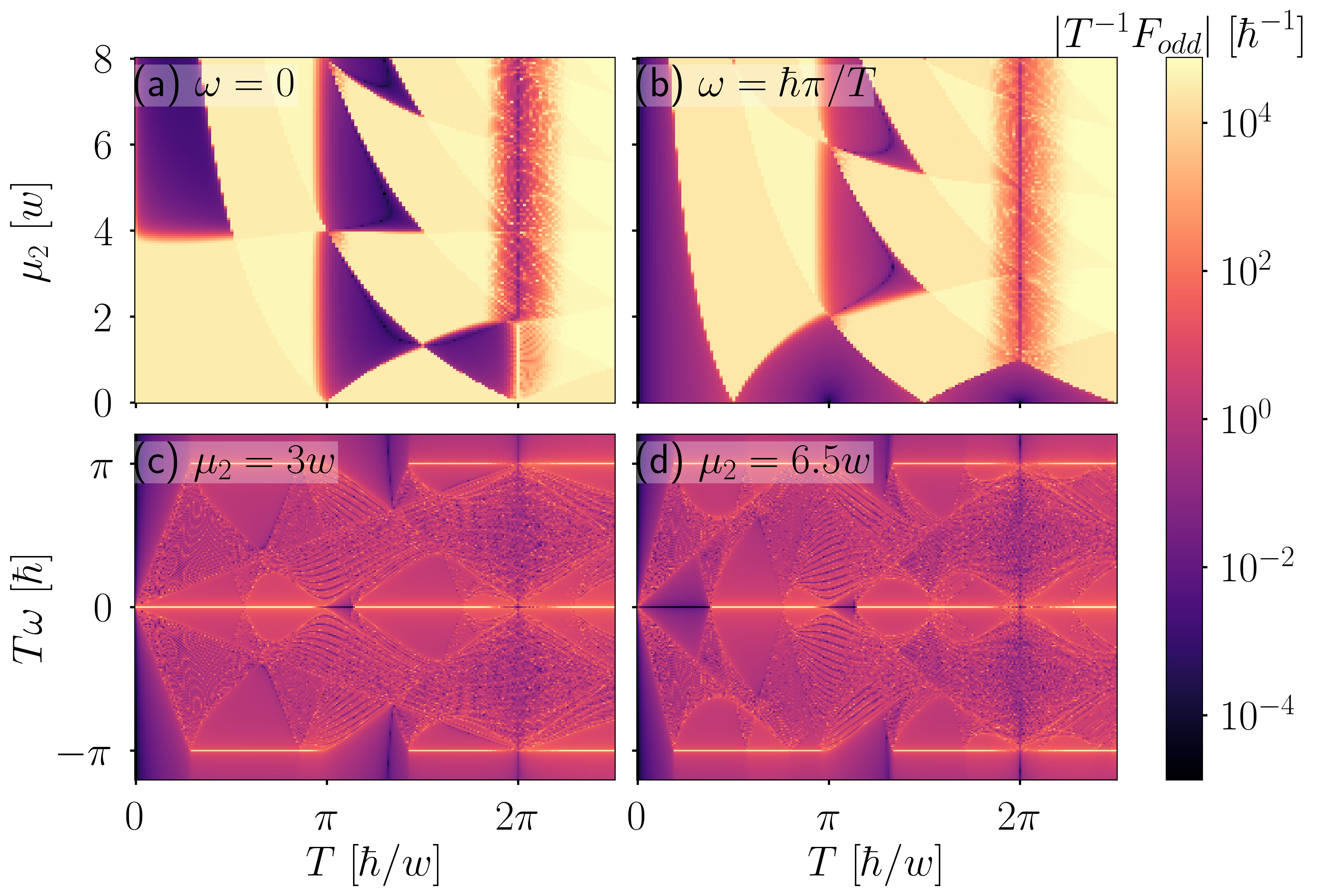
Figure 5: (a,b) Absolute value of the accumulated odd-frequency pair amplitude $F_{\rm odd}$ as a function of $\mu_{2}$ and $T$ for $\omega=0$ and $\omega=\pi\hbar/T$. (c,d) Same as in (a,b) but now as a function of $\omega$ and $T$ for $\mu_{2}=3w$ and $\mu_{2}=6.5w$. Parameters: $\Delta=w,\mu_{1}=0$, $N=100$, $\delta/w=10^{-5}$.

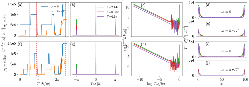
Figure 6: Absolute value of the accumulated odd-frequency pair amplitude $F_{\rm odd}$ as a function of $T$ (a,f), and $\omega$ (b,c,g,h). Panels (d,e,i,j) show the onsite odd-frequency pair amplitude $F_{ii}^{\rm odd}$ as a function of space $x$. The top and bottom rows correspond to $\mu_{2}=3w$ and $\mu_{2}=6.5w$, respectively. Parameters: $\Delta=w$, $\mu_{1}=0$, $N=100$.

Further insights on the relationship between Majorana modes and OTE pair correlations can be seen in Fig. 5(c,d) where we present $|F_{\rm odd}|$ as a function of $\omega$ and $T$. Interestingly, the odd-frequency pair amplitude exhibits its largest values at $\omega=0$ and $\omega=\pi\hbar/T$, which correspond to the quasienergies of MZMs and MPMs, respectively, discussed in Section III.3 and Fig. 4. This implies that the odd-frequency pairing resonates at the energies of the MZMs and MPMs, acquiring divergent frequency profiles that follow $\sim 1/\omega$ and $\sim 1/(\omega-\pi\hbar/T)$. This intriguing behaviour is confirmed in Fig. 6(b,g), where the odd-frequency pair amplitude $|F_{\rm odd}|$ is plotted as a function of $\omega$ at three fixed values of $T$. We also show ${\rm log}|T^{-1}\hbar F_{\rm odd}|$ in Fig. 6(c,h), which clearly reveals the divergent profile of $|F_{\rm odd}|$ at $\omega=0$ and $\omega=\pi\hbar/T$: here, the divergent peak at ${\rm log}|T\omega/\hbar\pi|=0$ depicts the divergence of the OTE pair amplitude at $\omega=\pi\hbar/T$, while the linear behavior shows that the OTE pair amplitude is also divergent when ${\rm log}|T\omega/\hbar\pi|$ takes large negative values which give at $\omega=0$ . The multiple peak structure appearing for ${\rm log}|T\omega/\hbar\pi|<0$ corresponds to contributions coming from the quasicontinuum of states seen in the dense regions of Fig. 4(a,b); they are, however, much smaller than OTE pairing due to MZMs and MPMs, as seen in Fig 6(b,g). Furthermore, we note that the OTE amplitude develops larger values when the number of MZMs or MPMs is larger, seen by noting the green, red and magenta colors in e.g., Fig. 6(b,g).

Having explored the frequency dependence of the OTE pair amplitude, next we inspect its real space dependence in order to gain even more understanding on its behaviour under the presence of Majorana modes. For this purpose, we address the odd-frequency pair amplitude before performing the summation in Eq. (14), namely, we inspect the real space profile of $F_{ii}^{\rm odd}$. This is visualized in Fig. 6(d,e,i,j), where we plot the absolute value of the OTE pair amplitude $|F_{ii}^{\rm odd}|$ as a function of $x=ia$ at $\omega=0$ (d,i) and $\omega=\pi\hbar/T$ (e,j); here the top and bottom rows correspond to $\mu_{2}=3w$ and $\mu_{2}=6.5w$, respectively. The main feature of the space dependence of the OTE pair amplitude is that they exhibit maxima at the edges of the system, in a very similar way as expected from the spatial nonlocal wavefunctions of Majorana edge modes. The accumulation of large OTE pair correlations at the edges is a well established effect in the static regime of topological superconductors, which reinforces the strong connection between MZMs and OTE pairing [2, 21, 67, 23, 24]. Our findings therefore reveal that the relationship between odd-frequency pairing and topology also holds for driven superconductors containing multiple MZMs and MPMs. In consequence, the nature of the emergent superconducting pairs at the boundaries of time-periodic topological superconductors is of OTE symmetry.

IV.2 Characterization of topology by the odd-frequency pairing amplitude

So far we have seen that there is an intriguing relationship between the emergence of Majorana edge states and odd-frequency pairing with OTE symmetry in time-periodic topological superconductors. Here we further investigate that this relationship is not accidental but it stems from the so-called spectral bulk boundary correspondence (SBBC), which predicts that the bulk winding number is related to odd-frequency pairing at boundaries in chiral symmetric systems [27, 70, 71]. The SBBC was studied before in chiral symmetric static systems and here we explore it in time-periodic domain.

We inspect the accumulated odd-frequency pairing $F_{\rm odd}$ defined in Eq. (14) with $t_{0}=T/4$. For this purpose we denote $F_{\rm odd}^{\rm N}(z)\equiv F_{\rm odd}(z)$ and write

$$F_{\rm odd}^{\rm N}(z)=\sum_{i}^{N/2}F_{ii}^{\rm odd}=\frac{1}{2}{\rm\hat{T}r}\{\Gamma G(z)\}\,,$$ (15)

where $\Gamma=\tau_{x}$ is the chiral operator, $G(z)=(z-H_{\rm F})^{-1}$ is the Green’s function, ${\rm\hat{T}r}$ represents a special trace operation that sums up the contributions from the leftmost lattice sites up to the middle of the system only, and $z$ represents complex frequencies, whose analytic continuation $z\rightarrow\omega\pm i\delta$ gives the advanced (retarded) Green’s functions studied in Eq. (14).

Then, taking $N$ very large such that the system becomes semi-infinity, in the low-frequency limit we find,

$$\lim_{N\rightarrow\infty}F_{\rm odd}^{\rm N}(z)=\frac{1}{2}\frac{W_{\omega}}{z-E_{\omega}}\,,$$ (16)

where $W_{\omega}$ corresponds to the winding numbers $W_{0(\pi)}$ obtained from Eq. (9), respectively. Moreover, $E_{\omega}$ corresponds to energies $E_{0}=0$ and $E_{\pi}=\pi\hbar/T$ of MZMs and MPMs, respectively. The accumulated odd-frequency pairing in Eq. (16) diverges at energies of MZMs or MPMs, in agreement with what we found in Fig. 6(b,c,g,h). Eq. (16) clearly demonstrates the direct relationship between odd-frequency pairing and topology in time-periodic topological superconductors. Also, it is worth noting that Eq. (16) extends the SBBC at low frequencies, initially investigated for static systems [27, 70, 71], to the time-dependent domain.

V Conclusions

In conclusion, we considered a one-dimensional $p$-wave superconductor under a time periodic chemical potential and studied the relationship between the emergence of Majorana edge modes and odd-frequency pairing. We found that Majorana modes appear located not only at energy $E_{\rm F}=0$, but also at $E_{\rm F}=\pi\hbar/T$, and, interestingly, the number of such Majorana edge modes can be controlled by the driving period and chemical potentials. Moreover, we discovered that odd-frequency pairing is finite and acquires large values in the presence of Majorana edge zero and $\pi$ modes, representing a unique out-of equilibrium phenomenon that can be fully controlled by the drive. Specially, we found that the frequency dependence of the formed odd-frequency pairing in the presence of Majorana zero and $\pi$ edge modes is proportional to $\sim 1/\omega$ and $\sim 1/(\omega-\pi\hbar/T)$, respectively. Moreover, we showed that the divergent profile of odd-frequency pairing remains even in the presence of multiple Majorana edge modes. Our results thus establish an intimately relationship between Majorana modes and odd-frequency pairing in time-driven topological superconductors.

VI Acknowledgements

We thank S. Ikegaya and Y. Kawaguchi for insightful discussions. E. A. acknowledges financial support from Nagoya University and Mitsubishi Foundation. S. T. thanks the support of the Würzburg-Dresden Cluster of Excellence ct.qmat, EXC2147, project-id 390858490, the DFG (SFB 1170), and the Bavarian Ministry of Economic Affairs, Regional Development and Energy within the High-Tech Agenda Project “Bausteine für das Quanten Computing auf Basis topologischer Materialen”. Y. T. acknowledges support from JSPS with Grants-in-Aid for Scientific research (KAKENHI Grants No. 23K17668 and 24K00583). J. C. acknowledges financial support from the Japan Society for the Promotion of Science via the International Research Fellow Program, the Swedish Research Council (Vetenskapsrådet Grant No. 2021-04121), and the Carl Trygger’s Foundation (Grant No. 22: 2093).

Appendix A Bulk quasienergy and bulk gaps

In this part we derive the bulk quasienergy given by Eq. (6), which is the key ingredient to obtain the gaps $g_{0,\pi}$ in Eqs. (10). For convenience, without loss of generality, we set $t_{0}=0$ in Eq. (4) and write the one-period propagator in momentum space in the following form

$$U_{T}=e^{-i\frac{T}{2\hbar}\bm{E}_{2}\cdot\bm{\tau}}e^{-i\frac{T}{2\hbar}\bm{E}_{1}\cdot\bm{\tau}}\,,$$ (17)

with $\bm{E}_{j}=(0,2\Delta\sin{k},-\mu_{j}-2w\cos{k})^{T}$ and $\bm{\tau}=(\tau_{x},\tau_{y},\tau_{z})$ the vector of Pauli matrices in Nambu space. As we see, the one-period propagator is expressed as a product of exponentials of Pauli matrices, which implies that it should follow the group composition law of $SU(2)$, i.e., it can be written as an exponential of $\mathfrak{su}(2)$ algebra. Thus, using Euler’s formula for Pauli matrices, we can write Eq. (17) as

$$\begin{split}U_{T}&=\mathbb{1}\Bigg{[}\cos\frac{E_{1}T}{2\hbar}\cos\frac{E_{2}T}{2\hbar}-\hat{E}_{1}\cdot\hat{E}_{2}\sin\frac{E_{1}T}{2\hbar}\sin\frac{E_{2}T}{2\hbar}\Bigg{]}\\ &+i\Bigg{[}\hat{E}_{1}\sin\frac{E_{1}T}{2\hbar}\cos\frac{E_{2}T}{2\hbar}+\hat{E}_{2}\sin\frac{E_{2}T}{2\hbar}\cos\frac{E_{1}T}{2\hbar}+\hat{E}_{1}\times\hat{E}_{2}\ \sin\frac{E_{1}T}{2\hbar}\sin\frac{E_{2}T}{2\hbar}\Bigg{]}\cdot\bm{\tau}\,,\end{split}$$ (18)

where $\hat{E}_{j}={\bm{E}_{j}}/{E_{j}},E_{j}=|{\bm{E}}_{j}|$, and ${\bm{E}}_{j}$ is defined below Eq. (17). Then, we use the fact that bulk quasienergies are eigenvalues of the eigenvalue problem defined by $U_{\rm T}\ket{\psi}=e^{-i\frac{T}{\hbar}H_{\rm F}(k)}\ket{\psi}$, where $H_{\rm F}(k)=\bm{E}_{\rm F}\cdot\bm{\tau}$. Thus,

$$e^{-i\frac{T}{\hbar}H_{\rm F}(k)}=\mathbb{1}\cos\frac{E_{F}T}{\hbar}+i\hat{E}_{F}\cdot\bm{\tau}\sin\frac{E_{F}T}{\hbar}\,,$$ (19)

At this point, we equate the Eq. (18) and Eq. (19), and, by comparing their terms proportional to the identity, we find that the Floquet quasienergy is given by

$$\begin{split}E_{\rm F}(k)&=\frac{\hbar}{T}\arccos[\cos(E_{1}T/2\hbar)\cos(E_{2}T/2\hbar)\\ \hfil&-\frac{\bm{E}_{1}\cdot\bm{E}_{2}}{E_{1}E_{2}}\sin(E_{1}T/2\hbar)\sin(E_{2}T/2\hbar)\bigg{]}\,.\end{split}$$ (20)

This is the Floquet bulk quasienergy presented in Eq. (6) of Subsection  III.3. Moreover, this quasienergy is then used to calculate the bulk gaps following Eq. (10) in the same Subsection. We note that the expression given by Eq. (20) is general as long as the one-period propagator takes the form of Eq. (17), suggesting its usefulness in other time-periodic systems.

One particular point here is that, at $k=\pi$, Eq. (20) transforms into ${\rm cos}[TE_{f}/\hbar]={\rm cos}[T(E_{1}+E_{2})/(2\hbar)]={\rm cos}[T(|-\mu_{1}+2w|+|-\mu_{2}+2w|)/(2\hbar)]$. Then, for $\mu_{1}+\mu_{2}=4w$, we get ${\rm cos}[TE_{f}/\hbar]=1$, which gives quasienergies equal to $E_{\rm F}=(2\pi n)\hbar/T$ for $n\in\mathbb{Z}$. Hence, for $n=0$, the quasienergy vanishes $E_{\rm F}=0$, which can be seen as a gap closing feature coming from the undriven phase because it happens at $\mu_{1}+\mu_{2}=4w$ which is the topological phase transition in the undriven regime where the system is described by $(H_{1}+H_{2})/2$. This gap closing is discussed in Subsection III.3.

Appendix B Baker-Campbell-Hausdorff expansion of the Floquet Hamiltonian

In this part we discuss the expansion of the Floquet Hamiltonian $H_{\rm F}$ given by Eq. (5) in terms of the driving period $T$. This is of particular relevance to understand the topological phase transition at $T=0$ and also the emergence of multiple Majorana modes due to long range hopping, both in Sec III. For this purpose, we fix $t_{0}=0$ without loss of generality and perform a Baker-Campbell-Hausdorff expansion of $H_{\rm F}$ up to third order in $T$, obtaining

$$H_{\rm F}(k)=\sum_{j=1}^{\infty}h_{j}\left(\frac{T}{\hbar}\right)^{j-1},$$ (21)

where

$$\begin{split}h_{1}&=\frac{1}{2}(H_{1}+H_{2})\\ &=-[(\mu_{1}+\mu_{2})/2+2w\cos(k)]\tau_{z}-2\Delta\sin(k)\tau_{y}\,,\\ h_{2}&=\frac{1}{2}\frac{1}{2^{2}}[H_{1},H_{2}]\\ &=\frac{i}{2}\Delta(-\mu_{1}+\mu_{2})\sin(k)\tau_{x}\,,\\ h_{3}&=\frac{1}{12}\frac{1}{2^{3}}([H_{1},[H_{1},H_{2}]]+[H_{2},[H_{2},H_{1}]])\\ &=\frac{-1}{12}\Delta{(\mu_{1}-\mu_{2})}^{2}\sin(k)\tau_{y}\,,\\ h_{4}&=-\frac{1}{24}\frac{1}{2^{4}}[H_{2},[H_{1},[H_{1},H_{2}]]]\\ &=\frac{i}{24}\Delta(\mu_{1}-\mu_{2})\sin(k)\big{[}-2\Delta^{2}-\mu_{1}\mu_{2}-2w^{2}-2(\mu_{1}+\mu_{2})w\cos k+2(\Delta^{2}-w^{2})\cos(2k)\big{]}\tau_{x}\,,\end{split}$$ (22)

where $H_{1,2}$ are given by Eq. (3) while $\Delta$, $w$, and $\mu_{1,2}$ are the order parameter, hopping, and chemical potentials respectively, as discussed in Eqs. (1) and (2).

The first observation in Eqs. (22) is that lowest term (near $T=0$) is given by $h_{1}=(H_{1}+H_{2})/2$, implying that the phase transition at $T=0$ is given by $|\mu_{1}+\mu_{2}|/2=2w$. Hence, for $\mu_{1}=0$, the topological phase transition is given by $|\mu_{2}|=4w$ as we indeed obtain in Subsection III.2 and Fig. 3. The second observation is the emergence of momentum dependent terms proportional to $[{\rm sin}(2k)]\tau_{x}$ and $[{\rm sin}(k){\rm cos}(2k)]\tau_{x}$ in the fourth order correction $h_{4}$. Thus, when performing a Fourier transformation to real space, these elements give rise to longer range pairing (next-nearest neighbor and second-next-nearest neighbor), which is used to argue the emergence of multiple Majorana modes in Subsection III.3. By adding more orders in the expansion, it is possible to also see the emergence of long range hopping.

References

- Qi and Zhang [2011] X.-L. Qi and S.-C. Zhang, Topological insulators and superconductors, Rev. Mod. Phys. 83, 1057 (2011).
- Tanaka et al. [2012] Y. Tanaka, M. Sato, and N. Nagaosa, Symmetry and topology in superconductors–odd-frequency pairing and edge states–, J. Phys. Soc. Japan 81, 011013 (2012).
- Leijnse and Flensberg [2012] M. Leijnse and K. Flensberg, Introduction to topological superconductivity and Majorana fermions, Semicond. Sci. Technol. 27, 124003 (2012).
- Beenakker [2013] C. Beenakker, Search for Majorana fermions in superconductors, Annu. Rev. Condens. Matter Phys. 4, 113 (2013).
- Sato and Ando [2017] M. Sato and Y. Ando, Topological superconductors: a review, Rep. Prog. Phys. 80, 076501 (2017).
- Sarma et al. [2015] S. D. Sarma, M. Freedman, and C. Nayak, Majorana zero modes and topological quantum computation, npj Quantum Inf. 1, 15001 (2015).
- Lahtinen and Pachos [2017] V. Lahtinen and J. K. Pachos, A Short Introduction to Topological Quantum Computation, SciPost Phys. 3, 021 (2017).
- Beenakker [2020] C. W. J. Beenakker, Search for non-Abelian Majorana braiding statistics in superconductors, SciPost Phys. Lect. Notes , 15 (2020).
- Aguado and Kouwenhoven [2020] R. Aguado and L. P. Kouwenhoven, Majorana qubits for topological quantum computing, Physics today 73, 44 (2020).
- Aguado [2020] R. Aguado, A perspective on semiconductor-based superconducting qubits, Appl. Phys. Lett. 117, 10.1063/5.0024124 (2020).
- Marra [2022] P. Marra, Majorana nanowires for topological quantum computation, J. Appl. Phys. 132, 231101 (2022).
- Lutchyn et al. [2018] R. M. Lutchyn, E. P. Bakkers, L. P. Kouwenhoven, P. Krogstrup, C. M. Marcus, and Y. Oreg, Majorana zero modes in superconductor–semiconductor heterostructures, Nat. Rev. Mater. 3, 52 (2018).
- Zhang et al. [2019] H. Zhang, D. E. Liu, M. Wimmer, and L. P. Kouwenhoven, Next steps of quantum transport in Majorana nanowire devices, Nat. Commun. 10, 5128 (2019).
- Prada et al. [2020] E. Prada, P. San-Jose, M. W. de Moor, A. Geresdi, E. J. Lee, J. Klinovaja, D. Loss, J. Nygård, R. Aguado, and L. P. Kouwenhoven, From Andreev to Majorana bound states in hybrid superconductor–semiconductor nanowires, Nat. Rev. Phys. 2, 575 (2020).
- Frolov et al. [2020] S. M. Frolov, M. J. Manfra, and J. D. Sau, Topological superconductivity in hybrid devices, Nat. Phys. 16, 718 (2020).
- Flensberg et al. [2021] K. Flensberg, F. von Oppen, and A. Stern, Engineered platforms for topological superconductivity and Majorana zero modes, Nat. Rev. Mater. 6, 944 (2021).
- Cayao et al. [2015] J. Cayao, E. Prada, P. San-Jose, and R. Aguado, SNS junctions in nanowires with spin-orbit coupling: Role of confinement and helicity on the subgap spectrum, Phys. Rev. B 91, 024514 (2015).
- Cayao and Burset [2021] J. Cayao and P. Burset, Confinement-induced zero-bias peaks in conventional superconductor hybrids, Phys. Rev. B 104, 134507 (2021).
- Tanaka et al. [2007] Y. Tanaka, Y. Tanuma, and A. A. Golubov, Odd-frequency pairing in normal-metal/superconductor junctions, Phys. Rev. B 76, 054522 (2007).
- Tanaka and Tamura [2018] Y. Tanaka and S. Tamura, Surface Andreev bound states and odd-frequency pairing in topological superconductor junctions, J. Low Temp. Phys. 191, 61 (2018).
- Cayao et al. [2020] J. Cayao, C. Triola, and A. M. Black-Schaffer, Odd-frequency superconducting pairing in one-dimensional systems, Eur. Phys. J. Special Topics 229, 545 (2020).
- Linder and Balatsky [2019] J. Linder and A. V. Balatsky, Odd-frequency superconductivity, Rev. Mod. Phys. 91, 045005 (2019).
- Tanaka and Tamura [2021] Y. Tanaka and S. Tamura, Theory of surface Andreev bound states and odd-frequency pairing in superconductor junctions, J. Supercond. Nov. Magn. 34, 1677 (2021).
- Tanaka et al. [2024] Y. Tanaka, S. Tamura, and J. Cayao, Theory of Majorana zero modes in unconventional superconductors (2024), arXiv:2402.00643 [cond-mat.supr-con] .
- Tanaka and Kashiwaya [2004] Y. Tanaka and S. Kashiwaya, Anomalous charge transport in triplet superconductor junctions, Phys. Rev. B 70, 012507 (2004).
- Takagi et al. [2020] D. Takagi, S. Tamura, and Y. Tanaka, Odd-frequency pairing and proximity effect in kitaev chain systems including a topological critical point, Phys. Rev. B 101, 024509 (2020).
- Tamura et al. [2019] S. Tamura, S. Hoshino, and Y. Tanaka, Odd-frequency pairs in chiral symmetric systems: Spectral bulk-boundary correspondence and topological criticality, Phys. Rev. B 99, 184512 (2019).
- Tsintzis et al. [2019] A. Tsintzis, A. M. Black-Schaffer, and J. Cayao, Odd-frequency superconducting pairing in kitaev-based junctions, Phys. Rev. B 100, 115433 (2019).
- Kuzmanovski et al. [2020] D. Kuzmanovski, A. M. Black-Schaffer, and J. Cayao, Suppression of odd-frequency pairing by phase disorder in a nanowire coupled to Majorana zero modes, Phys. Rev. B 101, 094506 (2020).
- Tamura and Tanaka [2019] S. Tamura and Y. Tanaka, Theory of the proximity effect in two-dimensional unconventional superconductors with rashba spin-orbit interaction, Phys. Rev. B 99, 184501 (2019).
- Yokoyama [2012] T. Yokoyama, Josephson and proximity effects on the surface of a topological insulator, Phys. Rev. B 86, 075410 (2012).
- Black-Schaffer and Balatsky [2012] A. M. Black-Schaffer and A. V. Balatsky, Odd-frequency superconducting pairing in topological insulators, Phys. Rev. B 86, 144506 (2012).
- Black-Schaffer and Balatsky [2013] A. M. Black-Schaffer and A. V. Balatsky, Proximity-induced unconventional superconductivity in topological insulators, Phys. Rev. B 87, 220506 (2013).
- Burset et al. [2015] P. Burset, B. Lu, G. Tkachov, Y. Tanaka, E. M. Hankiewicz, and B. Trauzettel, Superconducting proximity effect in three-dimensional topological insulators in the presence of a magnetic field, Phys. Rev. B 92, 205424 (2015).
- Lu et al. [2015] B. Lu, P. Burset, K. Yada, and Y. Tanaka, Tunneling spectroscopy and josephson current of superconductor-ferromagnet hybrids on the surface of a 3d TI, Supercond. Sci. Technol. 28, 105001 (2015).
- Crépin et al. [2015] F. Crépin, P. Burset, and B. Trauzettel, Odd-frequency triplet superconductivity at the helical edge of a topological insulator, Phys. Rev. B 92, 100507 (2015).
- Cayao and Black-Schaffer [2017] J. Cayao and A. M. Black-Schaffer, Odd-frequency superconducting pairing and subgap density of states at the edge of a two-dimensional topological insulator without magnetism, Phys. Rev. B 96, 155426 (2017).
- Kuzmanovski and Black-Schaffer [2017] D. Kuzmanovski and A. M. Black-Schaffer, Multiple odd-frequency superconducting states in buckled quantum spin hall insulators with time-reversal symmetry, Phys. Rev. B 96, 174509 (2017).
- Lu and Tanaka [2018] B. Lu and Y. Tanaka, Study on green’s function on topological insulator surface, Phil. Trans. R. Soc. A 376, 20150246 (2018).
- Keidel et al. [2018] F. Keidel, P. Burset, and B. Trauzettel, Tunable hybridization of Majorana bound states at the quantum spin hall edge, Phys. Rev. B 97, 075408 (2018).
- Breunig et al. [2018] D. Breunig, P. Burset, and B. Trauzettel, Creation of spin-triplet cooper pairs in the absence of magnetic ordering, Phys. Rev. Lett. 120, 037701 (2018).
- Fleckenstein et al. [2018] C. Fleckenstein, N. T. Ziani, and B. Trauzettel, Conductance signatures of odd-frequency superconductivity in quantum spin hall systems using a quantum point contact, Phys. Rev. B 97, 134523 (2018).
- Schmidt et al. [2020] J. Schmidt, F. Parhizgar, and A. M. Black-Schaffer, Odd-frequency superconductivity and meissner effect in the doped topological insulator , Phys. Rev. B 101, 180512 (2020).
- Cayao et al. [2022] J. Cayao, P. Dutta, P. Burset, and A. M. Black-Schaffer, Phase-tunable electron transport assisted by odd-frequency cooper pairs in topological josephson junctions, Phys. Rev. B 106, L100502 (2022).
- Dutta and Black-Schaffer [2019] P. Dutta and A. M. Black-Schaffer, Signature of odd-frequency equal-spin triplet pairing in the josephson current on the surface of weyl nodal loop semimetals, Phys. Rev. B 100, 104511 (2019).
- Parhizgar and Black-Schaffer [2020] F. Parhizgar and A. M. Black-Schaffer, Large josephson current in weyl nodal loop semimetals due to odd-frequency superconductivity, npj Quantum Materials 5, 42 (2020).
- Asano and Tanaka [2013] Y. Asano and Y. Tanaka, Majorana fermions and odd-frequency cooper pairs in a normal-metal nanowire proximity-coupled to a topological superconductor, Phys. Rev. B 87, 104513 (2013).
- Ebisu et al. [2016] H. Ebisu, B. Lu, J. Klinovaja, and Y. Tanaka, Theory of time-reversal topological superconductivity in double Rashba wires: symmetries of cooper pairs and Andreev bound states, Prog. Theor. Exp. Phys. 2016, 083I01 (2016).
- Cayao and Black-Schaffer [2018] J. Cayao and A. M. Black-Schaffer, Odd-frequency superconducting pairing in junctions with Rashba spin-orbit coupling, Phys. Rev. B 98, 075425 (2018).
- Lee et al. [2017] S.-P. Lee, R. M. Lutchyn, and J. Maciejko, Odd-frequency superconductivity in a nanowire coupled to Majorana zero modes, Phys. Rev. B 95, 184506 (2017).
- Gnezdilov [2019] N. V. Gnezdilov, Gapless odd-frequency superconductivity induced by the sachdev-ye-kitaev model, Phys. Rev. B 99, 024506 (2019).
- Huang et al. [2015] Z. Huang, P. Wölfle, and A. V. Balatsky, Odd-frequency pairing of interacting Majorana fermions, Phys. Rev. B 92, 121404 (2015).
- Golubov et al. [2009] A. A. Golubov, Y. Tanaka, Y. Asano, and Y. Tanuma, Odd-frequency pairing in superconducting heterostructures, J. Phys.: Condens. Matter 21, 164208 (2009).
- Balatsky et al. [2020] A. V. Balatsky, P. O. Sukhachov, and S. Bandyopadhyay, Quantum pairing time orders, Annalen der Physik 532, 1900529 (2020).
- Jiang et al. [2011] L. Jiang, T. Kitagawa, J. Alicea, A. R. Akhmerov, D. Pekker, G. Refael, J. I. Cirac, E. Demler, M. D. Lukin, and P. Zoller, Majorana fermions in equilibrium and in driven cold-atom quantum wires, Phys. Rev. Lett. 106, 220402 (2011).
- Goldman and Dalibard [2014] N. Goldman and J. Dalibard, Periodically driven quantum systems: Effective hamiltonians and engineered gauge fields, Phys. Rev. X 4, 031027 (2014).
- Bukov et al. [2015] M. Bukov, L. D’Alessio, and A. Polkovnikov, Universal high-frequency behavior of periodically driven systems: from dynamical stabilization to floquet engineering, Advances in Physics 64, 139 (2015).
- Asbóth and Obuse [2013] J. K. Asbóth and H. Obuse, Bulk-boundary correspondence for chiral symmetric quantum walks, Phys. Rev. B 88, 121406 (2013).
- Asbóth et al. [2014] J. K. Asbóth, B. Tarasinski, and P. Delplace, Chiral symmetry and bulk-boundary correspondence in periodically driven one-dimensional systems, Phys. Rev. B 90, 125143 (2014).
- Wu et al. [2023] H. Wu, S. Wu, and L. Zhou, Floquet topological superconductors with many Majorana edge modes: topological invariants, entanglement spectrum and bulk-edge correspondence, New J. Phys. 25, 083042 (2023).
- DeGottardi et al. [2013] W. DeGottardi, M. Thakurathi, S. Vishveshwara, and D. Sen, Majorana fermions in superconducting wires: Effects of long-range hopping, broken time-reversal symmetry, and potential landscapes, Phys. Rev. B 88, 165111 (2013).
- Tong et al. [2013] Q.-J. Tong, J.-H. An, J. Gong, H.-G. Luo, and C. H. Oh, Generating many Majorana modes via periodic driving: A superconductor model, Phys. Rev. B 87, 201109 (2013).
- Zhou [2020] L. Zhou, Non-hermitian floquet topological superconductors with multiple Majorana edge modes, Phys. Rev. B 101, 014306 (2020).
- Zhou [2022] L. Zhou, Generating many Majorana corner modes and multiple phase transitions in floquet second-order topological superconductors, Symmetry 14, 10.3390/sym14122546 (2022).
- Zagoskin [1998] A. M. Zagoskin, Quantum theory of many-body systems, Vol. 174 (Springer, 1998).
- Mahan [2013] G. D. Mahan, Many-particle physics (Springer Science & Business Media, 2013).
- Triola et al. [2020] C. Triola, J. Cayao, and A. M. Black-Schaffer, The role of odd-frequency pairing in multiband superconductors, Ann. Phys. 532, 1900298 (2020).
- Tanaka and Golubov [2007] Y. Tanaka and A. A. Golubov, Theory of the proximity effect in junctions with unconventional superconductors, Phys. Rev. Lett. 98, 037003 (2007).
- Note [1] For , which is roughly the leftmost value of the axis in Fig.\tmspace+.1667em6(c,h), we obtain and , thus revealing the enhancement of the OTE amplitude at zero energy.
- Daido and Yanase [2019] A. Daido and Y. Yanase, Chirality polarizations and spectral bulk-boundary correspondence, Phys. Rev. B 100, 174512 (2019).
- Tamura et al. [2020] S. Tamura, S. Nakosai, A. M. Black-Schaffer, Y. Tanaka, and J. Cayao, Bulk odd-frequency pairing in the superconducting Su-Schrieffer-Heeger model, Phys. Rev. B 101, 214507 (2020).