Computation and analysis of subdiffusion with variable exponent

Abstract

We consider the subdiffusion of variable exponent modeling subdiffusion phenomena with varying memory properties. The main difficulty is that this model could not be analytically solved and the variable-exponent Abel kernel may not be positive definite or monotonic. This work develops a tool called the generalized identity function to convert this model to more feasible formulations for mathematical and numerical analysis, based on which we prove its well-posedness and regularity. In particular, we characterize the singularity of the solutions in terms of the initial value of the exponent. Then the semi-discrete and fully-discrete numerical methods are developed and their error estimates are proved, without any regularity assumption on solutions or requiring specific properties of the variable-exponent Abel kernel. The convergence order is also characterized by the initial value of the exponent. Finally, we investigate an inverse problem of determining the initial value of the exponent.

1 Introduction

We consider the subdiffusion model with variable exponent, which has been used in various fields such as the transient dispersion in heterogeneous media [26, 27, 30, 32]

$$\begin{array}[]{c}(k*\partial_{t}u)(\bm{x},t)-\Delta u(\bm{x},t)=f(\bm{x},t),~{}~{}(\bm{x},t)\in\Omega\times(0,T],\end{array}$$ (1)

equipped with initial and boundary conditions

$$u(\bm{x},0)=u_{0}(\bm{x}),~{}\bm{x}\in\Omega;\quad u(\bm{x},t)=0,~{}(\bm{x},t)\in\partial\Omega\times[0,T].$$ (2)

Here $\Omega\subset\mathbb{R}^{d}$ is a simply-connected bounded domain with the piecewise smooth boundary $\partial\Omega$ with convex corners, $\bm{x}:=(x_{1},\cdots,x_{d})$ with $1\leq d\leq 3$ denotes the spatial variables, $f$ and $u_{0}$ refer to the source term and the initial value, respectively, and the fractional derivative of order $0<\alpha(t)<1$ is defined via the variable-exponent Abel kernel $k$ [18]

$$(k*\partial_{t}u)(\bm{x},t):=\int_{0}^{t}k(t-s)\partial_{s}u(\bm{x},s)ds,~{}~{}k(t):=\frac{t^{-\alpha(t)}}{\Gamma(1-\alpha(t))}.$$

There exist extensive investigations and significant progresses for the constant exponent case $\alpha(t)\equiv\alpha$ of subdiffusion model (1)–(2) [3, 8, 10, 13, 15, 16, 17], while much fewer investigations for the variable exponent case can be found in the literature. There exist some mathematical and numerical results on model (1)–(2) with space-variable-dependent variable exponent [12, 14, 31]. For the time-variable-dependent case, there are some recent works changing the exponent in the Laplace domain [4, 6] such that the Laplace transform of the variable-exponent fractional operator is available. For the case that the exponent changes in the time domain, the only available results focus on the piecewise-constant variable exponent case such that the solution representation is available on each temporal piece [11, 29]. It is also commented in [11] that the case of continuously varying exponent remains an open problem, which motivates the current study.

The main difficulty for investigating the case of continuously varying exponent is that the model (1)–(2) could not be analytically solved and the variable-exponent Abel kernel may not be positive definite or monotonic. To circumvent this issue, we develop a tool called the generalized identity function to convert this model to more feasible formulations, based on which we prove its well-posedness and regularity by means of resolvent estimates. In particular, we characterize the singularity of the solutions in terms of the initial value $\alpha(0)$ of the exponent, which indicates an intrinsic factor of variable-exponent models. Then the semi-discrete and fully-discrete numerical methods are developed and their error estimates are proved, without any regularity assumption on solutions or requiring specific properties of the variable-exponent Abel kernel such as positive definiteness or monotonicity. We again characterize the convergence order by $\alpha(0)$. Since the $\alpha(0)$ plays a critical role in characterizing properties of the model and the numerical method, we present a preliminary result for the inverse problem of determining $\alpha(0)$. Based on the idea of the generalized identity function and the developed techniques, one could further investigate different kinds of variable-exponent fractional problems that will be considered in the future.

The rest of the work is organized as follows: In Section 2 we introduce notations and the generalization identity function. In Section 3 we prove the well-posedness of a transformed model, based on which we prove the well-posedness and regularity of the original model (1)–(2) in Section 4. In Section 5 we derive a numerically-feasible formulation and analyze its semi-discrete finite element scheme. In Section 6 a fully-discrete scheme with a second-order quadrature rule in time is proposed and analyzed. Numerical examples are performed in Section 7 for demonstration, and we address the inverse problem of determining $\alpha(0)$ in the last section.

2 Preliminaries

2.1 Notations

For the sake of clear presentation, we introduce the following spaces and notations. Let $L^{p}(\Omega)$ with $1\leq p\leq\infty$ be the Banach space of $p$th power Lebesgue integrable functions on $\Omega$. Denote the inner product of $L^{2}(\Omega)$ as $(\cdot,\cdot)$. For a positive integer $m$, let $W^{m,p}(\Omega)$ be the Sobolev space of $L^{p}$ functions with $m$th weakly derivatives in $L^{p}(\Omega)$ (similarly defined with $\Omega$ replaced by an interval $\mathcal{I}$). Let $H^{m}(\Omega):=W^{m,2}(\Omega)$ and $H^{m}_{0}(\Omega)$ be its subspace with the zero boundary condition up to order $m-1$. For a non-integer $s\geq 0$, $H^{s}(\Omega)$ is defined via interpolation [1]. Let $\{\lambda_{i},\phi_{i}\}_{i=1}^{\infty}$ be eigen-pairs of the problem $-\Delta\phi_{i}=\lambda_{i}\phi_{i}$ with the zero boundary condition. We introduce the Sobolev space $\check{H}^{s}(\Omega)$ for $s\geq 0$ by $\check{H}^{s}(\Omega):=\big{\{}q\in L^{2}(\Omega):\|q\|_{\check{H}^{s}}^{2}:=\sum_{i=1}^{\infty}\lambda_{i}^{s}(q,\phi_{i})^{2}<\infty\big{\}},$ which is a subspace of $H^{s}(\Omega)$ satisfying $\check{H}^{0}(\Omega)=L^{2}(\Omega)$ and $\check{H}^{2}(\Omega)=H^{2}(\Omega)\cap H^{1}_{0}(\Omega)$ [28]. For a Banach space $\mathcal{X}$, let $W^{m,p}(0,T;\mathcal{X})$ be the space of functions in $W^{m,p}(0,T)$ with respect to $\|\cdot\|_{\mathcal{X}}$. All spaces are equipped with standard norms [1, 5].

We use $Q$ to denote a generic positive constant that may assume different values at different occurrences. We use $\|\cdot\|$ to denote the $L^{2}$ norm of functions or operators in $L^{2}(\Omega)$, set $L^{p}(\mathcal{X})$ for $L^{p}(0,T;\mathcal{X})$ for brevity, and drop the notation $\Omega$ in the spaces and norms if no confusion occurs. For instance, $L^{2}(L^{2})$ implies $L^{2}(0,T;L^{2}(\Omega))$. Furthermore, we will drop the space variable $\bm{x}$ in functions, e.g. we denote $q(\bm{x},t)$ as $q(t)$, when no confusion occurs.

For $\theta\in(\pi/2,\pi)$ and $\delta>0$, let $\Gamma_{\theta}$ be the contour in the complex plane defined by $\Gamma_{\theta}:=\big{\{}z\in\mathbb{C}:|{\rm arg}(z)|=\theta,|z|\geq\delta\big{\}}\cup\big{\{}z\in\mathbb{C}:|{\rm arg}(z)|\leq\theta,|z|=\delta\big{\}}.$ For any $q\in L^{1}_{loc}(\mathcal{I})$, the Laplace transform $\mathcal{L}$ of its extension $\tilde{q}(t)$ to zero outside $\mathcal{I}$ and the corresponding inverse transform $\mathcal{L}^{-1}$ are denoted by

$$\mathcal{L}q(z):=\int_{0}^{\infty}\tilde{q}(t)e^{-tz}dt,\quad\mathcal{L}^{-1}(\mathcal{L}q(z)):=\frac{1}{2\pi\rm i}\int_{\Gamma_{\theta}}e^{tz}\mathcal{L}q(z)dz=q(t).$$

The following inequalities hold for $0<\mu<1$ and $Q=Q(\theta,\mu)$ [2, 19, 23]

$$\int_{\Gamma_{\theta}}|z|^{\mu-1}|e^{tz}|\,|dz|\leq Qt^{-\mu},~{}~{}t\in(0,T];~{}~{}\|(z^{\mu}-\Delta)^{-1}\|\leq Q|z|^{-\mu},~{}~{}\forall z\in\Gamma_{\theta},$$ (3)

and we have $\mathcal{L}(\partial_{t}^{\mu}q)=z^{\mu}\mathcal{L}q-(I_{t}^{1-\mu}q)(0)$ [9].

Throughout this work, we consider smooth $\alpha(t)$. Specifically, we assume $\alpha(t)$ is three times differentiable with $|\alpha^{\prime}(t)|+|\alpha^{\prime\prime}(t)|+|\alpha^{\prime\prime\prime}(t)|\leq L$ for some $L>0$. We also denote $\alpha_{0}=\alpha(0)$ for simplicity.

2.2 A generalized identity function

For $0<\mu<1$, define $\beta_{\mu}(t):=\frac{t^{\mu-1}}{\Gamma(\mu)}$ and the notations $I_{t}^{\mu}q:=\beta_{\mu}*q$ and $\partial_{t}^{\mu}q=\partial_{t}(\beta_{1-\mu}*q)$. Then direct calculation yields

$$(\beta_{\alpha_{0}}*k)(t)= \int_{0}^{t}\frac{(t-s)^{\alpha_{0}-1}}{\Gamma(\alpha_{0})}\frac{s^{-\alpha(s)}}{\Gamma(1-\alpha(s))}ds$$

$$\overset{z=s/t}{=}\int_{0}^{1}\frac{(t-tz)^{\alpha_{0}-1}}{\Gamma(\alpha_{0})}\frac{(tz)^{-\alpha(tz)}}{\Gamma(1-\alpha(tz))}tdz$$ (4)

$$=\int_{0}^{1}\frac{(tz)^{\alpha_{0}-\alpha(tz)}}{\Gamma(\alpha_{0})\Gamma(1-\alpha(tz))}(1-z)^{\alpha_{0}-1}z^{-\alpha_{0}}dz=:g(t).$$

It is clear that if $\alpha(t)\equiv\alpha$ for some constant $0<\alpha<1$, then $g(t)=\int_{0}^{1}\frac{1}{\Gamma(\alpha)\Gamma(1-\alpha)}(1-z)^{\alpha-1}z^{-\alpha}dz=1.$ For the variable exponent $\alpha(t)$, $g(t)\not\equiv 1$ in general. However, as

$$\lim_{t\rightarrow 0^{+}}|(\alpha_{0}-\alpha(tz))\ln tz|\leq\lim_{t\rightarrow 0^{+}}Ltz|\ln tz|=0,$$

we have $\lim_{t\rightarrow 0^{+}}(tz)^{\alpha_{0}-\alpha(tz)}=\lim_{t\rightarrow 0^{+}}e^{(\alpha_{0}-\alpha(tz))\ln tz}=1,$ which implies

$$g(0)=\int_{0}^{1}\frac{1}{\Gamma(\alpha_{0})\Gamma(1-\alpha_{0})}(1-z)^{\alpha_{0}-1}z^{-\alpha_{0}}dz=1.$$ (5)

Based on this property, we call $g(t)$ a generalized identity function, which will play a key role in reformulating the model (1) to more feasible forms for mathematical and numerical analysis.

It is clear that $g$ is bounded over $[0,T]$. To bound derivatives of $g$, we use $(tz)^{\alpha_{0}-\alpha(tz)}\leq Q$ to obtain

$$\Big{|}\partial_{t}(tz)^{\alpha_{0}-\alpha(tz)}\Big{|} =\Big{|}(tz)^{\alpha_{0}-\alpha(tz)}z\Big{(}-\alpha^{\prime}(tz)\ln(tz)+\frac{\alpha_{0}-\alpha(tz)}{tz}\Big{)}\Big{|}$$

$$\leq Qz\big{(}|\ln(tz)|+1\big{)},$$

$$\Big{|}\partial_{t}^{2}(tz)^{\alpha_{0}-\alpha(tz)}\Big{|} =\Big{|}\big{[}\partial_{t}(tz)^{\alpha_{0}-\alpha(tz)}\big{]}z\Big{(}-\alpha^{\prime}(tz)\ln(tz)+\frac{\alpha_{0}-\alpha(tz)}{tz}\Big{)}$$

$$\quad+(tz)^{\alpha_{0}-\alpha(tz)}z^{2}\Big{(}-\alpha^{\prime\prime}(tz)\ln(tz)-2\frac{\alpha^{\prime}(tz)}{tz}-\frac{\alpha_{0}-\alpha(tz)}{(tz)^{2}}\Big{)}\Big{|}$$

$$\leq Qz^{2}\big{(}|\ln(tz)|+1\big{)}^{2}+z^{2}(|\ln(tz)|+\frac{1}{tz})\leq Q\frac{z^{2}}{tz}=Q\frac{z}{t},$$

$$\Big{|}\partial_{t}^{3}(tz)^{\alpha_{0}-\alpha(tz)}\Big{|} \leq\frac{Q}{t^{2}}~{}(\text{We omit the calculations here}).$$

We apply them to bound $g^{\prime}(t)$, $g^{\prime\prime}(t)$ and $g^{\prime\prime\prime}(t)$ as

$$|g^{\prime}| =\Big{|}\int_{0}^{1}\partial_{t}\Big{(}\frac{(tz)^{\alpha_{0}-\alpha(tz)}}{\Gamma(\alpha_{0})\Gamma(1-\alpha(tz))}\Big{)}(1-z)^{\alpha_{0}-1}z^{-\alpha_{0}}dz\Big{|}$$

$$\leq Q\int_{0}^{1}z\big{(}|\ln(tz)|+1\big{)}(1-z)^{\alpha_{0}-1}z^{-\alpha_{0}}dz$$

$$\leq Q\big{(}|\ln t|+1\big{)}\int_{0}^{1}z\frac{|\ln t|+|\ln z|+1}{|\ln t|+1}(1-z)^{\alpha_{0}-1}z^{-\alpha_{0}}dz\leq Q\big{(}|\ln t|+1\big{)},$$ (6)

$$|g^{\prime\prime}| =\Big{|}\int_{0}^{1}\partial_{t}^{2}\Big{(}\frac{(tz)^{\alpha_{0}-\alpha(tz)}}{\Gamma(\alpha_{0})\Gamma(1-\alpha(tz))}\Big{)}(1-z)^{\alpha_{0}-1}z^{-\alpha_{0}}dz\Big{|}\leq\frac{Q}{t},$$ (7)

$$|g^{\prime\prime\prime}| =\Big{|}\int_{0}^{1}\partial_{t}^{3}\Big{(}\frac{(tz)^{\alpha_{0}-\alpha(tz)}}{\Gamma(\alpha_{0})\Gamma(1-\alpha(tz))}\Big{)}(1-z)^{\alpha_{0}-1}z^{-\alpha_{0}}dz\Big{|}\leq\frac{Q}{t^{2}}.$$ (8)

3 Auxiliary results

We propose a transformed model of (1)–(2) and then prove its well-posedness for future use.

3.1 A transformed model

We calculate the convolution of (1) and $\beta_{\alpha_{0}}$ as $\beta_{\alpha_{0}}*[(k*\partial_{t}u)-\Delta u-f]=0.$ We invoke (4) to obtain

$$g*\partial_{t}u-\beta_{\alpha_{0}}*\Delta u-\beta_{\alpha_{0}}*f=0.$$ (9)

We finally use (5) to formally differentiate it to get the transformed model

$$\partial_{t}u+g^{\prime}*\partial_{t}u-\partial_{t}^{1-\alpha_{0}}\Delta u=\partial_{t}^{1-\alpha_{0}}f,$$ (10)

equipped with the initial and boundary conditions (2).

We then take the Laplace transform of (10) to obtain

$$z\mathcal{L}u-u_{0}-z^{1-\alpha_{0}}\Delta\mathcal{L}u=\mathcal{L}p_{u},~{}~{}p_{u}(t):=\partial_{t}^{1-\alpha_{0}}f-g^{\prime}*\partial_{t}u,$$

that is, $\mathcal{L}u=z^{\alpha_{0}-1}(z^{\alpha_{0}}-\Delta)^{-1}(u_{0}+\mathcal{L}p_{u}).$ Take the inverse Laplace transform to get

$$u=F(t)u_{0}+\int_{0}^{t}F(t-s)p_{u}(s)ds$$ (11)

where the operator $F(\cdot):L^{2}(\Omega)\rightarrow L^{2}(\Omega)$ is defined as

$$F(t)q:=\frac{1}{2\pi\rm i}\int_{\Gamma_{\theta}}e^{tz}z^{\alpha_{0}-1}(z^{\alpha_{0}}-\Delta)^{-1}qdz,~{}~{}\forall q\in L^{2}(\Omega),$$

with the following properties [9]

$$\|F(t)q\|_{\check{H}^{\mu}}\leq Qt^{\frac{\gamma-\mu}{2}\alpha_{0}}\|q\|_{\check{H}^{\gamma}}\text{ for }\mu,\gamma\in\mathbb{R}\text{ and }\gamma\leq\mu\leq\gamma+2.$$ (12)

3.2 Well-posedness of transformed model

We show the well-posedness of model (10) with the initial and boundary conditions (2) in the following theorem.

Theorem 1.

Suppose $f\in W^{1,1}(L^{2})$ and $u_{0}\in\check{H}^{2}$, then model (10)–(2) admits a unique solution in $W^{1,p}(L^{2})\cap L^{p}(\check{H}^{2})$ for $1<p<\frac{1}{1-\alpha_{0}}$ and

$$\|u\|_{W^{1,p}(L^{2})}+\|u\|_{L^{p}(\check{H}^{2})}\leq Q\big{(}\|f\|_{W^{1,1}(L^{2})}+\|u_{0}\|_{\check{H}^{2}}\big{)}.$$

Proof.

By $C([0,T];L^{2})\subset W^{1,1}(L^{2})$ [1], we have the following relations for $0<\varepsilon\ll\frac{1}{p}-(1-\alpha_{0})$

$$I_{t}^{1-\varepsilon}\partial_{t}^{1-\alpha_{0}}f=I_{t}^{\alpha_{0}-\varepsilon}f,~{}~{}\partial_{t}^{\varepsilon}\partial_{t}^{1-\alpha_{0}}f=\beta_{\alpha_{0}-\varepsilon}f(0)+\beta_{\alpha_{0}-\varepsilon}*\partial_{t}f,$$ (13)

which means that

$$(I_{t}^{1-\varepsilon}\partial_{t}^{1-\alpha_{0}}f)|_{t=0}=0,~{}~{}\|\partial_{t}^{\varepsilon}\partial_{t}^{1-\alpha_{0}}f\|_{L^{p}(L^{2})}\leq Q\|f\|_{W^{1,1}(L^{2})}.$$ (14)

Thus we take $0<\varepsilon\ll\frac{1}{p}-(1-\alpha_{0})$ throughout this proof.

We first consider the case of zero initial condition, i.e. $u_{0}\equiv 0$, and define the space $\tilde{W}^{1,p}(L^{2}):=\{q\in W^{1,p}(L^{2}):q(0)=0\}$ equipped with the norm $\|q\|_{\tilde{W}^{1,p}(L^{2})}:=\|e^{-\sigma t}\partial_{t}q\|_{L^{p}(L^{2})}$ for some $\sigma\geq 1$, which is equivalent to the standard norm $\|q\|_{W^{1,p}(L^{2})}$ for $q\in\tilde{W}^{1,p}(L^{2})$. Define a mapping $\mathcal{M}:\tilde{W}^{1,p}(L^{2})\rightarrow\tilde{W}^{1,p}(L^{2})$ by $w=\mathcal{M}v$ where $w$ satisfies

$$\partial_{t}w-\partial_{t}^{1-\alpha_{0}}\Delta w=p_{v},~{}~{}(\bm{x},t)\in\Omega\times(0,T],$$ (15)

equipped with zero initial and boundary conditions. By (11), $w$ could be expressed as

$$w=\int_{0}^{t}F(t-s)p_{v}(s)ds.$$ (16)

To show the well-posedness of $\mathcal{M}$, we differentiate (16) to obtain

$$\partial_{t}w=p_{v}(t)+\int_{0}^{t}F^{\prime}(t-s)p_{v}(s)ds.$$ (17)

We use the Laplace transform to evaluate the second right-hand side term to get

$$\mathcal{L}\bigg{[}\int_{0}^{t}F^{\prime}(t-s)p_{v}(s)ds\bigg{]}=z^{\alpha_{0}}(z^{\alpha_{0}}-\Delta)^{-1}\mathcal{L}p_{v}=\big{(}z^{\alpha_{0}-\varepsilon}(z^{\alpha_{0}}-\Delta)^{-1}\big{)}\big{(}z^{\varepsilon}\mathcal{L}p_{v}\big{)}.$$ (18)

We apply $(I_{t}^{1-\varepsilon}\partial_{t}^{1-\alpha_{0}}f)(0)=0$ to take the inverse Laplace transform of (18) to get

$$\int_{0}^{t}F^{\prime}(t-s)p_{v}(s)ds=\int_{0}^{t}\mathcal{R}(t-s)\partial_{s}^{\varepsilon}p_{v}(s)ds,$$ (19)

where $\mathcal{R}(t):=\frac{1}{2\pi\rm i}\int_{\Gamma_{\theta}}z^{\alpha_{0}-\varepsilon}(z^{\alpha_{0}}-\Delta)^{-1}e^{zt}\mathrm{d}z.$ We use (3) to bound $\mathcal{R}$ by

$$\|\mathcal{R}(t-s)\| \leq Q\int_{\Gamma_{\theta}}|z|^{\alpha_{0}-\varepsilon}\|(z^{\alpha_{0}}-\Delta)^{-1}\||e^{z(t-s)}||dz|$$

$$\leq Q\int_{\Gamma_{\theta}}|z|^{\alpha_{0}-\varepsilon}|z|^{-\alpha_{0}}|e^{z(t-s)}||dz|\leq\frac{Q}{(t-s)^{1-\varepsilon}}.$$ (20)

To estimate $\partial_{t}^{\varepsilon}p_{v}$, recall that $p_{v}(t)=\partial_{t}^{1-\alpha_{0}}f-g^{\prime}*\partial_{t}v$, which implies

$$\partial_{t}^{\varepsilon}p_{v}(t)=\partial_{t}^{\varepsilon}\partial_{t}^{1-\alpha_{0}}f-\partial_{t}^{\varepsilon}(g^{\prime}*\partial_{t}v).$$ (21)

We reformulate $\partial_{t}^{\varepsilon}(g^{\prime}*\partial_{t}v)$ as

$$\partial_{t}^{\varepsilon}(g^{\prime}*\partial_{t}v)=\partial_{t}\big{(}\beta_{1-\varepsilon}*(g^{\prime}*\partial_{t}v)\big{)}=\partial_{t}\big{(}(\beta_{1-\varepsilon}*g^{\prime})*\partial_{t}v\big{)},$$ (22)

where

$$\beta_{1-\varepsilon}*g^{\prime}=\int_{0}^{t}\frac{(t-s)^{-\varepsilon}}{\Gamma(1-\varepsilon)}g^{\prime}(s)ds=t^{1-\varepsilon}\int_{0}^{1}\frac{(1-z)^{-\varepsilon}}{\Gamma(1-\varepsilon)}g^{\prime}(tz)dz.$$ (23)

By (6), we have

$$|\beta_{1-\varepsilon}*g^{\prime}| \leq Qt^{1-\varepsilon}\int_{0}^{1}\frac{(1-z)^{-\varepsilon}}{\Gamma(1-\varepsilon)}(1+|\ln(tz)|)dz$$

$$\leq Qt^{1-\varepsilon}\int_{0}^{1}(1-z)^{-\varepsilon}\frac{(tz)^{\varepsilon}(1+|\ln(tz)|)}{(tz)^{\varepsilon}}dz\leq Qt^{1-2\varepsilon},$$ (24)

which means that $(\beta_{1-\varepsilon}*g^{\prime})(0)=0$. We apply this to further rewrite (22) as

$$\partial_{t}^{\varepsilon}(g^{\prime}*\partial_{t}v)=\big{(}\partial_{t}(\beta_{1-\varepsilon}*g^{\prime})\big{)}*\partial_{t}v.$$ (25)

Based on (23) we apply (7) and a similar estimate as (24) to obtain

$$|\partial_{t}(\beta_{1-\varepsilon}*g^{\prime})| =\Big{|}(1-\varepsilon)t^{-\varepsilon}\int_{0}^{1}\frac{(1-z)^{-\varepsilon}}{\Gamma(1-\varepsilon)}g^{\prime}(tz)dz$$

$$\qquad+t^{1-\varepsilon}\int_{0}^{1}\frac{(1-z)^{-\varepsilon}}{\Gamma(1-\varepsilon)}g^{\prime\prime}(tz)zdz\Big{|}\leq Qt^{-2\varepsilon}.$$ (26)

Thus, we finally bound $\partial_{t}^{\varepsilon}(g^{\prime}*\partial_{t}v)$ as

$$|\partial_{t}^{\varepsilon}(g^{\prime}*\partial_{t}v)|\leq Qt^{-2\varepsilon}*|\partial_{t}v|.$$ (27)

We invoke (14) and (27) to conclude that

$$\|e^{-\sigma t}\partial_{t}^{\varepsilon}p_{v}(t)\|_{L^{p}(L^{2})} \leq\|\partial_{t}^{\varepsilon}\partial_{t}^{1-\alpha_{0}}f\|_{L^{p}(L^{2})}+Q\|e^{-\sigma t}(t^{-2\varepsilon}*|\partial_{t}v|)\|_{L^{p}(L^{2})}$$

$$\leq\|f\|_{W^{1,1}(L^{2})}+Q\|(e^{-\sigma t}t^{-2\varepsilon})*(e^{-\sigma t}\|\partial_{t}v\|)\|_{L^{p}(0,T)}$$

$$\leq\|f\|_{W^{1,1}(L^{2})}+Q\|e^{-\sigma t}t^{-2\varepsilon}\|_{L^{1}(0,T)}\|e^{-\sigma t}\|\partial_{t}v\|\|_{L^{p}(0,T)}$$

$$\leq\|f\|_{W^{1,1}(L^{2})}+Q\sigma^{2\varepsilon-1}\|v\|_{\tilde{W}^{1,p}(0,T;L^{2})},$$ (28)

where we used the fact that

$$\|e^{-\sigma t}t^{-2\varepsilon}\|_{L^{1}(0,T)}=\int_{0}^{T}e^{-\sigma t}t^{-2\varepsilon}dt\leq\sigma^{2\varepsilon-1}\int_{0}^{\infty}e^{-t}t^{-2\varepsilon}dt\leq Q\sigma^{2\varepsilon-1}.$$ (29)

Consequently, we apply (20), (28) and the Young’s convolution inequality in (19) to bound the second right-hand side term of (17)

$$\Big{\|}e^{-\sigma t}\int_{0}^{t}F^{\prime}(t-s)p_{v}(s)ds\Big{\|}_{L^{p}(L^{2})}\leq Q\|t^{\varepsilon-1}*\|e^{-\sigma t}\partial_{t}^{\varepsilon}p_{v}\|\|_{L^{p}(0,T)}$$

$$~{}~{}~{}~{}\leq Q\|e^{-\sigma t}\partial_{t}^{\varepsilon}p_{v}(t)\|_{L^{p}(L^{2})}\leq Q\|f\|_{W^{1,1}(L^{2})}+Q\sigma^{2\varepsilon-1}\|v\|_{\tilde{W}^{1,p}(L^{2})}.$$

The first right-hand side term of (17) could be bounded by similar and much simper estimates as above

$$\|e^{-\sigma t}p_{v}\|_{L^{p}(L^{2})} \leq\|\partial_{t}^{1-\alpha_{0}}f\|_{L^{p}(L^{2})}+\|(e^{-\sigma t}g^{\prime})*(e^{-\sigma t}\partial_{t}v)\|_{L^{p}(L^{2})}$$

$$\leq\|\partial_{t}^{1-\alpha_{0}}f\|_{L^{p}(L^{2})}+Q\sigma^{\varepsilon-1}\|v\|_{\tilde{W}^{1,p}(L^{2})}.$$

In particular, we could apply $(I_{t}^{1-\varepsilon}\partial_{t}^{1-\alpha_{0}}f)(0)=0$ and the Young’s convolution inequality to further bound $\partial_{t}^{1-\alpha_{0}}f$ as

$$\|\partial_{t}^{1-\alpha_{0}}f\|_{L^{p}(L^{2})} =\|\partial_{t}I_{t}^{\varepsilon}I_{t}^{1-\varepsilon}\partial_{t}^{1-\alpha_{0}}f\|_{L^{p}(L^{2})}=\|I_{t}^{\varepsilon}\partial_{t}I_{t}^{1-\varepsilon}\partial_{t}^{1-\alpha_{0}}f\|_{L^{p}(L^{2})}$$

$$\leq Q\|I_{t}^{\varepsilon}\|\partial_{t}^{\varepsilon}\partial_{t}^{1-\alpha_{0}}f\|\|_{L^{p}(0,T)}\leq Q\|\partial_{t}^{\varepsilon}\partial_{t}^{1-\alpha_{0}}f\|_{L^{p}(L^{2})}\leq Q\|f\|_{W^{1,1}(L^{2})}.$$ (30)

We summarize the above two estimates to conclude that

$$\|w\|_{\tilde{W}^{1,p}(L^{2})}\leq Q\big{(}\|f\|_{W^{1,1}(L^{2})}+\sigma^{2\varepsilon-1}\|v\|_{\tilde{W}^{1,p}(L^{2})}\big{)},$$ (31)

which implies that $w\in\tilde{W}^{1,p}(L^{2})$ such that $\mathcal{M}$ is well-posed.

To show the contractivity of $\mathcal{M}$, let $w_{1}=\mathcal{M}v_{1}$ and $w_{2}=\mathcal{M}v_{2}$ such that $w_{1}-w_{2}$ satisfies (15) with $v=v_{1}-v_{2}$ and $f\equiv 0$. Thus (31) implies $\|w_{1}-w_{2}\|_{\tilde{W}^{1,p}(L^{2})}\leq Q\sigma^{2\varepsilon-1}\|v_{1}-v_{2}\|_{\tilde{W}^{1,p}(L^{2})}$. Choose $\sigma$ large enough such that $Q\sigma^{2\varepsilon-1}<1$, that is, $\mathcal{M}$ is a contraction mapping such that there exists a unique solution $u\in\tilde{W}^{1,p}(L^{2})$ for model (10) with zero initial and boundary conditions, and the stability estimate could be derived directly from (31) with $v=w=u$ and large $\sigma$ and the equivalence between two norms $\|\cdot\|_{\tilde{W}^{1,p}(L^{2})}$ and $\|\cdot\|_{W^{1,p}(L^{2})}$ for $u\in\tilde{W}^{1,p}(L^{2})$

$$\|u\|_{W^{1,p}(L^{2})}\leq Q\|f\|_{W^{1,1}(L^{2})}.$$ (32)

For the case of non-zero initial condition, a variable substitution $v=u-u_{0}$ could be used to reach the equation (10) with $u$ and $f$ replaced by $v$ and $f+\Delta u_{0}$, respectively, equipped with zero initial and boundary conditions. As $u_{0}\in H^{2}$, we apply the well-posedness of (10) with zero initial and boundary conditions to find that there exists a unique solution $v\in\tilde{W}^{1,p}(L^{2})$ with the stability estimate $\|v\|_{W^{1,p}(L^{2})}\leq Q\|f+\Delta u_{0}\|_{W^{1,1}(L^{2})}$ derived from (32). By $v=u-u_{0}$, we finally conclude that $u=v+u_{0}$ is a solution to (10)–(2) in $W^{1,p}(L^{2})$ with the estimate

$$\|u\|_{W^{1,p}(L^{2})}\leq Q\|f\|_{W^{1,1}(L^{2})}+Q\|u_{0}\|_{H^{2}}.$$ (33)

The uniqueness of the solutions to (10)–(2) follows from that to this model with $u_{0}\equiv 0$. To estimate the $L^{p}(H^{2})$ norm of $u$, we apply $\Delta$ on both sides of (11) and employ (12) to obtain

$$\|\Delta u\| \leq\|\Delta F(t)u_{0}\|+\|\int_{0}^{t}\Delta F(t-s)p_{u}(s)ds\|$$

$$\leq Q\|F(t)u_{0}\|_{\check{H}^{2}}+Qt^{-\alpha_{0}}*\|p_{u}\|\leq Q\|u_{0}\|_{\check{H}^{2}}+Qt^{-\alpha_{0}}*\|p_{u}\|.$$ (34)

We combine this with the Young’s convolution inequality, (30), (33) and the estimate of $p_{u}$

$$\|p_{u}\|_{L^{p}(L^{2})} =\|\partial_{t}^{1-\alpha_{0}}f-g^{\prime}*\partial_{t}u\|_{L^{p}(L^{2})}$$ (35)

$$\leq Q\|f\|_{W^{1,1}(L^{2})}+Q\|g^{\prime}\|_{L^{1}(0,T)}\|\partial_{t}u\|_{L^{p}(L^{2})}\leq Q\|u_{0}\|_{\check{H}^{2}}+Q\|f\|_{W^{1,1}(L^{2})}$$

to get

$$\|\Delta u\|_{L^{p}(L^{2})} \leq Q\|u_{0}\|_{\check{H}^{2}}+Q\|t^{-\alpha_{0}}*\|p_{u}\|\|_{L^{p}(0,T)}$$

$$\leq Q\|u_{0}\|_{\check{H}^{2}}+Q\|p_{u}\|_{L^{p}(L^{2})}\leq Q\|u_{0}\|_{\check{H}^{2}}+Q\|f\|_{W^{1,1}(L^{2})},$$

which completes the proof. ∎

4 Well-posedness and regularity

We prove the well-posedness and regularity of the original model (1)–(2) based on previous results.

4.1 Well-posedness of original model

The well-posedness of the original model (1)–(2) is proved in the following theorem.

Theorem 2.

Suppose $f\in W^{1,1}(L^{2})$ and $u_{0}\in\check{H}^{2}$, then model (1)–(2) admits a unique solution in $W^{1,p}(L^{2})\cap L^{p}(\check{H}^{2})$ for $1<p<\frac{1}{1-\alpha_{0}}$ and

$$\|u\|_{W^{1,p}(L^{2})}+\|u\|_{L^{p}(\check{H}^{2})}\leq Q\big{(}\|f\|_{W^{1,1}(L^{2})}+\|u_{0}\|_{\check{H}^{2}}\big{)}.$$

Proof.

We first show that a solution to (10)–(2), which uniquely exists in $W^{1,p}(L^{2})\cap L^{p}(\check{H}^{2})$ by Theorem 1, is also a solution to (1)–(2). If $u\in W^{1,p}(L^{2})\cap L^{p}(\check{H}^{2})$ for $1<p<\frac{1}{1-\alpha_{0}}$ solves (10)–(2), then (10) could be rewritten as

$$\partial_{t}(\beta_{\alpha_{0}}*k*\partial_{t}u-\beta_{\alpha_{0}}*\Delta u-\beta_{\alpha_{0}}*f)=0,$$

which means that

$$g*\partial_{t}u-\beta_{\alpha_{0}}*\Delta u-\beta_{\alpha_{0}}*f=c_{0}$$ (36)

for some constant $c_{0}$. We apply the $\|\cdot\|_{L^{\infty}(0,t;L^{2})}$ on both sides and use the boundedness of $g$ to obtain

$$|c_{0}||\Omega|^{1/2} \leq Q\||g|*\|\partial_{t}u\|\|_{L^{\infty}(0,t)}+\|\beta_{\alpha_{0}}*\Delta u\|_{L^{\infty}(0,t;L^{2})}+Q\|\beta_{\alpha_{0}}*\|f\|\|_{L^{\infty}(0,t)}$$

$$\leq Q\|g\|_{L^{\gamma}(0,t)}\|\partial_{t}u\|_{L^{p}(L^{2})}+\|\beta_{\alpha_{0}}*\Delta u\|_{L^{\infty}(0,t;L^{2})}+Q\|\beta_{\alpha_{0}}\|_{L^{1}(0,t)}\|f\|_{L^{\infty}(L^{2})}$$

$$\leq Qt^{\frac{1}{\gamma}}+Qt^{\alpha_{0}}+Q\|\beta_{\alpha_{0}}*\|\Delta u\|\|_{L^{\infty}(0,t)}$$ (37)

for some $\gamma<\infty$ satisfying $\frac{1}{\gamma}+\frac{1}{p}=1$. To estimate $\|\beta_{\alpha_{0}}*\|\Delta u\|\|_{L^{\infty}(0,t)}$, we employ (34) to obtain

$$\beta_{\alpha_{0}}*\|\Delta u\| \leq Q\beta_{\alpha_{0}}*\|u_{0}\|_{\check{H}^{2}}+Q\beta_{\alpha_{0}}*t^{-\alpha_{0}}*\|p_{u}\|\leq Qt^{\alpha_{0}}\|u_{0}\|_{\check{H}^{2}}+Q(1*\|p_{u}\|).$$

We then take the $\|\cdot\|_{L^{\infty}(0,t)}$ on both sides and apply (35) to find

$$\|\beta_{\alpha_{0}}*\|\Delta u\|\|_{L^{\infty}(0,t)} \leq Qt^{\alpha_{0}}\|u_{0}\|_{\check{H}^{2}}+Q\|1*\|p_{u}\|\|_{L^{\infty}(0,t)}$$

$$\leq Qt^{\alpha_{0}}\|u_{0}\|_{\check{H}^{2}}+Qt^{\frac{1}{\gamma}}\|p_{u}\|_{L^{p}(L^{2})}\leq Qt^{\alpha_{0}}\|u_{0}\|_{\check{H}^{2}}+Qt^{\frac{1}{\gamma}}(\|u_{0}\|_{\check{H}^{2}}+Q\|f\|_{W^{1,1}(L^{2})})$$

for some $\gamma<\infty$ satisfying $\frac{1}{\gamma}+\frac{1}{p}=1$. We invoke this in (37) to finally obtain $|c_{0}||\Omega|^{1/2}\leq Qt^{\frac{1}{\gamma}}+Qt^{\alpha_{0}}.$ Passing $t\rightarrow 0+$ implies $c_{0}=0$, which, together with (36), gives $g*\partial_{t}u-\beta_{\alpha_{0}}*\Delta u-\beta_{\alpha_{0}}*f=0.$ We then calculate its convolution with $\beta_{1-\alpha_{0}}$ and apply $\beta_{1-\alpha_{0}}*g=\beta_{1-\alpha_{0}}*\beta_{\alpha_{0}}*k=1*k$ to obtain $1*k*\partial_{t}u-1*\Delta u-1*f=0.$ Differentiating this equation leads to (1), which implies $u$ solves (1)–(2).

To prove the uniqueness of the solutions to (1)–(2) in $W^{1,p}(L^{2})\cap L^{p}(\check{H}^{2})$, suppose (1)–(2) with $f\equiv 0$ and $u_{0}\equiv 0$ has a solution $u\in W^{1,p}(L^{2})\cap L^{p}(\check{H}^{2})$. Then $u$ satisfies (9) with $f\equiv 0$. As $g*\partial_{t}u\in W^{1,p}(L^{2})$, so does $\beta_{\alpha_{0}}*\Delta u$ such that we differentiate (9) to get (10) with $f\equiv 0$. Then we apply Theorem 1 to get $u\equiv 0$, which completes the proof. ∎

4.2 Regularity

We give pointwise-in-time estimates of the temporal derivatives of the solutions to model (1)–(2), which are feasible for numerical analysis.

Theorem 3.

Suppose $u_{0}\in\check{H}^{2(m+1)}$ and $f\in W^{1,1+\sigma}(\check{H}^{2m})$ for $0<\sigma\ll 1$ for $m=0,1$. Then

$$\|\partial_{t}u\|_{\check{H}^{2m}} \leq Qt^{\alpha_{0}-1}(\|u_{0}\|_{\check{H}^{2(m+1)}}+\|f\|_{W^{1,1+\sigma}(\check{H}^{2m})}),~{}~{}a.e.~{}t\in(0,T].$$

Remark 4.1.

For $\alpha(t)\equiv\alpha$ for some $0<\alpha<1$, this theorem implies $\partial_{t}u\sim t^{\alpha-1}$, which is consistent with the classical results shown in, e.g. [20, 24, 25], and indicates that the singularity of the solutions to variable-exponent subdiffusion could be essentially characterized by the initial behavior of the variable exponent.

Proof.

We mainly prove the case $m=1$ since the case $m=0$ could be proved by the same procedure. As shown in the proof of Theorem 2, the unique solution to (10)–(2) in $W^{1,p}(L^{2})\cap L^{p}(\check{H}^{2})$ is also the unique solution to (1)–(2). Thus we could perform analysis based on (11). We differentiate both sides of (11) with respect to $t$ and apply $\frac{d}{dt}F(t)=\Delta E(t)$ [9, Lemma 6.2] with $E(t):=\frac{1}{2\pi\rm i}\int_{\Gamma_{\theta}}e^{tz}(z^{\alpha_{0}}-\Delta)^{-1}dz$ to obtain $\partial_{t}u=\Delta E(t)u_{0}+p_{u}+\int_{0}^{t}F^{\prime}(t-s)p_{u}(s)ds.$ Then we further apply $\Delta$ on both sides of this equation to obtain

$$\partial_{t}\Delta u=E(t)\Delta^{2}u_{0}+\tilde{p}_{u}+\int_{0}^{t}F^{\prime}(t-s)\tilde{p}_{u}(s)ds,$$ (38)

where $\tilde{p}_{u}:=\partial_{t}^{1-\alpha_{0}}\Delta f-g^{\prime}*\partial_{t}\Delta u$. We apply $\|\cdot\|$ on both sides and invoke $\|E(t)\|\leq Qt^{\alpha_{0}-1}$ [9, Theorem 6.4] to get

$$\|\partial_{t}\Delta u\|\leq Qt^{\alpha_{0}-1}\|u_{0}\|_{\check{H}^{4}}+\|\tilde{p}_{u}\|+\Big{\|}\int_{0}^{t}F^{\prime}(t-s)\tilde{p}_{u}(s)ds\Big{\|}.$$ (39)

By (6) and

$$\partial_{t}^{1-\alpha_{0}}\Delta f=\beta_{\alpha_{0}}\Delta f(0)+\beta_{\alpha_{0}}*\partial_{t}\Delta f,$$ (40)

we have

$$\|\tilde{p}_{u}\| \leq\beta_{\alpha_{0}}\|\Delta f(0)\|+Q\beta_{\alpha_{0}}*\|\partial_{t}\Delta f\|+Qt^{-\varepsilon}*\|\partial_{t}\Delta u\|$$

$$\leq\beta_{\alpha_{0}}\|\Delta f(0)\|+Qt^{\alpha_{0}-1}\|\Delta f\|_{W^{1,1+\sigma}(L^{2})}+Qt^{-\varepsilon}*\|\partial_{t}\Delta u\|$$ (41)

for a.e. $t\in(0,T]$ where we applied the Young’s convolution inequality with $\frac{1}{\frac{1+\sigma}{\sigma}}+\frac{1}{1+\sigma}=1$ for $0<\sigma\ll 1$ to get

$$\|\beta_{\alpha_{0}}*\|\partial_{t}\Delta f\|\|_{L^{\infty}(0,t)} \leq\|\beta_{\alpha_{0}}\|_{L^{\frac{1+\sigma}{\sigma}}(0,t)}\|\|\partial_{t}\Delta f\|\|_{L^{1+\sigma}(0,t)}$$

$$\leq Qt^{\alpha_{0}-1+\frac{\sigma}{1+\sigma}}\|\Delta f\|_{W^{1,1+\sigma}(L^{2})}\leq Qt^{\alpha_{0}-1}\|\Delta f\|_{W^{1,1+\sigma}(L^{2})}.$$ (42)

We invoke (41) in (39) and apply the same treatment as (18)–(20) to bound the last right-hand side term of (39) to obtain for $0<\varepsilon\ll\alpha_{0}$

$$\|\partial_{t}\Delta u\| \leq QMt^{\alpha_{0}-1}+Qt^{-\varepsilon}*\|\partial_{t}\Delta u\|+Qt^{\varepsilon-1}*\|\partial_{t}^{\varepsilon}\tilde{p}_{u}\|.$$ (43)

where $M:=\|u_{0}\|_{\check{H}^{4}}+\|\Delta f\|_{W^{1,1+\sigma}(L^{2})}$. By (13), we have $\partial_{t}^{\varepsilon}\partial_{t}^{1-\alpha_{0}}\Delta f=\beta_{\alpha_{0}-\varepsilon}\Delta f(0)+\beta_{\alpha_{0}-\varepsilon}*\partial_{t}\Delta f,$ while by the same treatment as (22)–(27), we have $|\partial_{t}^{\varepsilon}(g^{\prime}*\partial_{t}\Delta u)|\leq Qt^{-2\varepsilon}*|\partial_{t}\Delta u|.$ We invoke these two equations in (43) to obtain

$$\|\partial_{t}\Delta u\| \leq QMt^{\alpha_{0}-1}+Qt^{-\varepsilon}*\|\partial_{t}\Delta u\|$$

$$\qquad+Q\beta_{\varepsilon}*[\beta_{\alpha_{0}-\varepsilon}\|\Delta f(0)\|+\beta_{\alpha_{0}-\varepsilon}*\|\partial_{t}\Delta f\|+\beta_{1-2\epsilon}*\|\partial_{t}\Delta u\|]$$

$$\leq QMt^{\alpha_{0}-1}+Q[\beta_{\alpha_{0}}\|\Delta f(0)\|+\beta_{\alpha_{0}}*\|\partial_{t}\Delta f\|+\beta_{1-\varepsilon}*\|\partial_{t}\Delta u\|],$$

which, together with (42), yields

$$\|\partial_{t}\Delta u\| \leq QMt^{\alpha_{0}-1}+Q\beta_{1-\varepsilon}*\|\partial_{t}\Delta u\|$$ (44)

for a.e. $t\in(0,T]$, that is,

$$\|e^{-\theta t}t^{1-\alpha_{0}}\partial_{t}\Delta u\| \leq QM+Q\int_{0}^{t}e^{-\theta(t-s)}\frac{t^{1-\alpha_{0}}}{s^{1-\alpha_{0}}}\frac{\|e^{-\theta s}s^{1-\alpha_{0}}\partial_{s}\Delta u\|}{(t-s)^{\varepsilon}}ds$$

for $a.e.~{}t\in(0,T]$ and $\theta>0$. For a fixed $\bar{t}\in(0,T]$, we have for a.e. $t\in(0,\bar{t}]$

$$\|e^{-\theta t}t^{1-\alpha_{0}}\partial_{t}\Delta u\| \leq QM+Q\int_{0}^{t}\frac{t^{1-\alpha_{0}}}{s^{1-\alpha_{0}}}\frac{e^{-\theta(t-s)}}{(t-s)^{\varepsilon}}ds\|e^{-\theta t}t^{1-\alpha_{0}}\partial_{t}\Delta u\|_{L^{\infty}(0,\bar{t};L^{2})}$$

Note that

$$\int_{0}^{t}\frac{t^{1-\alpha_{0}}}{s^{1-\alpha_{0}}}\frac{e^{-\theta(t-s)}}{(t-s)^{\varepsilon}}ds=t^{1-\varepsilon}\int_{0}^{1}e^{-\theta ty}(1-y)^{\alpha_{0}-1}y^{-\varepsilon}dy$$

$$\qquad=\frac{t^{\frac{1-\varepsilon}{2}}}{\theta^{\frac{1-\varepsilon}{2}}}\int_{0}^{1}(t\theta y)^{\frac{1-\varepsilon}{2}}e^{-\theta ty}(1-y)^{\alpha_{0}-1}y^{-\varepsilon-\frac{1-\varepsilon}{2}}dy$$

$$\qquad\leq\frac{t^{\frac{1-\varepsilon}{2}}}{\theta^{\frac{1-\varepsilon}{2}}}\int_{0}^{1}(1-y)^{\alpha_{0}-1}y^{-\frac{\alpha_{0}}{2}-\frac{1}{2}}dy\leq\frac{Q}{\theta^{\frac{1-\varepsilon}{2}}}.$$

We combine the above two equations to get for a.e. $t\in(0,\bar{t}]$

$$\|e^{-\theta t}t^{1-\alpha_{0}}\partial_{t}\Delta u\| \leq QM+\frac{Q}{\theta^{\frac{1-\varepsilon}{2}}}\|e^{-\theta t}t^{1-\alpha_{0}}\partial_{t}\Delta u\|_{L^{\infty}(0,\bar{t};L^{2})},$$

which implies

$$\|e^{-\theta t}t^{1-\alpha_{0}}\partial_{t}\Delta u\|_{L^{\infty}(0,\bar{t};L^{2})} \leq QM+\frac{Q}{\theta^{\frac{1-\varepsilon}{2}}}\|e^{-\theta t}t^{1-\alpha_{0}}\partial_{t}\Delta u\|_{L^{\infty}(0,\bar{t};L^{2})}.$$

Selecting $\theta$ large enough we find $\|e^{-\theta t}t^{1-\alpha_{0}}\partial_{t}\Delta u\|_{L^{\infty}(0,\bar{t};L^{2})}\leq QM,$ which means

$$\|\partial_{t}\Delta u\| \leq QMt^{\alpha_{0}-1},~{}~{}a.e.~{}t\in(0,\bar{t}].$$ (45)

We take $\bar{t}=T$ to complete the proof. ∎

Theorem 4.

Suppose $u_{0}\in\check{H}^{2(m+1)}$ and $f\in W^{2,1+\sigma}(\check{H}^{2m})$ for $0<\sigma\ll 1$ for $m=0,1$. Then

$$\|\partial_{t}^{2}u\|_{\check{H}^{2m}} \leq Qt^{\alpha_{0}-2}(\|u_{0}\|_{\check{H}^{2(m+1)}}+\|f\|_{W^{2,1+\sigma}(\check{H}^{2m})}),~{}~{}a.e.~{}t\in(0,T].$$

Proof.

We mainly prove the case $m=1$ since the case $m=0$ could be proved by the same procedure. We apply (19) to (38) and multiply the resulting equation by $t$ to obtain

$$t\partial_{t}\Delta u=tE(t)\Delta^{2}u_{0}+t\tilde{p}_{u}+\int_{0}^{t}(t-s)\mathcal{R}(t-s)\partial_{s}^{\varepsilon}\tilde{p}_{u}(s)ds+\int_{0}^{t}\mathcal{R}(t-s)s\partial_{s}^{\varepsilon}\tilde{p}_{u}(s)ds.$$

Differentiate this equation with respect to $t$ yields

$$t\partial^{2}_{t}\Delta u$$

$$\quad=-\partial_{t}\Delta u+E(t)\Delta^{2}u_{0}+tE^{\prime}(t)\Delta^{2}u_{0}+\partial_{t}(t\tilde{p}_{u})+\lim_{s\rightarrow t^{-}}[(t-s)\mathcal{R}(t-s)\partial_{s}^{\varepsilon}\tilde{p}_{u}(s)]$$

$$\qquad+\int_{0}^{t}\mathcal{R}(t-s)\partial_{s}^{\varepsilon}\tilde{p}_{u}(s)ds+\int_{0}^{t}(t-s)\mathcal{R}^{\prime}(t-s)\partial_{s}^{\varepsilon}\tilde{p}_{u}(s)ds$$

$$\qquad+\lim_{s\rightarrow t^{-}}\mathcal{R}(s)[\theta\partial_{\theta}^{\varepsilon}\tilde{p}_{u}]|_{\theta=t-s}+\int_{0}^{t}\mathcal{R}(t-s)\partial_{s}(s\partial_{s}^{\varepsilon}\tilde{p}_{u}(s))ds=:\sum_{i=1}^{9}J_{i}.$$ (46)

Then we bound the $\|\cdot\|$ norms of $J_{1}$–$J_{9}$. By Theorem 3, we have $\|J_{1}\|\leq QMt^{\alpha_{0}-1}$ for a.e. $t\in(0,T]$. We then apply $\|E(t)\|+t\|E^{\prime}(t)\|\leq Qt^{\alpha_{0}-1}$ [9, Theorem 6.4] to bet $\|J_{2}+J_{3}\|\leq Qt^{\alpha_{0}-1}\|u_{0}\|_{H^{4}}.$ To bound $J_{4}$, we apply (40) to obtain

$$t\tilde{p}_{u}=t\beta_{\alpha_{0}}\Delta f(0)+t(\beta_{\alpha_{0}}*\partial_{t}\Delta f)-(tg^{\prime})*\partial_{t}\Delta u-g^{\prime}*(t\partial_{t}\Delta u).$$

Differentiate this equation to get

$$\partial_{t}(t\tilde{p}_{u}) =\alpha_{0}\beta_{\alpha_{0}}\Delta f(0)+\beta_{\alpha_{0}}*\partial_{t}\Delta f+t(\beta_{\alpha_{0}}\partial_{t}\Delta f(0)+\beta_{\alpha_{0}}*\partial_{t}^{2}\Delta f)$$

$$\qquad-(tg^{\prime})^{\prime}*\partial_{t}\Delta u-g^{\prime}*[\partial_{t}(t\partial_{t}\Delta u)].$$

We apply Theorem 3, (6), (7) and a similar argument as (42) to obtain

$$\|J_{4}\| \leq Qt^{\alpha_{0}-1}\|\Delta f\|_{W^{2,1+\sigma}(L^{2})}+QMt^{-\varepsilon}*t^{\alpha_{0}-1}+Qt^{-\varepsilon}*\|t\partial_{t}^{2}\Delta u\|$$

$$\leq Q\tilde{M}t^{\alpha_{0}-1}+Qt^{-\varepsilon}*\|t\partial_{t}^{2}\Delta u\|,$$

where $\tilde{M}:=\|u_{0}\|_{\check{H}^{4}}+\|\Delta f\|_{W^{2,1+\sigma}(L^{2})}$.

To treat the other terms, we apply the same derivations as (21)–(27), (13) and Theorem 3 to obtain for $0<\varepsilon\ll\alpha_{0}$

$$\|\partial_{t}^{\varepsilon}\tilde{p}_{u}(t)\| =\|\partial_{t}^{\varepsilon}\partial_{t}^{1-\alpha_{0}}\Delta f-\partial_{t}^{\varepsilon}(g^{\prime}*\partial_{t}\Delta u)\|$$

$$=\|\beta_{\alpha_{0}-\varepsilon}\Delta f(0)+\beta_{\alpha_{0}-\varepsilon}*\partial_{t}\Delta f-\partial_{t}^{\varepsilon}(g^{\prime}*\partial_{t}\Delta u)\|$$

$$\leq\beta_{\alpha_{0}-\varepsilon}\|\Delta f(0)\|+Q\beta_{\alpha_{0}-\varepsilon}*\|\partial_{t}\Delta f\|+Qt^{-2\varepsilon}*\|\partial_{t}\Delta u\|$$

$$\leq\beta_{\alpha_{0}-\varepsilon}\|\Delta f(0)\|+Q\beta_{\alpha_{0}-\varepsilon}*\|\partial_{t}\Delta f\|+QMt^{\alpha_{0}-2\varepsilon},$$ (47)

$$t\partial_{t}^{\varepsilon}\tilde{p}_{u}(t) =t\beta_{\alpha_{0}-\varepsilon}\Delta f(0)+t(\beta_{\alpha_{0}-\varepsilon}*\partial_{t}\Delta f)$$

$$\quad-\big{(}t\partial_{t}(\beta_{1-\varepsilon}*g^{\prime})\big{)}*\partial_{t}\Delta u-\big{(}\partial_{t}(\beta_{1-\varepsilon}*g^{\prime})\big{)}*(t\partial_{t}\Delta u).$$ (48)

We then apply (20) and (47) to bound $\|J_{5}\|\leq\lim_{s\rightarrow t^{-}}(t-s)^{\varepsilon}\|\partial_{s}^{\varepsilon}\tilde{p}_{u}(s)\|=0$ and

$$\|J_{6}\| \leq Qt^{\varepsilon-1}*\|\partial_{t}^{\varepsilon}\tilde{p}_{u}(t)\|\leq Q\big{[}\beta_{\alpha_{0}}\|\Delta f(0)\|+\beta_{\alpha_{0}}*\|\partial_{t}\Delta f\|+Mt^{\alpha_{0}-\varepsilon}\big{]}$$

$$\leq QM+Q\|\Delta f\|_{W^{2,1+\sigma}(L^{2})}.$$

To bound $J_{7}$, we follow the idea proposed in, e.g. [9, Page 190], to set $\delta=t^{-1}$ in $\Gamma_{\theta}$ and apply the variable substitution $z=s\cos\phi+\rm is\sin\phi$ to bound $\mathcal{R}^{\prime}(t)$ as

$$\|\mathcal{R}^{\prime}(t)\|=\Big{\|}\frac{1}{2\pi\rm i}\int_{\Gamma_{\theta}}z^{1+\alpha_{0}-\varepsilon}(z^{\alpha_{0}}-\Delta)^{-1}e^{zt}\mathrm{d}z\Big{\|}\leq\int_{\Gamma_{\theta}}e^{\mathfrak{R}(z)t}|z|^{1-\varepsilon}|dz|\leq Qt^{\varepsilon-2}.$$

We apply this and a similar estimate as $J_{6}$ to bound $J_{7}$ as $\|J_{7}\|\leq Qt^{\varepsilon-1}*\|\partial_{t}^{\varepsilon}\tilde{p}_{u}(t)\|\leq QM+Q\|\Delta f\|_{W^{2,1+\sigma}(L^{2})}.$ To bound $J_{8}$, we apply (25) to bound (48) as

$$\|t\partial_{t}^{\varepsilon}\tilde{p}_{u}(t)\| \leq t\beta_{\alpha_{0}-\varepsilon}\|\Delta f(0)\|+Qt(\beta_{\alpha_{0}-\varepsilon}*\|\partial_{t}\Delta f\|)$$

$$\quad+Qt^{1-2\varepsilon}*\|\partial_{t}\Delta u\|+Qt^{-2\varepsilon}*\|t\partial_{t}\Delta u\|\leq Q(M+\|\Delta f\|_{W^{2,1+\sigma}(L^{2})})t^{\alpha_{0}-\varepsilon},$$

which, together with (20), implies $\|J_{8}\|\leq\lim_{s\rightarrow t^{-}}Qs^{\varepsilon-1}(t-s)^{\alpha_{0}-\varepsilon}=0.$ To bound $J_{9}$, we differentiate (48) with respect to $t$ to obtain

$$\partial_{t}(t\partial_{t}^{\varepsilon}\tilde{p}_{u}) =\partial_{t}(t\beta_{\alpha_{0}-\varepsilon})\Delta f(0)+\beta_{\alpha_{0}-\varepsilon}*\partial_{t}\Delta f+t\partial_{t}(\beta_{\alpha_{0}-\varepsilon}*\partial_{t}\Delta f)$$

$$\quad-\big{[}\partial_{t}\big{(}t\partial_{t}(\beta_{1-\varepsilon}*g^{\prime})\big{)}\big{]}*\partial_{t}\Delta u-\big{(}\partial_{t}(\beta_{1-\varepsilon}*g^{\prime})\big{)}*[\partial_{t}(t\partial_{t}\Delta u)].$$ (49)

By (26), we have

$$t\partial_{t}(\beta_{1-\varepsilon}*g^{\prime}) =(1-\varepsilon)t^{1-\varepsilon}\int_{0}^{1}\frac{(1-z)^{-\varepsilon}}{\Gamma(1-\varepsilon)}g^{\prime}(tz)dz+t^{2-\varepsilon}\int_{0}^{1}\frac{(1-z)^{-\varepsilon}}{\Gamma(1-\varepsilon)}g^{\prime\prime}(tz)zdz,$$

which, together with (7) and (8), implies

$$|\partial_{t}(t\partial_{t}(\beta_{1-\varepsilon}*g^{\prime}))|$$

$$\quad=\Big{|}(1-\varepsilon)^{2}t^{-\varepsilon}\int_{0}^{1}\frac{(1-z)^{-\varepsilon}}{\Gamma(1-\varepsilon)}g^{\prime}(tz)dz+(1-\varepsilon)t^{1-\varepsilon}\int_{0}^{1}\frac{(1-z)^{-\varepsilon}}{\Gamma(1-\varepsilon)}g^{\prime\prime}(tz)zdz$$

$$\qquad+(2-\varepsilon)t^{1-\varepsilon}\int_{0}^{1}\frac{(1-z)^{-\varepsilon}}{\Gamma(1-\varepsilon)}g^{\prime\prime}(tz)zdz+t^{2-\varepsilon}\int_{0}^{1}\frac{(1-z)^{-\varepsilon}}{\Gamma(1-\varepsilon)}g^{\prime\prime\prime}(tz)z^{2}dz\Big{|}\leq Qt^{-2\varepsilon}.$$

Furthermore, $|t\partial_{t}(\beta_{\alpha_{0}-\varepsilon}*\partial_{t}\Delta f)|\leq Qt^{\alpha_{0}-\varepsilon}|(\partial_{t}\Delta f)(0)|+Qt(\beta_{\alpha_{0}-\varepsilon}*|\partial_{t}^{2}\Delta f|).$ We incorporate these estimates and (26) with (49) to obtain

$$\|\partial_{t}(t\partial_{t}^{\varepsilon}\tilde{p}_{u})\| \leq Qt^{\alpha_{0}-\varepsilon-1}\|\Delta f(0)\|+Q\beta_{\alpha_{0}-\varepsilon}*\|\partial_{t}\Delta f\|$$

$$+Qt^{\alpha_{0}-\varepsilon}\|(\partial_{t}\Delta f)(0)\|+Qt(\beta_{\alpha_{0}-\varepsilon}*\|\partial_{t}^{2}\Delta f\|)+Qt^{-2\varepsilon}*\|\partial_{t}\Delta u\|+Qt^{-2\varepsilon}*\|t\partial_{t}^{2}\Delta u\|$$

$$\leq Q(1+t^{\alpha_{0}-\varepsilon-1})\|\Delta f\|_{W^{2,1+\sigma}(L^{2})}+QM+Qt^{-2\varepsilon}*\|t\partial_{t}^{2}\Delta u\|$$

for a.e. $t\in(0,T]$ where we used the Young’s convolution inequality to bound $\beta_{\alpha_{0}-\varepsilon}*\|\partial_{t}^{2}\Delta f\|$ as (42). We invoke this and (20) to bound $J_{9}$ as

$$\|J_{9}\| \leq Qt^{\alpha_{0}-1}\|\Delta f\|_{W^{2,1+\sigma}(L^{2})}+QM+Qt^{-\varepsilon}*\|t\partial_{t}^{2}\Delta u\|.$$

We invoke the estimates of $J_{1}$–$J_{9}$ in (46) to conclude that

$$\|t\partial^{2}_{t}\Delta u\|\leq Q\tilde{M}t^{\alpha_{0}-1}+Qt^{-\varepsilon}*\|t\partial_{t}^{2}\Delta u\|,~{}a.e.~{}t\in(0,T].$$

Then we follow exactly the same procedure as (44)–(45) to complete the proof. ∎

5 Semi-discrete scheme

5.1 A numerically-feasible formulation

We turn the attention to numerical approximation. As the kernel $k(t)$ in (1) may not be positive definite or monotonic, it is not convenient to perform numerical analysis for numerical methods of model (1). Here a convolution kernel $\beta(t)$ is said to be positive definite if for each $0<\bar{t}\leq T$

$$\int_{0}^{\bar{t}}q(t)(\beta*q)(t)dt\geq 0,~{}~{}\forall q\in C[0,\bar{t}],$$

and $\beta_{\mu,\lambda}(t):=e^{-\lambda t}\beta_{\mu}(t)$ with $0<\mu<1$ and $\lambda\geq 0$ is a typical positive definite convolution kernel, see e.g. [22].

To find a feasible model for numerical discretization, we recall that the convolution of (1) and $\beta_{\alpha_{0}}$ generates (9), and we apply the integration by parts $g*\partial_{t}u=u(t)-g(t)u_{0}+g^{\prime}*u$ to rewrite (9) as

$$u+g^{\prime}*u-\beta_{\alpha_{0}}*\Delta u=gu_{0}+\beta_{\alpha_{0}}*f.$$ (50)

It is clear that the solution $u\in W^{1,p}(L^{2})\cap L^{p}(\check{H}^{2})$ to model (1)–(2) solves (50)–(2). Then we intend to show that (50)–(2) has a unique solution in $W^{1,p}(L^{2})\cap L^{p}(\check{H}^{2})$ such that both (1)–(2) and (50)–(2) have the same unique solution in $W^{1,p}(L^{2})\cap L^{p}(\check{H}^{2})$.

Suppose $u_{1},u_{2}\in W^{1,p}(L^{2})\cap L^{p}(\check{H}^{2})$ solves (50)–(2), then $\varepsilon_{u}=u_{1}-u_{2}$ solves $\varepsilon_{u}+g^{\prime}*\varepsilon_{u}-\beta_{\alpha_{0}}*\Delta\varepsilon_{u}=0$ with homogeneous initial and boundary conditions. As the first two terms belong to $W^{1,p}(L^{2})$, so does the third term such that we differentiate this equation to get $\partial_{t}\varepsilon_{u}+g^{\prime}*\partial_{t}\varepsilon_{u}-\partial_{t}^{1-\alpha_{0}}*\Delta\varepsilon_{u}=0,$ that is, $\varepsilon_{u}$ satisfies the transformed model (10) with $f\equiv 0$ and homogeneous initial and boundary conditions. Then Theorem 1 leads to $\|\varepsilon_{u}\|_{W^{1,p}(L^{2})}=\|\varepsilon_{u}\|_{L^{p}(\check{H}^{2})}=0$, which implies that it suffices to numerically solve (50)–(2) in order to get the solutions to the original model (1)–(2). Furthermore, one could apply the substitution $\tilde{u}=u-u_{0}$ to transfer the initial condition of (50)–(2) to $0$ in order to apply the positive-definite quadrature rules

$$\tilde{u}+g^{\prime}*\tilde{u}-\beta_{\alpha_{0}}*\Delta\tilde{u}=\mathcal{F}:=\beta_{\alpha_{0}}*(\Delta u_{0}+f),~{}~{}(\bm{x},t)\in\Omega\times(0,T];$$ (51)

$$\qquad\qquad\tilde{u}(0)=0,~{}\bm{x}\in\Omega;\quad\tilde{u}=0,~{}(\bm{x},t)\in\partial\Omega\times[0,T].$$ (52)

For the sake of numerical analysis, we further multiply $e^{-\lambda t}$ on both sides of (51) to get an equivalent model with respect to $v=e^{-\lambda t}\tilde{u}$

$$v+(e^{-\lambda t}g^{\prime})*v-\beta_{\alpha_{0},\lambda}*\Delta v=e^{-\lambda t}\mathcal{F},~{}~{}(\bm{x},t)\in\Omega\times(0,T];$$ (53)

$$\qquad~{}v(0)=0,~{}\bm{x}\in\Omega;\quad v=0,~{}(\bm{x},t)\in\partial\Omega\times[0,T].$$ (54)

Note that $v=e^{-\lambda t}(u-u_{0})$ has the same regularity as $u$ and if we find the numerical solution to (53)–(54), we could immediately define the numerical solution to (51)–(52) by the relation $u=e^{\lambda t}v+u_{0}$ as shown later.

5.2 Semi-discrete scheme and error estimate

Define a quasi-uniform partition of $\Omega$ with mesh diameter $h$ and let $S_{h}$ be the space of continuous and piecewise linear functions on $\Omega$ with respect to the partition. Let $I$ be the identity operator. The Ritz projection $\Pi_{h}:H^{1}_{0}\rightarrow S_{h}$ defined by $\big{(}\nabla(q-\Pi_{h}q),\nabla\chi\big{)}=0$ for any $\chi\in S_{h}$ has the approximation property $\big{\|}(I-\Pi_{h})q\big{\|}\leq Qh^{2}\|q\|_{H^{2}}$ for $q\in H^{2}\cap H_{0}^{1}$ [28].

The weak formulation of (53)–(54) reads for any $\chi\in H^{1}_{0}$

$$(v,\chi)+\big{(}(e^{-\lambda t}g^{\prime})*v,\chi)+(\beta_{\alpha_{0},\lambda}*\nabla v,\nabla\chi)=(e^{-\lambda t}\mathcal{F},\chi),$$ (55)

and the corresponding semi-discrete finite element scheme is: find $v_{h}\in S_{h}$ such that

$$(v_{h},\chi)+\big{(}(e^{-\lambda t}g^{\prime})*v_{h},\chi)+(\beta_{\alpha_{0},\lambda}*\nabla v_{h},\nabla\chi)=(e^{-\lambda t}\mathcal{F},\chi),~{}~{}\forall\chi\in S_{h}.$$ (56)

After obtaining $v_{h}$, define the approximation $u_{h}$ to the solution of (51)–(52) as

$$u_{h}=e^{\lambda t}v_{h}+\Pi_{h}u_{0}.$$

Theorem 5.

Suppose $u_{0}\in\check{H}^{4}$ and $f\in W^{1,1+\sigma}(\check{H}^{2})$ for $0<\sigma\ll 1$. Then the following error estimate holds

$$\|u-u_{h}\|_{L^{2}(L^{2})}\leq Qh^{2}.$$

Proof.

Set $v-v_{h}=\xi+\eta$ with $\eta=v-\Pi_{h}v$ and $\xi=\Pi_{h}v-v_{h}$. Then we subtract (55) from (56) and select $\chi=\xi$ to obtain

$$(\xi,\xi)+\big{(}(e^{-\lambda t}g^{\prime})*\xi,\xi)+(\beta_{\alpha_{0},\lambda}*\nabla\xi,\nabla\xi)=-(\eta,\xi)-\big{(}(e^{-\lambda t}g^{\prime})*\eta,\xi),$$

which, together with $|ab|\leq a^{2}+\frac{b^{2}}{4}$, implies

$$\|\xi\|^{2}+4(\beta_{\alpha_{0},\lambda}*\nabla\xi,\nabla\xi)\leq 4\|(e^{-\lambda t}g^{\prime})*\xi\|^{2}+4\|\eta\|^{2}+4\|(e^{-\lambda t}g^{\prime})*\eta\|^{2}.$$

Integrate this equation on $(0,T)$ and apply the positive definiteness of $\beta_{\alpha_{0},\lambda}$ to obtain

$$\|\xi\|^{2}_{L^{2}(L^{2})}\leq 4\|(e^{-\lambda t}g^{\prime})*\xi\|^{2}_{L^{2}(L^{2})}+4\|\eta\|^{2}_{L^{2}(L^{2})}+4\|(e^{-\lambda t}g^{\prime})*\eta\|^{2}_{L^{2}(L^{2})}.$$ (57)

By Theorem 3 we have

$$\|u\|_{\check{H}^{2}}=\|\Delta u\|\leq\|\Delta u_{0}\|+Q\int_{0}^{t}\|\partial_{s}\Delta u(s)\|ds\leq\|\Delta u_{0}\|+Q\int_{0}^{t}s^{\alpha_{0}-1}ds\leq Q.$$

Thus, $\|v\|_{\check{H}^{2}}\leq Q$ such that

$$\|\eta\|\leq Qh^{2},$$ (58)

which, together with (57), leads to

$$\|\xi\|^{2}_{L^{2}(L^{2})}\leq 4\|(e^{-\lambda t}g^{\prime})*\xi\|^{2}_{L^{2}(L^{2})}+Qh^{4}.$$

We bound the first right-hand side term as

$$\|(e^{-\lambda t}g^{\prime})*\xi\|^{2}_{L^{2}(L^{2})} \leq Q\big{(}\||e^{-\lambda t}g^{\prime}|*\|\xi\|\|_{L^{2}(0,T)}\big{)}^{2}\leq Q\|e^{-\lambda t}g^{\prime}\|^{2}_{L^{1}(0,T)}\|\xi\|^{2}_{L^{2}(L^{2})}.$$

By (6) and a similar argument as (29), we have

$$\|e^{-\lambda t}g^{\prime}\|_{L^{1}(0,T)}\leq Q\|e^{-\lambda t}t^{-\varepsilon}\|_{L^{1}(0,T)}\leq Q\lambda^{\varepsilon-1}$$

for $0<\varepsilon\ll 1$. We combine the above three estimates and set $\lambda$ large enough to get $\|\xi\|_{L^{2}(L^{2})}\leq Qh^{2}$ and thus $\|v-v_{h}\|_{L^{2}(L^{2})}\leq Qh^{2}$. We finally apply $u=e^{\lambda t}v+u_{0}$ and $u_{h}=e^{\lambda t}v_{h}+\Pi_{h}u_{0}$ to complete the proof. ∎

6 Fully-discrete scheme

6.1 Temporal discretization

Partition $[0,T]$ by $t_{n}:=n\tau$ for $\tau:=T/N$ and $0\leq n\leq N$. Let $I_{\tau}$ be the piecewise linear interpolation operator with respect to this partition. We approximate the convolution terms in (53) by the quadrature rule proposed in, e.g. [21, Equation (4.16)]

$$((e^{-\lambda t}g^{\prime})*v)(t_{n}) =((e^{-\lambda t}g^{\prime})*I_{\tau}v)(t_{n})+R_{n}=C_{n}(v)+R_{n};$$

$$(-\beta_{\alpha_{0},\lambda}*\Delta v)(t_{n}) =(\beta_{\alpha_{0},\lambda}*I_{\tau}(-\Delta v))(t_{n})+\tilde{R}_{n}=\tilde{C}_{n}(-\Delta v)+\tilde{R}_{n},$$

where

$$C_{n}(v) :=\sum_{i=1}^{n}\kappa_{n,i}v(t_{i}),~{}~{}\kappa_{n,i}:=\frac{1}{\tau}\int_{t_{n-1}}^{t_{n}}\int_{t_{i-1}}^{\min\{t_{i},t\}}e^{-\lambda(t-s)}g^{\prime}(t-s)dsdt;$$

$$\tilde{C}_{n}(-\Delta v) :=\sum_{i=1}^{n}\tilde{\kappa}_{n,i}(-\Delta v(t_{i})),~{}~{}\tilde{\kappa}_{n,i}:=\frac{1}{\tau}\int_{t_{n-1}}^{t_{n}}\int_{t_{i-1}}^{\min\{t_{i},t\}}\beta_{\alpha_{0},\lambda}(t-s)dsdt$$

with truncation errors $R_{n}$ and $\tilde{R}_{n}$, respectively. Note that $\kappa_{n,i}$ is indeed a function of $n-i$. To see this, direct calculations yield

$$\kappa_{n,i} =\frac{1}{\tau}\int_{t_{n-1}}^{t_{n}}\int^{t-t_{i-1}}_{t-\min\{t_{i},t\}}e^{-\lambda y}g^{\prime}(y)dydt=\frac{1}{\tau}\int_{-\tau}^{0}\int^{t_{n}+z-t_{i-1}}_{t_{n}+z-\min\{t_{i},t_{n}+z\}}e^{-\lambda y}g^{\prime}(y)dydz.$$

It is clear that $t_{n}-t_{i-1}=(n-i+1)\tau$, and $t_{n}+z-\min\{t_{i},t_{n}+z\}=(n-i)\tau+z$ for $i\leq n-1$ and $t_{n}+z-\min\{t_{i},t_{n}+z\}=0$ for $i=n$. Thus we have $\kappa_{n,i}=\bar{\kappa}_{n-i}$ where $\bar{\kappa}_{m}$ for $0\leq m\leq N-1$ is defined as

$$\bar{\kappa}_{m}=\frac{1}{\tau}\int_{-\tau}^{0}\int^{(m+1)\tau+z}_{m\tau+z}e^{-\lambda y}g^{\prime}(y)dydz,~{}~{}1\leq m\leq N-1$$ (59)

and

$$\bar{\kappa}_{0}=\frac{1}{\tau}\int_{-\tau}^{0}\int^{\tau+z}_{0}e^{-\lambda y}g^{\prime}(y)dydz.$$ (60)

It is shown in [21, Lemma 4.8] that the quadrature rule $\tilde{C}_{n}$ is weakly positive such that, since $v(0)=0$, the following relation holds

$$\sum_{n=1}^{n^{*}}\tilde{C}_{n}(\Phi)\Phi_{n}\geq 0,~{}~{}\text{ for }1\leq n^{*}\leq N$$ (61)

where $\Phi=\{\Phi_{1},\cdots,\Phi_{N}\}$. Furthermore, [21, Lemma 4.8] gives the estimates of the truncation errors as follows

$$|R_{n}| \leq 2\mu_{n-1}\int_{0}^{\tau}|\partial_{t}v|dt+\tau\sum_{j=2}^{n}\mu_{n-j}\int_{t_{j-1}}^{t_{j}}|\partial_{t}^{2}v|dt;$$

$$|\tilde{R}_{n}| \leq 2\tilde{\mu}_{n-1}\int_{0}^{\tau}|\partial_{t}\Delta v|dt+\tau\sum_{j=2}^{n}\tilde{\mu}_{n-j}\int_{t_{j-1}}^{t_{j}}|\partial_{t}^{2}\Delta v|dt;$$ (62)

$$\mu_{j} :=\int_{t_{j}}^{t_{j+1}}|e^{-\lambda s}g^{\prime}(s)|ds,~{}~{}\tilde{\mu}_{j}:=\int_{t_{j}}^{t_{j+1}}|\beta_{\alpha_{0},\lambda}(s)|ds.$$

Thus the weak formulation of (53)–(54) reads for any $\chi\in H^{1}_{0}$

$$(v_{n},\chi)+(C_{n}(v),\chi)+(\tilde{C}_{n}(\nabla v),\nabla\chi)=(e^{-\lambda t_{n}}\mathcal{F}_{n},\chi)-(R_{n}+\tilde{R}_{n},\chi),$$ (63)

and the corresponding fully-discrete finite element method reads: find $V_{n}\in S_{h}$ for $1\leq n\leq N$ such that

$$(V_{n},\chi)+(C_{n}(V),\chi)+(\tilde{C}_{n}(\nabla V),\nabla\chi)=(e^{-\lambda t_{n}}\mathcal{F}_{n},\chi),~{}~{}\forall\chi\in S_{h}.$$ (64)

After solving this scheme for $V$, we define the numerical approximation for the solution $u$ of (51)–(52) as

$$U_{n}:=e^{\lambda t_{n}}V_{n}+\Pi_{h}u_{0},~{}~{}1\leq n\leq N.$$ (65)

6.2 Error estimate

Define the discrete-in-time $l^{2}$ norm as $\|\Phi\|^{2}_{l^{2}(0,t_{n};L^{2})}:=\tau\sum_{i=1}^{n}\|\Phi_{i}\|^{2}$. We prove error estimate of $u-U$ under the norm $\|\cdot\|_{l^{2}(0,T;L^{2})}$ in the following theorem.

Theorem 6.

Suppose $u_{0}\in\check{H}^{4}$ and $f\in W^{2,1+\sigma}(\check{H}^{2})$ for $0<\sigma\ll 1$. Then the following error estimate holds

$$\|u-U\|_{l^{2}(0,T;L^{2})}\leq Qh^{2}+Q\tau^{\frac{1}{2}+\frac{3}{2}\alpha_{0}}.$$

Proof.

Denote $v_{n}-V_{n}=\xi_{n}+\eta_{n}$ with $\eta_{n}:=v_{n}-\Pi_{h}v_{n}$ and $\xi_{n}:=\Pi_{h}v_{n}-V_{n}$. We subtract (63) from (64) with $\chi=\xi_{n}$ to obtain

$$(\xi_{n},\xi_{n})+(\tilde{C}_{n}(\nabla\xi),\nabla\xi_{n})$$

$$\qquad=-(\eta_{n},\xi_{n})-(C_{n}(\xi),\xi_{n})-(C_{n}(\eta),\xi_{n})-(R_{n}+\tilde{R}_{n},\xi_{n}).$$

We sum this equation multiplied by $\tau$ from $n=1$ to $n^{*}$ for some $n^{*}\leq N$ and apply (61) and $|ab|\leq\frac{1}{8}a^{2}+2b^{2}$ to obtain

$$\|\xi\|^{2}_{l^{2}(0,t_{n^{*}};L^{2})}\leq 2\|\eta_{n}\|^{2}_{l^{2}(0,t_{n^{*}};L^{2})}+2\|C_{n}(\xi)\|^{2}_{l^{2}(0,t_{n^{*}};L^{2})}$$

$$\qquad+2\|C_{n}(\eta)\|^{2}_{l^{2}(0,t_{n^{*}};L^{2})}+\frac{1}{2}\|\xi\|^{2}_{l^{2}(0,t_{n^{*}};L^{2})}+2\|R_{n}+\tilde{R}_{n}\|^{2}_{l^{2}(0,t_{n^{*}};L^{2})}.$$ (66)

Then we intend to bound the right-hand side terms. By (58) we have

$$\|C_{n}(\eta)\|\leq\sum_{i=1}^{n}|\kappa_{n,i}|\|\eta_{i}\|\leq Qh^{2}\frac{1}{\tau}\int_{t_{n-1}}^{t_{n}}\int_{0}^{t}e^{-\lambda(t-s)}|g^{\prime}(t-s)|dsdt\leq Qh^{2},$$ (67)

which leads to $\|\eta_{n}\|^{2}_{l^{2}(0,t_{n^{*}};L^{2})}+\|C_{n}(\eta)\|^{2}_{l^{2}(0,t_{n^{*}};L^{2})}\leq Qh^{4}.$

By Theorems 3 and 4 and $v=e^{-\lambda t}u$, we have $\|\Delta^{m}\partial_{t}v\|\leq Qt^{\alpha_{0}-1}$ and $\|\Delta^{m}\partial^{2}_{t}v\|\leq Qt^{\alpha_{0}-2}$ for $m=0,1$. Also, the fact that $|t^{\alpha_{0}}-\bar{t}^{\alpha_{0}}|\leq|t-\bar{t}|^{\alpha_{0}}$ for $t,\bar{t}\in[0,T]$ implies $\tilde{\mu}_{n}\leq Q\tau^{\alpha_{0}}$. We apply them to bound $\|\tilde{R}_{n}\|$ by (62)

$$\|\tilde{R}_{n}\| \leq Q\tilde{\mu}_{n-1}\int_{0}^{\tau}t^{\alpha_{0}-1}dt+Q\tau\sum_{j=2}^{n}\tilde{\mu}_{n-j}\int_{t_{j-1}}^{t_{j}}t^{\alpha_{0}-2}dt$$ (68)

$$\leq Q\tau^{2\alpha_{0}}+Q\tau^{1+\alpha_{0}}\int_{t_{1}}^{t_{n}}t^{\alpha_{0}-2}dt\leq Q\tau^{2\alpha_{0}}+Q\tau^{1+\alpha_{0}}t_{1}^{\alpha_{0}-1}\leq Q\tau^{2\alpha_{0}}.$$ (69)

Then we invoke both (68) and (69) to bound $\|\tilde{R}_{n}\|^{2}_{l^{2}(0,t_{n^{*}};L^{2})}$ as

$$\|\tilde{R}_{n}\|^{2}_{l^{2}(0,t_{n^{*}};L^{2})} \leq\tau\sum_{n=1}^{n_{*}}\|\tilde{R}_{n}\|^{2}\leq Q\tau^{1+2\alpha_{0}}\sum_{n=1}^{n_{*}}\|\tilde{R}_{n}\|$$

$$\leq Q\tau^{1+2\alpha_{0}}\Big{[}\sum_{n=1}^{n_{*}}\tilde{\mu}_{n-1}\int_{0}^{\tau}t^{\alpha_{0}-1}dt+\tau\sum_{n=2}^{n_{*}}\sum_{j=2}^{n}\tilde{\mu}_{n-j}\int_{t_{j-1}}^{t_{j}}t^{\alpha_{0}-2}dt\Big{]}$$

$$\leq Q\tau^{1+2\alpha_{0}}\Big{[}\tau^{\alpha_{0}}+\tau\int_{t_{1}}^{t_{n_{*}}}t^{\alpha_{0}-2}dt\Big{]}\leq Q\tau^{1+3\alpha_{0}}.$$

The $\|R_{n}\|^{2}_{l^{2}(0,t_{n^{*}};L^{2})}$ could be estimated following exactly the same procedure with the bound dominated by $Q\tau^{1+3\alpha_{0}}$. We invoke the above estimates in (66) to get

$$\|\xi\|^{2}_{l^{2}(0,t_{n^{*}};L^{2})}\leq Qh^{4}+Q\tau^{1+3\alpha_{0}}+4\|C_{n}(\xi)\|^{2}_{l^{2}(0,t_{n^{*}};L^{2})}.$$

By $\kappa_{n,i}=\bar{\kappa}_{n-i}$ with the definition of $\bar{\kappa}_{m}$ in (59)–(60), the discrete Young’s convolution inequality and a similar estimate as (67), we have

$$\|C_{n}(\xi)\|^{2}_{l^{2}(0,t_{n^{*}};L^{2})} \leq Q\tau\sum_{n=1}^{n^{*}}\Big{(}\sum_{i=1}^{n}|\bar{\kappa}_{n-i}|\|\xi_{i}\|\Big{)}^{2}$$

$$\leq Q\tau\sum_{n=1}^{n^{*}}\sum_{i=1}^{n}|\bar{\kappa}_{n-i}|\sum_{i=1}^{n}|\bar{\kappa}_{n-i}|\|\xi_{i}\|^{2}\leq Q\tau\sum_{n=1}^{n^{*}}\sum_{i=1}^{n}|\bar{\kappa}_{n-i}|\|\xi_{i}\|^{2}$$

$$\leq Q\tau\sum_{i=0}^{N-1}|\bar{\kappa}_{i}|\sum_{i=1}^{n^{*}}\|\xi_{i}\|^{2}\leq Q\|\xi\|^{2}_{l^{2}(0,t_{n^{*}};L^{2})}\sum_{i=0}^{N-1}|\bar{\kappa}_{i}|.$$

By (59)–(60) and (6), we have

$$\sum_{i=0}^{N-1}|\bar{\kappa}_{i}|\leq\frac{1}{\tau}\int_{-\tau}^{0}\int^{N\tau+z}_{0}e^{-\lambda y}|g^{\prime}(y)|dydz\leq Q\int_{0}^{T}e^{-\lambda y}y^{-\frac{1}{2}}dy\leq Q\lambda^{-\frac{1}{2}}.$$

Combining the above three equations lead to

$$\|\xi\|^{2}_{l^{2}(0,t_{n^{*}};L^{2})}\leq Qh^{4}+Q\tau^{1+3\alpha_{0}}+Q\lambda^{-\frac{1}{2}}\|\xi\|^{2}_{l^{2}(0,t_{n^{*}};L^{2})}.$$

Setting $\lambda$ large enough and choosing $n^{*}=N$ yield

$$\|\xi\|_{l^{2}(0,T;L^{2})}\leq Qh^{2}+Q\tau^{\frac{1}{2}+\frac{3}{2}\alpha_{0}}.$$

We combine this with $\|\eta_{n}\|\leq Qh^{2}$ to get

$$\|v-V\|_{l^{2}(0,T;L^{2})}\leq Qh^{2}+Q\tau^{\frac{1}{2}+\frac{3}{2}\alpha_{0}},$$

and we apply this and $u=e^{\lambda t}v+u_{0}$ and (65) to complete the proof. ∎

7 Numerical experiments

7.1 Initial singularity of solutions

Let $\Omega=(0,1)^{2}$, $\alpha(t)=\alpha_{0}+0.1t$, $u_{0}=\sin(\pi x)\sin(\pi y)$ and $f=x(1-x)y(1-y)$. As we focus on the initial behavior of the solutions, we take a small terminal time $T=0.1$. We use the uniform spatial partition with the mesh size $h=1/64$ and a very fine temporal mesh size $\tau=1/3000$ to capture the singular behavior of the solutions near $t=0$. Numerical solutions $U_{n}(\frac{1}{2},\frac{1}{2})$ defined by (65) is presented in Figure 1 (left) for three cases:

$$(\text{i})~{}\alpha_{0}=0.4;~{}(\text{ii})~{}\alpha_{0}=0.6;~{}(\text{iii})~{}\alpha_{0}=0.8.$$ (70)

We find that as $\alpha_{0}$ decreases, the solutions change more rapidly, indicating a stronger singularity that is consistent with the analysis result $\partial_{t}u\sim t^{\alpha_{0}-1}$ in Theorem 3.

7.2 Numerical accuracy

Let $\Omega=(0,1)^{2}$, $T=1$ and the exact solution $u(x)=(1+t^{\alpha_{0}})\sin(\pi x)\sin(\pi y).$ The source term $f$ is evaluated accordingly and we select $\alpha(t)=\alpha_{0}+0.1\sin(2\pi t).$ As the spatial discretization is standard, we only investigate the temporal accuracy of the numerical solution defined by (65). We use the uniform spatial partition with the mesh size $h=1/256$ and present log-log plots of errors in Figure 1 (right) for different $\alpha_{0}$ in (70), which indicates the convergence order of $\frac{1}{2}+\frac{3}{2}\alpha_{0}$ as proved in Theorem 6.

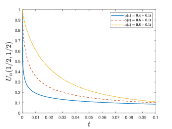
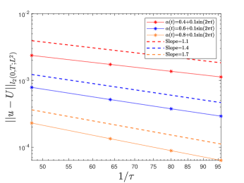
Fig. 1: (left) Plots of $U_{n}$ at $(\frac{1}{2},\frac{1}{2})$ under different $\alpha_{0}$; (right) Errors under different $\alpha_{0}$ and $\tau$.

8 An application to inverse problem

From previous results, we notice that the initial value $\alpha_{0}$ plays a critical role in determining the properties of the model. Thus, it is meaningful to determine $\alpha_{0}$ from observations of $u$, which formulates an inverse problem. Here we follow the proof of [9, Theorem 6.31] to present a preliminary result for demonstrating the usage of equivalent formulations derived by the generalized identity function.

Theorem 7.

For (1)–(2) with $f\equiv 0$, $u_{0}\in C^{\infty}_{0}$ and $\Delta u_{0}(x_{0})\neq 0$ for some $x_{0}\in\Omega$, we have

$$\alpha_{0}=\lim_{t\rightarrow 0^{+}}\frac{t\partial_{t}u(x_{0},t)}{u(x_{0},t)-u_{0}(x_{0})}.$$

Proof.

By Theorem 2 the model (1)–(2) is well-posed and could be reformulated as (10). We then further calculate the convolution of (10) with $f\equiv 0$ and $\beta_{1-\alpha_{0}}$ to get

$$\beta_{1-\alpha_{0}}*(\partial_{t}u)+\beta_{1-\alpha_{0}}*(g^{\prime}*\partial_{t}u)-\Delta u=0,$$ (71)

the solution of which could be expressed as $u=F(t)u_{0}+\mathcal{H}$ where $\mathcal{H}$ could be expressed via the Mittag-Leffler function $E_{a,b}(\cdot)$ [7]

$$\mathcal{H}:=\sum_{j=1}^{\infty}\rho*(-\beta_{1-\alpha_{0}}*(g^{\prime}*\partial_{t}u),\phi_{j})\phi_{j},~{}~{}\rho:=t^{\alpha_{0}-1}E_{\alpha_{0},\alpha_{0}}(-\lambda_{j}t^{\alpha_{0}}).$$

Also, (71) implies $\Delta u|_{\partial\Omega}=0$. Then one could follow the proof of Theorem 3 to further show that $\|\partial_{t}\Delta^{2}u\|\leq Qt^{\alpha_{0}-1}$, which will be used later.

By the derivations of [9, Theorem 6.31] we find that if we can show

$$\lim_{t\rightarrow 0^{+}}t^{1-\alpha_{0}}\partial_{t}\mathcal{H}(x_{0},t)=0\text{ and }\lim_{t\rightarrow 0^{+}}t^{-\alpha_{0}}\mathcal{H}(x_{0},t)=0,$$ (72)

then the proof of [9, Theorem 6.31] is not affected at all by the term $\mathcal{H}$ such that we immediately reach the conclusion by [9, Theorem 6.31].

To show the first statement, we first apply integration by parts to obtain

$$\mathcal{H}=\sum_{j=1}^{\infty}\frac{1}{\lambda_{j}^{2}}\rho*(-\beta_{1-\alpha_{0}}*(g^{\prime}*\partial_{t}\Delta^{2}u),\phi_{j})\phi_{j},$$

and we follow similar derivations as (23)–(26) to obtain $|\partial_{t}(\beta_{1-\alpha_{0}}*g^{\prime})|\leq t^{-\alpha_{0}-\varepsilon}$ for $0<\epsilon\ll 1-\alpha_{0}$. We invoke this and apply $\|\phi_{j}\|_{L^{\infty}}\leq Q\lambda_{j}^{\frac{\kappa}{2}}$ for $\kappa>\frac{d}{2}$ [9, Page 257] to bound $\partial_{t}\mathcal{H}$ as

$$|\partial_{t}\mathcal{H}| \leq Q\sum_{j=1}^{\infty}\frac{1}{\lambda_{j}^{2-\frac{\kappa}{2}}}\rho*\big{(}|\partial_{t}(\beta_{1-\alpha_{0}}*g^{\prime})|*\|\partial_{t}\Delta^{2}u\|\big{)}$$

$$\leq Q\sum_{j=1}^{\infty}\frac{1}{\lambda_{j}^{2-\frac{\kappa}{2}}}\rho*\big{(}t^{-\alpha_{0}-\varepsilon}*t^{\alpha_{0}-1}\big{)}\leq Q\sum_{j=1}^{\infty}\frac{1}{\lambda_{j}^{2-\frac{\kappa}{2}}}\rho*t^{-\varepsilon}.$$

We combine this with the following estimates [7]

$$\rho*t^{-\varepsilon}=\Gamma(\alpha_{0})t^{\alpha_{0}-\varepsilon}E_{\alpha_{0},1+\alpha_{0}-\varepsilon}(-\lambda_{j}t^{\alpha_{0}})\leq Q\frac{t^{\alpha_{0}-\varepsilon}}{1+\lambda_{j}t^{\alpha_{0}}}=Q\frac{t^{-\varepsilon}}{\lambda_{j}}\frac{\lambda_{j}t^{\alpha_{0}}}{1+\lambda_{j}t^{\alpha_{0}}}\leq Q\frac{t^{-\varepsilon}}{\lambda_{j}}$$

to obtain

$$t^{1-\alpha_{0}}|\partial_{t}\mathcal{H}| \leq Qt^{1-\alpha_{0}-\varepsilon}\sum_{j=1}^{\infty}\frac{1}{\lambda_{j}^{3-\frac{\kappa}{2}}}\leq Qt^{1-\alpha_{0}-\varepsilon}\sum_{j=1}^{\infty}\frac{1}{j^{\frac{2}{d}(3-\frac{\kappa}{2})}}$$

where we used the Weyl’s law $\lambda_{j}\sim j^{\frac{2}{d}}$ for $j\rightarrow\infty$. We set $\kappa=\frac{d}{2}+1$ to obtain $\frac{2}{d}(3-\frac{\kappa}{2})=\frac{5}{d}-\frac{1}{2}>1$ for $1\leq d\leq 3$. Thus we have $t^{1-\alpha_{0}}|\partial_{t}\mathcal{H}|\leq Qt^{1-\alpha_{0}-\varepsilon}$, which implies the first statement in (72). The second statement could be proved similarly and we thus omit the details. ∎

References

- [1] R. Adams and J. Fournier, Sobolev Spaces, Elsevier, San Diego, 2003.
- [2] G. Akrivis, B. Li, and C. Lubich, Combining maximal regularity and energy estimates for time discretizations of quasilinear parabolic equations. Math. Comp., 86 (2017), 1527–1552.
- [3] L. Banjai and C. Makridakis, A posteriori error analysis for approximations of time-fractional subdiffusion problems. Math. Comp. 91 (2022), 1711–1737.
- [4] E. Cuesta, M. Kirane, A. Alsaedi, B. Ahmad, On the sub-diffusion fractional initial value problem with time variable order. Adv. Nonlinear Anal. 10 (2021), 1301–1315.
- [5] L. Evans, Partial Differential Equations, Graduate Studies in Mathematics, V 19, American Mathematical Society, Rhode Island, 1998.
- [6] R. Garrappa and A. Giusti, A computational approach to exponential-type variable-order fractional differential equations. J. Sci. Comput. 96 (2023), 63.
- [7] R. Gorenflo, A. Kilbas, F. Mainardi, S. Rogosin, Mittag-Leffler Functions, Related Topics and Applications. Springer, New York, 2014.
- [8] M. Gunzburger and J. Wang, Error analysis of fully discrete finite element approximations to an optimal control problem governed by a time-fractional PDE. SIAM J. Control. Optim., 57 (2019), 241–263.
- [9] B. Jin, Fractional differential equations–an approach via fractional derivatives, Appl. Math. Sci. 206, Springer, Cham, 2021.
- [10] B. Jin, B. Li, Z. Zhou, Numerical analysis of nonlinear subdiffusion equations. SIAM J. Numer. Anal., 56 (2018), 1–23.
- [11] Y. Kian, M. Slodička, É. Soccorsi, K. Bockstal, On time-fractional partial differential equations of time-dependent piecewise constant order. arXiv:2402.03482.
- [12] Y. Kian, E. Soccorsi, M. Yamamoto, On time-fractional diffusion equations with space-dependent variable order, Ann. Henri Poincaré, 19 (2018), 3855–3881.
- [13] N. Kopteva, Error analysis of an L2-type method on graded meshes for a fractional-order parabolic problem. Math. Comp. 90 (2021), 19–40.
- [14] K. Le and M. Stynes, An -robust semidiscrete finite element method for a Fokker-Planck initial-boundary value problem with variable-order fractional time derivative. J. Sci. Comput. 86 (2021), 22.
- [15] B. Li, H. Luo, X. Xie, Analysis of a time-stepping scheme for time fractional diffusion problems with nonsmooth data, SIAM J. Numer. Anal., 57 (2019), 779–798.
- [16] D. Li, J. Zhang, Z. Zhang, Unconditionally optimal error estimates of a linearized Galerkin method for nonlinear time fractional reaction-subdiffusion equations, J. Sci. Comput. 76 (2018), 848–866.
- [17] H. Liao, T. Tang, T. Zhou, A second-order and nonuniform time-stepping maximum-principle preserving scheme for time-fractional Allen-Cahn equations. J. Comput. Phys. 414 (2020), 109473.
- [18] C. Lorenzo and T. Hartley, Variable order and distributed order fractional operators, Nonlinear Dyn., 29 (2002), 57–98.
- [19] C. Lubich, Convolution quadrature and discretized operational calculus. I and II, Numer. Math., 52 (1988) 129–145 and 413–425.
- [20] Y. Luchko, Initial-boundary-value problems for the one-dimensional time-fractional diffusion equation. Fract. Calc. Appl. Anal., 15 (2012), 141–160.
- [21] W. McLean and V. Thomée, Numerical solution of an evolution equation with a positive-type memory term. J. Austral. Math. Soc. Ser. B, 35 (1993), 23–70.
- [22] K. Mustapha and W. McLean, Discontinuous Galerkin method for an evolution equation with a memory term of positive type. Math. Comp., 78 (2009), 1975–1995.
- [23] J. Shi and M. Chen, High-order BDF convolution quadrature for subdiffusion models with a singular source term. SIAM J. Numer. Anal. 61 (2023), 2559–2579.
- [24] K. Sakamoto and M. Yamamoto, Initial value/boundary value problems for fractional diffusion-wave equations and applications to some inverse problems, J. Math. Anal. Appl., 382 (2011), 426–447.
- [25] M. Stynes, E. O’Riordan, and J. Gracia, Error analysis of a finite difference method on graded mesh for a time-fractional diffusion equation, SIAM J. Numer. Anal., 55 (2017), 1057–1079.
- [26] H. Sun, Y. Zhang, W. Chen, D. Reeves, Use of a variable-index fractional-derivative model to capture transient dispersion in heterogeneous media, J. Contam. Hydrol., 157 (2014) 47–58.
- [27] H. Sun, A. Chang, Y. Zhang, W. Chen, A review on variable-order fractional differential equations: mathematical foundations, physical models, numerical methods and applications. Fract. Calc. Appl. Anal., 22 (2019), 27–59.
- [28] V. Thomée, Galerkin Finite Element Methods for Parabolic Problems, Lecture Notes in Mathematics 1054, Springer-Verlag, New York, 1984.
- [29] S. Umarov and S.Steinberg, Variable order differential equations with piecewise constant order-function and diffusion with changing modes. Z. Anal. Anwend. 28 (2009), 131–150.
- [30] F. Zeng, Z. Zhang, G. Karniadakis, A generalized spectral collocation method with tunable accuracy for variable-order fractional differential equations, SIAM J. Sci. Comput., 37 (2015), A2710–A2732.
- [31] T. Zhao, Z. Mao, G. Karniadakis, Multi-domain spectral collocation method for variable-order nonlinear fractional differential equations. Comput. Meth. Appl. Mech. Engrg., 348 (2019), 377–395.
- [32] P. Zhuang, F. Liu, V. Anh, I. Turner, Numerical methods for the variable-order fractional advection-diffusion equation with a nonlinear source term, SIAM J. Numer. Anal., 47 (2009), 1760–1781.