Li et al.

Optimal Locally Private Linear Contextual Bandit

On the Optimal Regret of Locally Private Linear Contextual Bandit

Jiachun Li Institute for Data, Systems and Society, Massachusetts Institute of Technology, Cambridge, MA 02142, USA David Simchi-Levi Institute for Data, Systems and Society, Operations Research Center, Department of Civil and Environmental Engineering, Massachusetts Institute of Technology, Cambridge, MA 02142, USA Yining Wang Naveen Jindal School of Management, University of Texas at Dallas, Richardson, TX 75080, USA

Contextual bandit with linear reward functions is among one of the most extensively studied models in bandit and online learning research. Recently, there has been increasing interest in designing locally private linear contextual bandit algorithms, where sensitive information contained in contexts and rewards is protected against leakage to the general public. While the classical linear contextual bandit algorithm admits cumulative regret upper bounds of $\widetilde{O}(\sqrt{T})$ via multiple alternative methods, it has remained open whether such regret bounds are attainable in the presence of local privacy constraints, with the state-of-the-art result being $\widetilde{O}(T^{3/4})$. In this paper, we show that it is indeed possible to achieve an $\widetilde{O}(\sqrt{T})$ regret upper bound for locally private linear contextual bandit. Our solution relies on several new algorithmic and analytical ideas, such as the analysis of mean absolute deviation errors and layered principal component regression in order to achieve small mean absolute deviation errors.

This version:

Contextual bandit, differential privacy, principal component regression

1 Introduction

Contextual bandit with linear reward functions is among one of the most extensively studied models in bandit and online learning research. In this model, at every time period an algorithm receives a context and must select among one of the many actions. Given a pair of context and selected action, the expected reward is modeled by a $d$-dimensional linear model. The objective of the algorithm is to balance estimation of reward models and exploitation of high-reward actions, so that the cumulative reward is maximized (or equivalently, the cumulative regret is minimized). Sec. 1.1 provides a rigorous mathematical formulation of the linear contextual bandit model studied in this paper. There has been many algorithms that are designed for the linear contextual bandit problem, such as the LinUCB and SupLinUCB algorithms designed specifically for linear or generalized linear models (Abbasi-Yadkori et al. 2011, Rusmevichientong and Tsitsiklis 2010, Auer 2002, Filippi et al. 2010) and more general algorithms that apply to general function classes beyond the linear case (Auer et al. 2002, Simchi-Levi and Xu 2022, Agarwal et al. 2014, Foster and Rakhlin 2020, Xu and Zeevi 2020). While there are subtle and nuanced differences in problem settings, assumptions and regret dependency, one common feature of these existing results is that all algorithms enjoy worst-case regret upper bound at the asymptotic order of $\widetilde{O}(\sqrt{T})$ when there are $T$ time periods, which is minimax optimal for gap-free contextual bandit problems (Auer et al. 2002).

In recent years, the issue of data privacy (Dwork and Roth 2014) has received increasing interest in computer science and operations research communities, including in contextual bandit problems. This is motivated by the observation that, in many real-world applications of contextual bandit, context vectors and actions contain sensitive information such as past purchases, credit worthiness and offered prices, which should not be disclosed to the general public (Chen et al. 2023, 2022a, Fu et al. 2022, Lei et al. 2023). Using the notion of local privacy first introduced by Duchi et al. (2018), the work of Zheng et al. (2020) designed algorithms for linear and generalized linear contextual bandits with a regret upper bound of $\widetilde{O}(T^{3/4})$. While improved regret is possible with strong assumptions (especially eigenvalue-type conditions, as in (Han et al. 2021) which we also discuss in more details in Sec. 1.2), it is not known whether the regret could be improved to match $\widetilde{O}(\sqrt{T})$ in the non-private case without strong eigenvalue conditions. Indeed, it was suggested in (Zheng et al. 2020) that $\widetilde{O}(\sqrt{T})$ regret may not be possible with local privacy constraints in the general case, and lower bounds should be pursued.

In this paper, we make two contributions towards the locally private linear contextual bandit problem:

1. On the lower bound side, we formalize the intuitions behind impossibility arguments in (Zheng et al. 2020), by rigorously showing that 1) no analysis based on the mean-square error could achieve a regret upper bound lower than $\widetilde{O}(T^{3/4})$, and 2) no bandit algorithm based on input perturbation could achieve a regret upper bound lower than $\widetilde{O}(T^{2/3})$. This two (partially) negative results explain why it is so challenging to achieve $\widetilde{O}(\sqrt{T})$ regret for locally private linear contextual bandit, because many local privacy mechanisms for linear models are input perturbation methods, and virtually all existing analysis of linear or even general contextual bandit relies on the mean-square error notion.

2. On the upper bound side, we show that despite the negative results, it is actually possible to achieve $\widetilde{O}(\sqrt{T})$ regret with local privacy constraints. The algorithm and analysis that achieve this result would need to circumvent the negative results established: that they cannot be based on the analysis of the mean-square error, and they must use locally private mechanisms more sophisticated than input perturbation, which essentially rules out non-interactive local privacy mechanisms. In our analysis, we rely on the mean-absolute deviation (MAD) error and use a layered principal component regression approach to adaptively partition contextual vectors into hierarchical bins. Because of the non-standard algorithm and analysis, we believe the results of this paper would have implications to a wider class of privacy-constrained bandit problems as well. Our results also leave a sequence of follow-up works open, as we remark in the final section of this paper.

The rest of the paper is organized as follows. In the remainder of the introduction section we formally introduce the model formulation, including linear contextual bandit and locally private bandit models. We also cover some additional related works on contextual bandit and privacy and position our contributions within the literature. We then proceed to introduce two negative results and afterwards our main algorithm with regret upper bounds. Finally, we complete the paper by mentioning several interesting future research directions.

1.1 Model specification and definitions

We consider a standard linear contextual bandit model with finite number of actions and stochastic contexts. Let $\mathcal{X}$ be a compact context space and $\mathcal{A}$ be a discrete action space such that $|\mathcal{A}|\leq A<\infty$. Let $P_{\mathcal{X}}$ be an unknown distribution supported on $\mathcal{X}$. Let $\mathcal{F}$ be a hypothesis class such that each function $f\in\mathcal{F}:\mathcal{X}\times\mathcal{A}\to\mathbb{R}$ maps a pair of context and action into an expected reward. In this paper, we focus exclusively on the linear hypothesis class, for which every $f\in\mathcal{F}$ can be parameterized as

$$f(x,a)=\langle\phi(x,a),\theta_{f}\rangle,$$

where $\theta_{f}\in\mathbb{R}^{d}$, $\|\theta_{f}\|_{2}\leq 1$ is a linear model associated with the hypothesis $f\in\mathcal{F}$ and $\phi:\mathcal{X}\times\mathcal{A}\to\{z\in\mathbb{R}^{d}:\|z\|_{2}\leq 1\}$ is a known feature map that maps a context-action pair to a $d$-dimensional vector with bounded norm.

The linear contextual bandit problem consists of $T$ consecutive time periods equipped with unknown context distribution $P_{\mathcal{X}}$ and an unknown linear model $f^{*}\in\mathcal{F}$. At the beginning of time period $t\in[T]$, a context $x_{t}\sim P_{\mathcal{X}}$ is sampled from $P_{\mathcal{X}}$ and revealed to the bandit algorithm. The algorithm then must take an action $a_{t}\in\mathcal{A}$. Afterwards, a random reward $y_{t}\in[-1,1]$ is realized and observed such that

$$\mathbb{E}[y_{t}|x_{t},a_{t}]=f^{*}(x_{t},a_{t}).$$

The effectiveness of a policy $\pi$ is measured by its cumulative regret against a clairvoyant policy $\pi^{*}$ which has perfect information of $P_{\mathcal{X}}$ and $f^{*}$. More specifically, the cumulative regret of policy $\pi$ is defined as

$$\mathrm{Reg}(\pi):=\mathbb{E}^{\pi}\left[\sum_{t=1}^{T}f^{*}(x_{t},a_{t}^{*})-f_{t}(x_{t},a_{t})\right]\;\;\;\;\;\;\text{where}\;\;a_{t}^{*}=\arg\max_{a\in\mathcal{A}}f^{*}(x_{t},a).$$ (1)

It is clear from definition that $\mathrm{Reg}(\pi)$ is always non-negative, and smaller regret indicates better performance of a bandit algorithm.

A bandit algorithm or policy $\pi$ cannot make the action decision $a_{t}$ at time $t$ arbitrarily. In particular, the following two considerations are important:

1. admissibility: the policy $\pi$ with the actual context distribution $P_{\mathcal{X}}$ and model $f^{*}$ unknown, must gather data and information sequentially and make decisions only based on past data and observations;

2. privacy: the policy $\pi$, while utilizing past data and observations to learn about context distributions or the underlying reward model $f^{*}$, must respect the privacy of past data involved in such procedures, including both context vectors and realized (observed) rewards.

To formalize the two above-mentioned considerations, we use the following definition to rigorously define the class of bandit algorithms/policies allowed in this paper.

Definition 1.1

Let $\varepsilon\in(0,1]$ be a privacy parameter. A policy $\pi$ is admissible and satisfies $\varepsilon$-local differential privacy ($\varepsilon$-LDP) if and only if it can be parameterized as $\pi=(\mathfrak{A}_{1},\mathfrak{Z}_{1},\cdots,\mathfrak{A}_{T},\mathfrak{Z}_{t})$, such that for every time period $t$, the action $a_{t}\in\mathcal{A}$ and a suitably defined internal anonymized data entry $z_{t}\in\mathcal{Z}$ are generated as:

1. $a_{t}\sim\mathfrak{A}_{t}(\cdot|z_{1},\cdots,z_{t-1},x_{t})$;

2. $z_{t}\sim\mathfrak{Z}_{t}(\cdot|z_{1},\cdots,z_{t-1},x_{t},a_{t},y_{t})$;

furthermore, for every $x,x^{\prime}\in\mathcal{X}$, $a,a^{\prime}\in\mathcal{A}$, $y,y^{\prime}\in[-1,1]$, $z_{1},\cdots,z_{t-1}\in\mathcal{Z}$ and every measurable $Z\subseteq\mathcal{Z}$, it holds that

$$\frac{\mathfrak{Z}_{t}(Z|z_{1},\cdots,z_{t-1},x,a,y)}{\mathfrak{Z}_{t}(Z|z_{1},\cdots,z_{t-1},x^{\prime},a^{\prime},y^{\prime})}\leq e^{\varepsilon}.$$

Definition 1.1 is similar to the definition of adaptive local privacy in (Duchi et al. 2018), which is adapted to bandit problems in a “non-anticipating” sense standard to differentially private bandit formulations (Chen et al. 2023, 2022a, Shariff and Sheffet 2018). More specifically, when making the decision of $a_{t}$ the exact context $x_{t}$ could be utilized, and anonymization of $x_{t}$ (and $y_{t}$) only occurs after time period $t$. This is necessary because otherwise a linear regret lower bound applies, as shown in (Shariff and Sheffet 2018).

1.2 Related works

This works studies locally private linear contextual bandit, two very important questions in theoretical computer science, machine learning and operations research. For contextual bandit, some representative references include (Auer et al. 2002, Foster and Rakhlin 2020, Agarwal et al. 2014, Simchi-Levi and Xu 2022, Beygelzimer et al. 2011, Xu and Zeevi 2020). When specialized to linear or generalized linear settings, optimism is an alternative effective approach which in general could deal with adversarial contexts and potentially very large action space (Auer 2002, Rusmevichientong and Tsitsiklis 2010, Abbasi-Yadkori et al. 2011, Filippi et al. 2010). The works of Bubeck et al. (2012), Lattimore and Szepesvári (2020) provide excellent surveys on results of contextual bandit research.

The notion of differential privacy was formalized in the seminar paper of Dwork (2006) and has seen a great amount of research since then. We refer the readers to (Dwork and Roth 2014) for an excellent survey and review of progress in differential privacy research. Local differential privacy was first proposed by Duchi et al. (2018) as a strengthening to centralized differential privacy that is more applicable to learning problems and statistical analysis, and has since then become a popular differential privacy measure for a number of statistics and machine learning problems. The major difference of local differential privacy as opposed to the classical centralized privacy measure is the notion of an untrusted data aggregator, so that individual data samples must be anonymized prior to any statistical or algorithmic procedures, which is in contrast to centralized privacy that only needs to anonymize any publicized outputs. The works of (Duchi et al. 2018, Duchi and Ruan 2024) studied optimal rates of convergence for a number of models subject to local privacy constraints. Wang et al. (2023) studied sample complexity upper bounds for generalized linear model using the criterion of excess risk, which is different from model estimating errors required in the bandit setting. The work of Chen et al. (2023) also provides an overview and comparison between local and centralized privacy notions under bandit and pricing settings.

We next discuss in further details of existing works on differentially private contextual bandit research. The work of (Shariff and Sheffet 2018) is among one of the first papers studying differentially private linear bandit, by proposing the anticipating differential privacy notion and analyzing a LinUCB procedure with perturbed sufficient statistics. The paper focuses solely on the centralized privacy setting and achieves a regret upper bound of $\widetilde{O}(\sqrt{T}/\alpha)$ omitting other problem dependent parameters, where $\alpha$ is the privacy parameter. The algorithm and analysis could be easily adapted to local privacy settings achieving a regret upper bound of $\widetilde{O}(T^{3/4}/\alpha)$. Going beyond linear models, Chen et al. (2022a) extends the methods to generalized linear pricing models under centralized privacy settings, requiring more sophisticated methods such as perturbed MLE and tree-based covariance anonymizations. Lei et al. (2023) studies a similar model under offline settings and both centralized and local privacy notions. Chen et al. (2023) studies local privacy algorithms for non-parametric contextual pricing models, built upon the models introduced by Chen and Gallego (2021). The works of Zheng et al. (2020), Han et al. (2021) studied local privacy algorithms for generalized linear models.

The work of Han et al. (2021) achieves $\widetilde{O}(\sqrt{T}/\alpha)$ regret for locally private generalized linear bandit, under the additional assumption that the context vectors are relatively “spread-out” so that the least eigenvalue of the sample covariance or the projection of the context vectors is not too small. Such eigenvalue type conditions potentially make the problem much easier. For example, for purely linear models if the sample covariance $\Lambda$ after $n$ time periods satisfies $\Lambda\succeq\Omega(1)\cdot I$, then it is not difficult to prove that the anonymized sample covariance $\widehat{\Lambda}$ satisfies spectral approximation $\widehat{\Lambda}-\Lambda\preceq\widetilde{O}_{P}(1/\sqrt{n})\cdot\Lambda$ with high probability, which then translates to an $\widetilde{O}(\sqrt{T}/\alpha)$ regret. When $\Lambda$ is not well-conditioned (e.g. $\lambda_{\min}(\Lambda)$ growing significantly slower than $O(n)$ while $\lambda_{\max}(\Lambda)$ grows linearly as $\Omega(n)$), however, such spectral approximation may not hold and the best one can obtain from such a procedure is an $\widetilde{O}(T^{3/4}/\alpha)$ regret. For generalized linear models, while algorithms are different (as we no longer have simple sufficient statistics), similar phenomenon is also observed by Chen et al. (2022a) which shows that with additional eigenvalue conditions the regret of a centralized private algorithm could be vastly improved.

A closely related bandit question to what we studied is the so-called linear bandit, for each time period a bandit algorithm selects an action $a_{t}$ from a fixed action space $\mathcal{A}$ each time without observing contexts and the rewards given action $a_{t}\in\mathcal{A}$ is modeled by a linear function. While similar in appearance, such settings are fundamentally different from linear contextual bandit because there is no context and therefore actions are usually not considered sensitive since they are selected solely by the algorithm. Hanna et al. (2022) studied local and central differential privacy under this setting and obtain near-optimal regret using variations to experimental design type algorithms. The work of Hanna et al. (2023) shows that linear contextual bandit can be reduced to a sequence of linear bandit problems without contexts. However, such reduction uses all historical data and is less likely to be amenable to local privacy constraints.

2 Motivating negative results and examples

Before presenting our algorithm and analysis, we discuss several motivating negative examples and results which shed light on why the locally private contextual bandit problem is technically challenging. For simplicity, in this section all problem setups are offline: they are sufficient to demonstrate that certain important steps in existing contextual bandit analysis cannot be adapted under local privacy settings, or popular local private estimation techniques cannot be directly applied to deliver tight bounds for contextual bandit problems.

2.1 Fundamental limits of the mean-square error

Most existing works on (linear) contextual bandit rely on estimating the underlying model with small mean-square errors. More specifically, let $\mathcal{D}$ be an unknown distribution supported on a compact subset of $\mathbb{R}^{d}$ and $\phi_{1},\cdots,\phi_{n}\overset{i.i.d.}{\sim}\mathcal{D}$. Let $y_{1},\cdots,y_{n}\in\mathbb{R}$ be noisy labels such that $\mathbb{E}[y_{i}|\phi_{i}]=\phi_{i}^{\top}\theta^{*}$. It is possible to obtain an estimate $\widehat{\theta}_{n}$ based on $\{(x_{i},y_{i})\}_{i=1}^{n}$ such that with high probability,

$$\mathbb{E}_{\phi\sim\mathcal{D}}\left[\big{|}\phi^{\top}(\widehat{\theta}_{n}-\theta^{*})\big{|}^{2}\right]=(\widehat{\theta}_{n}-\theta^{*})^{\top}\Lambda_{\mathcal{D}}(\widehat{\theta}_{n}-\theta^{*})=\widetilde{O}(n^{-1}),$$ (2)

where $\Lambda_{\mathcal{D}}=\mathbb{E}_{\mathcal{D}}[\phi\phi^{\top}]$ and in the $\widetilde{O}(\cdot)$ notation we omit polynomial dependency on $d$ and $\ln n$. Without privacy considerations, Eq. (2) could be attained by simply using the ordinary least-squares, or its penalized version. The work of Simchi-Levi and Xu (2022) (Bypassing-the-Monster) and Foster et al. (2018) (RegCB) specifically rely on such oracles with $\widetilde{O}(n^{-1})$ convergence rate in order to obtain an $\widetilde{O}(\sqrt{T})$ cumulative regret. For the more classical LinUCB (Abbasi-Yadkori et al. 2011, Rusmevichientong and Tsitsiklis 2010), SupLinUCB (Auer 2002) or high-dimensional regression algorithms (Chen et al. 2022b, Bastani and Bayati 2020) designed specifically for linear models, the guarantee of Eq. (2) is also essential in the regret analysis. All of these existing works on (linear) contextual bandit share the following two important properties:

1. Eq. (2) must be established for any distribution $\mathcal{D}$ supported on (a compact subset of) $\mathbb{R}^{d}$, because the policy assignments of actions will alter the distributions of $\phi$ which are essentially out of control of the bandit algorithm;

2. The right-hand side of Eq. (2) must be on the order of $\widetilde{O}(n^{-1})$, so that after certain Cauchy-Schwarz relaxations the resulting cumulative regret is upper bounded by $\widetilde{O}(\sqrt{T})$, omitting polynomial dependency on $d$ and $\ln T$ terms.

In the following result, we show, quite surprisingly, that Eq. (2) is impossible for any locally private estimators on general $\mathcal{D}$ distributions.

Theorem 2.1

Fix $\alpha\in(0,1]$ and $d=2$. There exists a numerical constant $\underline{C}_{1}>0$ such that the following holds: for any $n\geq 1$, there exists a distribution $\mathcal{D}_{n}$ supported on $\{x\in\mathbb{R}^{d}:\|x\|_{2}\leq 1\}$ and parameter class $\Theta_{n}\subseteq\{\theta\in\mathbb{R}^{d}:\|\theta\|_{2}\leq 1\}$ such that for any estimate $\widehat{\theta}_{n}$ that is $\alpha$-locally private,

$$\sup_{\theta^{*}\in\Theta_{n}}\mathbb{E}_{\theta^{*},\mathcal{D}_{n}}\left[(\widehat{\theta}_{n}-\theta^{*})^{\top}\Lambda_{\mathcal{D}_{n}}(\widehat{\theta}_{n}-\theta^{*})\right]\geq\frac{\underline{C}_{1}}{(e^{\alpha}-1)\sqrt{n}},$$

where $\Lambda_{\mathcal{D}_{n}}=\mathbb{E}_{\mathcal{D}_{n}}[\phi\phi^{\top}]$.

Theorem 2.1 is proved using the information-theoretical tools developed in (Duchi et al. 2018) and is given in the supplementary material. Its basic idea is simple: we design the distribution $\mathcal{D}$ in such a way that one particular direction is explored with only probability $1/\sqrt{n}$. More specifically,

$$\phi\sim\mathcal{D}_{n}:\;\;\;\;\;\;\phi=\left\{\begin{array}[]{ll}e_{1}&\text{ with probability $1-1/\sqrt{n}$},\\ e_{2}&\text{ with probability $1/\sqrt{n}$}.\end{array}\right.$$ (3)

With local privacy constraints, it can be proved rigorously that no procedure can detect such exploration with high probability (think about counting the occurrences of a particular event: if the event only occurs $O(\sqrt{n})$ times out of $n$ total periods then no locally private method can recover the count accurately). On the other hand, because the direction is explored with probability at least $1/\sqrt{n}$, failure to estimate along the direction leads to an MSE of at least $\Omega(1/\sqrt{n})$, completing the proof.

Theorem 2.1 shows that for general distribution $\mathcal{D}$, no locally private procedure could attain a mean-square error at the rate of $\widetilde{O}(1/n)$. Instead, the best one can do is $\widetilde{O}(1/\sqrt{n})$ for the mean-square error. This combined with Cauchy-Schwarz inequalities in existing analysis (e.g. Bypassing the monster (Simchi-Levi and Xu 2022) or LinUCB (Abbasi-Yadkori et al. 2011, Rusmevichientong and Tsitsiklis 2010)) leads to a regret of $\widetilde{O}(T^{3/4})$, which is sub-optimal. Coincidentally, the regret scaling of $\widetilde{O}(T^{3/4})$ is the same with bounds obtained in (Zheng et al. 2020), which is unsurprising in light of Theorem 2.1 because the approach and analysis in (Zheng et al. 2020) are founded on mean-square errors, which must suffer from such fundamental limitations.

2.2 Fundamental limits of input perturbation

It is tempting to consider the result in Theorem 2.1 as an artifact of the mean-square error because the lower bound is constructed for a particular type of distribution that explores some directions with very small probability. For such distributions, one might conjecture that the mean-absolute deviation

$$\mathbb{E}_{\phi\sim\mathcal{D}}\left[\big{|}\phi^{\top}(\widehat{\theta}_{n}-\theta^{*})\big{|}\right]$$

is a more proper error measure. By Jensen’s inequality if the MSE is $\widetilde{O}(1/n)$ then the above error measure is upper bounded by $\widetilde{O}(1/\sqrt{n})$ but the inverse is not true: in the constructed counter-examples in Theorem 2.1 both error measures evaluate to $\widetilde{O}(1/\sqrt{n})$. It might be the case that we may still use existing contextual bandit algorithms with simple local privacy procedures such as input perturbation, only changing the analysis that circumvents the MSE in a smart way and analyzing the mean absolute deviation instead.

Our following theorem shows that this is not the case. In particular, if one uses input perturbation to satisfy local privacy constraints, then no estimator could perform well even with the mean absolute deviation measure.

Theorem 2.2

Fix $\alpha\in(0,1]$ and $d=2$. There exists a numerical constant $\underline{C}_{2}>0$ such that the following holds: for any $n\geq 1$, there exists a distribution $\mathcal{D}_{n}$ supported on $\{x\in\mathbb{R}^{d}:\|x\|_{2}\leq 1\}$ and parameter class $\Theta_{n}\subseteq\{x\in\mathbb{R}^{d}:\|x\|_{2}\leq 1\}$ such that for any estimator $\widehat{\theta}_{n}$ obtained with input $\{\widetilde{\phi}_{i},\widetilde{y}_{i}\}_{i=1}^{n}$, where $\widetilde{\phi}_{i}=\phi_{i}+\mathrm{Lap}_{d}(0,\alpha^{-1})$, $\widetilde{y}_{i}=y_{i}+\mathrm{Lap}_{1}(0,\alpha^{-1})$, $\phi_{i}\overset{i.i.d.}{\sim}\mathcal{D}_{n}$, $y_{i}=\phi_{i}^{\top}\theta^{*}$ and $\mathrm{Lap}_{d}(\mu,\sigma)$ is the distribution of a $d$-dimensional vector with i.i.d. components that are distributed as a Laplace distribution with mean $\mu$ and scale parameter $\sigma$,

$$\sup_{\theta^{*}\in\Theta_{n}}\mathbb{E}_{\mathcal{D}_{n},\theta^{*}}\left[\mathcal{E}_{\mathrm{MAD}}(\widehat{\theta}_{n},\theta^{*};\mathcal{D}_{n})\right]\geq\frac{\underline{C}_{2}}{\sqrt[3]{n}},$$

where $\mathcal{E}_{\mathrm{MAD}}(\widehat{\theta},\theta^{*};\mathcal{D})=\mathbb{E}_{\phi\sim\mathcal{D}}[|\phi^{\top}(\widehat{\theta}-\theta^{*})|]$ is the mean absolute deviation error of $\widehat{\theta}$ with respect to $\mathcal{D}$.

Before commenting how Theorem 2.2 is proved, we first comment on its implications. In the setup of this theorem there is a noiseless linear regression problem $y_{i}=\phi_{i}^{\top}\theta^{*}$ but both the feature vectors $\{\phi_{i}\}_{i=1}^{n}$ and the labels $\{y_{i}\}_{i=1}^{n}$ are anonymized using Laplace mechanism into $\{\widetilde{\phi}_{i},\widetilde{y}_{i}\}_{i=1}^{n}$, a technique known as input perturbation in differential privacy research (Dwork and Roth 2014). Afterwards any estimator based on $\{\widetilde{\phi}_{i},\widetilde{y}_{i}\}_{i=1}^{n}$ is automatically differentially private due to closeness to post-processing. Theorem 2.2 essentially shows that such a straightforward approach of input perturbation cannot succeed, by demonstrating that any estimator based on the anonymized inputs $\{\widetilde{\phi}_{i},\widetilde{y}_{i}\}_{i=1}^{n}$ must have a mean absolute deviation error of $\Omega(n^{-1/3})$, falling short of the desired $\widetilde{O}(n^{-1/2})$ rate. As a result, more sophisticated local privacy methods beyond input perturbation must be designed to succeed.

We remark that many existing approaches to locally private contextual bandit are based on or could be easily re-formulated as input perturbation. For example, for purely linear models a common approach is to maintain the sufficient statistics $\Lambda=\sum_{i=1}^{n}\phi_{i}\phi_{i}^{\top}$ and $\mu=\sum_{i=1}^{n}y_{i}\phi_{i}$, which can be done using Wishart and Laplace mechanisms. Such an approach is not sufficient to obtain $\sqrt{T}$-regret results, as implied by Theorem 2.2.

The complete proof of Theorem 2.2 is given in the supplementary material. At a high level, the proof is based on the following idea: the design distribution $\mathcal{D}_{n}$ is constructed in the following manner:

$$\phi\sim\mathcal{D}_{n}:\;\;\;\;\;\;\phi=\left\{\begin{array}[]{ll}(1/2,n^{-1/3})&\text{ with probability $1/2$},\\ (1/2,-n^{-1/3})&\text{ with probability $1/2$}.\end{array}\right.$$

Then the distribution of the second component of the anonymized $\widetilde{\phi}$ is a mixture of Laplace distributions with symmetric means. Because such mixture distribution is exactly degenerate, there is no statistical methods that could actually estimate the mixture means, similar to the phenomenon observed in (Chen 1995) for Gaussian mixture models and the more recent works of Ho and Nguyen (2019, 2016) for more general finite mixture models. The actual proof is based on the analysis of $\chi^{2}$-divergence between degenerate mixture models with different number of mixtures, which explicitly demonstrates the singularity exhibited in the mixture distributions.

2.3 Discussion: necessity of input partitioning

We further deepen the discussion of how to obtain $\widetilde{O}(\sqrt{T})$ regret for locally private linear contextual bandit, in light of the above negative examples. Let $\delta\asymp 1/\sqrt{n}$ be a small positive number and consider the following two scenarios for $d=2$:

$$\text{Case I}:\;\;\phi=\left\{\begin{array}[]{ll}e_{1},\text{ with prob.~{}$1-\delta$},\\ e_{2},\text{ with prob.~{}$\delta$};\end{array}\right.\quad\text{ vs. }\quad\text{Case II}:\;\;\phi=\left\{\begin{array}[]{ll}(1,\sqrt{\delta}),\text{ with prob.~{}$0.5$},\\ (1,-\sqrt{\delta}),\text{ with prob.~{}$0.5$}.\end{array}\right.$$ (8)

The two scenarios are similar to the two adversarial examples for Theorems 2.1 and 2.2, respectively, and have almost the same covariance matrix of $\mathrm{diag}(1,\delta)$. However, a locally private algorithm must treat these two scenarios very differently:

1. In case I, it is not necessary and indeed not possible to do anything on the second direction, because that direction only appears for $O(\sqrt{n})$ times out of $n$ time periods which cannot be detected with local privacy constraints;

2. In case II, it is mandatory that the algorithm estimate the linear model along the second direction, because otherwise the regret could be $O(n^{3/4})$. Such estimation cannot be done using simple input perturbation, as demonstrated by Theorem 2.2. However, if we know that only small entries would appear on the second direction, we could elect to privatize $(\phi_{1},\phi_{2}/\sqrt{\delta})$ which still has constant sensitivity levels, thereby significantly reducing the variance along the second direction.

The above observations motivate us to consider “input partitioning” strategies, which partitions the input vectors into several different bins and calibrate heteroskedastic noises into them. This also helps eliminate infrequent regions that cannot be estimated (so that they will not interfere with model estimations at other regions). This principle of partitioning of input vectors will be carried out through out our algorithm design in the remainder of this paper.

3 Action elimination framework

To give a high-level description of our proposed policy and also isolate the particularly challenging part of locally private linear contextual bandit, we first describe and analyze an active elimination framework that assumes the access to a locally private offline regression oracle with uniform confidence intervals. The algorithm and analysis in this section are relatively simple and inspired heavily by the RegCB.Elimination algorithm in (Foster et al. 2018), with two important differences. First, in our setting point-wise confidence intervals could be constructed in a uniform manner, which greatly simplifies the algorithm and attains optimal regret bounds. Second, in our setting only the mean absolute deviation (MAD) error could be used, as discussed in the previous section. As a result, certain steps of the analysis needs to be revised.

3.1 Locally private offline regression oracle with confidence intervals

In this section we describe the definition of a locally private online regression oracle with confidence intervals, which is then used in Algorithm 1 to construct a contextual bandit algorithm. For notational simplicity, we augment $\mathcal{X}$ to include a “dummy” context $\perp\in\mathcal{X}$ such that $f^{*}(\perp,a)=0$ for all $a\in\mathcal{A}$. Let $\alpha,\delta\in(0,1]$ be the privacy parameter and the failure probability.

Definition 3.1 (Locally private offline oracle with confidence intervals)

A sequence of offline oracles $\{\mathcal{O}_{n}\}_{n\in\mathbb{N}}$ is equipped with error measures $\{\mathcal{E}_{\alpha,\delta}(n)\}\subseteq\mathbb{R}_{+}$ with privacy parameter $\alpha\in(0,1]$ and failure probability $\delta\in(0,1]$, if each $\mathcal{O}_{n}$ could be parameterized as $\mathcal{O}_{n}=(\mathfrak{Z}_{1},\cdots,\mathfrak{Z}_{n},\mathfrak{O})$ such that for every $i\in[n]$, an internal entry $z_{i}\in\mathcal{Z}$ is obtained with $z_{i}\sim\mathfrak{Z}_{i}(\cdot|z_{1},\cdots,z_{i-1},x_{i},a_{i},y_{i})$, and after $n$ time periods an estimate $\widehat{f}:\mathcal{X}\times\mathcal{A}\to[-1,1]$ and confidence interval $\Delta:\mathcal{X}\times\mathcal{A}\to[-1,1]$ are obtained by $\widehat{f},\Delta=\mathfrak{O}(z_{1},\cdots,z_{n})$, such that the following hold:

1. (Privacy). For every $i\in[n]$, $z_{1},\cdots,z_{i-1}\in\mathcal{Z}$, $x,x^{\prime}\in\mathcal{X}$, $a,a^{\prime}\in\mathcal{A}$, $y,y^{\prime}\in[-1,1]$ and measurable $Z\subseteq\mathcal{Z}$, $\mathfrak{Z}_{i}(Z|z_{1},\cdots,z_{i-1},x,a,y)\leq e^{\alpha}\mathfrak{Z}_{i}(Z|z_{1},\cdots,z_{i-1},x^{\prime},a^{\prime},y^{\prime})$;

2. (Utility). For every distribution $\mathcal{D}$ supported on $\mathcal{X}\times\mathcal{A}$, let $(x_{1},a_{1}),\cdots,(x_{n},y_{n})\overset{i.i.d.}{\sim}\mathcal{D}$, and $y_{1},\cdots,y_{n}$ realized according to Eq. (1). With probability $1-\delta$, the following hold:

   1. For every $x,a\in\mathcal{X}\times\mathcal{A}$, $|\widehat{f}(x,a)-f^{*}(x,a)|\leq\Delta(x,a)$;

   2. $\mathbb{E}_{(x,a)\sim\mathcal{D}}[\Delta(x,a)]\leq\mathcal{E}_{\alpha,\delta}(n)$;

   3. $\Delta(\perp,a)=0$ for all $a\in\mathcal{A}$.

Intuitively, Definition 3.1 defines an oracle that estimates a contextual reward function $f$ from offline data in a locally private fashion. In addition, the oracle also returns a point-wise confidence interval $\Delta(\cdot,\cdot)$ that is valid with high probability uniformly over all action-state pairs. Using the confidence intervals, the mean-absolute deviation error of the learning procedure is also upper bounded by $\mathcal{E}_{\alpha,\delta}(n)$ with high probability, corresponding to the second property in the utility guarantees of Definition 3.1.

3.2 The action elimination algorithm

Algorithm 1 The action elimination (RegCB.Elimination) algorithm, simplified

1:Input: time horizon $T$, oracles $\{\mathcal{O}_{n}\}_{n\in\mathbb{N}}$ with privacy parameter $\alpha$ and failure probability $\delta=1/T^{2}$, epoch schedule $n_{1},n_{2},\cdots$.

2:Initialize: $\widehat{f}_{1}^{a}(\cdot)\equiv 0$ and $\Delta_{1}^{a}(\cdot)\equiv 1$ for all $a\in\mathcal{A}$.

3:for $\tau=1,2,\cdots$ until $T$ time periods have elapsed do

4:     Initialize $A$ oracles $\{\mathcal{O}_{n}^{a}\}_{a\in\mathcal{A}}$ with $n=n_{\tau}$;

5:     for the next $n_{\tau}$ time periods do

6:         Observe $x_{t}\sim P_{\mathcal{X}}$ and initialize $\mathcal{A}_{0}(x_{t})\leftarrow\mathcal{A}$;

7:         for $\tau^{\prime}=1,2,\cdots,\tau$ do

8:              $\mathcal{A}_{\tau^{\prime}}(x_{t})\leftarrow\{a\in\mathcal{A}_{\tau^{\prime}-1}:\widehat{f}_{\tau^{\prime}}^{a}(x_{t})+\Delta_{\tau^{\prime}}^{a}(x_{t})\geq\max_{a^{\prime}\in\mathcal{A}_{\tau^{\prime}-1}}\widehat{f}_{\tau^{\prime}}^{a^{\prime}}(x_{t})-\Delta_{\tau^{\prime}}^{a^{\prime}}(x_{t})\}$;

9:         end for

10:         Take action $a_{t}\sim\mathrm{Uniform}(\mathcal{A}_{\tau}(x_{t}))$ and observe realized reward $y_{t}$;

11:         Feed $(x_{t},a_{t},y_{t})$ into $\mathcal{O}_{n}^{a_{t}}$ and $(\perp,a,0)$ into $\mathcal{O}_{n}^{a}$ for all $a\neq a_{t}$;

12:     end for

13:     For every $a\in\mathcal{A}$, obtain $\widehat{f}_{\tau+1}^{a}(\cdot)=\widehat{f}(\cdot,a)$ and $\Delta_{\tau+1}^{a}(\cdot)=\Delta(\cdot,a)$ from $\mathcal{O}_{n}^{a}$.

14:end for

In this section, assuming the availability of an oracle defined in the previous section, we describe the RegCB.Elimination algorithm in (Foster et al. 2018) and show how an upper bound on its regret could be established. Algorithm 1 describes the pseudocode of a simplified version of the RegCB.Elimination algorithm. The main difference and simplification comes from the availability of an explicitly constructed point-wise confidence interval $\Delta(\cdot,\cdot)$ from the input oracle. In contrast, the work of Foster et al. (2018) assumes no such confidence interval and therefore must resort to more complex procedures to carry out context-specific successive elimination of actions.

The following theorem upper bounds the cumulative regret of Algorithm 1, using MAD error bounds $\{\mathcal{E}_{\alpha,\varepsilon}(\cdot)\}$ in the definition of the oracles $\{\mathcal{O}_{n}\}$. The theorem is stated in generality without specifying how epoch lengths $n_{1},n_{2},\cdots$ are set. The epoch schedules will be specified later when after we describe and analyze the regression oracles to arrive at a final regret bound.

Theorem 3.2

The policy presented in Algorithm 1 satisfies $\alpha$-local differential privacy as defined in Definition 1.1. Furthermore, jointly with the success conditions in Definition 3.1 for all $\mathcal{O}_{n}^{a}$ and all epochs $\tau$, the cumulative regret of Algorithm 1 is upper bounded by

$$O\left(n_{1}+A^{2}\sum_{\tau=2}^{\tau_{0}}n_{\tau}\mathcal{E}_{\alpha,\delta}(n_{\tau-1})\right),$$

where $\tau_{0}$ is the last epoch in the execution of the algorithm.

Theorem 3.2 can be proved following roughly the same analysis in (Foster et al. 2018), with only minor modifications. For completeness, we place a complete rigorous proof of Theorem 3.2 in the supplementary material. The high-level idea is to show that (with high probability) the action sets $\mathcal{A}(x)$ always contain the optimal action $a^{*}(x)=\arg\max_{a\in\mathcal{A}}f(x,a)$, and that because uniform sampling over active actions is employed, an action that has not been eliminated receives at least $1/A$ of exploration probability from previous epochs.

Before proceeding, we remark that Theorem 3.2 only applies to bandit problems with stochastic contexts and a finite number of actions. Neither the stochasticity nor the polynomial dependency on action space size $A$ could be removed using this algorithm, because the assumed regression oracle only operate on offline data and the minimum exploration probability scales inverse polynomially with $A$. In Sec. 5 we further discuss this aspect and potential ways to remove stochasticity or finiteness assumptions.

4 Layered private linear regression (LPLR)

The purpose of this section is to design a locally private offline regression oracle with confidence intervals so that it provably satisfy the properties listed in Definition 3.1. As shown by Sec. 2, this is not an easy task and cannot be accomplished by simple approaches such as input perturbation, or vanilla ordinary least squares.

Throughout this section we assume $\phi_{1},\phi_{2},\cdots\overset{i.i.d.}{\sim}\mathcal{D}$ where $\mathcal{D}$ is an unknown distribution supported on $\mathcal{X}_{\phi}=\{\phi\in\mathbb{R}^{d}:\|\phi\|_{2}\leq 1\}$. It is induced by the distribution of $\phi_{i}=\phi(x_{i},a_{i})$ where the context-action pairs $\{(x_{i},a_{i})\}$ are i.i.d. Given $\phi_{i}\in\mathcal{X}_{\phi}$, the realized reward $y_{i}$ satisfies $\mathbb{E}[y_{i}|\phi_{i}]=\phi_{i}^{\top}\theta^{*}$. We also assume for convenience that there are $2nd$ samples available because our method operations iteratively with $d$ iterations. Finally, if an oracle received the empty context $x_{i}=\perp$, we will send to the oracle $\phi_{i}=(0,\cdots,0)$ and $y_{i}=0$.

4.1 Key idea: Adaptive layered partitioning of $d$-dimensional space

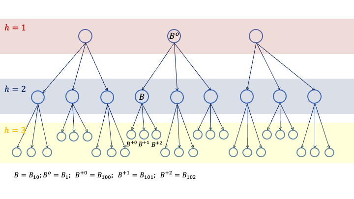
Figure 1: Illustration of an example layered partitioning of $3$-dimensional space

Note: $M=3$, while the inactive bins (with maximum $k_{h}$ being equal to 3) are neglected. For a particular bin $B=B_{10}$ on the second layer with $k_{1}=1$, $k_{2}=0$, bin $B^{o}$ is its unique parent bin on the first layer and $B^{+0}$, $B^{+1}$, $B^{+2}$ are three child bins on the immediate next layer (layer 3).

We first introduce the core concept of our method that involves a layered/hierarchical partition of $\mathcal{X}_{\phi}$ into small bins. The partition is constructed adaptively over $d$ iterations, each iteration expanding the hierarchical partition with one more layer based on the distribution $\mathcal{D}$ of input covariates. We also introduce notations for such layered partitioning that will be useful later when describing and analyzing our proposed algorithm.

Let $\beta>0$ be a small, positive parameter and denote $\gamma=T^{\beta}$, $M=\lceil 1/(2\beta)\rceil$. The hierarchical partitioning tree has $d$ layers in total, illustrated in Figure 1. We call a bin $B=B_{k_{1}\cdots k_{h}}$ a partitioning bin if $k_{1},\cdots,k_{h}<M$, because these are the bins that will be partitioned at further layers The first layer has $M$ partitioning bins. For each partitioning bin on layer $h$, $h<d$, it is further partitioned into $M$ partitioning bins on layer $h+1$. Therefore, layer $h$ would have a total of $M^{h}$ partitioning bins. Such structure also means that we can uniquely identify any bin $B$ on layer $h$ with $B=B_{\boldsymbol{k}}$ where $\boldsymbol{k}=(k_{1},\cdots,k_{h})\in\{0,1,\cdots,M\}^{h}$. This means that the parent bins of $B$ on layer $h-1$ is $B_{k_{1}\cdots k_{h-1}}$, on layer $h-2$ is $B_{k_{1}\cdots k_{h-2}}$, etc., and on the first layer is $B_{k_{1}}$. To further simplify notations regarding parents (on previous/higher layers) and children (on later/lower layers) bins as follows. Given a bin $B=B_{\boldsymbol{k}}$, $\boldsymbol{k}=(k_{1},\cdots,k_{h})$ on the $h$-th layer, define the following:

1. $B^{o}=B_{k_{1}\cdots k_{h-1}}$ is the immediate parent bin of $B$ on the $(h-1)$th layer. $B^{-2}=(B^{o})^{o}$ is the parent bin of $B^{o}$, $B^{-3}=(B^{-2})^{o}$ is the parent bin of $B^{-2}$, etc;

2. For $\ell_{1},\ell_{2},\cdots\in\{0,1,\cdots,M\}$, $B^{+\ell_{1}}=B_{k_{1}\cdots k_{h}\ell_{1}}$ is a child bin of $B$ on level $h+1$, $B^{+\ell_{1}\ell_{2}}=B_{k_{1}\cdots k_{h}\ell_{1}\ell_{2}}$ is a child bin of $B^{+\ell_{1}}$ on level $h+2$, etc.

For each bin $B$ on the $h$th layer, we maintain the following statistics. These statistics or quantities are updated in a manner that will satisfy $\alpha$-local differential privacy as defined in property 1 of Definition 3.1.

1. $\widehat{c}_{B}\in\mathbb{R}$ and $\widehat{\psi}_{B}=\widehat{c}_{B}/n$, estimation of frequency and relative frequency of bin $B$;

2. $\widehat{\Lambda}_{B}\in\mathbb{R}^{d\times d}$ and $\widehat{\lambda}_{B}\in\mathbb{R}^{d}$, estimates of the conditional covariance and vector in bin $B$;

3. $\widehat{u}_{B}\in\mathbb{R}^{d}$ a vector of unit $\ell_{2}$ norm and $\widehat{s}_{B}\in\mathbb{R}_{+}$. Furthermore, it is guaranteed that $\widehat{u}_{B}$ is orthogonal to $\widehat{u}_{B^{o}}$, $\widehat{u}_{B^{-2}}$, etc. These quantities characterize the eigenspace partitioning; furthermore, $\widehat{u}_{b},\widehat{s}_{b}$ are set to zero for non-partitioning bins or inactive bins, which will be specified later in the algorithm;

4. $\widehat{\theta}_{B}\in\mathbb{R}^{d}$, an estimated model at bin $B$ obtained via (locally private) principal component regression. It is also guaranteed that $\widehat{\theta}_{B}$ is on the same direction of $\widehat{u}_{B}$, or more specifically $\widehat{\theta}_{B}=\widehat{u}_{B}\widehat{u}_{B}^{\top}\widehat{\theta}_{B}$;

5. $\widehat{\eta}_{B},\widehat{\chi}_{B}:\mathcal{X}_{\phi}\to[0,1]$ and $\widehat{\varepsilon}_{B}\in\mathbb{R}$: upper bounds on partial predictive errors.

For each vector $\phi\in\mathcal{X}_{\phi}$ associated with $y\in[-1,1]$, there exists a unique bin at each level $h$ to which $\phi$ belongs, and for such bin a revised vector $\phi_{h}\in\mathcal{X}_{\phi}$ and a revised reward $y_{h}\in[-1,1]$ are associated with. They are determined by the following iterative procedure:

$\phi_{1}=\phi$, $y_{1}=y$; For $h=1,2,3,\cdots,d$ do: $k_{h}=\max\{k\leq M:\|\phi_{h}\|_{2}\leq\gamma^{-k}\}$ and $\phi$ belongs to $B(h)=B_{k_{1}\cdots k_{h}}$ on level $h$; $\phi_{h+1}=(I-\widehat{u}_{B(h)}\widehat{u}_{B(h)}^{\top})\phi_{h}$ and $y_{h+1}=y_{h}-\langle\phi_{h},\widehat{\theta}_{B(h)}\rangle$.

Figure 2: Iterative procedure of partitioning $(\phi,y)$

We write $k_{h}(\phi)$ for the unique integer between $0$ and $M$ determined by the above procedure at layer $h$, and $\boldsymbol{k}(\phi)=(k_{1}(\phi),\cdots,k_{d}(\phi))$. Sometimes we also write $\phi\in B$ if $\phi$ belongs to bin $B$ and $\phi\notin B$ otherwise.

4.2 Overview of the algorithm

Algorithm 2 The LPLR algorithm with $nd$ samples

1:for $h=1,2,\cdots,d$ do

2:     Initialize all bins on level $h$ so that all quantities are zero;

3:     for $i=1,2,\cdots,n$ do

4:         Observe $\phi_{i}$, $y_{i}$ and let $B_{k_{1}\cdots k_{h}}$ be the bin on level $h$ determined by Figure 2;

5:         $\textsc{LPLR-Update}(B,\phi_{i},y_{i},\alpha)$ for $B=B_{k_{1}\cdots k_{h}}$;

6:         $\textsc{LPLR-Update}(B,\perp,\perp,\alpha)$ for all $B\neq B_{k_{1}\cdots k_{h}}$ on level $h$;

7:     end for

8:     For every $B$ on level $h$, $\widehat{u}_{B},\widehat{s}_{B},\widehat{\theta}_{B}\leftarrow\textsc{LPLR-PCR}(B,n)$;

9:     With $n$ additional samples $\{(\phi_{i},y_{i})\}_{i=1}^{n}$, $\{\widehat{\eta}_{B},\widehat{\chi}_{B}\}\leftarrow\textsc{LPLR-CI}(h,\{(\phi_{i},y_{i})\}_{i=1}^{n},\alpha)$;

10:end for

11:$\widehat{f}(\cdot),\widehat{\Delta}(\cdot)\leftarrow\textsc{LPLR-Aggregate}(\{B\},n)$.

Algorithm 2 gives a pseudocode description of the algorithm that we use to construct the oracle defined in Sec. 3.1. It involves several sub-routines which will be explained in much more details later. At a higher level, Algorithm 2 uses $2n$ i.i.d. samples and partitions them into $d$ groups. For each dimension $i\in[d]$, the algorithm first uses a sample of size $n$ to update cumulative statistics of all bins on layer $i$ in a locally private fashion, via calls to the LPLR-Update sub-routine. Afterwards, for each bin on layer $i$ that has received a sufficient number of samples, a (noisy) principal component regression estimator is fit using the anonymized cumulative statistics, via calls to the LPLR-PCR sub-routine. As a last step, a fresh set of $n$ samples is used to estimate and construct point-wise confidence intervals via the LPLR-CI sub-routine. After all $d$ iterations and the tree is expanded to a full $d$ layers, the LPLR-Aggregate sub-routine aggregates all principal component regressors and confidence intervals on all layers to arrive at a final model estimate and confidence interval.

4.3 The LPLR-Update subroutine.

Algorithm 3 gives a pseudocode description of the LPLR-Update sub-routine. It updates the important cumulative statistics $\widehat{c}_{B}$, $\widehat{\Lambda}_{B}$ and $\widehat{\lambda}_{B}$ for each bin $B$ on a particular layer in the partition tree. The update procedure calibrates Laplace or Wishart noises so that it is locally private. Importantly, the magnitudes of calibrated noises are heterogeneous across the different partitioned bins, which is essential to our later analysis.

The distributions of the calibrated noise variables are rigorous defined as follows. Given $m\in\mathbb{N}$ and $\mu\in\mathbb{R}$, $b>0$, a random vector $u\in\mathbb{R}^{m}$ is drawn from the vector Laplace distribution $v\sim\mathrm{Lap}_{m}(\mu,b)$ if $v=(v_{1},\cdots,v_{m})$ and each $v_{i}$ are independently and identically distributed with probability density function

$$f(v_{i})=\frac{1}{2b}\exp\left\{-\frac{|v_{i}-\mu|}{b}\right\},\;\;\;\;\;\;\forall v_{i}\in\mathbb{R}.$$

Given $m\in\mathbb{N}$, $m>d$ and a positive definite matrix $V\in\mathbb{R}^{d\times d}$, a random matrix $Z\in\mathbb{R}^{d\times d}$ is drawn from the $d$-dimensional Wishart distribution $W_{d}(m,V)$ if $Z$ is equipped with the following probability density function

$$f(Z)=\frac{\det(Z)^{(m-d-1)/2}}{2^{md/2}\det(V)^{m/2}\Gamma_{d}(m/2)}\exp\left\{-\frac{1}{2}\mbox{\rm tr}\,(V^{-1}Z)\right\},\;\;\;\;\;\forall Z\text{ positive definite},$$

where $\Gamma_{d}(a)=\pi^{d(d-1)/4}\prod_{j=1}^{d}\Gamma(a+(1-j)/2)$ is the multivariate Gamma function, with $\Gamma(a)=\int_{0}^{\infty}u^{a-1}e^{-u}\mathrm{d}u$ being the standard Gamma function.

Algorithm 3 The LPLR-Update subroutine

1:function LPLR-Update($B,\phi,y,\alpha$)

2:     For $B=B_{k_{1}\cdots k_{h}}$, compute $\phi_{h},y_{h}$ with input $\phi,y$ using Figure 2;

3:     $\widehat{c}_{B}\leftarrow\widehat{c}_{B}+\boldsymbol{1}\{\phi\neq\perp\}+3\mathrm{Lap}_{1}(0,\alpha^{-1})$;

4:     $\widehat{\lambda}_{B}\leftarrow\widehat{\lambda}_{B}+\boldsymbol{1}\{\phi\neq\perp\}y_{h}\phi_{h}+3\sqrt{d}\gamma^{-k_{h}}\mathrm{Lap}_{d}(0,\alpha^{-1})$;

5:     $\widehat{\Lambda}_{B}\leftarrow\widehat{\Lambda}_{B}+\boldsymbol{1}\{\phi\neq\perp\}\phi_{h}\phi_{h}^{\top}+3\gamma^{-2k_{h}}(W_{d}(d+1,1.5\alpha^{-1}I)-1.5(d+1)\alpha^{-1}I)$;

6:end function

The following proposition establishes that LPLR-Update conforms with local privacy constraints, which is simple to prove utilizing existing results on the Laplace mechanism (Dwork and Roth 2014) and the Wishart mechanism (Jiang et al. 2016). Due to space constraints, its complete proof is placed in the supplementary material.

Proposition 4.1 (Local privacy of LPLR-Update)

With $\{\widehat{c}_{B},\widehat{\lambda}_{B},\widehat{\Lambda}_{B}\}_{B}$ considered internal stored statistics, the LPLR-Update procedure satisfies $\alpha$-local differential privacy as defined in the first property of Definition 3.1.

We next establish the utility of LPLR-Update, showing that after $n$ time periods the maintained anonymized quantities $\widehat{c}_{B},\widehat{\lambda}_{B}$ and $\widehat{\Lambda}_{B}$ concentrate towards certain underlying conditional expectations in each bin. Recall that for each $\phi\in\mathcal{X}_{\phi}$, there is a unique bin $B$ to which $\phi$ belongs and $\phi_{h}$ is the vector recorded in that particular bin, calculated using Figure 2. For each bin $B$ on level $h$, define the following quantities:

$$\psi_{B} :=\Pr_{\mathcal{D}}[\phi\in B]\in\mathbb{R},\;\;\;\;\lambda_{B}:=\mathbb{E}_{\mathcal{D}}[y_{h}\phi_{h}|\phi\in B]\in\mathbb{R}^{d},\;\;\;\;\Lambda_{B}:=\mathbb{E}_{\mathcal{D}}[\phi_{h}\phi_{h}^{\top}|\phi\in B]\in\mathbb{R}^{d\times d}.$$ (9)

Some remarks are in order. In the definitions of all quantities, $\phi$ is sampled from the underlying distribution $\mathcal{D}$ and all quantities are defined as the conditional expectation of certain scales, vectors or matrices conditioned on the random event that $\phi\in B$ for the particular level-$h$ bin $B$ in consideration. Note that the event of $\phi\in B$ depends on the partitioning and calculated quantities from bins on previous levels. Therefore, the expectations in Eq. (9) should be understood as conditioned on the execution of Algorithm 2 during iterations $1,2,\cdots,h-1$ as well. The high-probability events in the following Lemma 4.2 should be understood as conditioned on the previous $h-1$ iterations too.

Lemma 4.2 (Utility of LPLR-Update)

For any $\delta\in(0,1]$, with probability $1-\delta$ the following hold uniformly over all bins $B=B_{k_{1}\cdots k_{h}}$ on level $h$ ($\widehat{\psi}_{B}:=\widehat{c}_{B}/\sqrt{n}$):

$$\big{|}\widehat{\psi}_{B}-\psi_{B}\big{|} \;\;\leq\;\;\frac{6.2d\ln(48d/\beta\delta)}{\alpha\sqrt{n}};$$

$$\left\|\frac{\widehat{\lambda}_{B}}{\widehat{\psi}_{B}n}-\lambda_{B}\right\|_{2} \;\;\leq\;\;\frac{(19d^{2}+29d)\gamma^{-k_{h}}\ln(48d/\beta\delta)}{\alpha\psi_{B}\sqrt{n}},$$

$$\;\;\;\;\;\;\text{if }\psi_{B}\geq\frac{18d^{2}\ln(48d/\beta\delta)}{\alpha\sqrt{n}}\text{ and }n\geq 2d\ln(24d/\beta\delta);$$

$$\left\|\frac{\widehat{\Lambda}_{B}}{\widehat{\psi}_{B}n}-\Lambda_{B}\right\|_{\mathrm{op}} \;\;\leq\;\;\frac{(7(d+1)^{3}+29d)\gamma^{-2k_{h}}\ln(48d/\delta)}{\alpha\psi_{B}\sqrt{n}},$$

$$\;\;\;\;\;\;\text{if }\psi_{B}\geq\frac{18(d+1)^{3}\ln(24d/\beta\delta)}{\alpha\sqrt{n}}\text{ and }n\geq 2d\ln(24d/\beta\delta).$$

Lemma 4.2 is proved using standard concentration inequalities for Laplace random variables (a special case of sub-exponential random variables) and Wishart-type quantities (Jiang et al. 2016). The complete proof is rather technical and is deferred to the supplementary material.

While the complete upper bounds in Lemma 4.2 are quite complex, we make two important observations. First, both upper bounds for the concentration of $\lambda_{B}$ and $\Lambda_{B}$ is a function of $\gamma^{-k_{h}}$, the upper bound on the $\ell_{2}$ norm of all vectors belonging to bin $B$. This means that for bins containing weaker signals, the estimations are also more accurate because the calibrated noise also has smaller variance. Second, the estimation errors of $\lambda_{B}$ and $\Lambda_{B}$ degrade when the sampling probability $\psi_{B}$ decreases, and become entirely unreliable if $\psi_{B}\lesssim 1/\sqrt{n}$. This is the unique property of local privacy constraints because one copy of fresh noise variable must be incorporated regardless of whether a sample appeared in a particular bin. It also matches the intuition behind negative result Theorem 2.1, that no event occurring only with probability $O(1/\sqrt{n})$ could be detected with local privacy constraints.

4.4 The LPLR-PCR subroutine.

Algorithm 4 The LPLR-PCR subroutine constructing principal component regression estimates

1:function LPLR-PCR($B=B_{k_{1}\cdots k_{h}}$,$n$) $\triangleright$ with also algorithmic parameter $\kappa_{1}>0$

2:     if $B$ is inactive or $\widehat{\psi}_{B}\leq\kappa_{1}\gamma^{2}(d+1)^{3}/\sqrt{n}$ or $k_{h}=M$ then

3:         Mat $B$ as inactive and return $\widehat{u}_{B},\widehat{s}_{B},\widehat{\theta}_{B}=0$;

4:     else

5:         $\widehat{U}_{B^{o}}\leftarrow[\widehat{u}_{B_{k_{1}}},\cdots,\widehat{u}_{B_{k_{1}\cdots k_{h-1}}}]\in\mathbb{R}^{d\times(h-1)}$; $\triangleright$ concatenated orthonormal basis vectors

6:         $\widetilde{\Lambda}_{B}\leftarrow\arg\min_{\Lambda\in\mathbb{S}_{d}^{+},\Lambda\widehat{U}_{B^{o}}=0}\|\Lambda-\widehat{\Lambda}_{B}/(\widehat{\psi}_{B}n)\|_{\mathrm{op}}$; $\triangleright$ $\mathbb{S}_{d}^{+}$ contains all $d\times d$ PSD matrices

7:         Let $\widehat{u}_{B}\in\mathbb{R}^{d}$, $\|\widehat{u}_{B}\|_{2}=1$, $\widehat{s}_{B}\in\mathbb{R}^{+}$ be the largest eigenvector and eigenvalue of $\widetilde{\Lambda}_{B}$;

8:         $\widehat{\theta}_{B}\leftarrow\widehat{u}_{B}\widehat{s}_{B}^{-1}\widehat{u}_{B}^{\top}\widehat{\lambda}_{B}/(\widehat{\psi}_{B}n)$; $\triangleright$ principal component regression

9:         return $\widehat{u}_{B},\widehat{s}_{B},\widehat{\theta}_{B}$;

10:     end if

11:end function

Algorithm 4 gives a pseudo-code description of the LPLR-PCR sub-routine. The sub-routine fits a principal component regression estimator with one principal component for every bin $B$ on layer $h$ that has received a sufficient number of samples (that is, $\widehat{\psi}_{B}$ is not too small). Note that, because $\widehat{\Lambda}_{B}$ contains of Wishart noise matrices, it may not be strictly orthogonal to $\widehat{U}_{B^{o}}$ and may not even be positive semi-definite. Therefore, an additional step is carried out in Algorithm 4 to project the estimated sample covariance to the positive semi-definite cone and make sure that its span is orthogonal to all principle directions identified in previous rounds of iterations. Because the LPLR-PCR subroutine only uses $\{\widehat{c}_{B},\widehat{\Lambda}_{B},\widehat{\lambda}_{B}\}$ which are already anonymized, we do not have to worry about its privacy implications thanks to the closedness-to-post-processing property of differential privacy.

To understand the utility of LPLR-PCR it is important to clarify what the returned $\{\widehat{\theta}_{B}\}$ are estimating. For bin $B=B_{k_{1}\cdots k_{h}}$ on level $h$, define the following model quantities, all of which being $d$-dimensional vectors:

$$\theta_{B}^{*}:=\widehat{u}_{B}\widehat{u}_{B}^{\top}\theta^{*},\;\;\;\;\theta_{B}^{\mathrm{tot}}:=\sum_{\ell=0}^{h-1}\theta_{B^{-\ell}}^{*},\;\;\;\;\widehat{\theta}_{B}^{\mathrm{tot}}:=\sum_{\ell=0}^{h-1}\widehat{\theta}_{B^{-\ell}}.$$ (10)

More specifically, $\theta_{B}^{*}$ is the projection of the true linear model $\theta^{*}$ on the principle direction of $\widehat{u}_{B}$, and $\theta_{B}^{\mathrm{tot}},\widehat{\theta}_{B}^{\mathrm{tot}}$ are the aggregated linear models and their estimates from all past layers/iterations. The following lemma analyzes the estimation error $\widehat{\theta}_{B}-\theta_{B}^{*}$.

Lemma 4.3

Suppose Algorithm 4 is executed with parameter $\kappa_{1}\geq 43\alpha^{-1}\ln(48d/\beta\delta)$ and that $n\geq 2d\ln(24d/\beta\delta)$, where $\delta\in(0,1]$ is the failure probability in Lemma 4.2. For every bin $B=B_{k_{1}\cdots k_{h}}$ on level $h$, the estimation error can be decomposed as

$$\widehat{\theta}_{B}-\theta_{B}^{*}=-\widehat{u}_{B}\widehat{s}_{B}^{-1}\widehat{u}_{B}^{\top}\mathbb{E}_{\mathcal{D}}[\eta_{B^{o}}(\phi)\phi_{h}|\phi\in B]+\omega_{B},$$

where $\eta_{B^{o}}(\phi)=\phi^{\top}(\widehat{\theta}_{B^{o}}^{\mathrm{tot}}-\theta_{B^{o}}^{\mathrm{tot}})$ for $\phi\in B^{o}$, and $\phi_{h}\in\mathbb{R}^{d}$ is determined using Figure 2 for $\phi\in B$. Furthermore, jointly with the success event that all inequalities in Lemma 4.2 hold for all bins on level $h$, we have for all bin $B=B_{k_{1}\cdots k_{h}}$ on level $h$ such that $\widehat{\psi}_{B}\geq\kappa_{1}\gamma^{2}(d+1)^{3}/\sqrt{n}$:

$$\widehat{s}_{B}^{-1}\leq 2d\gamma^{2k_{h}+2}\;\;\;\;\;\;\text{and}\;\;\;\;\;\;\|\omega_{B}\|_{2}\leq\frac{120(d+1)^{4}\gamma^{k_{h}+2}\ln(48d/\beta\delta)}{\alpha\psi_{B}\sqrt{n}}.$$

Lemma 4.3 shows that the estimation error $\widehat{\theta}_{B}-\theta_{B}^{*}$ could be decomposed into two parts. The first part is a “bias” term from the estimation errors from previous iterations, which is implicitly defined through the $\eta_{B^{o}}(\cdot)$ error function that concerns only the estimation errors from bins $B^{o}$ and its parents. The second term $\omega_{B}$ arises from the estimation errors of $\widehat{\Lambda}_{B},\widehat{\lambda}_{B}$ and the expected quantities they estimate, which can be upper bounded with high probability by using Lemma 4.2. Because we are only estimating the linear model along the principal component and all vectors belonging to bin $B$ have similar norms, it can be shown that $\widehat{s}_{B}$ is not too small and therefore inverting the eigenvalue will not degrade the estimation error significantly, unlike the negative example in Theorem 2.2 where inverting noisy ill-conditioned sample covariance matrices leads to much larger error.

Due to space constraints, the complete proof of Lemma 4.3 is given in the supplementary material. Its proof follows roughly the discussion given above, by first separating bias from previous estimates $\widehat{\theta}_{B^{o}}^{\mathrm{tot}}$ and then using Lemma 4.2 together with the observation that $\widehat{s}_{B}$ is not too small to establish an upper bound on $\|\omega_{B}\|_{2}$ with high probability.

4.5 The LPLR-CI subroutine.

Algorithm 5 The LPLR-CI subroutine constructing point-wise confidence intervals

1:function LPLR-CI($h$,$\{(\phi_{i},y_{i})\}_{i=1}^{n}$,$\alpha$) $\triangleright$ with also algorithmic parameters $\kappa_{1}^{\prime},\kappa_{2},\kappa_{3}>0$

2:     for $i=1,2,\cdots,n$ do

3:         Let $B=B_{k_{1}\cdots k_{h}}$ be determined by Figure 2 with input $\phi_{i},y_{i}$;

4:         $\varepsilon_{i}\leftarrow\widehat{\eta}_{B^{o}}(\phi)|\widehat{u}_{B}^{\top}\phi_{i}|/\sqrt{\widehat{s}_{B}}$; $\triangleright$ if $h=1$ then $\eta_{B^{o}}(\cdot)\equiv 0$

5:         for each active bin $B^{\prime}=B_{k_{1}^{\prime}\cdots k_{h}^{\prime}}$ on level $h$ do

6:              $\widehat{\varepsilon}_{B^{\prime}}\leftarrow\widehat{\varepsilon}_{B^{\prime}}+\boldsymbol{1}\{B=B^{\prime}\}\varepsilon_{i}+\widehat{s}_{B^{\prime}}^{-1/2}\gamma^{-k_{h}^{\prime}}\mathrm{Lap}_{1}(0,1/\alpha)$;

7:         end for

8:     end for

9:     for all bins $B=B_{k_{1}\cdots k_{h}}$ on level $h$ do

10:         if $B$ is inactive or $\widehat{\psi}_{B}\leq\kappa_{1}^{\prime}\gamma d^{3/2}/\sqrt{n}$ then

11:              Set $\widehat{\eta}_{B}(\cdot),\widehat{\chi}_{B}(\cdot)\equiv\gamma^{-k_{h}}$ and mark all bins $B^{\prime}$ children of $B$ as inactive;

12:         else

13:              $\overline{\varepsilon}_{B}\leftarrow\frac{\widehat{\varepsilon}_{B}}{\widehat{\psi}_{B}n}+\frac{\kappa_{2}\gamma d^{3/2}}{\widehat{\psi}_{B}n}$;

14:              $\forall\phi\in B$, $\widehat{\chi}_{B}(\phi)\leftarrow\frac{\kappa_{3}\gamma^{2}(d+1)^{4}}{\widehat{\psi}_{B}\sqrt{n}}+\frac{\overline{\varepsilon}_{B}|\widehat{u}_{B}^{\top}\phi|}{\sqrt{\widehat{s}_{B}}}$, $\widehat{\eta}_{B}(\phi)\leftarrow\min\{1,\widehat{\eta}_{B^{o}}(\phi)+\widehat{\chi}_{B}(\phi)$};

15:         end if

16:     end for

17:     return $\{\widehat{\eta}_{B}(\cdot),\widehat{\chi}_{B}(\cdot)\}$; $\triangleright$ functions for inactive bins can be arbitrary

18:end function

Algorithm 5 gives a pseudo-code description of the LPLR-CI sub-routine. In this sub-routine, the main objective is to estimate the errors of $\widehat{\theta}_{B}-\theta_{B}^{*}$, so that point-wise confidence intervals could be constructed. When invoking Algorithm 5, a fresh set of data samples is used in order to avoid potential statistical correlation between estimates and their error estimates. With fresh samples, when analyzing LPLR-CI the estimates $\widehat{\theta}_{B}$ and (empirical) principle directions $\widehat{u}_{B}$ could be considered as fixed and independent from the samples collected in this sub-routine.

Let $\mathcal{B}_{h}$ be the set of all bins on level $h$. For a bin $B\in\mathcal{B}_{h}$ and $\phi\in B$, let $\eta_{B}(\phi)=\phi^{\top}(\widehat{\theta}_{B}^{\mathrm{tot}}-\theta_{B}^{\mathrm{tot}})$ and $\chi_{B}(\phi)=\phi^{\top}(\widehat{\theta}_{B}-\theta_{B}^{*})$ be the cumulative and partial predictive errors. The main idea that Algorithm 5 construct upper bounds of $\eta_{B}(\cdot)$ and $\chi_{B}(\cdot)$ is to rely on Lemma 4.3, where the first term involves historical errors that could be estimated using new samples and the second term could be upper bounded directly. The following lemma establishes the validity of $\widehat{\eta}_{B}(\cdot),\widehat{\chi}_{B}(\cdot)$ error upper bounds constructed in Algorithm 5 with high probability, and also reveals an important recursion formula between average cumulative errors on neighboring layers.

Lemma 4.4

Algorithm 5 satisfies $\alpha$-local differential privacy. Fix level $h$ and assume that $|\eta_{B}(\phi)|\leq\widehat{\eta}_{B}(\phi)$ for all $\phi\in B$ for bin $B$ on levels $1,2,\cdots,h-1$. Assume also that all inequalities in Lemmas 4.3 and 4.2 hold, which occurs with probability $1-\delta$. Algorithm 5 executed with parameters $\kappa_{1}^{\prime}\geq 15\alpha^{-1}\ln(48d/\beta\delta)$, $\kappa_{2}\geq 118\alpha^{-1}\ln(24d/\beta\delta)$, $\kappa_{3}\geq 300\alpha^{-1}\ln(48d/\beta\delta)$ and $n\geq 2d\ln(24d/\beta\delta)$ satisfies the following with probability $1-\delta$ uniformly over all bins $B\in\mathcal{B}_{h}$:

$$\big{|}\eta_{B}(\phi)\big{|}\leq\widehat{\eta}_{B}(\phi),\;\;\;\;\big{|}\chi_{B}(\phi)\big{|}\leq\widehat{\chi}_{B}(\phi),\;\;\;\;\forall\phi\in B;$$

$$\big{|}\phi^{\top}(\widehat{\theta}_{B}^{\mathrm{tot}}-\theta^{*})\big{|}\leq\widehat{\eta}_{B}(\phi),\;\;\;\;\;\;\forall\phi\in B\text{ such that $B$ is inactive}.$$

Furthermore, with probability $1-\delta$ it holds that

$$\sum_{B\in\mathcal{B}_{h}}\psi_{B}\sqrt{\mathbb{E}_{\mathcal{D}}[\widehat{\eta}_{B}(\phi)^{2}|\phi\in B]} \leq 2.54\left[\sum_{B^{\prime}\in\mathcal{B}_{h-1}}\psi_{B^{\prime}}\sqrt{\mathbb{E}_{\mathcal{D}}[\widehat{\eta}_{B^{\prime}}(\phi)^{2}|\phi\in B^{\prime}]}\right]$$

$$\;\;\;\;+\frac{12M^{h}(\kappa_{3}\gamma^{2}(d+1)^{4}+\kappa_{2}\gamma d^{2}+\max\{\kappa_{1}\gamma^{2}(d+1)^{3},\kappa_{1}^{\prime}\gamma d^{3/2}\})}{\sqrt{n}},$$

where the first term of right-hand side of the inequality is $0$ if $h=1$, and $M=\lceil 1/(2\beta)\rceil$.

Remark 4.5

With $\kappa_{1},\kappa_{1}^{\prime},\kappa_{2},\kappa_{3}$ appropriately chosen and $M\leq 2/\beta$, the second term on the right-hand side of the inequality in Lemma 4.4 can be upper bounded by

$$C\times\frac{\gamma^{2}d^{4}\ln(48d/\beta\delta)}{\alpha\beta^{h}\sqrt{n}},$$

where $C<10^{4}$ is an absolute numerical constant independent of any problem dependent parameters or constants.

The conclusion of Lemma 4.4 has two parts. The first part establishes that, with high probability, the constructed $\widehat{\chi}_{B}(\cdot)$ and $\widehat{\eta}_{B}(\cdot)$ functions are point-wise upper bounds of the errors $\chi_{B}(\cdot)$ and $\eta_{B}(\cdot)$. The second part of Lemma 4.4 then establishes a recursive formula regarding the “average” of estimation errors across all bins (weighted properly with respect to the input desnity $\{\psi_{B}\}$) between two neighboring layers. This recursive formula could then be used in an iterative fashion to establish an upper bound on the mean-absolute deviation error of the model estimates we constructed.

Due to space constraints, proof of Lemma 4.4 is given in the supplementary material. Its proof largely follows the error decomposition in Lemma 4.3 and shows that the several bias terms could be consistently estimated with data.

4.6 The LPLR-Aggregate subroutine.

Algorithm 6 The LPLR-Aggregate subroutine

1:function LPLR-Aggregate($\{B\}$,$n$)

2:     for every $\phi\in\mathcal{X}_{\phi}$ do

3:         $\widehat{y}\leftarrow 0$, $\phi_{1}\leftarrow\phi$;

4:         for $h=1,2,\cdots,d$ or until $\widehat{s}_{B_{h}}=0$ do

5:              $k_{h}\leftarrow\max\{k\leq M:\|\phi_{h}\|_{2}\leq\gamma^{-k}\}$, $B_{h}\leftarrow B_{k_{1}\cdots k_{h}}$;

6:              $\widehat{y}\leftarrow\widehat{y}+\langle\phi_{h},\widehat{\theta}_{B_{h}}\rangle$, $\phi_{h+1}\leftarrow(I-\widehat{u}_{B_{h}}\widehat{u}_{B_{h}}^{\top})\phi_{h}$;

7:         end for

8:         $\widehat{f}(\phi)\leftarrow\widehat{y}$, $\widehat{\Delta}(\phi)\leftarrow\widehat{\eta}_{B_{h}}(\phi)$;

9:     end for

10:     return $\{\widehat{f}(\cdot),\widehat{\Delta}(\cdot)\}$;

11:end function

Algorithm 6 gives a pseudo-code description of the LPLR-Aggregate sub-routine which aggregates all model estimates and constructed confidence intervals on the partition tree to arrive at a final estimate. The following lemma describes properties of the functions returned by Algorithm 6.

Lemma 4.6

Fix $\delta\in(0,1]$. Let $\{\widehat{f}(\cdot),\widehat{\Delta}(\cdot)\}$ be the function estimates and confidence intervals returned by Algorithm 6. With probability $1-2d\delta$ the following hold:

1. $|\widehat{f}(\phi)-\phi^{\top}\theta^{*}|\leq\widehat{\Delta}(\phi)$ for all $\phi\in\mathcal{X}_{\phi}$;

2. The MAD error $\mathbb{E}_{\phi\sim\mathcal{D}}[\Delta(\phi)]$ satisfies

   $$\mathbb{E}_{\phi\sim\mathcal{D}}[\Delta(\phi)]\leq(2.54M)^{d}\times\frac{12(\kappa_{3}\gamma^{2}(d+1)^{4}+\kappa_{2}\gamma d^{2}+\max\{\kappa_{1}\gamma^{2}(d+1)^{3},\kappa_{1}^{\prime}\gamma d^{3/2}\})}{\sqrt{n}}.$$

Furthermore, with $\kappa_{1},\kappa_{1}^{\prime},\kappa_{2}$ and $\kappa_{3}$ appropriately chosen, the right-hand side of the above inequality can be upper bounded by

$$C\times\left(\frac{2.54}{\beta}\right)^{d}\frac{\gamma^{2}d^{3}\ln(48d/\beta\delta)}{\alpha\sqrt{n}},$$

where $C<\infty$ is an absolute numerical constant independent of any problem parameters.

The consequences of Lemma 4.6 shows that the returned $\{\widehat{f}(\cdot),\widehat{\Delta}(\cdot)\}$ satisfy all properties listed in Definition 3.1, and therefore the algorithm designed in this section could be used as a legitimate oracle that would imply regret upper bounds when incorporated in Algorithm 1. A more careful observation of Lemma 4.6 shows that the mean-absolute value error $\mathbb{E}_{\phi\sim\mathcal{D}}[\Delta(\phi)]$ is on the order of $\widetilde{O}(1/\sqrt{n})$, which should lead to a regret upper bound of $\widetilde{O}(\sqrt{T})$. This is rigorously proved in Theorem 4.7 in the next section.

Proof of Lemma 4.6 is given in the supplementary material. The proof builds on two important facts. First, for any $\phi\in B$, if it belongs to active bins on all the $d$ layers, then at the last layer we must have already covered the entire linear model (that is, $\theta_{B}^{\mathrm{tot}}=\theta^{*}$ for $B$ on layer $d$ such that $\phi\in B$) because $\widehat{U}_{B}^{\mathrm{tot}}$ consists of $d$ orthonormal vectors and therefore its projection operator must be the identity. Second, iteratively applying the recursive formula in Lemma 4.4 we can upper bound the estimation error on the last layer sequentially, which together with all inactive layers whose cumulative errors are at most $\widetilde{O}(1/\sqrt{n})$ completes the proof of Lemma 4.6.

4.7 Consequences for locally private linear contextual bandit

The following theorem shows that using Algorithm 2 as the oracle satisfying Definition 3.1 and selecting epoch schedules $n_{1},n_{2},\cdots$ in Algorithm 1 carefully with geometrically increasing scalings:

Theorem 4.7

Fix arbitrary $\beta>0$ and failure probability $\delta=1/T^{2}$. Instantiate the active elimination framework in Algorithm 1 with epoch lengths $n_{\tau}=2^{\tau}n_{0}$ such that $n_{0}\asymp d^{2}\ln(dT/\beta)$ and the LPLR algorithm described in Algorithm 2 with appropriate algorithmic parameters $\kappa_{1},\kappa_{1}^{\prime},\kappa_{2},\kappa_{3}$. Then the cumulative regret is upper bounded by

$$C\times\left(\frac{2.54}{\beta}\right)^{d}\frac{A^{2}d^{5}\ln^{2}(48dT/\beta)}{\alpha}\times T^{\frac{1}{2}+2\beta},$$

where $C<\infty$ is a absolute numerical constant independent of all problem parameters.

We omit the proof of Theorem 4.7 because it can be proved directly by incorporating Lemma 4.6 directly into Theorem 3.2 with the appropriate choices of parameter values and epoch lengths. To further clarify on the regret upper bound, we make the following remark:

Remark 4.8

Tracking only dependency on $T$, the upper bound in Theorem 4.7 could be simplified to

$$\mathrm{poly}(d,\alpha^{-1},A,\ln(dT))\times(2/\beta)^{-d}T^{1/2+2\beta}$$

for any $\beta>0$. Specifically, with the choice of $\beta=1/\ln T$, the regret upper bound could be simplified to

$$\mathrm{poly}(d,\alpha^{-1},A)\times\sqrt{T}\ln^{d}T.$$

The above remark clearly demonstrates that the regret upper bound could be arbitrarily close to the optimal scaling of $\widetilde{O}(\sqrt{T})$, at the cost of a term that could grow exponentially with dimension $d$ but is otherwise a poly-logarithmic term when $d$ is an arbitrarily fixed constant and $T$ grows to infinity. It is an interesting question of whether the regret upper bound could be further improved so that the dependency on dimension $d$ is no longer exponential, which is much less clear and may very well be impossible. We discuss this aspect in the conclusion section of this paper.

5 Conclusion and future directions

To conclude this paper, we mention several future directions of research regarding the optimal regret of locally private contextual bandits.

5.1 Dimension dependency

Because our regret upper bounds grow exponentially with the model dimension $d$, our first question regards whether such dependency could be improved to that of a polynomial function, or is a fundamental limit for locally private contextual bandit.

Question 5.1 (polynomial dimensional dependency)

Is it possible to design a locally private linear contextual bandit algorithm with local privacy parameter $\alpha>0$, such that for any $\delta>0$, the cumulative regret of the algorithm is upper bounded with probability $1-\delta$ by

$$\mathrm{poly}(d,1/\alpha,\ln(T/\delta))\times\sqrt{T}?$$

As a weaker version of Question 5.1, it might be easier to study whether $\sqrt{T}$ could be arbitrarily approximated with polynomial dimension dependency:

Question 5.2 (weaker polynomial dimension dependency)

Is it possible to design a locally private linear contextual bandit with local privacy parameter $\alpha>0$, such that for any $\delta,\beta>0$, the cumulative regret of the algorithm is upper bounded with probability $1-\delta$ by

$$\mathrm{poly}(d,1/\alpha,\ln(T/\delta))\times T^{1/2+\beta}?$$

Note that Question 5.2 allows for terms such as $\beta^{-1/\beta}$, $d^{-1/\beta}$, etc. which is otherwise not allowed by Question 5.1 since $\beta\asymp 1/\ln T$ and these terms cease to be polynomial in both $d$ and $\ln T$. Note that neither questions allow for terms like $\ln^{d}T$ or $\beta^{-d}$, which currently exist in our regret upper bounds.

Our current algorithmic framework is unable to solve either questions, because the number of constructed bins over $d$ layers already scale exponentially with $d$, and the special case that each bin gets $\sim 1/\sqrt{T}$ samples would destroy the hope of any polynomial dependency on $d$. If it is possible to extend the idea of successive principal component regression to solve either question, one must analyze bins with mixed residue covariances from multiple bins on the previous layer, which would be very complicated because the bins no longer contain rank reduced eigenspaces and therefore it may no longer be sufficient to construct only $d$ layers in the partition tree.

On the other hand, it is possible that polynomial dimension dependency and near-optimal asymptotic scaling in $T$ cannot be obtained simultaneously. In the work of (Wang et al. 2023) there are also some results related to statistical learning of models with local privacy constraints that do not have polynomial dimension upper bounds, suggesting that this is a possibility. If a lower bound exists, it is also an interesting question to ask for which parameter $\beta_{0}>0$ there exists a bandit algorithm satisfying regret upper bounds in Question 5.2 for all $\beta\geq\beta_{0}$. Since the results of Zheng et al. (2020) are indeed polynomial in dimension, we must have that $\beta_{0}\leq 1/4$.

5.2 Large action spaces and adversarial contexts

Our algorithm and regret analysis apply to bandit settings with stochastic contexts and finite action spaces where the regret upper bound scales polynomially with the action size. In contrast, without privacy constraints, the LinUCB or SupLinUCB algorithm applies to large action spaces (infinite for LinUCB and $\ln|\mathcal{A}|$ dependency for SupLinUCB) and adversarial contexts (adaptively adversarial for LinUCB and obliviously adversarial for SupLinUCB). It is interesting to study whether either or both could be relaxed:

Question 5.3

Is it possible to design a locally private linear contextual bandit algorithm with local privacy parameter $\alpha>0$, such that for any $\delta>0$, the cumulative regret of the algorithm is upper bounded with probability $1-\delta$ by

$$\mathrm{poly}(1/\alpha,\ln(|\mathcal{A}|T/\delta))\times\sqrt{T}?$$

Furthermore, is it possible to achieve the above where $x_{1},\cdots,x_{T}\in\mathcal{X}$ are selected in an adaptively or obliviously adversarial manner?

To address Question 5.3, it might be necessary to deal with online and adaptively generated contexts like LinUCB or SupLinUCB does. This is a challenging task because in our current multi-layer regression framework the partitioning of hierarchical bins depends on the input distribution and therefore cannot automatically deal with eigenspace shifts as results of distribution shifts. In general, it is an open question whether $\widetilde{O}(\sqrt{T})$ mean-absolute deviation error could be achieved with online data subject to local privacy constraints.

5.3 Generalized linear models

As a direct generalization of linear contextual models, consider the generalized linear model (GLM) where $f(x,a)=\eta(\langle\phi(x,a),\theta^{*}\rangle)$ for some known link function $\eta$ that satisfies $|\eta^{\prime}(u)|\in[\kappa_{\eta},K_{\eta}]$ uniformly for some constants $0<\kappa_{\eta}\leq K_{\eta}<\infty$. The question is whether the algorithm and analysis in this paper could be extended to GLMs to achieve similar $\widetilde{O}(\sqrt{T})$ regret upper bounds.

Unlike in the works of Filippi et al. (2010), Li et al. (2017) where extension of LinUCB or SupLinUCB to generalized linear models is relatively easier, the algorithmic framework in our paper relies on sequential principal component regression which might be challenging to extend to generalized linear models, because the estimation errors of past principal component directions may not be completed eliminated. The correct way to carry out successive elimination of principal components of context vectors would be the main technical challenging extending this paper to generalized linear bandits.

5.4 General models with offline regression oracles

The exciting recent work of Simchi-Levi and Xu (2022) shows that contextual bandit with finite action space and stochastic contexts could be solved with access to an offline least-squares regression oracle, which is much easier to construct for general function classes via standard learning theory. No point-wise confidence intervals are needed, whose construction relies heavily on the function class and is only doable for linear or close-to-linear function classes. It is an interesting question to extend (Simchi-Levi and Xu 2022) to locally private bandit settings.

In (Simchi-Levi and Xu 2022) the offline regression oracle is defined so that the mean-square error is small. As shown by Theorem 2.1 of this paper, the mean-square error is not a good measure with local privacy constraints, yielding sub-optimal regret even for linear functions. Unfortunately, the work of (Simchi-Levi and Xu 2022) as well as the prior work of Agarwal et al. (2012) rely on the following Cauchy-Schwarz inequality to decompose errors under distribution shift:

$$\mathbb{E}\left[\Delta(x)\right]\leq\sqrt{\mathbb{E}\left[\frac{1}{\pi(x)}\right]}\times\sqrt{\mathbb{E}\left[\pi(x)\Delta(x)^{2}\right]},$$

which must give rise to the mean-square error measure on the right-hand side of the inequality. It is unclear whether this fundamental step could be revised so that the mean-absolute deviation measure could be used as an upper bound.

Supplementary materials

6 Proofs of lower bounds

6.1 Proof of Theorem 2.1

For $d=2$ and a particular $n\geq 1$, construct $\phi\sim\mathcal{D}$ as follows:

$$\phi=\left\{\begin{array}[]{ll}e_{1},&\text{with probability $1-c/\sqrt{n}$},\\ e_{2},&\text{with probability $c/\sqrt{n}$},\end{array}\right.$$

where $e_{1},e_{2}$ are the standard basis vectors of two dimensions, and $c>0$ is a parameter to be determined later. It then follows that

$$\Lambda_{\mathcal{D}}=\left[\begin{array}[]{cc}1-\frac{c}{\sqrt{n}}&0\\ 0&\frac{c}{\sqrt{n}}\end{array}\right].$$

Consider two hypothesis below:

$$H_{0}: \;\;\;\;\theta_{0}^{*}=(0,0)$$ (11)

$$H_{1}: \;\;\;\;\theta_{1}^{*}=(0,1).$$ (12)

Let $P_{\nu,i}$, $\nu\in\{0,1\}$, $i\in[n]$ be the distribution of $(\phi_{i},y_{i})$ under $\mathcal{D}$ and hypothesis $\nu$. Because the distribution of $\phi$ is the same and the distribution of $y$ is only different when $\phi_{i}=e_{2}$, it holds that

$$\|P_{0,i}-P_{1,i}\|_{\mathrm{TV}}\leq\frac{c}{\sqrt{n}}.$$

Now let $Q_{\nu}^{\pi}$ be the distribution of internal storage of any (potentially adaptive) $\alpha$-locally private policy $\pi$ over $n$ samples under hypothesis $\nu\in\{0,1\}$. Theorem 1 of (Duchi et al. 2018) and the additivity of the KL-divergence implies that

$$\mathrm{KL}(Q_{0}^{\pi}\|Q_{1}^{\pi})+\mathrm{KL}(Q_{1}^{\pi}\|Q_{0}^{\pi}) \leq n\times\min\{4,e^{2\alpha}\}(e^{\alpha}-1)^{2}\|P_{0,1}-P_{1,1}\|_{\mathrm{TV}}^{2}\leq{4c^{2}(e^{\alpha}-1)^{2}}.$$ (13)

The Pinsker’s inequality then yields that

$$\|Q_{0}^{\pi}-Q_{1}^{\pi}\|_{\mathrm{TV}}\leq\sqrt{\frac{1}{2}\mathrm{KL}(Q_{0}^{\pi}\|Q_{1}^{\pi})}\leq{\sqrt{2}c(e^{\alpha}-1)}.$$ (14)

With the selection that $c=1/(4\sqrt{2}(e^{\alpha}-1))$, the right-hand side of Eq. (14) is upper bounded by $1/4$, which means that any $\alpha$-locally private procedure fails to distinguish between $H_{0}$ and $H_{1}$ with constant probability. This implies a lower bound of

$$(\theta_{0}^{*}-\theta_{1}^{*})^{\top}\Lambda_{\mathcal{D}}(\theta_{0}^{*}-\theta_{1}^{*})=\frac{c}{\sqrt{n}}=\Omega\left(\frac{1}{(e^{\alpha}-1)\sqrt{n}}\right),$$

which is to be proved.

6.2 Proof of Theorem 2.2

Fix $d=2$ and any $n\geq 1$. Construct the distribution $\phi\sim\mathcal{D}$ as follows:

$$\phi_{i}=\left\{\begin{array}[]{ll}(1/2,cn^{-1/3})&\text{ with probability $1/2$},\\ (1/2,-cn^{-1/3})&\text{ with probability $1/2$},\end{array}\right.$$

where $c\in(0,1/2]$ is a parameter to be determined later. Consider the following two hypothesis:

$$H_{1}: \;\;\;\;\;\;\theta_{1}^{*}=(1/2,0);$$

$$H_{2}: \;\;\;\;\;\;\theta_{2}^{*}=(1/2,1/2).$$

Let $\widetilde{\phi}_{i}=\phi_{i}+\mathrm{Lap}_{2}(0,\alpha^{-1})$ and $\widetilde{y}_{i}=y_{i}+\mathrm{Lap}_{1}(0,\alpha^{-1})$ be the anonymized statistics using input perturbation and the Laplace mechanism, where $y_{i}=\phi_{i}^{\top}\theta^{*}$. Let $z_{i}=(\widetilde{\phi}_{i},\widetilde{y}_{i})\in\mathbb{R}^{3}$ be the concatenated observation vectors. Then we have the following:

Under $$H_{1} \;\;\;\;z_{i}\overset{i.i.d.}{\sim}\frac{1}{2}\mathrm{Lap}_{3}\left(\frac{1}{2},cn^{-1/3},0;\alpha^{-1}\right)+\frac{1}{2}\mathrm{Lap}_{3}\left(\frac{1}{2},-cn^{-1/3},0;\alpha^{-1}\right);$$:

Under $$H_{2} \;\;\;\;z_{i}\overset{i.i.d.}{\sim}\frac{1}{2}\mathrm{Lap}_{3}\left(\frac{1}{2},cn^{-1/3},cn^{-1/3};\alpha^{-1}\right)+\frac{1}{2}\mathrm{Lap}_{3}\left(\frac{1}{2},-cn^{-1/3},-cn^{-1/3};\alpha^{-1}\right).$$:

More specifically, under either $H_{1}$ or $H_{2}$, the observed vectors $\{z_{i}\}_{i=1}^{n}$ follow a mixture of Laplace distributions. To facilitate our analysis, we also introduce the following auxiliary distribution, though it does not correspond to any hypothesis or difficult examples constructed in this proof:

$$\text{Under $H_{0}$:}\;\;\;\;z_{i}\overset{i.i.d.}{\sim}\mathrm{Lap}_{3}\left(\frac{1}{2},0,0;\alpha^{-1}\right).$$

The following technical lemma is essential to our proof:

Lemma 6.1

Let $\mu\in\mathbb{R}^{2}$ be a 2-dimensional vector such that $\|\mu\|_{1}\leq 1$. Let $P_{0}=\mathrm{Lap}_{2}(0,0;\alpha^{-1})$ be a centered bivariate Laplace distribution with independent components, and $P_{\pm\mu}=0.5\mathrm{Lap}_{2}(\mu;\alpha^{-1})+0.5\mathrm{Lap}_{2}(-\mu;\alpha^{-1})$ be a mixture of bivariate Laplace distributions with the same variance and symmetric centers. Then

$$\mathrm{KL}(P_{\pm\mu}\|P_{0})\leq 16.7\alpha^{3}\|\mu\|_{1}^{3}.$$

Proof 6.2

Proof of Lemma 6.1. Let $\mu=(\mu_{1},\mu_{2})$. Following the definition of Laplacian random variables, the PDF of $\mathrm{Lap}_{2}(\mu;\alpha^{-1})$ can be written as

$$p(u,v)=\frac{\alpha^{2}}{4}\exp\left\{-\alpha|u-\mu_{1}|-\alpha|v-\mu_{2}|\right\},\;\;\;\;\;\;\forall u,v\in\mathbb{R}.$$

The likelihood ratio between $P_{0}$ and $P_{\pm\mu}$ can be analyzed as

$$\frac{\mathrm{d}P_{\pm\mu}(u,v)}{\mathrm{d}P_{0}(u,v)} =\frac{\frac{1}{2}\exp\{-\alpha|u-\mu_{1}|-\alpha|v-\mu_{2}|\}+\frac{1}{2}\exp\{-\alpha|u+\mu_{1}|-\alpha|v+\mu_{2}|\}}{\exp\{-\alpha|u|-\alpha|v|\}}$$

$$=\frac{1}{2}\exp\left\{-\alpha\big{(}|u-\mu_{1}|-|u|\big{)}-\alpha\big{(}|v-\mu_{2}|-|v|\big{)}\right\}$$

$$\;\;\;\;+\frac{1}{2}\exp\left\{-\alpha\big{(}|u+\mu_{1}|-|u|\big{)}-\alpha\big{(}|v+\mu_{2}|-|v|\big{)}\right\}.$$ (15)

Discuss two cases.

Case 1: $u\geq|\mu_{1}|\wedge v\geq|\mu_{2}|$ or $u\leq-|\mu_{1}|\wedge v\leq-|\mu_{2}|$.

In this case, the right-hand side of Eq. (15) is reduced to

$$\frac{1}{2}\exp\{-\alpha\mu_{1}-\alpha\mu_{2}\}+\frac{1}{2}\exp\{\alpha\mu_{1}+\alpha\mu_{2}\}.$$

Because $\|\mu\|_{1}=|\mu_{1}|+|\mu_{2}|\leq 1\leq\alpha^{-1}$ (since $\alpha\in(0,1]$), by Taylor expansion with Lagrangian remainders it holds that

$$\left|e^{-\alpha\mu_{1}-\alpha\mu_{2}}-(1-\alpha\mu_{1}-\alpha\mu_{2})\right| \leq\frac{e}{2}\alpha^{2}(\mu_{1}+\mu_{2})^{2};$$

$$\left|e^{\alpha\mu_{1}+\alpha\mu_{2}}-(1+\alpha\mu_{1}+\alpha\mu_{2})\right| \leq\frac{e}{2}\alpha^{2}(\mu_{1}+\mu_{2})^{2}.$$

Subsequently, in this case

$$\left|\frac{\mathrm{d}P_{\pm\mu}(u,v)}{\mathrm{d}P_{0}(u,v)}-1\right|\leq\frac{e}{2}\alpha^{2}(\mu_{1}+\mu_{2})^{2}.$$ (16)

Case 2: $u\geq|\mu_{1}|\wedge v\leq-|\mu_{2}|$ or $u\leq-|\mu_{1}|\wedge v\geq|\mu_{2}|$.

In this case, the right-hand side of Eq. (15) is reduced to

$$\frac{1}{2}\exp\{-\alpha\mu_{1}+\alpha\mu_{2}\}+\frac{1}{2}\exp\{\alpha\mu_{1}-\alpha\mu_{2}\}.$$

Using the same analysis as the previous case, we can show that Eq. (16) holds too in this case.

Case 3: $|u|\leq|\mu_{1}|$ or $|v|\leq|\mu_{2}|$.

In this case, define the following quantities:

$$\delta_{1}^{+}:=|u-\mu_{1}|-|u|,\;\;\;\;\delta_{2}^{+}:=|v-\mu_{2}|-|v|,\;\;\;\;\delta_{1}^{-}:=|u+\mu_{1}|-|u|,\;\;\;\;\delta_{2}^{-}:=|v+\mu_{2}|-|v|.$$

It is easy to verify that $|\delta_{1}^{+}|,|\delta_{1}^{-}|\leq|\mu_{1}|$ and $|\delta_{2}^{+}|,\delta_{2}^{-}|\leq|\mu_{2}|$ hold for all $u,v\in\mathbb{R}$. Taylor expansion and the fact that $|\mu_{1}|+|\mu_{2}|\leq 1\leq\alpha^{-1}$ then yield

$$\big{|}e^{-\alpha\delta_{1}^{+}-\alpha\delta_{2}^{+}}-1\big{|}\;\; \leq\;\;e\alpha(|\mu_{1}|+|\mu_{2}|);$$

$$\big{|}e^{-\alpha\delta_{1}^{-}-\alpha\delta_{2}^{-}}-1\big{|}\;\; \leq\;\;e\alpha(|\mu_{1}|+|\mu_{2}|).$$

Subsequently, in this case

$$\left|\frac{\mathrm{d}P_{\pm\mu}(u,v)}{\mathrm{d}P_{0}(u,v)}-1\right|\leq e\alpha(|\mu_{1}|+|\mu_{2}|).$$ (17)

Additionally, using the union bound and the PDF of Laplace distributions, we have that

$$P_{0}[\text{Case 3}] \leq P_{0}[|u|\leq|\mu_{1}|]+P_{0}[|v|\leq|\mu_{2}|]\leq 2\times\frac{\alpha^{2}}{4}\times(2|\mu_{1}|+2|\mu_{2}|)\leq 2\alpha(|\mu_{1}|+|\mu_{2}|).$$ (18)

Combining Eqs. (16,17,18), the $\chi^{2}$-divergence between $P_{\pm\mu}$ and $P_{0}$ can be upper bounded as

$$\chi^{2}(P_{\pm\mu},P_{0}) =\int_{\mathbb{R}^{2}}\left(\frac{\mathrm{d}P_{\pm\mu}}{\mathrm{d}P_{0}}-1\right)^{2}\mathrm{d}P_{0}(u,v)$$

$$\leq\frac{e^{2}}{4}\alpha^{4}(\mu_{1}+\mu_{2})^{4}+2\alpha(|\mu_{1}|+|\mu_{2}|)\times e^{2}\alpha^{2}(|\mu_{1}|+|\mu_{2}|)^{2}$$

$$=\frac{e^{2}\alpha^{4}}{4}\|\mu\|_{1}^{4}+2e^{2}\alpha^{3}\|\mu\|_{1}^{3}\leq 16.7\alpha^{3}\|\mu\|_{1}^{3},$$ (19)

where the last inequality holds because $\|\mu_{1}\|=|\mu_{1}|+|\mu_{2}|\leq 1\leq\alpha^{-1}$. Finally, it is well-known that

$$\mathrm{KL}(P\|Q)\leq\chi^{2}(P,Q)$$

for any $P\ll Q$. This completes the proof. $\square$

We are now ready to prove Theorem 2.2. Let $P_{0},P_{1},P_{2}$ be the distributions of $z_{i}$ under $H_{0},H_{1}$ and $H_{2}$, respectively. Let $P_{0}^{n},P_{1}^{n},P_{2}^{n}$ be the product measure of the distributions of $\{z_{i}\}_{i=1}^{n}$. By Pinsker’s inequality, sub-additivity of TV-distance and additivity of the KL-divergence, it holds that

$$\|P_{1}^{n}-P_{2}^{n}\|_{\mathrm{TV}} \leq\|P_{1}^{n}-P_{0}^{n}\|_{\mathrm{TV}}+\|P_{0}^{n}-P_{2}^{n}\|_{\mathrm{TV}}\leq\sqrt{\frac{n}{2}}\left(\sqrt{\mathrm{KL}(P_{0}\|P_{1})}+\sqrt{\mathrm{KL}(P_{0}\|P_{2})}\right).$$ (20)

Now apply Lemma 6.1 with $\mu=(cn^{-1/3},0)$ for $\mathrm{KL}(P_{0}\|P_{1})$ and $\mu=(cn^{-1/3},cn^{-1/3})$ for $\mathrm{KL}(P_{0}\|P_{2})$, we have that

$$\|P_{1}^{n}-P_{2}^{n}\|_{\mathrm{TV}} \leq 11.1\sqrt{n}\times\sqrt{\frac{\alpha^{3}c^{3}}{n}}=11.1c^{3/2}\alpha^{3/2}.$$ (21)

With the parameter $c$ chosen as $0.07$, the right-hand side of Eq. (21) is upper bounded by $1/4$, meaning that any procedure would fail to distinguish between $P_{1}$ and $P_{2}$ with constant probability on $n$ samples. Subsequently, the mean-absolute deviation error is lower bounded by

$$\Omega(1)\times\mathbb{E}_{\phi\sim\mathcal{D}}\left[|\phi^{\top}(\theta_{1}^{*}-\theta_{2}^{*})\big{|}\right]=\Omega(cn^{-1/3}),$$

which is to be proved.

7 Proof of Theorem 3.2

Throughout this proof we shall operate jointly with the success conditions in Definition 3.1 for all $\mathcal{O}_{n}^{a}$ and all epochs $\tau$. We shall also drop the subscripts of $\alpha,\delta$ and simply abbreviate $\mathcal{E}(n)$ for $\mathcal{E}_{\alpha,\delta}(n)$.

For every epoch $\tau$ and action $a\in\mathcal{A}$, let $\mathcal{O}_{\tau}^{a}$ be the regression oracle initialized and operated during epoch $\tau$ for $n_{\tau}$ time periods. Let $\mathcal{D}_{\tau}^{a}$ be the distribution of the context-action pairs received by $\mathcal{O}_{\tau}^{a}$. More specifically, $\mathcal{D}_{\tau}^{a}$ is the law of the random variable

$$\boldsymbol{1}\{a_{t}=a\}(x_{t},a)+\boldsymbol{1}\{a_{t}\neq a\}(\perp,a).$$

Let also $\widetilde{\mathcal{D}}_{\tau}^{a}$ be the distribution of the random variable

$$\boldsymbol{1}\{a\in\mathcal{A}_{\tau}(x_{t})\}(x_{t},a)+\boldsymbol{1}\{a_{t}\notin\mathcal{A}_{\tau}(x_{t})\}(\perp,a).$$

For every $x\in\mathcal{X}$ let $a^{*}(x)=\arg\max_{a\in\mathcal{A}}f^{*}(x,a)$ be the optimal action. We first establish the following lemma, showing that $a^{*}(x)$ will never be eliminated from the active set and the active set only contains actions that are approximately optimal.

Lemma 7.1

For every epoch $\tau$ and every context $x\in\mathcal{X}$, the following hold:

1. $a^{*}(x)\in\mathcal{A}_{\tau}(x)$;

2. For every $a\in\mathcal{A}_{\tau}(x)$, $f^{*}(x,a^{*}(x))-f^{*}(x,a)\leq 2(\Delta_{\tau}^{a}(x)+\Delta_{\tau}^{a^{*}(x)}(x))\leq 2\sum_{a\in\mathcal{A}_{\tau}(x)}\Delta_{\tau}^{a}(x)$.

Proof 7.2

Proof of Lemma 7.1. We use mathematical induction on $\tau$ to prove this lemma. The base case is $\tau=1$, for which Lemma 7.1 trivially holds because $\mathcal{A}_{1}(x)\equiv\mathcal{A}$ and $\Delta_{1}^{a}(x)\equiv 1$. We now assume the lemma holds for epoch $\tau-1$, and prove that it also holds for $\tau$.

By inductive hypothesis, $a^{*}(x)\in\mathcal{A}_{\tau-1}(x)$. Furthermore, for every $a\in\mathcal{A}_{\tau-1}(x)$, using property 2-(a) in Definition 3.1, it holds that

$$\big{|}\widehat{f}_{\tau}^{a}(x)-f^{*}(x,a)\big{|}\leq\Delta_{\tau}^{a}(x).$$ (22)

Subsequently,

$$\widehat{f}_{\tau}^{a^{*}(x)}(x)+\Delta_{\tau}^{a^{*}}(x) \geq f^{*}(x,a^{*}(x))=\max_{a\in\mathcal{A}_{\tau-1}(x)}\{f^{*}(x,a)\}$$

$$\geq\max_{a\in\mathcal{A}_{\tau-1}(x)}\{\widehat{f}_{\tau}^{a}(x)-\Delta_{\tau}^{a}(x)\},$$ (23)

which implies that $a^{*}(x)\in\mathcal{A}_{\tau}(x)$ from the definition of $\mathcal{A}_{\tau}(x)$ on Line 8 from Algorithm 1. This proves the first property for epoch $\tau$.

We next turn to the second property. For every $a\in\mathcal{A}_{\tau}(x)$, it holds that

$$f^{*}(x,a) \geq\widehat{f}_{\tau}^{a}(x)-\Delta_{\tau}^{a}(x){\geq}\max_{a^{\prime}\in\mathcal{A}_{\tau-1}(x)}\widehat{f}_{\tau}^{a^{\prime}}(x)-\Delta_{\tau}^{a^{\prime}}(x)-2\Delta_{\tau}^{a}(x)$$ (24)

$$\geq\widehat{f}_{\tau}^{a^{*}(x)}(x)-\Delta_{\tau}^{a^{*}(x)}(x)-2\Delta_{\tau}^{a}(x)$$ (25)

$$\geq f^{*}(x,a^{*}(x))-2\Delta_{\tau}^{a^{*}(x)}(x)-2\Delta_{\tau}^{a}(x),$$ (26)

where the first inequality in Eq. (24) and Eq. (27) hold by property 2-(a) in Definition 3.1; the second inequality in Eq. (24) holds from the definition of $\mathcal{A}_{\tau}(x)$; Eq. (25) holds because $a^{*}(x)\in\mathcal{A}_{\tau-1}(x)$ thanks to the inductive hypothesis. This proves the second property in Lemma 7.1 in epoch $\tau$. $\square$

Now consider a particular epoch $\tau$ and let $p_{\tau}(\cdot|x)$ be the policy implemented for all time periods in epoch $\tau$. Using the second property of Lemma 7.1, the regret at each time period is upper bounded by

$$\mathbb{E}_{x_{t}\sim P_{\mathcal{X}}} \left[f^{*}(x_{t},a^{*}(x_{t}))-f^{*}(x_{t},a_{t})|a_{t}\sim p_{\tau}(\cdot|x_{t})\right]\leq\mathbb{E}_{x_{t}\sim P_{\mathcal{X}}}\left[\sum_{a\in\mathcal{A}_{\tau}(x_{t})}\Delta_{\tau}^{a}(x_{t})\right]$$

$$=\sum_{a\in\mathcal{A}}\mathbb{E}_{x_{t}\sim P_{\mathcal{X}}}\left[\boldsymbol{1}\{a\in\mathcal{A}_{\tau}(x_{t})\}\Delta_{\tau}^{a}(x_{t})\right]=\sum_{a\in\mathcal{A}}\mathbb{E}_{\widetilde{\mathcal{D}}_{\tau}^{a}}[\Delta_{\tau}^{a}(x)]$$ (27)

$$\leq\sum_{a\in\mathcal{A}}\mathbb{E}_{\widetilde{\mathcal{D}}_{\tau-1}^{a}}[\Delta_{\tau}^{a}(x)]=\sum_{a\in\mathcal{A}}\mathbb{E}_{x_{t}\sim P_{\mathcal{X}}}\left[\boldsymbol{1}\{a\in\mathcal{A}_{\tau-1}(x_{t})\}\Delta_{\tau}^{a}(x_{t})\right]$$ (28)

$$\leq\sum_{a\in\mathcal{A}}A\times\mathbb{E}_{x_{t}\sim P_{\mathcal{X}}}\left[p_{\tau-1}(a|x_{t})\Delta_{\tau}^{a}(x_{t})\right]$$ (29)

$$=A\sum_{a\in\mathcal{A}}\mathbb{E}_{\mathcal{D}_{\tau-1}^{a}}\left[\Delta_{\tau}^{a}(x_{t})\right]\leq A\sum_{a\in\mathcal{A}}\mathcal{E}(n_{\tau-1})=A^{2}\mathcal{E}(n_{\tau-1}).$$ (30)

Here, the second inequality in Eq. (27) holds by following the definition of $\widetilde{\mathcal{D}}_{\tau}^{a}$ and the fact that $\Delta_{\tau}^{a}(\perp,a)=0$ thanks to property 2-(c) of Definition 3.1; the first inequality in Eq. (28) holds because $\mathcal{A}_{\tau}(x)\subseteq\mathcal{A}_{\tau-1}(x)$ and therefore $a\in\mathcal{A}_{\tau}(x)$ implies $a\in\mathcal{A}_{\tau-1}(x)$ by construction of these active sets; Eq. (29) holds because for every $x$ and active action $a\in\mathcal{A}_{\tau-1}(x)$, the probability of taking action $a$ is at least $1/|\mathcal{A}_{\tau-1}(x)|\leq 1/A$. The second inequality in Eq. (30) holds by property 2-(b) of Definition 3.1. Theorem 3.2 is then proved by summing over all epochs $\tau$.

8 Proofs of results regarding the LPLR method

This section presents complete proofs to all technical lemmas and propositions omitted in Sec. 4.

8.1 Proof of Proposition 4.1

Recall that on level $h$ there are a total of $L=M^{h}$ bins, where $M=\lceil 1/2\beta\rceil$. For every $\phi$, let $\boldsymbol{c}\in\{0,1\}^{L}$ be such that $c_{B}=\boldsymbol{1}\{\phi\in B\}$ for bin $B$. Because each $\phi$ belongs to one and exactly one bin on level $h$, the $\ell_{1}$-sensitivity of $\boldsymbol{c}$ is one. Hence, $\widehat{c}_{B}$ satisfies $\alpha/3$-differential privacy thanks to the Laplace mechanism (Dwork and Roth 2014).

In a similar vein, define $\boldsymbol{\mu}\in\mathbb{R}^{Ld}$ such that $\boldsymbol{\lambda}_{B}=\gamma^{-k_{h}}y_{h}\phi_{h}$ if $\phi\in B$ and $\boldsymbol{\lambda}_{B}=0$ otherwise. By definition, $|y_{h}|\leq 1$, $\|\phi_{h}\|_{2}\leq\gamma^{-k_{h}}$ and therefore $\|\boldsymbol{\mu}\|_{1}\leq\|\boldsymbol{\lambda}_{B}\|_{1}\leq\sqrt{d}\|\boldsymbol{\lambda}_{B}\|_{2}\leq\sqrt{d}$. This means the $\ell_{1}$-sensitivity of $\boldsymbol{\mu}$ is $\sqrt{d}$. Hence, $\widehat{\lambda}_{B}$ satisfies $\alpha/3$-differential privacy again thanks to the Laplace mechanism.

Finally, for $\widehat{\Lambda}_{B}$, note that $\|\gamma^{-k_{h}}\phi_{h}\|_{2}\leq 1$. The $\alpha/3$-differential privacy of $\widehat{\Lambda}_{B}$ is then a consequence of the Wishart mechanism proposed and analyzed in (Jiang et al. 2016).

8.2 Proof of Lemma 4.2

For simplicity we fix $\delta_{0}\in(0,1]$ a particular bin $B=B_{k_{1}\cdots k_{h}}$. The lemma 4.2 holds uniformly over all bins $B$ except for a failure probability of $\delta=M^{h}\delta_{0}\leq 2\beta^{-d}\delta_{0}$.

We first focus on $\widehat{\psi}_{B}$. The Laplace distribution $X\sim\mathrm{Lap}_{1}(\alpha^{-1})$ is a sub-exponential distribution with parameters $\nu=2\alpha^{-1}$ and $b=2\alpha^{-1}$, meaning that $\mathbb{E}[e^{\lambda X}]\leq e^{\nu^{2}\lambda^{2}/2}$ for all $|\lambda|\leq 1/b$. The sample mean of $n$ such Laplace random variables then follows a centered sub-exponential distribution with parameters $\nu=2\sqrt{n}\alpha^{-1}$ and $b=2\alpha^{-1}$. Let $\widetilde{\psi}_{B}=n^{-1}(\sum_{i=1}^{n}\boldsymbol{1}\{\phi_{i}\in B\})$. By Bernstein’s inequality, for any $\epsilon>0$ it holds that

$$\Pr[\big{|}\widehat{\psi}_{B}-\widetilde{\psi}_{B}\big{|}>\epsilon]\leq 2\exp\left\{-\frac{n^{2}\epsilon^{2}}{2(4n\alpha^{-2}+2n\alpha^{-1}\epsilon)}\right\}.$$ (31)

Additionally, by Hoeffding’s inequality it holds for every $\epsilon>0$ that

$$\Pr[\big{|}\widetilde{\psi}_{B}-\psi_{B}\big{|}>\epsilon]\leq 2\exp\left\{-\frac{2n^{2}\epsilon^{2}}{n}\right\}.$$ (32)

where $\psi_{B}=\Pr_{\mathcal{D}}[\phi\in B]$. Equating the right-hand sides of both Eqs. (31,32) with $\delta_{0}/6$, we obtain with probability $1-\delta_{0}/3$ that

$$\big{|}\widehat{\psi}_{B}-\psi_{B}\big{|}\leq\frac{4\ln(12/\delta_{0})}{\alpha n}+\frac{\sqrt{2\ln(12/\delta_{0})}}{\alpha\sqrt{n}}+\sqrt{\frac{\ln(12/\delta_{0})}{2n}}\leq\frac{6.2\ln(12/\delta_{0})}{\alpha\sqrt{n}}.$$ (33)

We next turn to the concentration inequality involving $\widehat{\lambda}_{B}$. We have that

$$\left\|\frac{\widehat{\lambda}_{B}}{\widehat{\psi}_{B}n}-\lambda_{B}\right\|_{2}\;\;=\left\|\frac{\widehat{\lambda}_{B}}{\widehat{\psi}_{B}n}-\frac{\widehat{\lambda}_{B}}{\psi_{B}n}\right\|_{2}+\left\|\frac{\widehat{\lambda}_{B}}{\psi_{B}n}-\lambda_{B}\right\|_{2}.$$ (34)

To upper bound the first term in Eq. (45), we need to upper bound the norm of $\widehat{\lambda}_{B}$ with high probability. By definition, $\widehat{\lambda}_{B}=\sum_{i=1}^{n}\boldsymbol{1}\{\phi_{i}\in B\}y_{ih}\phi_{ih}+3\sqrt{d}\gamma^{-k_{h}}\sum_{i=1}^{n}X_{i}$, where $X_{i}\sim\mathrm{Lap}_{d}(\alpha^{-1})$. Separately calculating these two terms, we have that

$$\left\|\sum_{i=1}^{n}\boldsymbol{1}\{\phi_{i}\in B\}y_{ih}\phi_{ih}\right\|_{2}\leq\gamma^{-k_{h}}\sum_{i=1}^{n}\boldsymbol{1}\{\phi_{i}\in B\}\leq 2\gamma^{-k_{h}}\psi_{B}n$$ (35)

with at least probability $1-e^{-2n}$, where the first inequality comes from $\|y_{h}\phi_{h}\|_{2}\leq\gamma^{-k_{h}}$, and the second inequality is given by Chernoff-Hoeffding bound. With the condition that $n\geq 2\ln({12}/{\delta_{0}})$, the probability is at least $1-\frac{\delta_{0}}{12}$. As for the second term, denote the $j^{th}$ coordinate of a $d$-dimension vector $X$ as $(X)_{j}$, we know that $\|\sum_{i=1}^{n}X_{i}\|_{2}=\sqrt{\sum_{j=1}^{d}(\sum_{i=1}^{n}X_{i})_{j}^{2}}$. For each coordinate $(\sum_{i=1}^{n}X_{i})_{j}$, it is sub-exponential with $\nu=2\sqrt{n}\alpha^{-1}$ and $b=2\alpha^{-1}$. Using union bound over $d$ coordinates and Bernstein inequality for centered sub-exponential random variables, we have

$$\Pr\left[\max_{j=1\cdots,d}\bigg{|}(\sum_{i=1}^{n}X_{i})_{j}\bigg{|}\geq 6\alpha^{-1}\sqrt{n}\ln({24d}/{\delta_{0}})\right]\leq\frac{\delta_{0}}{12}$$ (36)

Subsequently,

$$\left\|3\sqrt{d}\gamma^{-k_{h}}\sum_{i=1}^{n}X_{i}\right\|_{2}\leq 18d\gamma^{-k_{h}}\alpha^{-1}{\sqrt{n}}\ln({24d}/{\delta_{0}}).$$ (37)

with probability at least $1-\frac{\delta_{0}}{12}$. Combining Eqs. (45,56), we have

$$\|\widehat{\lambda}_{B}\|_{2}\leq 2\gamma^{-k_{h}}\psi_{B}n+18\alpha^{-1}d\gamma^{-k_{h}}{\sqrt{n}}\ln({24d}/{\delta_{0}})$$ (38)

with probability $1-\frac{\delta_{0}}{6}$. With the condition that $\psi_{B}\geq\frac{18d}{\alpha\sqrt{n}}\ln(\frac{24d}{\delta_{0}})$, Eq. (38) is reduced to

$$\|\widehat{\lambda}_{B}\|_{2}\leq 3\gamma^{-k_{h}}\psi_{B}n.$$ (39)

. On the other hand, the condition $\psi_{B}\geq\frac{18d}{\alpha\sqrt{n}}\ln(\frac{24d}{\delta_{0}})$ together with Eq. (33) implies that $\widehat{\psi}_{B}\psi_{B}\geq 0.65\psi_{B}^{2}$, and subsequently

$$\left|\frac{1}{\widehat{\psi}_{B}}-\frac{1}{\psi_{B}}\right|\leq\frac{|\widehat{\psi}_{B}-\psi_{B}|}{0.65\psi_{B}^{2}}\leq\frac{{9.54\ln(12/\delta_{0})}}{\alpha\psi_{B}^{2}\sqrt{n}}.$$ (40)

Combining Eqs. (39,40), we have that

$$\left\|\frac{\widehat{\lambda}_{B}}{\widehat{\psi}_{B}n}-\frac{\widehat{\lambda}_{B}}{\psi_{B}n}\right\|_{2} \leq\left\|\frac{\widehat{\lambda}_{B}}{n}\right\|_{2}\left|\frac{1}{\widehat{\psi_{B}}}-\frac{1}{\psi_{B}}\right|\leq\frac{3}{n}\left(\gamma^{-k_{h}}\psi_{B}n\right)\frac{{9.54\ln(12/\delta_{0})}}{\alpha\psi_{B}^{2}\sqrt{n}}\leq\frac{29\gamma^{-k_{h}}\ln(12/\delta_{0})}{\alpha\psi_{B}\sqrt{n}}$$ (41)

with probability $1-\frac{\delta_{0}}{6}$, provided that $\psi_{B}\geq\frac{18d}{\alpha\sqrt{n}}\ln(\frac{24d}{\delta_{0}})$ and $n\geq 2\ln(\frac{12}{\delta_{0}})$. For the second term on the right-hand side of Eq. (45), note that $\mathbb{E}({\widehat{\lambda}_{B}}/{n})=\mathbb{E}\left[\boldsymbol{1}(\phi\neq\perp)y_{h}\phi_{h}\right]=\lambda_{B}\psi_{B}$, and therefore $\widehat{\lambda}/n$ is an unbiased estimator of$\lambda_{B}\psi_{B}$. Denote $\widetilde{\lambda}_{B}:=n^{-1}\sum_{i=1}^{n}\boldsymbol{1}(\phi_{i}\in B)y_{ih}\phi_{ih}$. Eq. (36) then implies that

$$\Pr\left[\left\|\frac{\widehat{\lambda}_{B}}{n}-\widetilde{\lambda}_{B}\right\|_{2}\geq\frac{18d\gamma^{-k_{h}}}{\alpha\sqrt{n}}\ln\left(\frac{24d}{\delta_{0}}\right)\right]\leq\frac{\delta_{0}}{12}.$$ (42)

As for $\|\widetilde{\lambda}_{B}-\lambda_{B}\psi_{B}\|_{2}$, since it’s a zero-mean bounded random vector, for each coordinate we can use Hoeffding inequality, then apply union bound for all $d$ coordinate. This yields

$$\Pr\left[\max_{j=1,\cdots,n}|(\widetilde{\lambda}_{B}-\lambda_{B}\psi_{B})_{j}|\geq\gamma^{-k_{h}}\sqrt{\frac{\ln(24d/\delta_{0})}{2n}}\right]\leq\frac{\delta_{0}}{12}.$$ (43)

Subsequently,

$$\Pr\left[\|(\widetilde{\lambda}_{B}-\lambda_{B}\psi_{B})\|_{2}\geq\sqrt{d}\gamma^{-k_{h}}\sqrt{\frac{\ln(24d/\delta_{0})}{2n}}\right]\leq\frac{\delta_{0}}{12}.$$ (44)

Combing Eqs. (41,42,44), we obtain

$$\mathbb{P}\left[\left\|\frac{\widehat{\lambda}_{B}}{n\widehat{\psi}_{B}}-\lambda_{B}\right\|_{2}\geq\frac{(19d+29)\gamma^{-k_{h}}\ln({24d}/{\delta_{0}})}{\alpha\psi_{B}\sqrt{n}}\right]\leq\frac{\delta_{0}}{3}.$$ (45)

provided that $\psi_{B}\geq\frac{18d}{\alpha\sqrt{n}}\ln(\frac{24d}{\delta_{0}})$ and $n\geq 2\ln(\frac{12}{\delta_{0}})$. This completes the proof of the concentration inequality upper bound involving $\widehat{\lambda}_{B}$ in Lemma 4.2, noting that $\delta_{0}=\delta/(2\beta^{d})$.

Finally, we prove concentration results involving $\widehat{\Lambda}_{B}$. To facilitate the proof we introduce an equivalent formulation of Wishart random matrices: consider $d+1$ i.i.d. random vectors $X_{j}$, $j=1,\cdots,d+1$, where $X_{j}\sim N_{d}(\boldsymbol{0},1.5\alpha^{-1}I)$, and denote $X=\left(X_{1},\cdots,X_{d+1}\right)\in R^{d\times(d+1)}$, then $XX^{\top}-\mathbb{E}\left[XX^{\top}\right]\sim W_{d}(d+1,1.5\alpha^{-1}I)-1.5(d+1)\alpha^{-1}I$. Therefore, equivalently, at each time t, we generate such matrix $X_{t}$ and then update $\widehat{\Lambda}_{B}$ as

$$\widehat{\Lambda}_{B}\leftarrow\widehat{\Lambda}_{B}+\boldsymbol{1}\{\phi\neq\perp\}\phi_{h}\phi_{h}^{\top}+3\gamma^{-2k_{h}}(X_{t}X_{t}^{T}-1.5(d+1)\alpha^{-1}I)$$

Decompose the error as

$$\left\|\frac{\widehat{\Lambda}_{B}}{\widehat{\psi}_{B}n}-\Lambda_{B}\right\|_{2}\;\;=\left\|\frac{\widehat{\Lambda}_{B}}{\widehat{\psi}_{B}n}-\frac{\widehat{\Lambda}_{B}}{\psi_{B}n}\right\|_{2}+\left\|\frac{\widehat{\Lambda}_{B}}{\psi_{B}n}-\Lambda_{B}\right\|_{2}.$$ (46)

For the first term, note that $\widehat{\Lambda}_{B}=\sum_{i=1}^{n}\boldsymbol{1}\{\phi_{i}\in B\}\phi_{ih}\phi_{ih}^{\top}+3\gamma^{-2k_{h}}\sum_{i=1}^{n}X_{i}$, where $X_{i}\sim W_{d}(d+1,1.5\alpha^{-1}I)-1.5(d+1)\alpha^{-1}I$. For the $\sum_{i=1}^{n}\boldsymbol{1}\{\phi_{i}\in B\}\phi_{ih}\phi_{ih}^{\top}$ term, it holds that

$$\left\|\sum_{i=1}^{n}\boldsymbol{1}\{\phi_{i}\in B\}\phi_{ih}\phi_{ih}^{\top}\right\|_{\mathrm{op}}\leq\gamma^{-2k_{h}}\sum_{i=1}^{n}\boldsymbol{1}\{\phi_{i}\in B\}\leq 2\gamma^{-2k_{h}}\psi_{B}n$$ (47)

with at least probability $1-e^{-2n}$, where the first inequality comes from $\|\phi_{h}\phi_{h}^{\top}\|_{\mathrm{op}}\leq\|\phi_{h}\|_{2}^{2}\leq\gamma^{-2k_{h}}$, and the second inequality holds by Hoeffding’s inequality. With the condition that $n\geq 2\ln({12}/{\delta_{0}})$, the probability that Eq. (47) holds is at least $1-{\delta_{0}}/{12}$. for the $\|\gamma^{-2k_{h}}\sum_{i=1}^{n}X_{i}\|_{\mathrm{op}}$ term, we use concentration results of Wishart distribution (such as Lemma 1 in Jiang et al. (2016)). Specifically, in our case $C=1.5\alpha^{-1}(d+1)I$, $\left\|C\right\|=1.5\alpha^{-1}(d+1)$ and $r=\text{tr}\left(C\right)/\|C\|=d$. Subsequently, for any $\epsilon>0$,

$${\Pr}\left\{\left\|\frac{1}{n}\sum_{t=1}^{n}X_{t}X_{t}^{\top}-1.5\alpha^{-1}(d+1)I\right\|_{\mathrm{op}}\geq 1.5\alpha^{-1}(d+1)\left(\sqrt{\frac{2\epsilon(d+1)}{n}}+\frac{2\epsilon d}{n}\right)\right\}\leq d\exp\left(-\epsilon\right).$$ (48)

Set $\epsilon=\ln({12d}/{\delta_{0}})$; we then have

$${\Pr}\left\{\left\|\frac{1}{n}\sum_{t=1}^{n}X_{t}X_{t}^{\top}-1.5\alpha^{-1}(d+1)I\right\|_{\mathrm{op}}\geq\frac{6(d+1)^{2}\ln({12d}/{\delta_{0}})}{\alpha\sqrt{n}}\right\}\leq\frac{\delta_{0}}{12}.$$ (49)

Combining Eqs. (47,49), we have

$$\frac{\|\widehat{\Lambda}_{B}\|_{\mathrm{op}}}{n}\leq 2\gamma^{-2k_{h}}\psi_{B}+\frac{18\gamma^{-2k_{h}}(d+1)^{2}\ln({12d}/{\delta_{0}})}{\alpha\sqrt{n}}$$ (50)

with probability at least $1-{\delta_{0}}/{6}$. With the condition that $\psi_{B}\geq 18(d+1)^{2}\ln({12d}{\delta_{0}})/({\alpha\sqrt{n}})$, Eq. (50) is reduced to

$$\frac{\|\widehat{\Lambda}_{B}\|_{\mathrm{op}}}{n}\leq 3\gamma^{-2k_{h}}\psi_{B}.$$ (51)

This together with Eq. (40) yields

$$\left\|\frac{\widehat{\Lambda}_{B}}{\widehat{\psi}_{B}n}-\frac{\widehat{\Lambda}_{B}}{\psi_{B}n}\right\|_{\mathrm{op}} =\left\|\frac{\widehat{\Lambda}_{B}}{n}\right\|_{\mathrm{op}}\left|\frac{1}{\widehat{\psi_{B}}}-\frac{1}{\psi_{B}}\right|\leq 3\gamma^{-2k_{h}}\psi_{B}\frac{{6.2\ln(12/\delta_{0})}}{0.65\alpha\psi_{B}^{2}\sqrt{n}}\leq\frac{29\gamma^{-2k_{h}}\ln(12/\delta_{0})}{\alpha\psi_{B}\sqrt{n}}$$ (52)

with probability $1-\frac{\delta_{0}}{6}$, provided that $\psi_{B}\geq 18(d+1)^{2}\ln({12d}/{\delta_{0}})/({\alpha\sqrt{n}})$ and $n\geq 2\ln({12}/{\delta_{0}})$.

To upper bound the second term on the right-hand side of Eq. (46), note that $\mathbb{E}({\widehat{\Lambda}_{B}}/{n})=\mathbb{E}\left[\boldsymbol{1}(\phi\neq\perp)\phi_{h}\phi_{h}^{T}\right]=\Lambda_{B}\psi_{B}$ and therefore $\widehat{\Lambda}_{B}/n$ is an unbiased estimator. Denote $\widetilde{\Lambda}_{B}=n^{-1}\sum_{i=1}^{n}\boldsymbol{1}(\phi_{i}\in B)\phi_{ih}\phi_{ih}^{T}$, so that $\frac{\widehat{\Lambda}_{B}}{n}-\widetilde{\Lambda}_{B}=\frac{1}{n}\sum_{t=1}^{n}X_{t}X_{t}^{T}-1.5\alpha^{-1}(d+1)I$. By Eq. (49), it holds that

$${\Pr}\left\{\left\|\frac{\widehat{\Lambda}_{B}}{n}-\widetilde{\Lambda}_{B}\right\|_{\mathrm{op}}\geq\frac{6(d+1)^{2}\ln({12d}/{\delta_{0}})}{\alpha\sqrt{n}}\right\}\leq\frac{\delta_{0}}{12}.$$ (53)

The last part uses matrix concentration with bounded operator norm. Specifically, using matrix Hoeffding inequality, we have for any $\epsilon>0$ that

$${\Pr}\left\{\left\|\frac{1}{n}\sum_{i=1}^{n}\boldsymbol{1}(\phi_{i}\in B)\gamma^{2k_{h}}\phi_{ih}\phi_{ih}^{\top}-\gamma^{2k_{h}}\Lambda_{B}\psi_{B}\right\|_{\mathrm{op}}\geq\epsilon\right\}\leq 2d\exp\left\{-\frac{n\epsilon^{2}}{2}\right\},$$ (54)

or equivalently,

$${\Pr}\left\{\left\|\frac{1}{n}\sum_{i=1}^{n}\boldsymbol{1}(\phi_{i}\in B)\phi_{ih}\phi_{ih}^{\top}-\Lambda_{B}\psi_{B}\right\|_{\mathrm{op}}\geq\gamma^{-2k_{h}}\sqrt{\frac{2}{n}\ln({24d}/{\delta_{0}})}\right\}\leq\frac{\delta_{0}}{12},$$ (55)

Combining Eqs. (52,51,53), we obtain

$$\Pr\left[\left\|\frac{\widehat{\Lambda}_{B}}{n\widehat{\psi}_{B}}-\Lambda_{B}\right\|_{\mathrm{op}}\geq\frac{(7(d+1)^{2}+29)\gamma^{-2k_{h}}\ln({24d}/{\delta_{0}})}{\alpha\psi_{B}\sqrt{n}}\right]\leq\frac{\delta_{0}}{3},$$ (56)

provided that $\psi_{B}\geq 18(d+1)^{2}\ln({12d}/{\delta_{0}})/({\alpha\sqrt{n}})$ and $n\geq 2\ln({12}/{\delta_{0}})$. Lemma 4.2 is thus proved, by noting that $\delta_{0}=\delta/(2\beta^{d})$.

8.3 Proof of Lemma 4.3

Throughout this proof we operate jointly with the success events in Lemma 4.2 such that all three inequalities hold for every bin $B$ on level $h$. For notational simplicity, for a bin $B$ we write $\mathbb{E}_{B}[\cdot]=\mathbb{E}_{\phi\sim\mathcal{D}}[\cdot|\phi\in B]$.

Fix a particular bin $B=B_{k_{1}\cdots k_{h}}$ such that $\widehat{\psi}_{B}\geq\kappa_{1}\gamma^{2}d/\sqrt{n}$. Lemma 4.2 together with the choice of parameter $\kappa_{1}$ imply that

$$\psi_{B}\geq\frac{36(d+1)^{3}\gamma^{2}\ln(48d/\beta\delta)}{\alpha\sqrt{n}}.$$ (57)

Recall the definition that $\Lambda_{B}=\mathbb{E}_{B}[\phi_{h}\phi_{h}^{\top}],$ where $\phi_{h}\in\mathbb{R}^{d}$ is obtained through the procedure in Figure 2 and can also be written as $\phi_{h}=(I-\widehat{U}_{B^{o}}\widehat{U}_{B^{o}}^{\top})\phi$. It is easy to see that $\Lambda_{B}\in\mathbb{S}_{d}^{+}$ and $\Lambda_{B}\widehat{U}_{B^{o}}=0$. Subsequently, Line 6 in Algorithm 4 together with Lemma 4.2 and Eq. (57) yield

$$\|\widetilde{\Lambda}_{B}-\Lambda_{B}\|_{\mathrm{op}}\leq\frac{36(d+1)^{3}\gamma^{-2k_{h}}\ln(48d/\beta\delta)}{\alpha\psi_{B}\sqrt{n}}.$$ (58)

Let $s_{B},\widehat{s}_{B}$ be the largest eigenvalues of $\Lambda_{B}$ and $\widetilde{\Lambda}_{B}$, respectively. By Weyl’s inequality, it holds that

$$\big{|}\widehat{s}_{B}-s_{B}\big{|}\leq\|\widetilde{\Lambda}_{B}-\Lambda_{B}\|_{\mathrm{op}}\leq\frac{36(d+1)^{3}\gamma^{-2k_{h}}\ln(48d/\beta\delta)}{\alpha\psi_{B}\sqrt{n}}\leq\frac{\gamma^{-2k_{h}-2}}{2d},\;\;\;\;\;\;\forall i\in[d],$$ (59)

where the last inequality holds because $\psi_{B}$ is sufficiently large as shown in Eq. (57). Note that for every $\phi\in B$, by definition $\gamma^{-k_{h}-1}<\|\phi_{h}\|_{2}\leq\gamma^{-k}$. This implies

$$\gamma^{-2k_{h}-2}\leq\mathbb{E}_{B}[\|\phi_{h}\|_{2}^{2}]=\mathbb{E}_{B}[\mbox{\rm tr}\,(\phi_{h}\phi_{h}^{\top})]=\mbox{\rm tr}\,\left(\mathbb{E}_{B}[\phi_{h}\phi_{h}^{\top}]\right)=\mbox{\rm tr}\,(\Lambda_{B})\leq ds_{B}.$$

Consequently, it holds that

$$s_{B}\geq\frac{\gamma^{-2k_{h}-2}}{d}.$$ (60)

Eqs. (59,60) together imply that

$$\widehat{s}_{B}\geq\frac{\gamma^{-2k_{h}-2}}{2d}.$$ (61)

This proves the upper bound on $\widehat{s}_{B}^{-1}$ in Lemma 4.3.

Decompose the estimation error $\widehat{\theta}_{B}-\theta^{*}$ as

$$\widehat{\theta}_{B}-\theta_{B}^{*} =\widehat{u}_{B}\widehat{s}_{B}^{-1}\widehat{u}_{B}^{\top}\frac{\widehat{\lambda}_{B}}{\widehat{\psi}_{B}n}-\widehat{u}_{B}\widehat{u}_{B}^{\top}\theta^{*}$$

$$=\widehat{u}_{B}\widehat{s}_{B}^{-1}\widehat{u}_{B}^{\top}\lambda_{B}-\widehat{u}_{B}\widehat{u}_{B}^{\top}\theta^{*}+\widehat{u}_{B}\widehat{s}_{B}^{-1}\widehat{u}_{B}^{\top}\left(\frac{\widehat{\lambda}_{B}}{\widehat{\psi}_{B}n}-\lambda_{B}\right).$$ (62)

Recall the definitions that $\lambda_{B}=\mathbb{E}_{B}[y_{h}\phi_{h}]$, $\phi_{h}=(I-\widehat{U}_{B^{o}}\widehat{U}_{B^{o}}^{\top})\phi$ and $y_{h}=y-\phi^{\top}\widehat{\theta}_{B^{o}}^{\mathrm{tot}}$. Note also that $\theta_{B}^{\mathrm{tot}}=\sum_{\ell=1}^{h}\widehat{u}_{B_{k_{1}\cdots k_{\ell}}}\widehat{u}_{B_{k_{1}\cdots k_{\ell}}}^{\top}\theta^{*}=\widehat{U}_{B}\widehat{U}_{B}^{\top}\theta^{*}$. Let $y=\phi^{\top}\theta^{*}+\xi$ such that $\mathbb{E}[\xi|\phi]=0$. We then have

$$\lambda_{B} =\mathbb{E}_{B}[y_{h}\phi_{h}]=\mathbb{E}_{B}\left[(y-\phi^{\top}\widehat{\theta}_{B^{o}}^{\mathrm{tot}})(I-\widehat{U}_{B^{o}}\widehat{U}_{B^{o}}^{\top})\phi\right]$$

$$=\mathbb{E}_{B}\left[\phi^{\top}(\theta_{B^{o}}^{\mathrm{tot}}-\widehat{\theta}_{B^{o}}^{\mathrm{tot}})(I-\widehat{U}_{B^{o}}\widehat{U}_{B^{o}}^{\top})\phi\right]+\mathbb{E}_{B}\left[\phi^{\top}(I-\widehat{U}_{B^{o}}\widehat{U}_{B^{o}}^{\top})\theta^{*}(I-\widehat{U}_{B^{o}}\widehat{U}_{B^{o}}^{\top})\phi\right]$$

$$=-\mathbb{E}_{B}\left[\eta_{B^{o}}(\phi)\phi_{h}\right]+\mathbb{E}_{B}[\phi_{h}^{\top}\theta^{*}\phi_{h}]=-\mathbb{E}_{B}\left[\eta_{B^{o}}(\phi)\phi_{h}\right]+\Lambda_{B}\theta^{*}.$$ (63)

Comparing Eqs. (62,63), we obtain

$$\widehat{\theta}_{B}-\theta_{B}^{*}=-\widehat{u}_{B}\widehat{s}_{B}^{-1}\widehat{u}_{B}^{\top}\mathbb{E}_{B}\left[\eta_{B^{o}}(\phi)\phi_{h}\right]+\widehat{u}_{B}\widehat{s}_{B}^{-1}\widehat{u}_{B}^{\top}\Lambda_{B}\theta^{*}-\widehat{u}_{B}\widehat{u}_{B}^{\top}\theta^{*}+\widehat{u}_{B}\widehat{s}_{B}^{-1}\widehat{u}_{B}^{\top}\left(\frac{\widehat{\lambda}_{B}}{\widehat{\psi}_{B}n}-\lambda_{B}\right)$$

$$=-\widehat{u}_{B}\widehat{s}_{B}^{-1}\widehat{u}_{B}^{\top}\mathbb{E}_{B}\left[\eta_{B^{o}}(\phi)\phi_{h}\right]+\widehat{u}_{B}\widehat{s}_{B}^{-1}\widehat{u}_{B}^{\top}(\Lambda_{B}-\widetilde{\Lambda}_{B})\theta^{*}+\widehat{u}_{B}\widehat{s}_{B}^{-1}\widehat{u}_{B}^{\top}\left(\frac{\widehat{\lambda}_{B}}{\widehat{\psi}_{B}n}-\lambda_{B}\right),$$ (64)

where the last inequality holds because $\widehat{u}_{B}\widehat{s}_{B}^{-1}\widehat{u}_{B}^{\top}\widetilde{\Lambda}_{B}=\widehat{u}_{B}\widehat{u}_{B}^{\top}$. Define

$$\omega_{B}:=\widehat{u}_{B}\widehat{s}_{B}^{-1}\widehat{u}_{B}^{\top}(\Lambda_{B}-\widetilde{\Lambda}_{B})\theta^{*}+\widehat{u}_{B}\widehat{s}_{B}^{-1}\widehat{u}_{B}^{\top}\left(\frac{\widehat{\lambda}_{B}}{\widehat{\psi}_{B}n}-\lambda_{B}\right).$$

Consequently,

$$\|\omega_{B}\|_{2} \leq\widehat{s}_{B}^{-1}\left(\|\widetilde{\Lambda}_{B}-\Lambda_{B}\|_{\mathrm{op}}+\left\|\frac{\widehat{\lambda}_{B}}{\widehat{\psi}_{B}n}-\lambda_{B}\right\|_{2}\right)$$

$$\leq 2d\gamma^{2k_{h}+2}\left(\frac{36(d+1)^{3}\gamma^{-2k_{h}}\ln(48d/\beta\delta)}{\alpha\psi_{B}\sqrt{n}}+\frac{48d^{2}\gamma^{-k_{h}}\ln(d/\beta\delta)}{\alpha\psi_{B}\sqrt{n}}\right)$$ (65)

$$\leq\frac{120(d+1)^{4}\gamma^{k_{h}+2}\ln(48d/\beta\delta)}{\alpha\psi_{B}\sqrt{n}}.$$ (66)

Here, Eq. (65) holds by incorporating Eqs. (58,61) and Lemma 4.2. This proves the upper bound on $\|\omega_{B}\|_{2}$ in Lemma 4.3.

8.4 Proof of Lemma 4.4

We first show that Algorithm 5 satisfies $\alpha$ local differential privacy. This is trivially proved by noting that $|\varepsilon_{i}|\leq\gamma^{-k_{h}}\widehat{s}_{B}^{-1/2}$ almost surely because $\widehat{\eta}(\cdot)\in[0,1]$ and $\|\widehat{u}_{B}^{\top}\phi_{i}\|_{2}\leq\|\phi_{ih}\|_{2}\leq\gamma^{-k_{h}}$. The proof is then essentially the same as the proof of Proposition 4.1.

To prove the rest of the lemma we will state and prove some support lemmas, which also motivate the construction of $\widehat{\varepsilon}_{B}$ as well as the confidence intervals in Algorithm 5. Throughout this section we will work jointly with the success event that all inequalities in Lemmas 4.2 and 4.3 hold for all bins on level $h$, and that the conclusion in Lemma 4.4 holds for all previous layers $1,2,\cdots,h-1$. All high-probability events and expectations are also conditioned on previous levels and the first batch of $n$ samples on level $h$, so that $\{\widehat{u}_{B}\}$ for bin $B$ on level $h$ are conditioned upon and do not interfere with randomness in data received by Algorithm 5. For every bin $B=B_{k_{1}\cdots k_{h}}$ on level $h$, define

$$\varepsilon_{B} :=\mathbb{E}_{B}\left[\widehat{\eta}_{B^{o}}(\phi)\big{|}\widehat{s}_{B}^{-1/2}\widehat{u}_{B}^{\top}\phi\big{|}\right],$$ (67)

where $\mathbb{E}_{B}[\cdot]=\mathbb{E}_{\phi\sim\mathcal{D}}[\cdot|\phi\in B]$. We then have the following lemma:

Lemma 8.1

Suppose $n\geq 2d\ln(24d/\beta\delta)$. Then with probability $1-\delta$ the following holds uniformly for all bin $B=B_{k_{1}\cdots k_{h}}$:

$$\left|\frac{\widehat{\varepsilon}_{B}}{\widehat{\psi}_{B}n}-\varepsilon_{B}\right|\leq\frac{47d^{3/2}\gamma\ln(24d/\beta\delta)}{\alpha\psi_{B}\sqrt{n}},\;\;\;\;\;\;\;\text{if }\psi_{B}\geq\frac{8.5d^{3/2}\gamma\ln(12d/\beta\delta)}{\alpha\sqrt{n}}.$$

Proof 8.2

Proof of Lemma 8.1. For simplicity we fix $\delta_{0}\in(0,1]$ and a particular bin $B=B_{k_{1}\cdots k_{h}}$. By union bound, lemma 8.1 holds uniformly over all bins $B$ except for a failure probability of $\delta=M^{h}\delta_{0}\leq(2\beta)^{-d}\delta_{0}$.

Jointly with the success event in Lemma 4.2, it holds that

$$\big{|}\widehat{\psi}_{B}-\psi_{B}\big{|}\leq\frac{6.2\ln(12/\delta_{0})}{\alpha\sqrt{n}}.$$ (68)

Decompose the estimation error of $\varepsilon_{B}$ as follows:

$$\left\|\frac{\widehat{\varepsilon}_{B}}{\widehat{\psi}_{B}n}-\varepsilon_{B}\right\|_{2}\leq\left\|\frac{\widehat{\varepsilon}_{B}}{\widehat{\psi}_{B}n}-\frac{\widehat{\varepsilon}_{B}}{\psi_{B}n}\right\|_{2}+\left\|\frac{\widehat{\varepsilon}_{B}}{\psi_{B}n}-\varepsilon_{B}\right\|_{2}.$$ (69)

We first upper bound the first term on the right-hand side of Eq. (69). To do this, we shall first upper bound $|\widehat{\varepsilon}_{B}|$ with high probability. Note that $\widehat{\varepsilon}_{B}=\sum_{i=1}^{n}\boldsymbol{1}\{\phi_{i}\in B\}\varepsilon_{i}+X_{i}$, where $X_{i}\sim\widehat{s}_{B}^{-1/2}\gamma^{-k_{h}}\mathrm{Lap}_{1}(0,1/\alpha)$. By Hoeffding’s inequality and the observation that $|\varepsilon_{i}|=|\widehat{\eta}_{B^{o}}(\phi)|\widehat{u}_{B}^{\top}\phi_{i}|/\sqrt{\widehat{s}_{B}}|\leq\widehat{s}_{B}^{-1/2}\gamma^{-k_{h}}$, we have

$$\left|\sum_{i=1}^{n}\boldsymbol{1}\{\phi_{i}\in B\}\varepsilon_{i}\right|\leq\widehat{s}_{B}^{-1/2}\gamma^{-k_{h}}\sum_{i=1}^{n}\boldsymbol{1}\{\phi_{i}\in B\}\leq 2\widehat{s}_{B}^{-1/2}\gamma^{-k_{h}}\psi_{B}n$$ (70)

with at least probability $1-e^{-2n}$. With the condition that $n\geq 2\ln({4}/{\delta_{0}})$, the probability that the above inequality holds is at least $1-{\delta_{0}}/{4}$. For the $|\sum_{i=1}^{n}X_{i}|$ term, note that it is a centered sub-exponential random variable with $\nu=2\sqrt{n}\alpha^{-1}$ and $b=2\alpha^{-1}$. Using Bernstein inequality, we have

$$\Pr\left[\left|\sum_{i=1}^{n}X_{i}\right|\geq 6\alpha^{-1}{\sqrt{n}}\ln({6}/{\delta_{0}})|\right]\leq\frac{\delta_{0}}{4},$$ (71)

which implies with probability $1-\delta_{0}/4$ that

$$\left|\widehat{s}_{B}^{-1/2}\gamma^{-k_{h}}\sum_{i=1}^{n}X_{i}\right|\leq 6\widehat{s}_{B}^{-1/2}\gamma^{-k_{h}}\alpha^{-1}{\sqrt{n}}\ln({6}/{\delta_{0}}).$$ (72)

Combining Eqs. (70,72) and using the union bound, we have with probability $1-\delta_{0}/2$ that

$$\big{|}\widehat{\varepsilon}_{B}\big{|}\leq 2\widehat{s}_{B}^{-1/2}\gamma^{-k_{h}}\psi_{B}n+6\widehat{s}_{B}^{-1/2}\gamma^{-k_{h}}\alpha^{-1}{\sqrt{n}}\ln({6}/{\delta_{0}}).$$ (73)

With the condition that $\psi_{B}\geq 6\widehat{s}_{B}^{-1/2}\gamma^{-k_{h}}\alpha^{-1}\ln({6}/{\delta_{0}})/\sqrt{n}$, Eq. (73) is further reduced to

$$\big{|}\widehat{\varepsilon}_{B}\big{|}\leq 3\widehat{s}_{B}^{-1/2}\gamma^{-k_{h}}\psi_{B}n.$$ (74)

Note additionally that $\widehat{s}_{B}\geq\gamma^{-2k_{h}-2}/(2d)$ thanks to Eq. (61) in the proof of Lemma 4.3. Consequently, the condition $\psi_{B}\geq 6\widehat{s}_{B}^{-1/2}\gamma^{-k_{h}}\alpha^{-1}\ln({6}/{\delta_{0}})/\sqrt{n}$ is implied by

$$\psi_{B}\geq\frac{8.5\gamma\sqrt{d}\ln(6/\delta_{0})}{\alpha\sqrt{n}}.$$

With the condition on $\psi_{B}$ and the upper bound on $|\widehat{\psi}_{B}-\psi_{B}|$ from Lemma 4.2, and noting that $\gamma\geq 2$, it holds that $\widehat{\psi}_{B}\psi_{B}\geq 0.74\psi_{B}^{2}$. Subsequently,

$$\left|\frac{1}{\widehat{\psi}_{B}}-\frac{1}{\psi_{B}}\right|\leq\frac{6.2\ln(12/\delta_{0})}{0.74\psi_{B}^{2}\alpha\sqrt{n}}\leq\frac{8.4\ln(12/\delta_{0})}{\psi_{B}^{2}\alpha\sqrt{n}}.$$ (75)

Combining Eqs. (74,75) and noting that $\widehat{s}_{B}\geq\gamma^{-2k_{h}-2}/(2d)$, we obtain

$$\left\|\frac{\widehat{\varepsilon}_{B}}{\widehat{\psi}_{B}n}-\frac{\widehat{\varepsilon}_{B}}{\psi_{B}n}\right\|_{2} \leq\left|\frac{\widehat{\varepsilon}_{B}}{n}\right|\left|\frac{1}{\widehat{\psi}_{B}}-\frac{1}{\psi_{B}}\right|\leq\frac{3}{n}\left(\widehat{s}_{B}^{-1/2}\gamma^{-k_{h}}\psi_{B}n\right)\frac{8.4\ln(12/\delta_{0})}{\psi_{B}^{2}\alpha\sqrt{n}}$$

$$\leq\frac{26\widehat{s}_{B}^{-1/2}\gamma^{-k_{h}}\ln(12/\delta_{0})}{\alpha\psi_{B}\sqrt{n}}\leq\frac{37\gamma\sqrt{d}\ln(12/\delta_{0})}{\alpha\psi_{B}\sqrt{n}}$$ (76)

with probability $1-{\delta_{0}}/{2}$, provided that $\psi_{B}\geq\frac{8.5\gamma\sqrt{d}\ln(6/\delta_{0})}{\alpha\sqrt{n}}$ and $n\geq 2\ln({4}/{\delta_{0}})$.

We next upper bound the second term on the right-hand side of Eq. (69). Note that $\mathbb{E}(\frac{\widehat{\varepsilon}_{B}}{n})=\mathbb{E}\left[\boldsymbol{1}(\phi\neq\perp)\varepsilon\right]=\varepsilon_{B}\psi_{B}$, and therefore $\widehat{\varepsilon}_{B}/n$ is an unbiased estimator. Denote $\widetilde{\varepsilon}_{B}=n^{-1}\sum_{i=1}^{n}\boldsymbol{1}(\phi_{i}\in B)\varepsilon_{i}$. Eq. (70) then implies

$$\Pr\left[\left|\frac{\widehat{\varepsilon}_{B}}{n}-\widetilde{\varepsilon}_{B}\right|\geq\frac{6\widehat{s}_{B}^{-1/2}\gamma^{-k_{h}}\ln({6}/{\delta_{0}})}{\alpha\sqrt{n}}\right]\leq\frac{\delta_{0}}{4}.$$ (77)

For the $|\widetilde{\varepsilon}_{B}-\varepsilon_{B}\psi_{B}|$, because it is a sum of centered bounded and independent random variables, Hoeffding’s inequality yields

$$\Pr\left[|(\widetilde{\varepsilon}_{B}-\varepsilon_{B}\psi_{B})|\geq\widehat{s}_{B}^{-1/2}\gamma^{-k_{h}}\sqrt{\frac{\ln(8/\delta_{0})}{2n}}\right]\leq\frac{\delta_{0}}{4}.$$ (78)

Note that $\widehat{s}_{B}\geq\gamma^{-2k_{h}-2}/(2d)$ thanks to Eq. (61). Eqs. (77,78) then yield

$$\Pr\left[\left|\frac{\widehat{\varepsilon}_{B}}{n}-\widetilde{\varepsilon}_{B}\right|\geq\frac{6\sqrt{2d}\gamma\ln(6/\delta_{0})}{\alpha\sqrt{n}}\right]\leq\frac{\delta_{0}}{4};$$ (79)

$$\Pr\left[|(\widetilde{\varepsilon}_{B}-\varepsilon_{B}\psi_{B})|\geq\sqrt{2d}\gamma\sqrt{\frac{\ln(8/\delta_{0})}{2n}}\right]\leq\frac{\delta_{0}}{4}.$$ (80)

Combining Eqs. (76,79,80), we have that

$$\Pr\left[\left|\frac{\widehat{\varepsilon}_{B}}{n\widehat{\psi}_{B}}-\varepsilon_{B}\right|\geq\frac{47\gamma\sqrt{d}\ln({12}/{\delta_{0}})}{\alpha\psi_{B}\sqrt{n}}\right]\leq\delta_{0}.$$ (81)

Lemma 8.1 is then proved, by plugging in $\delta_{0}=\delta/(2\beta^{d})$. $\square$

Corollary 8.3

Suppose $n\geq 2d\ln(24d/\beta\delta)$ and $\kappa_{2}$ is chosen as

$$\kappa_{2}\geq 118\alpha^{-1}\ln(24d/\beta\delta).$$

The inequality in Lemma 8.1 jointly with the inequalities in Lemma 4.2 that

$$\varepsilon_{B}\leq\overline{\varepsilon}_{B}\leq\varepsilon_{B}+\frac{2.5\kappa_{2}\gamma d^{3/2}}{\psi_{B}\sqrt{n}}$$

for all bins $B=B_{k_{1}\cdots k_{h}}$ such that $\widehat{\psi}_{B}\geq\frac{15d^{3/2}\gamma\ln(48d/\beta\delta)}{\alpha\sqrt{n}}$.

Proof 8.4

Proof of Corollary 8.3. The upper bound on $|\widehat{\psi}_{B}-\psi_{B}|$ from Lemma 4.2 implies that, if

$$\widehat{\psi}_{B}\geq\frac{15d^{3/2}\gamma\ln(48d/\beta\delta)}{\alpha\sqrt{n}}$$

then the condition in Lemma 8.1

$$\psi_{B}\geq\frac{8.5d^{3/2}\gamma\ln(12d/\beta\delta)}{\alpha\sqrt{n}}$$

holds, which leads to all inequalities in Lemma 8.1 with high probability. This condition (lower bound on $\widehat{\psi}_{B}$) also implies via Lemma 4.2 that

$$0.4\psi_{B}\leq\widehat{\psi}_{B}\leq 2.5\psi_{B}$$

With the condition on $\kappa_{2}$ and the above sandwiching inequality on $\widehat{\psi}_{B}$, Lemma 8.1 implies that

$$\left|\frac{\widehat{\varepsilon}_{B}}{\widehat{\psi}_{B}n}-\varepsilon_{B}\right| \leq\frac{\kappa_{2}\gamma d^{3/2}}{2.5\psi_{B}\sqrt{n}}\leq\frac{\kappa_{2}\gamma d^{3/2}}{\widehat{\psi}_{B}\sqrt{n}}\leq\frac{2.5\kappa_{2}\gamma d^{3/2}}{\psi_{B}\sqrt{n}},$$

which proves Corollary 8.3. $\square$

Lemma 8.5

For every active bin $B=B_{k_{1}\cdots k_{h}}$ and $\phi\in B$,

$$\big{|}\phi^{\top}(\widehat{\theta}_{B}-\theta_{B}^{*})\big{|}\leq\varepsilon_{B}\big{|}\widehat{s}_{B}^{-1/2}\widehat{u}_{B}^{\top}\phi\big{|}+\frac{120(d+1)^{4}\gamma^{2}\ln(48d/\beta\delta)}{\alpha\psi_{B}\sqrt{n}}.$$

Proof 8.6

Proof of Lemma 8.5. We start with the error decomposition established in Lemma 4.3. Because both $\widehat{\theta}_{B}$ and $\theta_{B}^{*}$ are with the same direction of $\widehat{u}_{B}$, it holds that $\phi^{\top}(\widehat{\theta}_{B}-\theta_{B}^{*})=\phi_{h}^{\top}(\widehat{\theta}_{B}-\theta_{B}^{*})$ where $\phi_{h}=(I-\widehat{U}_{B^{o}}\widehat{U}_{B^{o}}^{\top})\phi$ is the vector calculated by Figure 2 as input to level $h$. Subsequently, $|\phi_{h}^{\top}\omega_{B}|\leq\|\phi_{h}\|_{2}\|\omega_{B}\|_{2}\leq\gamma^{-k_{h}}\|\omega_{B}\|_{2}$ which together with the upper bound on $\|\omega_{B}\|_{2}$ from Lemma 4.3 gives rises to the second term in the stated inequality.

We next analyze the first term as follows: for every $\varphi\in B$,

$$\big{|}\varphi^{\top} \widehat{u}_{B}\widehat{s}_{B}^{-1}\widehat{u}_{B}^{\top}\mathbb{E}_{B}[\eta_{B^{o}}(\phi)\phi_{h}]\big{|}\leq\big{|}\widehat{s}_{B}^{-1/2}\widehat{u}_{B}^{\top}\varphi\big{|}\times\big{|}\mathbb{E}_{B}[\eta_{B^{o}}(\phi)\widehat{s}_{B}^{-1/2}\widehat{u}_{B}^{\top}\phi_{h}]\big{|}$$

$$=\big{|}\widehat{s}_{B}^{-1/2}\widehat{u}_{B}^{\top}\varphi\big{|}\times\big{|}\mathbb{E}_{B}[\eta_{B^{o}}(\phi)\widehat{s}_{B}^{-1/2}\widehat{u}_{B}^{\top}\phi]\big{|}$$ (82)

$$\leq\big{|}\widehat{s}_{B}^{-1/2}\widehat{u}_{B}^{\top}\varphi\big{|}\times\mathbb{E}_{B}\left[\big{|}\eta_{B^{o}}(\phi)\big{|}\cdot\big{|}\widehat{s}_{B}^{-1/2}\widehat{u}_{B}^{\top}\phi\big{|}\right]$$ (83)

$$\leq\big{|}\widehat{s}_{B}^{-1/2}\widehat{u}_{B}^{\top}\varphi\big{|}\times\mathbb{E}_{B}\left[\widehat{\eta}_{B^{o}}(\phi)\big{|}\widehat{s}_{B}^{-1/2}\widehat{u}_{B}^{\top}\phi\big{|}\right]$$ (84)

$$\leq\varepsilon_{B}\big{|}\widehat{s}_{B}^{-1/2}\widehat{u}_{B}^{\top}\varphi\big{|}.$$

Here, Eq. (82) holds because $\phi_{h}=(I-\widehat{U}_{B^{o}}\widehat{U}_{B^{o}}^{\top})\phi$ and $\widehat{u}_{B}^{\top}\widehat{U}_{B^{o}}=0$; Eq. (83) holds by the convexity of $|\cdot|$; Eq. (84) holds because $|\eta_{B^{o}}(\phi)|\leq\widehat{\eta}_{B^{o}}\phi$ for every $\phi\in B\subseteq B^{o}$ as assumed Lemma 4.4. This completes the proof of Lemma 8.1. $\square$

Corollary 8.7

Suppose the conditions on $n$ and $\kappa_{2}$ hold in Corollary 8.3. For every bin $B=B_{k_{1}\cdots k_{h}}$ whose $\widehat{\psi}_{B}$ satisfies the condition in Corollary 8.3 and every $\phi\in B$,

$$\big{|}\phi^{\top}(\widehat{\theta}_{B}-\theta_{B}^{*})\big{|}\leq\overline{\varepsilon}_{B}\big{|}\widehat{s}_{B}^{-1/2}\widehat{u}_{B}^{\top}\phi\big{|}+\frac{300(d+1)^{4}\gamma^{2}\ln(48d/\beta\delta)}{\alpha\widehat{\psi}_{B}\sqrt{n}}.$$

Proof 8.8

Proof of Corollary 8.7. The corollary immediately holds by using $\varepsilon_{B}\leq\overline{\varepsilon}_{B}$ and $0.4\psi_{B}\leq\widehat{\psi}_{B}\leq 2.5\psi_{B}$ proved in the proof of Corollary 8.3. $\square$

Note the value and scaling of algorithmic parameter $\kappa_{3}$ in the definition of $\widehat{\chi}_{B}(\cdot)$. Lemma 8.5 and Corollary 8.3 immediately establish that, for every $\phi\in B$,

$$\big{|}\chi_{B}(\phi)\big{|} =\big{|}\phi^{\top}(\widehat{\theta}_{B}-\theta_{B}^{*})\big{|}\leq\widehat{\chi}_{B}(\phi);$$

$$\big{|}\eta_{B}(\phi)\big{|} =\big{|}\phi^{\top}(\widehat{\theta}_{B}^{\mathrm{tot}}-\theta_{B}^{\mathrm{tot}})\big{|}\leq\big{|}\phi^{\top}(\widehat{\theta}_{B^{o}}^{\mathrm{tot}}-\theta_{B^{o}}^{\mathrm{tot}})\big{|}+\big{|}\phi^{\top}(\widehat{\theta}_{B}-\theta_{B}^{*})\big{|}$$

$$\leq\widehat{\eta}_{B^{o}}(\phi)+\widehat{\chi}_{B}(\phi)=\widehat{\eta}_{B}(\phi),$$

which prove the validity of $\widehat{\eta}_{B}(\cdot)$ and $\widehat{\chi}_{B}(\cdot)$. Furthermore, for $\phi\in B$ where $B$ is inactive, it holds that

$$\big{|}\phi^{\top}(\widehat{\theta}_{B}^{\top}-\theta^{*})\big{|}\leq\|\phi\|_{2}\leq\gamma^{-k_{h}}\leq\widehat{\eta}_{B}(\phi).$$

We next focus on the recursive inequality in Lemma 4.4. Again the following analysis holds for active bins in level $h$. By Cauchy-Schwarz inequality, we have that

$$\varepsilon_{B} \leq\sqrt{\mathbb{E}_{B}[\widehat{\eta}_{B^{o}}(\phi)^{2}]}\sqrt{\widehat{s}_{B}^{-1}\mathbb{E}_{B}[|\widehat{u}_{B}^{\top}\phi|^{2}]}.$$ (85)

Recall that $s_{B}$ is the largest eigenvalue of $\Lambda_{B}=\mathbb{E}_{B}[\phi_{h}\phi_{h}^{\top}]$. Subsequently,

$$\mathbb{E}_{B}[|\widehat{u}_{B}^{\top}\phi|^{2}]=\mathbb{E}_{B}[|\widehat{u}_{B}^{\top}\phi_{h}|^{2}]=\widehat{u}_{B}^{\top}\Lambda_{B}\widehat{u}_{B}\leq s_{B}.$$ (86)

Plugging the above inequality and Eqs. (59,60,61) in the proof of Lemma 4.3 into Eq. (85), we obtain

$$\varepsilon_{B} \leq\sqrt{s_{B}/\widehat{s}_{B}}\times\sqrt{\mathbb{E}_{B}[\widehat{\eta}_{B^{o}}(\phi)^{2}]}\leq\sqrt{2}\sqrt{\mathbb{E}_{B}[\widehat{\eta}_{B^{o}}(\phi)^{2}]}.$$ (87)

We then have for every $\varphi\in B$ that

$$\widehat{\eta}_{B}(\varphi)^{2}=(\widehat{\eta}_{B^{o}}(\varphi)+\widehat{\chi}_{B}(\varphi))^{2}=\left(\widehat{\eta}_{B^{o}}(\varphi)+\frac{\kappa_{3}\gamma^{2}(d+1)^{4}}{\widehat{\psi}_{B}\sqrt{n}}+\frac{\overline{\varepsilon}_{B}|\widehat{u}_{B}^{\top}\varphi|}{\sqrt{\widehat{s}_{B}}}\right)^{2}$$

$$\leq\left[\widehat{\eta}_{B^{o}}(\varphi)+\frac{\kappa_{3}\gamma^{2}(d+1)^{4}}{\widehat{\psi}_{B}\sqrt{n}}+\frac{2.5\kappa_{2}\gamma d^{3/2}}{\psi_{B}\sqrt{n}}\frac{|\widehat{u}_{B}^{\top}\varphi|}{\sqrt{\widehat{s}_{B}}}+\varepsilon_{B}\frac{|\widehat{u}_{B}^{\top}\varphi|}{\sqrt{\widehat{s}_{B}}}\right]^{2}$$ (88)

$$\leq 1.1\left[\widehat{\eta}_{B^{o}}(\varphi)+\varepsilon_{B}\frac{|\widehat{u}_{B}^{\top}\varphi|}{\sqrt{\widehat{s}_{B}}}\right]^{2}+11\left[\frac{\kappa_{3}\gamma^{2}(d+1)^{4}}{\widehat{\psi}_{B}\sqrt{n}}+\frac{2.5\kappa_{2}\gamma d^{3/2}}{\psi_{B}\sqrt{n}}\frac{|\widehat{u}_{B}^{\top}\varphi|}{\sqrt{\widehat{s}_{B}}}\right]^{2}$$

$$\leq 1.1\widehat{\eta}_{B^{o}}(\varphi)^{2}+2.2\varepsilon_{B}\frac{\widehat{\eta}_{B^{o}}(\varphi)|\widehat{u}_{B}^{\top}\varphi|}{\sqrt{\widehat{s}_{B}}}+1.1\frac{\varepsilon_{B}^{2}|\widehat{u}_{B}^{\top}\varphi|^{2}}{\widehat{s}_{B}}+\frac{22\kappa_{3}^{2}\gamma^{4}(d+1)^{8}}{\widehat{\psi}_{B}^{2}n}+\frac{138\kappa_{2}^{2}\gamma^{2}d^{3}|\widehat{u}_{B}^{\top}\varphi|^{2}}{\psi_{B}^{2}\widehat{s}_{B}n}$$

$$\leq 1.1\widehat{\eta}_{B^{o}}(\varphi)^{2}+2.2\varepsilon_{B}\frac{\widehat{\eta}_{B^{o}}(\varphi)|\widehat{u}_{B}^{\top}\varphi|}{\sqrt{\widehat{s}_{B}}}+1.1\frac{\varepsilon_{B}^{2}|\widehat{u}_{B}^{\top}\varphi|^{2}}{\widehat{s}_{B}}+138\left(\frac{\kappa_{3}^{2}\gamma^{4}(d+1)^{8}}{\psi_{B}^{2}n}+\frac{\kappa_{2}^{2}\gamma^{2}d^{4}}{\psi_{B}^{2}n}\right).$$ (89)

Here, Eq. (96) holds by invoking the upper bound on $\overline{\varepsilon}_{B}$ in Corollary 8.3; Eq. (97) holds because $\widehat{\psi}_{B}\geq 0.4\psi_{B}$ proved in the proof of Corollary 8.3, and that $|\widehat{u}_{B}^{\top}\varphi|\leq\sqrt{d}\widehat{s}_{B}$ for every $\varphi\in B$. Taking expectations with respect to $\mathbb{E}_{B}[\cdot]=\mathbb{E}_{\varphi\sim\mathcal{D}}[\cdot|\varphi\in B]$ on both sides of Eq. (97), we obtain

$$\mathbb{E}_{B}[\widehat{\eta}_{B}(\varphi)^{2}] \leq 1.1\mathbb{E}_{B}[\widehat{\eta}_{B^{o}}(\varphi)^{2}]+2.2\varepsilon_{B}\frac{\mathbb{E}_{B}[\widehat{\eta}_{B^{o}}(\varphi)|\widehat{u}_{B}^{\top}\varphi|]}{\sqrt{\widehat{s}_{B}}}+1.1\varepsilon_{B}^{2}\frac{\mathbb{E}_{B}[|\widehat{u}_{B}^{\top}\varphi|^{2}]}{\widehat{s}_{B}}$$

$$\;\;\;\;+138\left(\frac{\kappa_{3}^{2}\gamma^{4}(d+1)^{8}}{\psi_{B}^{2}n}+\frac{\kappa_{2}^{2}\gamma^{2}d^{4}}{\psi_{B}^{2}n}\right)$$

$$\leq 1.1\mathbb{E}_{B}[\widehat{\eta}_{B^{o}}(\varphi)^{2}]+2.2\varepsilon_{B}\frac{\sqrt{\mathbb{E}_{B}[\widehat{\eta}_{B^{o}}(\varphi)^{2}]}\sqrt{\mathbb{E}_{B}[|\widehat{u}_{B}^{\top}\varphi|^{2}]}}{\sqrt{\widehat{s}_{B}}}+1.1\varepsilon_{B}^{2}\frac{\mathbb{E}_{B}[|\widehat{u}_{B}^{\top}\varphi|^{2}]}{\widehat{s}_{B}}$$

$$\;\;\;\;+138\left(\frac{\kappa_{3}^{2}\gamma^{4}(d+1)^{8}}{\psi_{B}^{2}n}+\frac{\kappa_{2}^{2}\gamma^{2}d^{4}}{\psi_{B}^{2}n}\right)$$ (90)

$$\leq 1.1\mathbb{E}_{B}[\widehat{\eta}_{B^{o}}(\varphi)^{2}]+2.2\mathbb{E}_{B}[\widehat{\eta}_{B^{o}}(\varphi)^{2}]\frac{\sqrt{\mathbb{E}_{B}[|\widehat{u}_{B}^{\top}\varphi|^{2}]}}{\sqrt{\widehat{s}_{B}}}+1.1\mathbb{E}_{B}[\widehat{\eta}_{B^{o}}(\varphi)^{2}]\frac{\mathbb{E}_{B}[|\widehat{u}_{B}^{\top}\varphi|^{2}]}{\widehat{s}_{B}}$$

$$\;\;\;\;+138\left(\frac{\kappa_{3}^{2}\gamma^{4}(d+1)^{8}}{\psi_{B}^{2}n}+\frac{\kappa_{2}^{2}\gamma^{2}d^{4}}{\psi_{B}^{2}n}\right)$$ (91)

$$\leq 6.42\mathbb{E}_{B}[\widehat{\eta}_{B^{o}}(\varphi)^{2}]+138\left(\frac{\kappa_{3}^{2}\gamma^{4}(d+1)^{8}}{\psi_{B}^{2}n}+\frac{\kappa_{2}^{2}\gamma^{2}d^{4}}{\psi_{B}^{2}n}\right).$$ (92)

Here, Eq. (90) holds by Cauchy-Schwarz inequality; Eq. (91) holds by invoking Eq. (95); Eq. (92) holds by invoking Eq. (86) and noting that $s_{B}/\widehat{s}_{B}\leq 2$. Note also that, for every inactive bin $B$, we have $\widehat{\eta}_{B}(\phi)=\widehat{\eta}_{B^{o}}(\phi)+\gamma^{-k_{h}}$, so $\sqrt{\mathbb{E}_{B}[\widehat{\eta}_{B}(\phi)^{2}]}\leq 2\sqrt{\mathbb{E}_{B}[\widehat{\eta}_{B^{o}}(\phi)^{2}]}+2\gamma^{-k_{h}}$.

We now consider an arbitrary active $B=B_{k_{1}\cdots k_{h-1}}$ on level $h-1$ and let $B^{+0},\cdots,B^{+(M-1)}$ be the child bins of $B$ on level $h$, where $M=\lceil 1/(2\beta)\rceil$. For $\psi(B^{+k}|B):=\psi_{B^{+k}}/\psi_{B}$ such that $\sum_{k=0}^{M-1}\psi(B^{+k}|B)=1$. Then

$$\qquad\sum_{k=0}^{M-1}\psi_{B^{+k}}\sqrt{\mathbb{E}_{B^{+k}}[\widehat{\eta}_{B^{+k}}(\phi)^{2}]}$$ (93)

$$\leq\sum_{B^{+k}\text{active}}\psi_{B^{+k}}\left(2.54\sqrt{\mathbb{E}_{B^{+k}}[\widehat{\eta}_{B}(\phi)^{2}]}+\frac{12\kappa_{3}\gamma^{2}(d+1)^{4}}{\psi_{B}\sqrt{n}}+\frac{12\kappa_{2}\gamma d^{2}}{\psi_{B}\sqrt{n}}\right)$$

$$\qquad\qquad+\sum_{B^{+k}\text{inactive}}\psi_{B^{+k}}\left(\sqrt{\mathbb{E}[\widehat{\eta}_{B^{o}}(\phi)^{2}]}+2\gamma^{-k_{h}}\right)$$ (94)

$$\leq\frac{12M(\kappa_{3}\gamma^{2}(d+1)^{4}+\kappa_{2}\gamma d^{2}+\max\{\kappa_{1}\gamma^{2}(d+1)^{3},\kappa_{1}^{\prime}\gamma d^{3/2}\})}{\sqrt{n}}$$

$$\qquad\qquad+2.54\psi_{B}\sum_{k=0}^{M-1}\psi(B^{+k}|B)\sqrt{\mathbb{E}_{B^{+k}}[\widehat{\eta}_{B}(\phi)^{2}]}$$ (95)

$$\leq\frac{12M(\kappa_{3}\gamma^{2}(d+1)^{4}+\kappa_{2}\gamma d^{2}+\max\{\kappa_{1}\gamma^{2}(d+1)^{3},\kappa_{1}^{\prime}\gamma d^{3/2}\})}{\sqrt{n}}$$

$$\qquad\qquad+2.54\psi_{B}\sqrt{\sum_{k=0}^{M-1}\psi(B^{+k}|B)}\sqrt{\sum_{k=0}^{M-1}\psi(B^{+k}|B)\mathbb{E}_{B^{+k}}[\widehat{\eta}_{B}(\phi)^{2}]}$$ (96)

$$\leq\frac{12M(\kappa_{3}\gamma^{2}(d+1)^{4}+\kappa_{2}\gamma d^{2}+\max\{\kappa_{1}\gamma^{2}(d+1)^{3},\kappa_{1}^{\prime}\gamma d^{3/2}\})}{\sqrt{n}}$$

$$\qquad\qquad+2.54\psi_{B}\sqrt{\mathbb{E}_{B}[\widehat{\eta}_{B}(\phi)^{2}]}.$$ (97)

Here, Eq. (95) holds by noting that a bin $B$ is inactive only if $\widehat{\psi}_{B}\leq\max\{\kappa_{1}\gamma^{2}(d+1)^{3},\kappa_{1}^{\prime}\gamma d^{3/2}\}/\sqrt{n}$ which implies $\psi_{B}\leq 2\max\{\kappa_{1}\gamma^{2}(d+1)^{3},\kappa_{1}^{\prime}\gamma d^{3/2}\}/\sqrt{n}$ thanks to Lemma 4.2, or that $k_{h}=M$; Eq. (96) holds by the Cauchy-Schwarz inequality. Summing both sides of Eq. (97) over $B\in\mathcal{B}_{h-1}$ and noting that there are $M^{h-1}$ bins on level $h-1$, we complete the proof of Lemma 4.4.

8.5 Proof of Lemma 4.6

For the first statement, note that if a bin $B$ is inactive then $|\phi^{\top}(\widehat{\theta}_{B}^{\mathrm{tot}})-\theta^{*})|\leq\widehat{\eta}_{B}(\phi)$ automatically holds from Lemma 4.4. If bin $B$ remains active all the way until that last epoch, then $\theta_{B}^{*}=\theta^{*}$ because the path from the first layer to the last layer consists of $d$ orthonormal vectors $\widehat{u}$ and therefore the cumulative projection is the identity matrix. This proves the first property of Lemma 4.6.

Next, we focus on proving the second claim. When all the high probability events hold with probability $1-2d\delta$, by lemma 4.4 we know for every layer $h$ and the collection of all bins $B\in\mathcal{B}_{h}$ that

$$\sum_{B\in\mathcal{B}_{h}}\psi_{B}\sqrt{\mathbb{E}_{\mathcal{D}}[\widehat{\eta}_{B}(\phi)^{2}|\phi\in B]}\leq 2.54\left[\sum_{B^{\prime}\in\mathcal{B}_{h-1}}\psi_{B^{\prime}}\sqrt{\mathbb{E}_{\mathcal{D}}[\widehat{\eta}_{B^{\prime}}(\phi)^{2}|\phi\in B^{\prime}]}\right]$$

$$\;\;\;\;+\frac{12M^{h}(\kappa_{3}\gamma^{2}(d+1)^{4}+\kappa_{2}\gamma d^{2}+\max\{\kappa_{1}\gamma^{2}(d+1)^{3},\kappa_{1}^{\prime}\gamma d^{3/2}\})}{\sqrt{n}}.$$ (98)

Iterating over all $h=d,d-1,\cdots,1$ we obtain

$$\sum_{B\in\mathcal{B}_{d}}\psi_{B}\sqrt{\mathbb{E}_{\mathcal{D}}[\widehat{\eta}_{B}(\phi)^{2}|\phi\in B]}\leq(2.54M)^{d}\times\frac{12(\kappa_{3}\gamma^{2}(d+1)^{4}+\kappa_{2}\gamma d^{2}+\max\{\kappa_{1}\gamma^{2}(d+1)^{3},\kappa_{1}^{\prime}\gamma d^{3/2}\})}{\sqrt{n}}.$$ (99)

Finally, note that the left-hand side of the above inequality upper bounds $\sum_{B\in\mathcal{B}_{d}}\psi_{B}\mathbb{E}_{\mathcal{D}}[\widehat{\eta}_{B}(\phi)|\phi\in B]=\mathbb{E}_{\mathcal{D}}[\Delta(\phi)]$ by Cauchy-Schwarz inequality. This completes the proof of Lemma 4.6.

References

- Abbasi-Yadkori et al. (2011) Abbasi-Yadkori, Yasin, Dávid Pál, Csaba Szepesvári. 2011. Improved algorithms for linear stochastic bandits. Advances in neural information processing systems 24.
- Agarwal et al. (2012) Agarwal, Alekh, Miroslav Dudík, Satyen Kale, John Langford, Robert Schapire. 2012. Contextual bandit learning with predictable rewards. Artificial Intelligence and Statistics. PMLR, 19–26.
- Agarwal et al. (2014) Agarwal, Alekh, Daniel Hsu, Satyen Kale, John Langford, Lihong Li, Robert Schapire. 2014. Taming the monster: A fast and simple algorithm for contextual bandits. International Conference on Machine Learning. PMLR, 1638–1646.
- Auer (2002) Auer, Peter. 2002. Using confidence bounds for exploitation-exploration trade-offs. Journal of Machine Learning Research 3(Nov) 397–422.
- Auer et al. (2002) Auer, Peter, Nicolo Cesa-Bianchi, Yoav Freund, Robert E Schapire. 2002. The nonstochastic multiarmed bandit problem. SIAM Journal on Computing 32(1) 48–77.
- Bastani and Bayati (2020) Bastani, Hamsa, Mohsen Bayati. 2020. Online decision making with high-dimensional covariates. Operations Research 68(1) 276–294.
- Beygelzimer et al. (2011) Beygelzimer, Alina, John Langford, Lihong Li, Lev Reyzin, Robert Schapire. 2011. Contextual bandit algorithms with supervised learning guarantees. Proceedings of the Fourteenth International Conference on Artificial Intelligence and Statistics. JMLR Workshop and Conference Proceedings, 19–26.
- Bubeck et al. (2012) Bubeck, Sébastien, Nicolo Cesa-Bianchi, et al. 2012. Regret analysis of stochastic and nonstochastic multi-armed bandit problems. Foundations and Trends® in Machine Learning 5(1) 1–122.
- Chen (1995) Chen, Jiahua. 1995. Optimal rate of convergence for finite mixture models. The Annals of Statistics 221–233.
- Chen and Gallego (2021) Chen, Ningyuan, Guillermo Gallego. 2021. Nonparametric pricing analytics with customer covariates. Operations Research 69(3) 974–984.
- Chen et al. (2023) Chen, Xi, Sentao Miao, Yining Wang. 2023. Differential privacy in personalized pricing with nonparametric demand models. Operations Research 71(2) 581–602.
- Chen et al. (2022a) Chen, Xi, David Simchi-Levi, Yining Wang. 2022a. Privacy-preserving dynamic personalized pricing with demand learning. Management Science 68(7) 4878–4898.
- Chen et al. (2022b) Chen, Yi, Yining Wang, Ethan X Fang, Zhaoran Wang, Runze Li. 2022b. Nearly dimension-independent sparse linear bandit over small action spaces via best subset selection. Journal of the American Statistical Association 119(545) 246–258.
- Duchi et al. (2018) Duchi, John C, Michael I Jordan, Martin J Wainwright. 2018. Minimax optimal procedures for locally private estimation. Journal of the American Statistical Association 113(521) 182–201.
- Duchi and Ruan (2024) Duchi, John C, Feng Ruan. 2024. The right complexity measure in locally private estimation: It is not the fisher information. The Annals of Statistics 52(1) 1–51.
- Dwork (2006) Dwork, Cynthia. 2006. Differential privacy. International colloquium on automata, languages, and programming. Springer, 1–12.
- Dwork and Roth (2014) Dwork, Cynthia, Aaron Roth. 2014. The algorithmic foundations of differential privacy. Foundations and Trends® in Theoretical Computer Science 9(3–4) 211–407.
- Filippi et al. (2010) Filippi, Sarah, Olivier Cappe, Aurélien Garivier, Csaba Szepesvári. 2010. Parametric bandits: The generalized linear case. Advances in neural information processing systems 23.
- Foster et al. (2018) Foster, Dylan, Alekh Agarwal, Miroslav Dudík, Haipeng Luo, Robert Schapire. 2018. Practical contextual bandits with regression oracles. International Conference on Machine Learning (ICML). PMLR, 1539–1548.
- Foster and Rakhlin (2020) Foster, Dylan, Alexander Rakhlin. 2020. Beyond ucb: Optimal and efficient contextual bandits with regression oracles. International Conference on Machine Learning. PMLR, 3199–3210.
- Fu et al. (2022) Fu, Xingyu, Ningyuan Chen, Pin Gao, Yang Li. 2022. Privacy-preserving personalized recommender systems. Available at SSRN 4202576 .
- Han et al. (2021) Han, Yuxuan, Zhipeng Liang, Yang Wang, Jiheng Zhang. 2021. Generalized linear bandits with local differential privacy. Advances in Neural Information Processing Systems 34 26511–26522.
- Hanna et al. (2022) Hanna, Osama A, Antonious M Girgis, Christina Fragouli, Suhas Diggavi. 2022. Differentially private stochastic linear bandits:(almost) for free. arXiv preprint arXiv:2207.03445 .
- Hanna et al. (2023) Hanna, Osama A, Lin Yang, Christina Fragouli. 2023. Contexts can be cheap: Solving stochastic contextual bandits with linear bandit algorithms. The Thirty Sixth Annual Conference on Learning Theory. PMLR, 1791–1821.
- Ho and Nguyen (2016) Ho, Nhat, Xuanlong Nguyen. 2016. Convergence rates of parameter estimation for some weakly identifiable finite mixtures. The Annals of Statistics 44(6) 2726–2755.
- Ho and Nguyen (2019) Ho, Nhat, XuanLong Nguyen. 2019. Singularity structures and impacts on parameter estimation in finite mixtures of distributions. SIAM Journal on Mathematics of Data Science 1(4) 730–758.
- Jiang et al. (2016) Jiang, Wuxuan, Cong Xie, Zhihua Zhang. 2016. Wishart mechanism for differentially private principal components analysis. Proceedings of the AAAI Conference on Artificial Intelligence (AAAI), vol. 30.
- Lattimore and Szepesvári (2020) Lattimore, Tor, Csaba Szepesvári. 2020. Bandit algorithms. Cambridge University Press.
- Lei et al. (2023) Lei, Yanzhe, Sentao Miao, Ruslan Momot. 2023. Privacy-preserving personalized revenue management. Management Science .
- Li et al. (2017) Li, Lihong, Yu Lu, Dengyong Zhou. 2017. Provably optimal algorithms for generalized linear contextual bandits. International Conference on Machine Learning. PMLR, 2071–2080.
- Rusmevichientong and Tsitsiklis (2010) Rusmevichientong, Paat, John N Tsitsiklis. 2010. Linearly parameterized bandits. Mathematics of Operations Research 35(2) 395–411.
- Shariff and Sheffet (2018) Shariff, Roshan, Or Sheffet. 2018. Differentially private contextual linear bandits. Advances in Neural Information Processing Systems 31.
- Simchi-Levi and Xu (2022) Simchi-Levi, David, Yunzong Xu. 2022. Bypassing the monster: A faster and simpler optimal algorithm for contextual bandits under realizability. Mathematics of Operations Research 47(3) 1904–1931.
- Wang et al. (2023) Wang, Di, Lijie Hu, Huanyu Zhang, Marco Gaboardi, Jinhui Xu. 2023. Generalized linear models in non-interactive local differential privacy with public data. Journal of Machine Learning Research 24(132) 1–57.
- Xu and Zeevi (2020) Xu, Yunbei, Assaf Zeevi. 2020. Upper counterfactual confidence bounds: a new optimism principle for contextual bandits. arXiv preprint arXiv:2007.07876 .
- Zheng et al. (2020) Zheng, Kai, Tianle Cai, Weiran Huang, Zhenguo Li, Liwei Wang. 2020. Locally differentially private (contextual) bandits learning. Advances in Neural Information Processing Systems (NeurIPS) 33 12300–12310.