$L^{2}$-based stability of blowup with log correction for semilinear heat equation

Abstract

We propose an alternative proof of the classical result of type-I blowup with log correction for the semilinear equation. Compared with previous proofs, we use a novel idea of enforcing stable normalizations for perturbation around the approximate profile and establish a weighted $H^{k}$ stability, thereby avoiding the use of a topological argument and the analysis of a linearized spectrum. Therefore, this approach can be adopted even if we only have a numerical profile and do not have explicit information on the spectrum of its linearized operator. This result generalizes the $L^{2}$-based stability argument to blowups that are not exactly self-similar and can be adapted to higher dimensions. Numerical results corroborate the effectiveness of our normalization, even in the large perturbation regime beyond our theoretical setting.

1 Introduction

We consider the semilinear heat equation

$$a_{t}=a^{2}+\Delta a\,,$$ (1)

where the question of characterizing blowup solutions has been studied extensively; see the book [20] for a comprehensive review. The quadratic nonlinearity contributes to the potential blowup, and the very first result was established by Berger-Kohn [1] based on a numerical rescaling algorithm. A generic stable blowup solution to (1) was suggested to be

$$a(x,t)\sim\frac{1}{T-t}\bar{u}\left(\frac{x}{\sqrt{(T-t)\log(T-t)}}\right)\,,\quad\bar{u}(\xi)=\frac{1}{1+\left|\xi^{2}\right|/8}\,.$$

Later on, a rigorous construction was established by Bricmont-Kupiainen [2] and Merle-Zaag [19] using the eigenvalues and eigenvectors of the linearized operator around the approximate profile in parabolic scaling. A topological argument was used in both works to rule out the potentially unstable direction. Results on classifications of the blowup were established in [11, 12, 24, 13].

On the other hand, we are interested in adopting the idea of numerical rescaling to provide rigorous proofs for the semilinear heat equation with a clear notion of stability. Specifically, just like in numerical algorithms, we introduce proper rescaling conditions to ensure the stability of the perturbation around the approximate steady state, whose proof constitutes the main goal of this article. We adopt a $L^{2}$-based stability analysis with properly chosen singular weights and normalization conditions, inspired by the line of work pioneered by [7, 5], and present our main result as Theorem 1.

Theorem 1

There exists constants $k$, $C$, $\lambda_{0}>0$ and a weighted $H^{k}$ norm $E_{k}(\cdot)$, such that for $0<\lambda<\lambda_{0}$, and if the initial perturbation satisfies $E_{k}(g)\leq C\lambda$, the equation (1) with initial data

$$a(x,0)=\lambda^{-1}(\bar{u}(x)+g(x))\,,$$

will have a solution blowing up at some blowup time $t=T$. Moreover, we have the following convergence in the weighted $H^{k}$ norm $E_{k}$,

$$\lim_{t\rightarrow T}(T-t)u\left(((T-t)|\log(T-t)|)^{\frac{1}{2}}z,t\right)=\bar{u}(z)\,.$$

The choice of $E_{k}$ will be specified in Section 3.2 for the 1D case and Section 4 for general dimensions.

Remark 1

Using the scaling invariance of (1), we can introduce an initial rescaling in space (corresponding to introducing a $\hat{C}_{l}(0)$ in the dynamic rescaling formulation in Section 2) to obtain a result comparable to the theorems in [2, 19] that characterizes the blowup time precisely. Here we highlight obtaining the correct rate and for the sake of simplicity do not rescale in space at $t=0$.

Compared with most of the aforementioned works on semilinear equations that work in parabolic scaling, we work in variables that correspond to the true blowup scaling and obtain stability precisely with respect to the weighted $H^{k}$ norms we constructed, instead of resorting to a topological argument.

1.1 Literature review and main contributions

The idea of dynamic rescaling formulation or the modulation technique to study blowup was originally introduced in the numerical study of self-similar blowup of the nonlinear Schrödinger equation [25, 23, 22, 17, 16]. Later on, the formulation has been generalized to various dispersive problems, both as numerical techniques and as an analysis tool; see for example nonlinear Schrödinger equation [15, 18], compressible Euler equations [3], and the nonlinear heat equation [1, 19]. Recently this modulation technique has been adopted to establish self-similar singularity for incompressible Euler equations in [10, 5, 6].

When the equation admits an analytical approximate profile for blowups, analyzing the spectrum of the linearized operator has proven to be useful for establishing the blowup in many cases; see for example the semilinear heat equation [2, 19] and the 2D Keller-Segel equation [21, 8]. While this methodology is powerful, it hinges on the fact that we are able to construct a simple and analytical approximate steady state and can analyze the spectrum of the linearized operator explicitly (for semilinear heat equations) or at least asymptotically (for Keller-Segel equations). In this paper, we provide a proof of blowup for the semilinear heat equation without analyzing the eigenvalues or the eigenfunction of the linearized operator at all, and we rule out the unstable directions via a clear characterization of a singularly weighted Sobolev space, instead of using Brouwer’s fixed-point theorem and a topological argument.

On the other hand, a direct $L^{2}$ [7] or $L^{\infty}$-based [6] stability argument with appropriate normalization conditions has been proven successful, even if no explicit approximate steady state can be identified. In fact, they are often combined with a numerical profile and rigorous computer-assisted proofs. See [7, 4, 14] for applications in various 1D models for the Euler equations and [5, 6] for 3D axissymmetric Euler equations. The methodology can be roughly summarized in the following two steps. Firstly we link self-similar singularity with convergence to a steady state using the dynamic rescaling equation and obtain approximate steady states either analytically or numerically. Then upon choosing appropriate normalization conditions, we can perform linear and nonlinear stability estimates to show that the perturbation around the approximate steady state will remain small. Therefore we can obtain a self-similar blowup with rate prescribed by the normalizing constants.

Up until now, this line of work has been somewhat limited to the self-similar setting since it was believed that one has to at least formally obtain the blowup rate before enforcing appropriate normalization conditions; maybe except for the work [9] on the 1D inviscid primitive equation where there is a log correction observed. This article adopts the $L^{2}$-based methodology to establish blowups beyond the self-similar setting. We demonstrate that proper vanishing conditions of the perturbation automatically give the correct blowup rate. Compared with a self-similar blowup, the crucial difference is that now we have an algebraic, instead of exponential, convergence of the normalizing constants in the rescaled time $\tau$; which can be inferred for example by (5). Another contribution is that we introduce different spatial rescalings in $n$ different dimensions in Section 4, giving enough degree of freedom for the normalization conditions. Those different rescaling constants in different dimensions will indeed converge to the same rescaling constant close to the blowup time. This approach may shed some light on the generalization of the dynamic rescaling framework to higher dimensions for other problems. Finally, we demonstrate our choice of normalization to be effective even beyond the regime of small perturbations, in Section 5 based on numerical experiments.

1.2 Notations

Throughout the article, we use $(\cdot,\cdot)$ to denote the inner product on $\mathbb{R}^{n}$: $(f,g)=\int_{\mathbb{R}^{n}}fg$. We use $C$ to denote absolute constants dependent only on the dimension $n$, which may vary from line to line, and we use $C(k)$ to denote some constant that may depend on the parameter $k$, related to $H^{k}$ estimates we will use later on. We use $A\lesssim B$ for positive $B$ to denote that there exists a constant $C(k)>0$ such that $A\leq C(k)B$.

2 Dynamic rescaling formulation and normalization conditions

We focus on the 1D case first and will generalize to higher dimensions in Section 4. For the semilinear heat equation (1), we introduce the dynamic rescaling formulation

$$\hat{u}(z,\tau)=\hat{C}_{u}(\tau)a(\hat{C}_{l}(\tau)z,t(\tau))\,,$$

with

$$\hat{C}_{u}=\hat{C}_{u}(0)\exp{(\int_{0}^{\tau}\hat{c}_{u}d\tau)}\,,\hat{C}_{l}=\exp{(\int_{0}^{\tau}-\hat{c}_{l}d\tau)}\,,t=\int_{0}^{\tau}\hat{C}_{u}d\tau\,.$$

Here we introduce an extra degree of freedom $\hat{C}_{u}(0)$ as in [4, 14], which we will later choose to be small for the estimates of the viscous term. We have

$$\hat{u}_{\tau}=\hat{c}_{u}\hat{u}-\hat{c}_{l}z\hat{u}_{z}+\hat{u}^{2}+\frac{\hat{C}_{u}}{\hat{C}_{l}^{2}}\hat{u}_{zz}\,.$$ (2)

We know there exists an approximate profile $\bar{u}=(1+z^{2}/8)^{-1}$ which solves

$$\bar{c}_{u}\bar{u}-\bar{c}_{l}z\bar{u}_{z}+\bar{u}^{2}=0\,,\bar{c}_{u}=-1\,,\bar{c}_{l}=1/2\,.$$

Quantifying blowup in the physical variables and its blowup rate corresponds to establishing stability in the dynamic rescaling formulation. We want to show that $\hat{u}$ converges to the steady state $\bar{u}$ of the dynamic rescaling equation and the normalization constants also converge. We put the ansatz

$$\hat{u}=\bar{u}+u\,,\hat{c}_{u}=\bar{c}_{u}+c_{u}\,,\hat{c}_{l}=\bar{c}_{l}+c_{l}\,.$$ (3)

We will elaborate on how to enforce normalization conditions $c_{u}$ and $c_{l}$ such that the dynamic rescaling equation is stable. Namely, we want to show that $u$ remains small for all time, and thus $\hat{c}_{u},\hat{c}_{l}$ will correspond to the correct blowup scaling.

If we enforce that the even perturbation satisfies $u(0)$ and $u_{zz}(0)$ vanish for all time, by the dynamic rescaling equation we have

$$\hat{c}_{u}+\bar{u}(0)+\frac{\hat{C}_{u}\bar{u}_{zz}(0)}{\hat{C}_{l}^{2}\bar{u}(0)}=0\,,\hat{c}_{u}-2\hat{c}_{l}+2\bar{u}(0)+\frac{\hat{C}_{u}(\bar{u}_{zzzz}(0)+{u}_{zzzz}(0))}{\hat{C}_{l}^{2}\bar{u}_{zz}(0)}=0\,.$$ (4)

Define

$$\lambda=\frac{\hat{C}_{u}}{\hat{C}_{l}^{2}}=\hat{C}_{u}(0)\exp{(\int_{0}^{\tau}{c_{u}}+2c_{l}d\tau)}\,,$$

we can simplify the normalization condition into

$${c_{u}}-\frac{1}{4}\lambda=0\,,{c_{u}}-2{c_{l}}-(\frac{3}{2}+4{u}_{zzzz}(0))\lambda=0\,.$$

Therefore we solve

$${c_{u}}=\frac{1}{4}\lambda\,,{c_{l}}=-(\frac{5}{8}+2{u}_{zzzz}(0))\lambda\,.$$ (5)

And thus we can simplify the ODE for $\lambda$ as

$$\lambda_{\tau}=\lambda(c_{u}+2c_{l})=-(1+4{u}_{zzzz}(0))\lambda^{2}\,.$$ (6)

Remark 2

To motivate our choice of normalization conditions, we can plug in an ansatz $\rho=z^{-\alpha}$ for the singular weight we use in the $L^{2}$ estimate, and calculate linear damping for the evolution for $u$. Via an integration by parts, we know that up to the linear part near the origin, we have

$$(u_{\tau},u\rho)\approx(-1+\frac{1}{4}\frac{(\rho z)_{z}}{\rho}+2)(u,u\rho)=(1-\frac{\alpha-1}{4})(u,u\rho)\,.$$

We calculate that we need $\alpha>5$ to extract linear damping, and therefore we need to enforce the perturbation $u$ to vanish to higher orders.

Of course, we need to take care of nonlinear estimates. Thus, the singular weights can not be as simple as $\rho=z^{-6}$, but this serves as the starting point of our stability analysis.

3 Stability of perturbation and finite time blowup

Building upon the general strategy of a weighted $L^{2}$-based stability argument as in [7, 5], we will prove Theorem 1 in the 1D case in this section.

3.1 $L^{2}$ stability analysis

Plugging in the ansatz (3) into the dynamic rescaling equation (2) and using the fact that $\bar{u}$ is an approximate steady state, we write down the evolution equation for $u$ as follows:

$${u}_{\tau}=(-1+{c_{u}}){u}-(\frac{1}{2}+{c_{l}})z{u}_{z}+2\bar{u}u+{u}^{2}+\lambda u_{zz}+{c_{u}}\bar{u}-{c_{l}}z\bar{u}_{z}+\lambda\bar{u}_{zz}\,.$$ (7)

We reorganize the different terms into linear, nonlinear, error, and viscous terms.

$${u}_{\tau}=L+N+F+\lambda V\,,\quad L=(-1+{c_{u}}){u}-(\frac{1}{2}+{c_{l}})z{u}_{z}+2\bar{u}u\,,\quad N={u}^{2}\,,$$

$$F={c_{u}}\bar{u}-{c_{l}}z\bar{u}_{z}+\lambda(\bar{u}_{zz}+\frac{1}{2}u_{zzzz}(0)z^{2}\chi(z))\,,\quad V={u}_{zz}-\frac{1}{2}u_{zzzz}(0)z^{2}\chi(z)\,,$$

where $\chi(z)$ is an even smooth cutoff function such that $\chi(z)=0$ for $|z|\geq 2$ and $\chi(z)=1$ for $|z|\leq 1$. We introduce such a cutoff function to make each one of the four terms integrable in the weighted $L^{2}$ space.

To show that the dynamic rescaling equation is stable and converges to a steady state, we will perform a weighted $L^{2}$ estimate with a singular weight $\rho$ and a weighted $L^{2}$ norm

$$\rho=z^{-6}+10^{-3}\,,\quad\|f\|_{\rho}=(f^{2},\rho)^{1/2}\,.$$

We choose such a combination of weights because we would like to extract damping near the origin, while also having good control of growth at infinity, to make $L^{\infty}$ and thus the nonlinear estimates easier. Via an integration by parts, we have a standard $L^{2}$ estimate for the linear part:

$$(L,u\rho)=([(-1+{c_{u}})+\frac{1}{2}(\frac{1}{2}+{c_{l}})\frac{(z\rho)_{z}}{\rho}+2\bar{u}]u,u\rho)\,.$$ (8)

We plug in the singular weight $\rho=z^{-6}+10^{-3}$ and simplify as

$$(-1+{c_{u}})+\frac{1}{2}(\frac{1}{2}+{c_{l}})\frac{(z\rho)_{z}}{\rho}+2\bar{u}=c_{u}+\frac{1}{2}c_{l}\frac{(z\rho)_{z}}{\rho}-\frac{1}{4}+\frac{6*10^{-3}}{4(10^{-3}+z^{-6})}-\frac{2z^{2}}{8+z^{2}}\,.$$

By a straightforward computation and the AM-GM inequality we have

$$6*10^{-3}(8+z^{2})-4(10^{-3}+z^{-6})2z^{2}=0.048-0.002z^{2}-8z^{-4}\leq 0\,.$$

Therefore we have the simple linear stability

$$(L,u\rho)\leq(-\frac{1}{4}+|c_{u}|+C|c_{l}|)(u,u\rho)\leq(-\frac{1}{4}+C(1+|u_{zzzz}(0)|)\lambda)\|u\|_{\rho}^{2}\,.$$ (9)

The estimate of the nonlinear term is straightforward:

$$(N,u\rho)\leq\|u\|_{\infty}\|u\|_{\rho}^{2}\,.$$

We can compute the error term by plugging in the normalization conditions and the approximate profile $\bar{u}$:

$$F=\lambda(\frac{-8z^{4}}{(8+z^{2})^{3}}+(\frac{1}{2}z^{2}\chi(z)-\frac{32z^{2}}{(8+z^{2})^{2}})u_{zzzz}(0))\,.$$ (10)

We know it is $O(z^{4})$ at $z=0$ and $O(z^{-2})$ at $\infty$; thus lies in the weighted space. We conclude that

$$(F,u\rho)\lesssim\lambda(1+|u_{zzzz}(0)|)\|u\|_{\rho}\,.$$

The viscous part $V$ is more subtle since we need to deal with the singularity carefully. Notice that

$$|\rho_{zz}|=|42z^{-8}|\lesssim|\rho/z^{2}|\,.$$

We do integration by parts twice to derive

$$(V,u\rho) =(-\frac{1}{2}u_{zzzz}(0)z^{2}\chi(z)z,\frac{u}{z}\rho)-(u_{z},u_{z}\rho)-(u_{z},u\rho_{z})$$ (11)

$$\leq-\|u_{z}\|_{\rho}^{2}+C(|u_{zzzz}(0)|^{2}+\|\frac{u}{z}\|_{\rho}^{2})\,.$$

Finally, denote the interval $[-2,2]=I$, notice that $u=O(z^{4})$ at $z=0$, we have the estimate

$$\|\frac{u}{z}\|_{\rho}^{2}\lesssim\int_{I}\frac{u^{2}}{z^{8}}+\int_{I^{c}}{u^{2}}{\rho}\lesssim(\sup_{I}\frac{u}{z^{4}})^{2}+\|u\|_{\rho}^{2}\lesssim\|u_{zzzz}\|_{\infty}^{2}+\|u\|_{\rho}^{2}\,.$$

Denote $E^{2}_{0}=(u,u\rho)$. We collect the $L^{2}$ estimate as

$$\frac{1}{2}\partial_{\tau}E^{2}_{0} =(L+N+F+\lambda V,u\rho)\leq(-\frac{1}{4}+C(1+\|u^{(4)}\|_{\infty})\lambda+\|u\|_{\infty})E^{2}_{0}$$ (12)

$$+C\lambda(1+\|u^{(4)}\|_{\infty})E_{0}-\lambda\|u_{z}\|_{\rho}^{2}+C\lambda\|u^{(4)}\|_{\infty}^{2}\,,$$

where we use the notation $f^{(k)}=\partial_{x}^{k}f$. To close the stability estimates, we need higher order estimates to control $L^{\infty}$ norms.

3.2 Higher order stability analysis

Consider the weighted $H^{k}$ norm

$$E^{2}_{k}(\tau)=(u^{(k)},u^{(k)}\rho_{k}),$$

where

$$\rho_{0}=\rho,\quad\rho_{k}=\rho_{0}z^{2k}\,\;\text{if}\,k\leq 3\,,\quad\rho_{k}=1+100^{-k}z^{2k}\,\;\text{if}\,k>3.$$

Remark 3

We choose such a combination of weights based on the following observations:

• For the linear estimates, we would like to extract damping, and we can see immediately that $\rho_{k}=\rho z^{2k}$ produces the same damping to the leading order terms.

• For the nonlinear estimates, we need $L^{\infty}$ estimates so we want the weight to be at least $O(1)$.

• For the error estimates, we need to make sure that $F$ is integrable in such a space.

• Finally for the viscous estimates, since we need to perform integration by parts twice, we need the relationship

  $$|\rho_{k}^{(2)}|\lesssim|\rho_{k-1}|\,.$$

A direct computation of linear damping will motivate our choice of $\rho_{k}$ for $k>3$.

For $k>0$, we will estimate

$$\frac{1}{2}\partial_{\tau}E^{2}_{k}=(L^{(k)}+N^{(k)}+F^{(k)}+\lambda V^{(k)},u^{(k)}\rho_{k})\,.$$ (13)

We first consider the linear estimates. We denote the terms as lower order terms (l.o.t. for short) if their $\rho_{k}$-weighted $L^{2}$-norms are bounded by $\sum_{i=0}^{k-1}E_{i}$. Notice that for $0<i\leq k$, $\bar{u}^{(i)}u^{(k-i)}$ are l.o.t. since we can estimate

$$|\bar{u}^{(i)}|\lesssim\min\{1,z^{-i}\}\,,\quad\rho_{k}\lesssim\rho_{k-i}\max\{1,z^{2i}\}\,.$$

Therefore we collect

$$L^{(k)}=[(-1+{c_{u}})-(\frac{1}{2}+{c_{l}})k]u^{(k)}-(\frac{1}{2}+{c_{l}})zu^{(k+1)}+2\bar{u}u^{(k)}+\text{l.o.t.}\,.$$

Again by an integration by parts we have

$$(L^{(k)},u^{(k)}\rho_{k}) \leq([-1-\frac{k}{2}+\frac{1}{4}\frac{(z\rho_{k})_{z}}{\rho_{k}}+2\bar{u}]u^{(k)},u^{(k)}\rho_{k})$$

$$+C(k)(1+\|u^{(4)}\|_{\infty})\lambda\|u^{(k)}\|^{2}_{\rho_{k}}+C(k)\sum_{i=0}^{k-1}E_{i}E_{k}\,.$$

We calculate the damping

$$d_{k}=-1-\frac{k}{2}+\frac{1}{4}\frac{(z\rho_{k})_{z}}{\rho_{k}}+2\bar{u}\,.$$

When $k\leq 3$, this is just

$$-1+\frac{1}{4}\frac{(z\rho)_{z}}{\rho}+2\bar{u}\leq-\frac{1}{4}\,.$$ (14)

For $k>3$, we compute

$$d_{k}=-1-\frac{k}{2}+\frac{2}{1+z^{2}/8}+\frac{1}{4}\frac{1+(2k+1)100^{-k}z^{2k}}{1+100^{-k}z^{2k}}\leq-\frac{1}{2}\,.$$ (15)

The last inequality is derived by using the fact that

$$(1+z^{2}/8)(2k+1+100^{-k}z^{2k})-8(1+100^{-k}z^{2k})$$

$$\geq 100^{-k}z^{2k+2}/8+z^{2}-7*100^{-k}z^{2k}\geq(100^{1-k}/8-7*100^{-k})z^{2k}\geq 0\,,$$

where in the second-to-last inequality, we have used the weighted AM-GM inequality

$$az^{2k+2}+bz^{2}\geq k(\frac{a}{k-1})^{\frac{k-1}{k}}b^{\frac{1}{k}}z^{2k}\geq a^{\frac{k-1}{k}}b^{\frac{1}{k}}z^{2k}\,.$$

We collect the linear estimate using again a weighted AM-GM inequality

$$(L^{(k)},u^{(k)}\rho_{k}) \leq(-\frac{1}{4}+C(k)(1+\|u^{(4)}\|_{\infty})\lambda)E_{k}^{2}+C(k)\sum_{i=0}^{k-1}E_{i}E_{k}$$ (16)

$$\leq(-\frac{1}{8}+C(k)(1+\|u^{(4)}\|_{\infty})\lambda)E_{k}^{2}+C(k)\sum_{i=0}^{k-1}E_{i}^{2}\,.$$

For the nonlinear term $N^{(k)}$, by Lebniz’s rule we know that it will be a linear combination of $u^{(k-i)}u^{(i)}$. For a canonical term, assume WLOG that $i\leq k/2$. Via the estimate $\rho_{k}\lesssim\rho_{k-i}\max\{1,z^{2i}\}$, we have

$$\|u^{(k-i)}u^{(i)}\|_{\rho_{k}}\lesssim E_{k-i}\|u^{(i)}\max\{1,z^{i}\}\|_{\infty}\lesssim E_{k-i}(\|u^{(i)}z^{i}\|_{\infty}+\|u^{(i)}\|_{\infty})\,.$$

We can use Morrey’s inequality to estimate

$$\|u^{(i)}\|_{\infty}\lesssim\|u^{(i+1)}\|_{2}+\|u^{(i)}\|_{2}\lesssim\sum_{i=0}^{k}E_{i}\,.$$

For $i>0$, $z>1$, we estimate by the Cauchy-Schwarz inequality that

$$|u^{(i)}z^{i}-u^{(i)}(1)| =|\int_{1}^{z}(u^{(i+1)}z^{i}+iu^{(i)}z^{i-1})|$$

$$\lesssim(\int_{1}^{z}z^{-2})^{1/2}(\|u^{(i+1)}z^{i+1}\|_{2}+\|u^{(i)}z^{i}\|_{2})\lesssim\sum_{i=0}^{k}E_{i}\,.$$

Therefore we can collect the nonlinear estimate

$$(N^{(k)},u^{(k)}\rho_{k})\leq C(k)(\sum_{i=0}^{k}E_{i})^{2}E_{k}\,.$$ (17)

For the error term, by the form (10), it is not hard to show by induction that $F^{(k)}$ is $O(z^{4-\min(k,4)})$ at $z=0$ and $O(z^{-2-k})$ at $\infty$. Therefore it lies in the weighted space and we can estimate

$$(F^{(k)},u^{(k)}\rho_{k})\leq C(k)\lambda(1+\|u^{(4)}\|_{\infty})E_{k}\,.$$ (18)

We estimate the residue term using integration by parts twice, similar to the $L^{2}$ case. Notice that

$$|\rho_{k}^{(2)}|\lesssim|\rho_{k-1}|\,.$$

For $k\geq 3$, it is clear that

$$(V^{(k)},u^{(k)}\rho_{k})=(u^{(k+2)},u^{(k)}\rho_{k})=-(u^{(k+1)},u^{(k+1)}\rho_{k})+\frac{1}{2}(u^{(k)},u^{(k)}\rho_{k}^{(2)})\,.$$

For $k=1,2$, we have $\frac{\rho_{k}}{z^{2}}=\rho_{k-1}$ and obtain

$$(V^{(k)},u^{(k)}\rho_{k}) =-(\frac{1}{2}u_{zzzz}(0)(z^{2}\chi(z))^{(k)}z,u^{(k)}\frac{\rho_{k}}{z})-(u^{(k+1)},u^{(k+1)}\rho_{k})$$

$$-(u^{(k+1)},u^{(k)}\rho_{k}^{(1)})$$

$$\leq-\|u^{(k+1)}\|_{\rho_{k}}^{2}+C(k)(|u_{zzzz}(0)|^{2}+\|u^{(k)}\|_{\rho_{k-1}}^{2})\,.$$

Therefore we collect the viscous estimate

$$(V^{(k)},u^{(k)}\rho_{k})\leq-\|u^{(k+1)}\|_{\rho_{k}}^{2}+C(k)(\|u^{(4)}\|_{\infty}^{2}+\|u^{(k)}\|_{\rho_{k-1}}^{2})\,.$$ (19)

Finally we gather our $H^{k}$ estimate by putting (16), (17), (18), (19) together as

$$\frac{1}{2}\partial_{\tau}E^{2}_{k}\leq(-\frac{1}{8}+C(k)(1+\|u^{(4)}\|_{\infty})\lambda)E_{k}^{2}+C(k)\sum_{i=0}^{k-1}E_{i}^{2}+C(k)(\sum_{i=0}^{k}E_{i})^{2}E_{k}$$ (20)

$$+C(k)\lambda(1+\|u^{(4)}\|_{\infty})E_{k}-\lambda\|u^{(k+1)}\|_{\rho_{k}}^{2}+C(k)\lambda(\|u^{(4)}\|_{\infty}^{2}+\|u^{(k)}\|_{\rho_{k-1}}^{2})\,.$$

We consider $k\leq 5$, and then all of the constants $C(k)$ become absolute constants in (LABEL:Hk-col). Notice that again by Morrey’s inequality, we have

$$\|u^{(4)}\|_{\infty}+\|u\|_{\infty}\lesssim\sum_{k=0}^{5}E_{k}\,.$$

Combined with (12), we know that there exists a constant $\mu_{0}$, such that for $0<\mu<\mu_{0}$, if we consider the energy

$$E^{2}=\sum_{k=0}^{5}\mu^{k}E_{k}^{2}\,,$$

we have the estimate

$$\frac{1}{2}\partial_{\tau}E^{2}\leq(-\frac{1}{10}+C(1+E)\lambda)E^{2}+CE^{3}+C\lambda(1+E)E+C\lambda E^{2}\,.$$

Namely that

$$\partial_{\tau}E\leq(-\frac{1}{10}+CE\lambda+CE)E+C\lambda+C\lambda E\,.$$ (21)

Notice that here $C$ is an absolute constant.

3.3 Finite time blowup

Recall the ODE (6) for $\lambda$, we define $\gamma=1/\lambda$. Now $\gamma(0)=1/\hat{C}_{u}(0)$ will be the constant we choose now. The ODE for $\gamma$ is

$$\partial_{\tau}\gamma=-\frac{\partial_{\tau}\lambda}{\lambda^{2}}=1+4u_{zzzz}(0)\,.$$

We will use again the a priori estimate $|u_{zzzz}(0)|\leq CE$ and show that $E$ decays as $1/\tau$. To this end, define $G=E\gamma$ and we can calculate an ODE for $G$:

$$\partial_{\tau}G\leq(-\frac{1}{10}+CE\lambda+CE)G+C+CE+E(1+4u_{zzzz}(0))\,.$$

And we can simplify the above differential inequality as follows:

$$\partial_{\tau}G\leq(-\frac{1}{10}+C\frac{1}{\gamma})G+C+CG^{2}(\frac{1}{\gamma}+\frac{1}{\gamma^{2}})\,.$$

Finally we choose $\hat{C}_{u}(0)=1/\gamma(0)=\min\{1/(2000C),1,1/(10000C^{2})\}$ small enough such that if we start from $G(0)\leq 100C$, we will have the bootstrap estimate $G\leq 100C$ and $\gamma\geq\gamma(0)$ for all time.

Therefore we have established the estimates in turn $|u_{zzzz}(0)|\leq\frac{100C^{2}}{\gamma}$ and obtain the following estimate for $\gamma$:

$$|\partial_{\tau}\gamma-1|\leq\frac{400C^{2}}{\gamma}\,.$$

Thus we can show that $\gamma/\tau\to 1$ as $\tau\to\infty$. Namely $\hat{C}_{u}/\hat{C}_{l}^{2}\to 1/\tau$. Moreover we have

$$\hat{c}_{u}=\frac{(\hat{C}_{u})_{\tau}}{\hat{C}_{u}}=\frac{(\hat{C}_{u})_{t}t_{\tau}}{\hat{C}_{u}}=(\hat{C}_{u})_{t}\,,\quad\tau_{t}=1/\hat{C}_{u}\,.$$

We can finally show that there exists a blowup time $T>0$, such that

$$\lim_{t\to T}\frac{\hat{C}_{u}}{T-t}=1\,,\quad\lim_{t\to T}\frac{\tau}{|\log(T-t)|}=1\,,$$

which implies

$$\lim_{t\to T}\frac{\hat{C}_{l}}{\sqrt{(T-t)|\log(T-t)|}}=1\,.$$

We conclude the stability of the blowup with the desired rates as stated in Theorem 1.

4 Higher dimensions

In the $n$-dimensional case, we can use $n$ different spatial scaling parameters in different directions. This gives us more freedom to enforce the normalization conditions and extract the desired stability. We will only highlight the key changes in the argument. Consider

$$\hat{u}(z,\tau)=\hat{C}_{u}(\tau)a(\hat{C}_{l}^{1}(\tau)z_{1},\hat{C}_{l}^{2}(\tau)z_{2},\cdots,\hat{C}_{l}^{n}(\tau)z_{n},t(\tau))\,,$$

with the same $\hat{C}_{u}$ and $t(\tau)$ defined as before, and

$$\hat{C}_{l}^{i}=\exp{(\int_{0}^{\tau}-\hat{c}_{l}^{i}d\tau)}\,.$$

We use the short-hand notation for partial derivatives: we denote $f_{i}=\partial_{z_{i}}f$ and similarly for mixed derivatives we denote $f_{ij}=\partial_{z_{j}}\partial_{z_{i}}f$. For higher-order derivatives we use the notation $f_{k,i}=\partial^{k}_{z_{i}}f$ The equation for $\hat{u}$ is

$$\hat{u}_{\tau}=\hat{c}_{u}\hat{u}-\sum_{i}\hat{c}_{l}^{i}z_{i}\hat{u}_{i}+\hat{u}^{2}+\sum_{i}\lambda_{i}\hat{u}_{ii}\,.$$

Using the same approximate steady state $\bar{u},\bar{c}_{l},\bar{c}_{u}$ and a similar ansatz

$$\hat{u}=\bar{u}+u\,,\hat{c}_{u}=\bar{c}_{u}+c_{u}\,,\hat{c}_{l}^{i}=\bar{c}_{l}+c_{l}^{i}\,,$$

we can enforce the same normalization condition that $u$ is of $O(z^{4})$. Notice that if we choose $u$ to be an even perturbation, we only need to enforce $u(0)=0$ and ${u}_{ii}(0)=0$. Those are $n+1$ constraints and we can solve them exactly to obtain

$${c_{u}}=\frac{1}{4}\sum_{i}\lambda_{i}\,,{c_{l}^{i}}=-\sum_{j}\lambda_{j}(\frac{1+4\delta_{ij}}{8}+2{u}_{iijj}(0))\,,$$ (22)

where $\delta_{ij}=1$ if $i=j$, and $0$ otherwise. Here we define

$$\lambda_{i}=\frac{\hat{C}_{u}}{(\hat{C}^{i}_{l})^{2}}=\hat{C}_{u}(0)\exp{(\int_{0}^{\tau}{c_{u}}+2c^{i}_{l}d\tau)}\,,$$

and we obtain the ODE for $\lambda$ as follows:

$$\partial_{\tau}\lambda_{i}=\lambda_{i}(c_{u}+2c^{i}_{l})=-(\sum_{j}4{u}_{iijj}(0)\lambda_{j}+\lambda_{i})\lambda_{i}\,.$$

We can write down the evolution for $u$ as

$${u}_{\tau}=L+N+\sum_{i}F_{i}+\sum_{i}\lambda_{i}V_{i}\,,$$

where we define the linear, nonlinear, error, and viscous terms respectively as

$$\quad L=(-1+{c_{u}}){u}-\sum_{i}(\frac{1}{2}+{c_{l}})z_{i}\hat{u}_{i}+2\bar{u}u\,,\quad N={u}^{2}\,,$$

$$F_{i}=\frac{1}{4}\lambda_{i}\bar{u}-{c_{l}^{i}}z\bar{u}_{z}+\lambda_{i}(\bar{u}_{ii}+\sum_{j}\frac{1}{2}u_{iijj}(0)z_{j}^{2}\chi(z_{j}))\,,$$

$$V_{i}={u}_{ii}-\sum_{j}\frac{1}{2}u_{iijj}(0)z_{j}^{2}\chi(z_{j})\,.$$

To make each one of the terms integrable in the weighted space, similar to the 1D case, we introduce a 1D even and smooth cutoff function $\chi(x)$ such that $\chi(x)=0$ for $|x|\geq 2$ and $\chi(x)=1$ for $|x|\leq 1$.

We consider the weights

$$\rho_{k}=|z|^{-6+2k+1-n}+10^{-3}|z|^{2k+1-n}\,,\quad\text{when}\,\,k\leq\frac{n+5}{2}\,,$$

$$\rho_{k}=1+100^{-k}|z|^{2k+1-n}\,,\quad\text{when}\,\,k>\frac{n+5}{2}\,.$$

We define the weighted $H^{k}$ norm

$$E^{2}_{k}(\tau):=\sum_{i}E^{2}_{k,i}:=\sum_{i}(u_{k,i},u_{k,i}\rho_{k})\,.$$

Notice that since now we are taking inner products in $\mathbb{R}^{n}$, we can allow the weights to be more singular near the origin. The choice of the weights are motivated again by Remark 3. In the remaining part of the section, we only sketch the key points of the stability analysis for $E_{k,i}$, where the constants may depend on the dimension $n$.

We denote $\lambda=\max_{i}{\lambda_{i}}$. We also adopt the notation of the Japanese bracket as $\langle z\rangle=\sqrt{1+|z|^{2}}\,.$ Finally, we fix $K=2n+3$ and consider $k\leq K$.

1. Linear estimate: we can just focus on the leading order damping as in the 1D case. We calculate the damping

   $$d_{k}=-1+2\bar{u}-\frac{k}{2}+\sum_{j}\frac{1}{4}\frac{(z_{j}\rho_{k})_{z_{j}}}{\rho_{k}}\,.$$

   When $k\leq\frac{n+5}{2}$, it is not hard to see that it would reduce to the computation in (14) as in the 1D case for small $k$, and we obtain the same damping as in the $L^{2}$ case in (9).

   When $k>\frac{n+5}{2}$, we compute

   $$d_{k}=-1-\frac{k}{2}+\frac{2}{1+|z|^{2}/8}+\frac{n}{4}+\frac{1}{4}\frac{(2k+1-n)100^{-k}|z|^{2k+1-n}}{1+100^{-k}|z|^{2k+1-n}}\leq-\frac{1}{2}\,.$$

   The derivation of the damping is similar to (15), and the last inequality is equivalent to

   $$(1+|z|^{2}/8)(2k+2-n+100^{-k}|z|^{2k+1-n})-8(1+100^{-k}|z|^{2k+1-n})\geq 0\,,$$

   which can be derived using the AM-GM inequality as in the 1D case. Therefore we obtain the same linear estimate as (16).

2. Nonlinear estimate: as in the 1D case, we estimate a canonical term for $l\leq k/2$ as

   $$\|{u}_{l,i}{u}_{k-l,i}\|_{\rho_{k}}\lesssim E_{k-l}\|{u}_{l,i}\langle z\rangle^{l}\|_{\infty}\,.$$

   We will borrow the notation from [26] and use the weighted higher-order Morrey inequality to perform the pointwise estimate. Define $L^{j}$ as the differential operator $\langle x\rangle\frac{\partial}{\partial x^{j}}\,.$ We consider the weighted Lebesgue space with weight defined by the Japanese brackets:

   $$\|f\|_{\mathcal{L}_{s}^{2}}:=\left\|\langle\cdot\rangle^{s}f\right\|_{L^{2}}\,,\quad\|f\|_{\mathcal{W}_{s}^{q,2}}:=\sum_{j=1}^{n}\sum_{o=1}^{q}\left\|(L^{j})^{o}f\right\|_{\mathcal{L}_{s}^{2}}\,.$$

   By the wave type estimates in Theorem 8 of [26], we have for $m=\left\lfloor{\frac{n}{2}}\right\rfloor$,

   $$\|f\|_{\mathcal{L}^{\infty}}\lesssim\|f\|_{\mathcal{W}_{-n/2}^{m-1,2}}+\|f\|_{\mathcal{W}_{-n/2}^{m,2}}+\|f\|_{\mathcal{W}_{-n/2}^{m+1,2}}\,.$$ (23)

   Notice that $|L^{i}\langle z\rangle|\lesssim\langle z\rangle$, we have

   $$\|{u}_{l,i}\langle z\rangle^{l}\|_{\mathcal{W}_{-n/2}^{q,2}}\lesssim\|{u}\|_{\mathcal{W}_{-n/2}^{q+l,2}}\lesssim\sum_{o\leq q+l}E_{o}\,.$$

   The last inequality is due to the estimate of the weight

   $$\langle z\rangle^{o-n/2}\lesssim\sqrt{\rho_{o}}\,.$$

   Therefore by the weighted higher-order Morrey inequality (23), we have

   $$\|{u}_{l,i}\langle z\rangle^{l}\|_{\infty}\lesssim\sum_{o\leq m+1+l}E_{o}\leq\sum_{o\leq K}E_{o}\,,$$

   for $l\leq\max(k/2,4)$. Therefore we conclude the nonlinear estimate (17) and similarly we conclude the estimate for the $W^{4,\infty}$ norm

   $$\|u\|_{W^{4,\infty}}\lesssim\sum_{o\leq K}E_{o}\,.$$ (24)

3. Error estimate: we can simplify

   $$F_{i}=\lambda_{i}(\frac{z_{i}^{2}|z|^{2}/64}{(1+|z|^{2}/8)^{3}}+\sum_{j}\frac{z_{j}^{2}}{2}u_{iijj}(0)(\chi(z_{j})-\frac{1}{(1+|z|^{2}/8)^{2}}))\,.$$

   Therefore $F_{i}^{j^{(k)}}$ is $O(z^{4-\min(k,4)})$ at $z=0$ and $O(z^{-2-k})$ at $\infty$, which lies in the correct weighted space and we can recover (18).

4. Viscous estimate: similar to the 1D case, notice that we have the estimate

   $$|(\rho_{k})_{ii}|\lesssim|\rho_{k-1}|\,,$$

   along with the fact that for $k=1,2$, we have $\rho_{k}/|z|^{2}=\rho_{k-1}$, we can recover (11) and (19).

We collect all of the above estimates and combine with (24), and thus we can conclude the same estimate as (21), with a sufficiently small $\mu$ and

$$E^{2}=\sum_{k=0}^{2n+3}\mu^{k}E_{k}^{2}\,.$$

We can then use the same bootstrap argument as in Section 3.3 to conclude the stability of the blowup with the desired rate in $n$-dimension.

5 Numerical experiments

In this section, we conduct numerical experiments to corroborate our analysis that our choice of normalization in Section 2 indeed preserves a stable blowup and therefore we are able to capture the log-correction numerically, both in the 1D case and in the case of higher dimensions with nonradial perturbations. We remark that our proofs in the paper are derived independently of the numerical results in this section.

In practice, we hope to compute the profile even if we do not have prior knowledge. Therefore in our numerical experiment, we solve (2) with initial data as a large perturbation to the approximate steady state. We will compute $\hat{u}$ dynamically and recall that our choice of normalization $\hat{c}_{l}$, $\hat{c}_{u}$ in (4) ensures that $\hat{u}(0)$, $\hat{u}_{zz}(0)$ remain constants in time.

5.1 1D case

In our numerical study, we choose the initialization that is more general than the assumption of our theorem as

$$\hat{u}(0,z)=(1+z^{2}/8+z^{4}/10)^{-1}\,,\quad\hat{C}_{u}(0)=1\,,\quad\lambda=1\,.$$

At each time step $\tau_{m}$, we first determine the normalization constants as

$$\hat{c}_{u}=-\hat{u}(0)-\frac{\lambda\hat{u}_{zz}(0)}{\hat{u}(0)}\,,\hat{c}_{l}=\frac{\hat{c}_{u}}{2}+\hat{u}(0)+\frac{\lambda\hat{u}_{zzzz}(0)}{2\hat{u}_{zz}(0)}\,.$$

Next, we can determine the time step $k$ via the standard numerical stability conditions for a convection-diffusion equation, and then we use the 4-th order Runge-Kutta scheme for the discretization in time and a cubic spline for the discretization in space to evolve the equation

$$\hat{u}_{\tau}=\hat{c}_{u}\hat{u}-\hat{c}_{l}z\hat{u}_{z}+\hat{u}^{2}+\lambda\hat{u}_{zz}\,.$$

Finally, we update our $\lambda$ for time $\tau_{m+1}=\tau_{m}+k$ by a 4-th order Runge-Kutta discretization scheme of the ODE

$$(\log\lambda)_{\tau}=(2\hat{c}_{l}+\hat{c}_{u})\,.$$

We use a fixed nonuniform mesh in space with even symmetry considered, and our computational domain is $[0,10^{5}]$ with $2000$ gridpoints in space. We report that after $10^{9}$ iterations in time, the rescaled time $\tau\approx 3.9887\times 10^{5}$ and $\log(\hat{C}_{u})\approx-3.9886\times 10^{5}$. This means that the amplitude of the solution in the physical space grows $\exp(3.9886\times 10^{5})$ times, which is impossible to compute if we do not use a dynamic rescaling formulation. We remark that the computation is very stable and we stopped after $10^{9}$ iterations only due to concerns of computational time. In theory, we can compute for an arbitrarily long time and witness an arbitrary growth of the amplitude in the physical space.

To see that the profile $\hat{u}$ converges indeed to the steady state $\bar{u}$, we plot the profile after $m=5\times 10^{4},5\times 10^{5},5\times 10^{6},10^{7},1.5\times 10^{7},2\times 10^{7}$ iterations and compare it with the steady state. We see that the profile converges fast; see Figure 1. Furthermore, we investigate the convergence rate of the profile. Define $\gamma(\tau)=\sup_{z}\{\hat{u}(\tau)-\bar{u}\}$. We plot $\gamma\tau$ after $2\times 10^{7}$ until $5\times 10^{7}$ iterations, corresponding to $\tau\in[218,11638]$. We see that the residue is approximately of order $1/\tau$; see Figure 2. However, we are only using a finite domain and as time becomes larger, the effect of the finite domain size becomes more obvious, and $\gamma\tau$ will increase slightly.

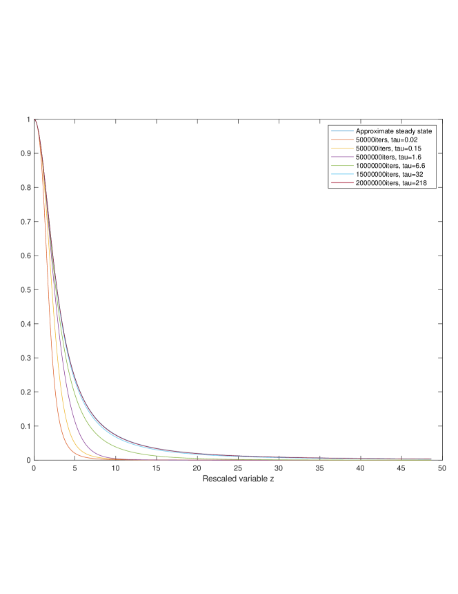
Figure 1: Comparison of the profile to the approximate steady state

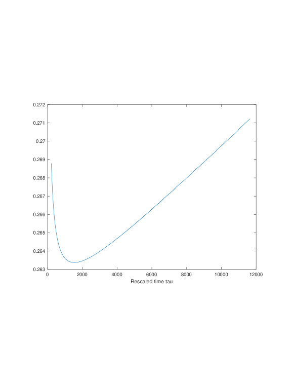
Figure 2: Plot of the residue multiplied by the rescaled time

To see that we can recover the correct convergence rate, we plot $(1/2-\hat{c}_{l})\tau$ and $(\hat{c}_{u}+1)\tau$ in time to see that they indeed converge to the correct constant $5/8$ and $1/4$ respectively and therefore will give the correct log-scaling; see for example indicated by (5). Again for visualization purposes, we only plot for the first $5\times 10^{7}$ iterations and we can see that they converge to the desired constants very fast; see Figure 3.

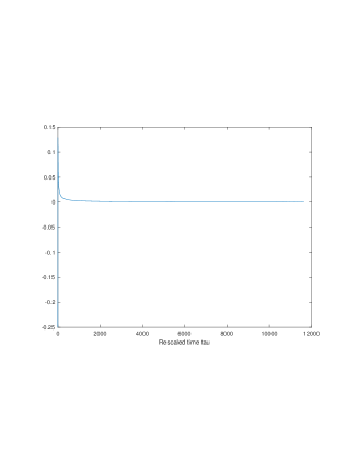
Figure 3: Fitting the law of the normalization constants. Left: $(1/2-\hat{c}_{l})\tau-5/8$ versus $\tau$; right: $(\hat{c}_{u}+1)\tau-1/4$ versus $\tau$.

5.2 2D case

For the 2D example, we choose a nonradial initialization as

$$\hat{u}(0,x,y)=(1+(x^{2}+y^{2})/8+x^{4}/100)^{-1}\,,\quad\hat{C}_{u}(0)=1\,,\quad\lambda_{1}=\lambda_{2}=1\,.$$

At each time step $\tau_{m}$, we first determine the normalization constants as

$$\hat{c}_{u}=-\hat{u}(0,0)-\frac{\lambda_{1}\hat{u}_{xx}(0,0)+\lambda_{2}\hat{u}_{yy}(0,0)}{\hat{u}(0,0)}\,,$$

$$\hat{c}^{1}_{l}=\frac{\hat{c}_{u}}{2}+\hat{u}(0,0)+\frac{\lambda_{1}\hat{u}_{xxxx}(0,0)+\lambda_{2}\hat{u}_{xxyy}(0,0)}{2\hat{u}_{xx}(0,0)}\,,$$

$$\hat{c}^{2}_{l}=\frac{\hat{c}_{u}}{2}+\hat{u}(0,0)+\frac{\lambda_{1}\hat{u}_{xxyy}(0,0)+\lambda_{2}\hat{u}_{yyyy}(0,0)}{2\hat{u}_{yy}(0,0)}\,.$$

Next, we can determine the time step $k$ via the standard numerical stability conditions for a convection-diffusion equation, and then we use the 4-th order Runge-Kutta scheme for the discretization in time and a cubic spline for the discretization in space to evolve the equation

$$\hat{u}_{\tau}=\hat{c}_{u}\hat{u}-\hat{c}^{1}_{l}x\hat{u}_{x}-\hat{c}^{2}_{l}y\hat{u}_{y}+\hat{u}^{2}+\lambda_{1}\hat{u}_{xx}+\lambda_{2}\hat{u}_{yy}\,.$$

Finally, we update our $\lambda_{1}$, $\lambda_{2}$ for time $\tau_{m+1}=\tau_{m}+k$ by a 4-th order Runge-Kutta discretization scheme of the ODE

$$(\log\lambda_{i})_{\tau}=(2\hat{c}^{i}_{l}+\hat{c}_{u})\,,\quad i=1,2\,.$$

We use a fixed nonuniform mesh in space with even symmetry considered, and our computational domain is $[0,4000]$ with $200$ gridpoints in space in each direction. To see that we can recover the correct convergence rate, We plot $R_{i}:=(1/2-\hat{c}_{l}^{i})\tau$ and $R_{u}:=(\hat{c}_{u}+1)\tau$ as a function of $\tau$ after $10^{7}$ iterations to see that they indeed converge to the correct constant $3/4$ and $1/2$ respectively and therefore will give the correct log-scaling; see for example indicated by (22). We can see that they converge to the desired constants very fast; see Figure 4.

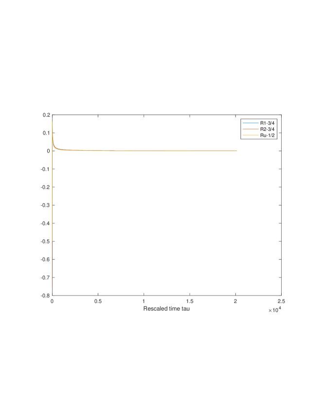
Figure 4: Fitting the law of the normalization constants for 2D.

Acknowledgments. The research was in part supported by NSF Grant DMS-2205590 and the Choi Family Gift Fund. We would like to express our sincere gratitude to Changhe Yang for engaging in valuable discussions, particularly concerning the $n$-dimensional case. Our thanks also go to Peicong Song for insightful conversations during the early stages of this project. Additionally, we are grateful to Dr. Jiajie Chen for his stimulating discussions.

References

- [1] M. Berger and R. V. Kohn. A rescaling algorithm for the numerical calculation of blowing-up solutions. Communications on pure and applied mathematics, 41(6):841–863, 1988.
- [2] J. Bricmont and A. Kupiainen. Universality in blow-up for nonlinear heat equations. Nonlinearity, 7(2):539, 1994.
- [3] T. Buckmaster, S. Shkoller, and V. Vicol. Formation of shocks for 2D isentropic compressible Euler. Communications on Pure and Applied Mathematics, 75(9):2069–2120, 2022.
- [4] J. Chen. Singularity formation and global well-posedness for the generalized Constantin–Lax–Majda equation with dissipation. Nonlinearity, 33(5):2502, 2020.
- [5] J. Chen and T. Y. Hou. Finite time blowup of 2D Boussinesq and 3D Euler equations with velocity and boundary. Communications in Mathematical Physics, 383(3):1559–1667, 2021.
- [6] J. Chen and T. Y. Hou. Stable nearly self-similar blowup of the 2D Boussinesq and 3D Euler equations with smooth data. arXiv preprint arXiv:2210.07191, 2022.
- [7] J. Chen, T. Y. Hou, and D. Huang. On the finite time blowup of the De Gregorio model for the 3D Euler equations. Communications on pure and applied mathematics, 74(6):1282–1350, 2021.
- [8] C. Collot, T.-E. Ghoul, N. Masmoudi, and V. T. Nguyen. Refined description and stability for singular solutions of the 2D Keller-Segel system. Communications on Pure and Applied Mathematics, 75(7):1419–1516, 2022.
- [9] C. Collot, S. Ibrahim, and Q. Lin. Stable singularity formation for the inviscid primitive equations. Annales de l’Institut Henri Poincaré C, 2023.
- [10] T. M. Elgindi. Finite-time singularity formation for solutions to the incompressible Euler equations on . Annals of Mathematics, 194(3):647–727, 2021.
- [11] S. Filippas and R. V. Kohn. Refined asymptotics for the blowup of . Communications on pure and applied mathematics, 45:821–869, 1992.
- [12] S. Filippas and W. Liu. On the blowup of multidimensional semilinear heat equations. In Annales de l’Institut Henri Poincaré C, Analyse non linéaire, volume 10, pages 313–344. Elsevier, 1993.
- [13] M. Herrero and J. Velázquez. Blow–up profiles in one–dimensional semilinear parabolic problems. Communications in partial differential equations, 17(1-2):205–219, 1992.
- [14] T. Y. Hou and Y. Wang. Blowup analysis for a quasi-exact 1D model of 3D Euler and Navier-Stokes. Nonlinearity, 37(3):035001, 2024.
- [15] C. E. Kenig and F. Merle. Global well-posedness, scattering and blow-up for the energy-critical, focusing, non-linear Schrödinger equation in the radial case. Inventiones mathematicae, 166(3):645–675, 2006.
- [16] M. J. Landman, G. C. Papanicolaou, C. Sulem, and P.-L. Sulem. Rate of blowup for solutions of the nonlinear Schrödinger equation at critical dimension. Physical Review A, 38(8):3837, 1988.
- [17] D. McLaughlin, G. Papanicolaou, C. Sulem, and P. Sulem. Focusing singularity of the cubic Schrödinger equation. Physical Review A, 34(2):1200, 1986.
- [18] F. Merle and P. Raphael. The blow-up dynamic and upper bound on the blow-up rate for critical nonlinear Schrödinger equation. Annals of mathematics, pages 157–222, 2005.
- [19] F. Merle and H. Zaag. Stability of the blow-up profile for equations of the type . Duke Math. J, 86(1):143–195, 1997.
- [20] P. Quittner and P. Souplet. Superlinear parabolic problems. Springer, 2019.
- [21] P. Raphaël and R. Schweyer. On the stability of critical chemotactic aggregation. Mathematische Annalen, 359:267–377, 2014.
- [22] A. Soffer. Soliton dynamics and scattering. In International congress of mathematicians, volume 3, pages 459–471, 2006.
- [23] A. Soffer and M. I. Weinstein. Multichannel nonlinear scattering for nonintegrable equations. Communications in mathematical physics, 133:119–146, 1990.
- [24] J. Velázquez. Higher dimensional blow up for semilinear parabolic equations. Communications in partial differential equations, 17(9-10):1567–1596, 1992.
- [25] M. I. Weinstein. Modulational stability of ground states of nonlinear schrödinger equations. SIAM journal on mathematical analysis, 16(3):472–491, 1985.
- [26] W. W. Wong. Some notes on weighted Sobolev spaces. https://qnlw.info/post/weighted-sobolev-spaces-202102/, 2021.