Low-Resource Named Entity Recognition with Cross-Lingual, Character-Level Neural Conditional Random Fields

Abstract

Low-resource named entity recognition is still an open problem in NLP. Most state-of-the-art systems require tens of thousands of annotated sentences in order to obtain high performance. However, for most of the world’s languages, it is unfeasible to obtain such annotation. In this paper, we present a transfer learning scheme, whereby we train character-level neural CRFs to predict named entities for both high-resource languages and low-resource languages jointly. Learning character representations for multiple related languages allows transfer among the languages, improving $F_{1}$ by up to 9.8 points over a log-linear CRF baseline.

author=ryan,color=violet!40,size=,fancyline,caption=,]Add numbers to all equations in the camera ready.

1 Introduction

Named entity recognition (NER) presents a challenge for modern machine learning, wherein a learner must deduce which word tokens refer to people, locations and organizations (along with other possible entity types). The task demands that the learner generalize from limited training data and to novel entities, often in new domains. Traditionally, state-of-the-art NER models have relied on hand-crafted features that pick up on distributional cues as well as portions of the word forms themselves. In the past few years, however, neural approaches that jointly learn their own features have surpassed the feature-based approaches in performance. Despite their empirical success, neural networks have remarkably high sample complexity and still only outperform hand-engineered feature approaches when enough supervised training data is available, leaving effective training of neural networks in the low-resource case a challenge.

For most of the world’s languages, there is a very limited amount of training data for NER; CoNLL—the standard dataset in the field—only provides annotations for 4 languages Tjong Kim Sang (2002); Tjong Kim Sang and De Meulder (2003). Creating similarly sized datasets for other languages has a prohibitive annotation cost, making the low-resource case an important scenario. To get around this barrier, we develop a cross-lingual solution: given a low-resource target language, we additionally offer large amounts of annotated data in a language that is genetically related to the target language. We show empirically that this improves the quality of the resulting model.

In terms of neural modeling, we introduce a novel neural conditional random field (CRF) for cross-lingual NER that allows for cross-lingual transfer by extracting character-level features using recurrent neural networks, shared among multiple languages and; this tying of parameters enables cross-lingual abstraction. With experiments on 15 languages, we confirm that feature-based CRFs outperform the neural methods consistently in the low-resource training scenario. However, with the addition of cross-lingual information, the tables turn and the neural methods are again on top, demonstrating that cross-lingual supervision is a viable method to reduce the training data state-of-the-art neural approaches require.

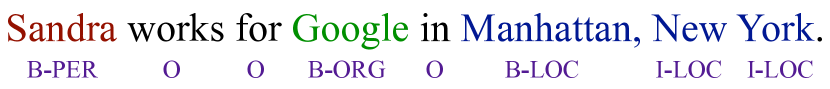
Figure 1: Example of an English sentence annotated with its typed named entities.

2 Neural Conditional Random Fields

Named entity recognition is typically framed as a sequence labeling task using the bio scheme Ramshaw and Marcus (1995); Baldwin (2009), i.e., given an input sentence, the goal is to assign a label to each token: b if the token is the beginning of an entity, or i if the token is inside an entity, or o if the token is outside an entity (see Fig. 1). Following convention, we focus on person (per), location (loc), organization (org), and miscellaneous (misc) entity types, resulting in 9 tags: {b-org, i-org, b-per, i-per, b-loc, i-loc, b-misc, i-misc}.

Conditional random fields (CRFs), first introduced in Lafferty et al. (2001), generalize the classical maximum entropy models Berger et al. (1996) to distributions over structured objects, and are an effective tool for sequence labeling tasks like NER. We briefly overview the formalism here and then discuss its neural parameterization.

2.1 CRFs: A Cursory Overview

We start with two discrete alphabets $\Sigma$ and $\Delta$. In the case of sentence-level sequence tagging, $\Sigma$ is a set of words (potentially infinite) and $\Delta$ is a set of tags (generally finite; in our case $|\Delta|=9$). Given $\mathbf{t}=t_{1}\cdots t_{n}\in\Delta^{n}$ and $\mathbf{w}=w_{1}\cdots w_{n}\in\Sigma^{n}$, where $n$ is the sentence length. A CRF is a globally normalized conditional probability distribution,

$$p_{{\boldsymbol{\theta}}}(\mathbf{t}\mid\mathbf{w})=\frac{1}{Z_{{\boldsymbol{\theta}}}(\mathbf{w})}\prod_{i=1}^{n}\psi\left(t_{i-1},t_{i},\mathbf{w};{\boldsymbol{\theta}}\right),$$ (1)

where $t_{0}$ is distinguished beginning-of-tagging symbol, $\psi\left(t_{i-1},t_{i},\mathbf{w};{\boldsymbol{\theta}}\right)\geq 0$ is an arbitrary non-negative potential function that we take to be a parametric function of the parameters ${\boldsymbol{\theta}}$ and the partition function $Z_{{\boldsymbol{\theta}}}(\mathbf{w})$ is the sum over all taggings of length $n$.

So how do we choose $\psi\left(t_{i-1},t_{i},\mathbf{w};{\boldsymbol{\theta}}\right)$? We discuss two alternatives, which we will compare experimentally in § 5.

2.2 Log-Linear Parameterization

Traditionally, computational linguists have cosnidered a simple log-linear parameterization, i.e.,

$$\psi\left(t_{i-1},t_{i},\mathbf{w};{\boldsymbol{\theta}}\right)=\exp\Big{(}{\boldsymbol{\eta}}^{\top}{\boldsymbol{f}}(t_{i-1},t_{i},\mathbf{w})\Big{)}$$ (2)

where ${\boldsymbol{\eta}}\in\mathbb{R}^{d}$ and the user defines a feature function ${\boldsymbol{f}}:\Delta\times\Delta\times\Sigma^{n}\to\mathbb{R}^{d}$ that extracts relevant information from the adjacent tags $t_{i-1}$ and $t_{i}$ and the sentence $\mathbf{w}$. In this case, the model’s parameters are ${\boldsymbol{\theta}}=\{{\boldsymbol{\eta}}\}$. Common binary features include word form features, e.g., does the word at the $i^{\text{th}}$ position end in -ation?, and contextual features, e.g., is the word next to $(i\!-\!1)^{\text{th}}$ word the? These binary features are conjoined with other indicator features, e.g., is the $i^{\text{th}}$ tag i-loc? We refer the reader to Sha and Pereira (2003) for standard CRF feature functions employed in NER, which we use in this work.author=ryan,color=violet!40,size=,fancyline,caption=,]Double check that this is true. The log-linear parameterization yields a convex objective and is extremely efficient to compute as it only involves a sparse dot product, but the representational power of model depends fully on the quality of the features the user selects.

2.3 (Recurrent) Neural Parameterization

Modern CRFs, however, try to obviate the hand-selection of features through deep, non-linear parameterizations of $\psi\left(t_{i-1},t_{i},\mathbf{w};{\boldsymbol{\theta}}\right)$. This idea is far from novel and there have been numerous attempts in the literature over the past decade to find effective non-linear parameterizations Peng et al. (2009); Do and Artières (2010); Collobert et al. (2011); Vinel et al. (2011); Fujii et al. (2012). Until recently, however, it was not clear that these non-linear parameterizations of CRFs were worth the non-convexity and the extra computational cost. Indeed, on neural CRFs, Wang and Manning (2013) find that “a nonlinear architecture offers no benefits in a high-dimensional discrete feature space.”

However, recently with the application of long short-term memory (LSTM; Hochreiter and Schmidhuber, 1997) recurrent neural networks (RNNs; Elman, 1990) to CRFs, it has become clear that neural feature extractors are superior to the hand-crafted approaches Huang et al. (2015); Lample et al. (2016); Ma and Hovy (2016). As our starting point, we build upon the architecture of Lample et al. (2016), which is currently competitive with the state of the art for NER.

$$\psi(t_{i-1},t_{i}, \mathbf{w};\left.{\boldsymbol{\theta}}\right)=$$ (3)

$$\exp\left(a(t_{i-1},t_{i})\!+\!\mathbf{o}(t_{i})^{\top}\mathbf{W}\,\mathbf{s}(\mathbf{w})_{i}\right),$$

where $a(t_{i-1},t_{i})$ is the weight of transitioning from $t_{i-1}$ to $t_{i}$ and $\mathbf{o}(t_{i})\in\mathbb{R}^{r_{1}}$, $\mathbf{s}(\mathbf{w})_{i}\in\mathbb{R}^{r_{2}}$ and $\mathbf{W}\in\mathbb{R}^{r_{1}\times r_{2}}$ are the output tag embedding, the word embedding for the $i^{\text{th}}$ word embedding and an interaction matrix, respectively. We define sentence’s embeddings as the concatenation of an LSTM run forward and backward, i.e.,

$$\mathbf{s}(\mathbf{w})=\left[\overrightarrow{\text{LSTM}_{{\boldsymbol{\theta}}^{\prime}}}({\boldsymbol{\omega}});\,\overleftarrow{\text{LSTM}_{{\boldsymbol{\theta}}^{\prime}}}({\boldsymbol{\omega}})\right].$$ (4)

We denote the embedding for the $i^{\text{th}}$ word in this sentence is $\mathbf{s}(\mathbf{w})_{i}$. The input vector ${\boldsymbol{\omega}}=[\omega_{1},\ldots,\omega_{|\mathbf{w}|}]$ to this BiLSTM is a vector of embeddings: we define

$$\omega_{i}=\left[\text{LSTM}_{{\boldsymbol{\theta}}^{\prime\prime}}\left(c_{1}\cdots c_{|w_{i}|}\right);\,\mathbf{e}(w_{i})\right],$$ (5)

where $c_{1}\cdots c_{|w_{i}|}$ are the characters in word $w_{i}$. In other words, we run an LSTM over the character stream and concatenate it with a word embedding for each type. Now, the parameters ${\boldsymbol{\theta}}$, ${\boldsymbol{\theta}}^{\prime}$ and ${\boldsymbol{\theta}}^{\prime\prime\prime}$ are the set of all the LSTM parameters and other embeddings.

3 Cross-Lingual Extensions

One of the most striking features of neural networks is their ability to abstract general representations across many words. Our question is: can neural feature-extractors abstract the notion of a named entity across similar languages? For example, if we train a character-level neural CRF on several of the highly related Romance languages, can our network learn a general representation of the entities in these languages?

3.1 Cross-Lingual Architecture

We now describe our novel cross-lingual architecture. Given a language label $\ell$, we want to create a language-specific CRF $p_{{\boldsymbol{\theta}}}(\mathbf{t}\mid\mathbf{w},\ell)$ with potential:

$$\psi\Big{(}t_{i-1},t_{i}, \mathbf{w},\ell;{\boldsymbol{\theta}}\Big{)}=\exp\left(a(t_{i-1},t_{i})+\right.$$ (6)

$$\mathbf{u}^{\top}\!\tanh(\mathbf{U}\left.\left[\right.\mathbf{s}(\mathbf{w})_{i};\,\mathbf{l}(\ell)\left.\right]+\mathbf{b})\right),$$

$\mathbf{l}(\ell)\in\mathbb{R}^{r_{3}}$ is an embedding of the language ID, itself, and $\mathbf{U}\in\mathbb{R}^{q\times r_{2}+r_{3}}$ is a projection matrix, $\mathbf{u}\in\mathbb{R}^{q}$ is a vector, and $a(\cdot,\cdot)$ is a transition weight for each pair of tags. Importantly, we share some parameters across languages: the transitions $a()$ between tags and the character-level neural networks that discover what a form looks like. Recall $\mathbf{s}(\mathbf{w})$ is defined in Eq. 4 and Eq. 5. The character encoder $\text{LSTM}_{{\boldsymbol{\theta}}}\left(c_{1}\cdots c_{|w_{i}|}\right)$ is shared cross-lingually while $\mathbf{e}(w_{i})$ is language-specific.

Now, given a low-resource target language $\tau$ and a source language $\sigma$ (potentially, a set of $m$ high-resource source languages $\{\sigma_{i}\}_{i=1}^{m}$). We consider the following log-likelihood objective

$${\cal L}\left({\boldsymbol{\theta}}\right) =\!\!\sum_{(\mathbf{t},\mathbf{w})\in{\cal D}_{\tau}}\!\!\!\!\!\log p_{{\boldsymbol{\theta}}}\left(\mathbf{t}\mid\mathbf{w},\tau\right)+$$ (7)

$$\hskip 56.9055pt\mu\cdot\!\!\!\!\!\!\sum_{(\mathbf{t},\mathbf{w})\in{\cal D}_{\sigma}}\!\!\!\!\!\log p_{{\boldsymbol{\theta}}}\left(\mathbf{t}\mid\mathbf{w},\sigma\right),$$

where $\mu>0$ is a trade-off parameter, ${\cal D}_{\tau}$ is the set of training examples for the target language and ${\cal D}_{\sigma}$ is the set of training data for the source language $\sigma$. In the case of multiple source languages, we add a summand to the set of source languages used, in which case set have multiple training sets ${\cal D}_{\sigma_{i}}$.

In the case of the log-linear parameterization, we simply add a language-specific atomic feature for the language-id, drawing inspiration from Daumé III (2007)’s approach for domain adaption. We then conjoin this new atomic feature with the existing feature templates, doubling the number of feature templates: the original and the new feature template conjoined with the language ID.

Language Code Family Branch Galician gl Indo-European Romance Catalan cl Indo-European Romance French fr Indo-European Romance Italian it Indo-European Romance Romanian ro Indo-European Romance Spanish es Indo-European Romance West Frisian fy Indo-European Germanic Dutch nl Indo-European Germanic Tagalog tl Austronesian Philippine Cebuano ceb Austronesian Philippine Ukrainian uk Indo-European Slavic Russian ru Indo-European Slavic Marathi mr Indo-European Indo-Aryan Hindi hi Indo-European Indo-Aryan Urdu ur Indo-European Indo-Aryan

Table 1: List of the languages used in our experiments with their ISO 639-1 codes, family and the branch in that family.

	languages	low-resource ($|{\cal D}_{\tau}|=100$)			high-resource ($|{\cal D}_{\tau}|=10000$)
$\tau$	$\sigma_{i}$	log-linear	neural	${\boldsymbol{\Delta}}$	log-linear	neural	${\boldsymbol{\Delta}}$
gl	—	$57.64$	$49.19$	${\color[rgb]{1,0,0}-8.45}$	$87.23$	$89.42$	${\color[rgb]{0,0,1}+2.19}$
gl	es	$71.46$	$76.40$	${\color[rgb]{0,0,1}+4.94}$	$87.50$	$89.46$	${\color[rgb]{0,0,1}+1.96}$
gl	ca	$67.32$	$75.40$	${\color[rgb]{0,0,1}+8.08}$	$87.40$	$89.32$	${\color[rgb]{0,0,1}+1.92}$
gl	it	$63.81$	$70.93$	${\color[rgb]{0,0,1}+7.12}$	$87.34$	$89.50$	${\color[rgb]{0,0,1}+2.16}$
gl	fr	$58.22$	$68.02$	${\color[rgb]{0,0,1}+9.80}$	$87.92$	$89.38$	${\color[rgb]{0,0,1}+1.46}$
gl	ro	$59.23$	$67.76$	${\color[rgb]{0,0,1}+8.44}$	$87.24$	$89.19$	${\color[rgb]{0,0,1}+1.95}$
fy	—	$62.71$	$58.43$	${\color[rgb]{1,0,0}-4.28}$	$90.42$	$91.03$	${\color[rgb]{0,0,1}+0.61}$
fy	nl	$68.15$	$72.12$	${\color[rgb]{0,0,1}+3.97}$	$90.94$	$91.01$	${\color[rgb]{0,0,1}+0.07}$
tl	—	$58.15$	$56.98$	${\color[rgb]{1,0,0}-1.17}$	$74.24$	$79.03$	${\color[rgb]{0,0,1}+4.79}$
tl	ceb	$75.29$	$81.79$	${\color[rgb]{0,0,1}+6.50}$	$74.02$	$79.51$	${\color[rgb]{0,0,1}+5.48}$
uk	—	$61.40$	$60.65$	${\color[rgb]{1,0,0}-0.75}$	$85.63$	$87.39$	${\color[rgb]{0,0,1}+1.75}$
uk	ru	$70.94$	$76.74$	${\color[rgb]{0,0,1}+5.80}$	$86.01$	$87.42$	${\color[rgb]{0,0,1}+1.41}$
mr	—	$42.76$	$39.02$	${\color[rgb]{1,0,0}-3.73}$	$70.98$	$74.95$	${\color[rgb]{0,0,1}+4.86}$
mr	hi	$54.25$	$60.92$	${\color[rgb]{0,0,1}+6.67}$	$70.45$	$74.49$	${\color[rgb]{0,0,1}+4.04}$
mr	ur	$49.32$	$58.92$	${\color[rgb]{0,0,1}+9.60}$	$70.75$	$74.81$	${\color[rgb]{0,0,1}+4.07}$

Table 2: Results comparing the log-linear and neural CRFs in various settings. We compare the log-linear linear and the neural CRF in the low-resource transfer setting. The difference (${\boldsymbol{\Delta}}$) is blue when positive and red when negative.

4 Related Work

We divide the discussion of related work topically.

Character-Level Neural Networks.

In recent years, many authors have incorporated character-level information into taggers using neural networks, e.g., dos Santos and Zadrozny (2014) employed a convolutional network for part-of-speech tagging in morphologically rich languages and Ling et al. (2015) a LSTM for a myriad of different tasks. Relatedly, Chiu and Nichols (2016) approached NER with character-level LSTMs, but without using a CRF. Our work firmly builds upon this in that we, too, compactly summarize the word form with a recurrent neural component.

Neural Transfer Schemes.

Previous work has also performed transfer learning using neural networks. The novelty of our work lies in the cross-lingual transfer. For example, Peng and Dredze (2017) and Yang et al. (2017), similarly oriented concurrent papers, focus on domain adaptation within the same language. While this is a related problem, cross-lingual transfer is much more involved since the morphology, syntax and semantics change more radically between two languages than between domains.

Projection-based Transfer Schemes.

Projection is a common approach to tag low-resource languages. The strategy involves annotating one side of bitext with a tagger for a high-resource language and then project the annotation the over the bilingual alignments obtained through unsupervised learning Och and Ney (2003). Using these projected annotations as weak supervision, one then trains a tagger in the target language. This line of research has a rich history, starting with Yarowsky and Ngai (2001). For a recent take, see Wang and Manning (2014) for projecting NER from English to Chinese. We emphasize that projection-based approaches are incomparable to our proposed method as they make an additional bitext assumption, which is generally not present in the case of low-resource languages.

5 Experiments

Fundamentally, we want to show that character-level neural CRFs are capable of generalizing the notion of an entity across related languages. To get at this, we compare a linear CRF (see § 2.2) with standard feature templates for the task and a neural CRF (see § 2.3). We further compare three training set-ups: low-resource, high-resource and low-resource with additional cross-lingual data for transfer. Given past results in the literature, we expect linear CRF to dominate in the low-resource settings, the neural CRF to dominate in the high-resource setting. The novelty of our paper lies in the consideration of the low-resource with transfer case: we show that neural CRFs are better at transferring entity-level abstractions cross-linguistically.

5.1 Data

We experiment on 15 languages from the cross-lingual named entity dataset described in Pan et al. (2017). We focus on 5 typologically diverse target languages: Galician, West Frisian, Ukrainian, Marathi and Tagalog. As related source languages, we consider Spanish, Catalan, Italian, French, Romanian, Dutch, Russian, Cebuano, Hindi and Urdu. For the language code abbreviations and linguistic families, see Tab. 1. For each of the target languages, we emulate a truly low-resource condition, creating a 100 sentence split for training. We then create a 10000 sentence superset to be able to compare to a high-resource condition in those same languages. For the source languages, we only created a 10000 sentence split. We also create disjoint validation and test splits, of 1000 sentences each. author=kevin,color=violet!40,size=,fancyline,caption=,inline,]In Table 2, it’s not clear for cross-lingual settings whether the source data uses 10000 sentences or 100 sentences. Clarify.

5.2 Results

The linear CRF is trained using L-BFGS author=ryan,color=violet!40,size=,fancyline,caption=,]add citation until convergence using the CRF suite toolkit. We train our neural CRF for 100 epochs using AdaDelta Zeiler (2012) with a learning rate of $1.0$. The results are reported in Tab. 2. To understand the table, take the target language ($\tau$) Galician. In terms of $F_{1}$, while the neural CRF outperforms the log-linear CRF in the high-resource setting ($89.42$ vs. $87.23$), it performs poorly in the low-resource setting ($49.19$ vs. $56.64$); when we add in a source language ($\sigma_{i}$) such as Spanish, $F_{1}$ increases to $76.40$ for the neural CRF and $71.46$ for the log-linear CRF. The trend is similar for other source languages, such as Catalan ($75.40$) and Italian ($70.93$).

Overall, we observe three general trends. i) In the monolingual high-resource case, the neural CRF outperforms the log-linear CRF. ii) In the low-resource case, the log-linear CRF outperforms the neural CRF. iii) In the transfer case, the neural CRF wins, however, indicating that our character-level neural approach is truly better at generalizing cross-linguistically in the low-resource case (when we have little target language data), as we hoped. In the high-resource case (when we have a lot of target language data), the transfer learning has little to no effect. We conclude that our cross-lingual neural CRF is a viable method for the transfer of NER. However, there is still a sizable gap between the neural CRF trained on 10000 target sentences and the transfer case (100 target and 10000 source), indicating there is still room for improvement.

author=kevin,color=violet!40,size=,fancyline,caption=,]Do we have some example character embeddings that worked well cross-lingually? Is it possible to find at least one example quickly?

author=kevin,color=violet!40,size=,fancyline,caption=,]Can we find a breakdown of F1 or precision/recall scores by entity type and see which one is helped most by cross-lingual (if there’s any trend)?

author=ryan,color=violet!40,size=,fancyline,caption=,]Consider multi-source and script transfer (already done with Urdu)

6 Conclusion

We have investigated the task of cross-lingual transfer in low-resource named entity recognition using neural CRFs with experiments on 15 typologically diverse languages. Overall, we show that direct cross-lingual transfer is an option for reducing sample complexity for state-of-the-art architectures. In the future, we plan to investigate how exactly the networks manage to induce a cross-lingual entity abstraction.

References

- Baldwin (2009) Breck Baldwin. 2009. Coding chunkers as taggers: IO, BIO, BMEWO, and BMEWO+. http://bit.ly/2xRo8Ni.
- Berger et al. (1996) Adam L. Berger, Vincent J. Della Pietra, and Stephen A. Della Pietra. 1996. A maximum entropy approach to natural language processing. Computational Linguistics, 22(1):39–71.
- Chiu and Nichols (2016) Jason Chiu and Eric Nichols. 2016. Named entity recognition with bidirectional LSTM-CNNs. Transactions of the Association of Computational Linguistics, 4:357–370.
- Collobert et al. (2011) Ronan Collobert, Jason Weston, Léon Bottou, Michael Karlen, Koray Kavukcuoglu, and Pavel Kuksa. 2011. Natural language processing (almost) from scratch. Journal of Machine Learning Research, 12(Aug):2493–2537.
- Daumé III (2007) Hal Daumé III. 2007. Frustratingly easy domain adaptation. In Proceedings of the 45th Annual Meeting of the Association of Computational Linguistics, pages 256–263, Prague, Czech Republic. Association for Computational Linguistics.
- Do and Artières (2010) Trinh-Minh-Tri Do and Thierry Artières. 2010. Neural conditional random fields. In Proceedings of the Thirteenth International Conference on Artificial Intelligence and Statistics, pages 177–184.
- Elman (1990) Jeffrey L. Elman. 1990. Finding structure in time. Cognitive Science, 14(2):179–211.
- Fujii et al. (2012) Yasuhisa Fujii, Kazumasa Yamamoto, and Seiichi Nakagawa. 2012. Deep-hidden conditional neural fields for continuous phoneme speech recognition. In Proceedings of the International Workshop of Statistical Machine Learning for Speech Processing (IWSML).
- Hochreiter and Schmidhuber (1997) Sepp Hochreiter and Jürgen Schmidhuber. 1997. Long short-term memory. Neural Computation, 9(8):1735–1780.
- Huang et al. (2015) Zhiheng Huang, Wei Xu, and Kai Yu. 2015. Bidirectional LSTM-CRF models for sequence tagging. arXiv preprint arXiv:1508.01991.
- Lafferty et al. (2001) John D. Lafferty, Andrew McCallum, and Fernando C. N. Pereira. 2001. Conditional random fields: Probabilistic models for segmenting and labeling sequence data. In Proceedings of the Eighteenth International Conference on Machine Learning (ICML), pages 282–289.
- Lample et al. (2016) Guillaume Lample, Miguel Ballesteros, Sandeep Subramanian, Kazuya Kawakami, and Chris Dyer. 2016. Neural architectures for named entity recognition. In Proceedings of the 2016 Conference of the North American Chapter of the Association for Computational Linguistics: Human Language Technologies, pages 260–270, San Diego, California. Association for Computational Linguistics.
- Ling et al. (2015) Wang Ling, Chris Dyer, Alan W Black, Isabel Trancoso, Ramon Fermandez, Silvio Amir, Luis Marujo, and Tiago Luis. 2015. Finding function in form: Compositional character models for open vocabulary word representation. In Proceedings of the 2015 Conference on Empirical Methods in Natural Language Processing, pages 1520–1530, Lisbon, Portugal. Association for Computational Linguistics.
- Ma and Hovy (2016) Xuezhe Ma and Eduard Hovy. 2016. End-to-end sequence labeling via bi-directional LSTM-CNNs-CRF. In Proceedings of the 54th Annual Meeting of the Association for Computational Linguistics (Volume 1: Long Papers), pages 1064–1074. Association for Computational Linguistics.
- Och and Ney (2003) Franz Josef Och and Hermann Ney. 2003. A systematic comparison of various statistical alignment models. Computational Linguistics, 29(1):19–51.
- Pan et al. (2017) Xiaoman Pan, Boliang Zhang, Jonathan May, Joel Nothman, Kevin Knight, and Heng Ji. 2017. Cross-lingual name tagging and linking for 282 languages. In Proceedings of the 55th Annual Meeting of the Association for Computational Linguistics (Volume 1: Long Papers), Vancouver, Canada. Association for Computational Linguistics.
- Peng et al. (2009) Jian Peng, Liefeng Bo, and Jinbo Xu. 2009. Conditional neural fields. In Advances in Neural Information Processing Systems (NIPS), pages 1419–1427.
- Peng and Dredze (2017) Nanyun Peng and Mark Dredze. 2017. Multi-task domain adaptation for sequence tagging. In Proceedings of the 2nd Workshop on Representation Learning for NLP, Vancouver, Canada. Association for Computational Linguistics.
- Ramshaw and Marcus (1995) Lance A. Ramshaw and Mitchell P. Marcus. 1995. Text chunking using transformation-based learning. In Proceedings of the 3rd ACL Workshop on Very Large Corpora, pages 82–94. Association for Computational Linguistics.
- dos Santos and Zadrozny (2014) Cicero Nogueira dos Santos and Bianca Zadrozny. 2014. Learning character-level representations for part-of-speech tagging. In International Conference on Machine Learning (ICML), volume 32, pages 1818–1826.
- Sha and Pereira (2003) Fei Sha and Fernando C. N. Pereira. 2003. Shallow parsing with conditional random fields. In Human Language Technology Conference of the North American Chapter of the Association for Computational Linguistics, HLT-NAACL 2003.
- Tjong Kim Sang (2002) Erik F. Tjong Kim Sang. 2002. Introduction to the CoNLL-2002 shared task: Language-independent named entity recognition. In COLING-02: The 6th Conference on Natural Language Learning 2002 (CoNLL-2002).
- Tjong Kim Sang and De Meulder (2003) Erik F. Tjong Kim Sang and Fien De Meulder. 2003. Introduction to the CoNLL-2003 shared task: Language-independent named entity recognition. In Proceedings of the Seventh Conference on Natural Language Learning at HLT-NAACL 2003, pages 142–147.
- Vinel et al. (2011) Antoine Vinel, Trinh-Minh-Tri Do, and Thierry Artières. 2011. Joint optimization of hidden conditional random fields and non linear feature extraction. In 2011 International Conference on Document Analysis and Recognition (ICDAR), pages 513–517. IEEE.
- Wang and Manning (2013) Mengqiu Wang and Christopher D. Manning. 2013. Effect of non-linear deep architecture in sequence labeling. In Proceedings of the Sixth International Joint Conference on Natural Language Processing, pages 1285–1291, Nagoya, Japan. Asian Federation of Natural Language Processing.
- Wang and Manning (2014) Mengqiu Wang and Christopher D. Manning. 2014. Cross-lingual pseudo-projected expectation regularization for weakly supervised learning. Transactions of the Association for Computational Linguistics.
- Yang et al. (2017) Zhilin Yang, Ruslan Salakhutdinov, and William W. Cohen. 2017. Transfer learning for sequence tagging with hierarchical recurrent networks. In International Conference on Learning Representations (ICLR).
- Yarowsky and Ngai (2001) David Yarowsky and Grace Ngai. 2001. Inducing multilingual POS taggers and NP brackets via robust projection across aligned corpora. In Human Language Technology Conference of the North American Chapter of the Association for Computational Linguistics, HLT-NAACL 2001.
- Zeiler (2012) Matthew D. Zeiler. 2012. ADADELTA: An adaptive learning rate method. arXiv preprint arXiv:1212.5701.