A Machine Learning Approach for Optimizing Hybrid Quantum Noise Clusters for Gaussian Quantum Channel Capacity

Abstract

This research contributes to the advancement of quantum communication by visualizing hybrid quantum noise in higher dimensions and optimizing the capacity of the quantum channel by using machine learning (ML). Employing the expectation maximization (EM) algorithm, the quantum channel parameters are iteratively adjusted to estimate the channel capacity, facilitating the categorization of quantum noise data in higher dimensions into a finite number of clusters. In contrast to previous investigations that represented the model in lower dimensions, our work describes the quantum noise as a Gaussian Mixture Model (GMM) with mixing weights derived from a Poisson distribution. The objective was to model the quantum noise using a finite mixture of Gaussian components while preserving the mixing coefficients from the Poisson distribution. Approximating the infinite Gaussian mixture with a finite number of components makes it feasible to visualize clusters of quantum noise data without modifying the original probability density function. By implementing the EM algorithm, the research fine-tuned the channel parameters, identified optimal clusters, improved channel capacity estimation, and offered insights into the characteristics of quantum noise within an ML framework.

=-15pt

I Introduction

Quantum communication, an expanding area that merges quantum mechanics and information theory, has the potential for unmatched security and effectiveness in transmitting information. In addition, it can address issues related to data and information security. Quantum communication entails transferring quantum information through a quantum channel among various entities using quantum-mechanical elements like photons. It facilitates functions such as quantum cryptography [1], quantum teleportation [2], and quantum networks [3]. The inherent benefits of quantum communication are closely connected to addressing issues related to quantum noise, which arises from the interaction of quantum systems with their surroundings or during the measurement process and can significantly hinder the accuracy and dependability of quantum information transmission. Due to the high sensitivity of quantum systems to external interferences, quantum noise can result in the degradation of coherence and entanglement, which are vital aspects of quantum communication [4]. Approaches such as quantum error correction and the utilization of decoherence-free subspaces are aimed at maintaining the integrity of quantum information in the presence of inevitable noise [5].

A thorough understanding of the noise that impacts these systems is essential for accurately modeling and assessing their performance in quantum technologies. Hybrid quantum-classical noise, which combines classical Additive White Gaussian Noise (AWGN) and quantum Poisson noise, plays a crucial role in this context. Quantum systems are inherently susceptible to quantum noise, like Poisson noise, due to the discrete nature of light and matter [6]. On the contrary, classical noise affects classical systems, including AWGN, due to thermal fluctuations and electronic components. By incorporating both forms of noise into a hybrid model, the complete range of disturbances can be captured in systems that bridge the quantum and classical domains [7]. Adopting a hybrid noise model enables a more accurate assessment of system performance, covering error rates, information capacity, and security analyses [8][9]. Particularly, it is critical for optimizing the design and operation of quantum technology, significantly enhancing the sensitivity and resolution of quantum sensing [10] and imaging. Consequently, simulations that consider both quantum Poisson noise and classical AWGN provide realistic testing environments essential for developing quantum error correction techniques and creating robust quantum protocols resistant to noise [11].

Quantum noise can disrupt quantum entanglement, leading to decoherence and deterioration of entanglement, a process that poses significant challenges for quantum communication and computing [12, 13]. Machine learning (ML) algorithms can play a crucial role in the more efficient generation and detection of entangled states, which is vital for various quantum communication protocols [14], [15], thus improving the performance of quantum communication systems. To illustrate how ML algorithms can enhance the generation of high-dimensional entangled states with better fidelity and efficiency, a hybrid approach has been suggested. This approach combines quantum control techniques with ML algorithms to optimize the process of generating entanglement [16]. Generative ML models can be utilized for quantum state tomography, including identifying entangled states. This approach provides a more efficient and precise method for characterizing quantum states, especially those related to entanglement [17], [18], [19].

ML methods could have a crucial impact on improving the estimation and optimization of quantum channel parameters, error correction, resource allocation, and quantum information transmission. Progress has been notable in quantum communication technology for free-space satellites [20]. However, challenges related to quantum repeaters for long-distance quantum communications still need to be addressed to establish a global quantum network [21, 22]. Free-space quantum communication channels have encountered difficulties such as loss in the quantum channel, security issues, and limited data rates [22]. Conventional ML techniques offer a valuable approach to characterizing the features of free-space quantum channels [20]. In a recent study [23], supervised ML was employed to forecast the atmospheric strength of a free-space quantum channel.

Estimating parameters in Gaussian quantum channels is a crucial task that involves identifying and optimizing variables essential for transmitting quantum states. A Gaussian Mixture Model (GMM) represents a probability density function by a weighted sum of Gaussian component densities, providing a flexible representation of non-Gaussian densities. With sufficient components, GMMs can approximate any smooth function with arbitrary accuracy, making them suitable for representing multivariate densities in practical applications [24], [25]. The expectation maximization (EM) algorithm [26], [27] being a robust iterative technique efficiently estimates the quantum channel parameters maximizing the likelihood function. Maximum likelihood significantly improves Gaussian quantum channels by reducing noise and errors to enhance performance using updated parametric values. Focusing on Gaussian states and operations, these channels can benefit from ML models trained to forecast their evolution, thus refining quantum communication protocols [28]. In hybrid Quantum-Classical systems, ML aids in integrating Gaussian channels, facilitating the efficient exchange of classical and quantum information. ML techniques are essential for characterizing Gaussian quantum channels, enabling the identification of crucial attributes such as noise properties and entanglement effects, as well as detecting anomalies indicating external interference or unexpected noise [29]. GMMs further elucidate the hybrid quantum-classical noise model of these channels [7].

TABLE I: Notation

$tr$	The trace of a matrix
$\mathbf{T(\cdot)}$	Trace-preserving map $\mathbf{T}$
$\mathbf{A}^{\dagger}$	The adjoint of matrix $\mathbf{A}$
${\mathbf{A}}^{T}$	The transpose of matrix $\mathbf{A}$
$\nu^{*}$	The complex conjugate of $\nu$
$\otimes$	The tensor product
$\mathcal{N}$	Gaussian density
$\ket{\cdot}$	The ket
$\bra{\cdot}$	The bra
$|\cdot|$	The norm

Figure 1: The flowchart of the research.

Furthermore, ML optimizes the preparation of the Gaussian state, enhancing transmission fidelity through precise squeezing and displacement [10],[6]. As parametric representations of the probability distribution of continuous measurements, these models are adept at forming smooth approximations of arbitrarily shaped densities, which is crucial for precise and reliable estimation of channel characteristic. This enhances quantum state transmission fidelity and performance. The iterative EM algorithm for calculating the Maximum A Posteriori (MAP) [30], [31] estimation of GMM parameters from training data is a widely accepted technique among researchers. This method significantly aids in the estimation of parameters for Gaussian quantum channels, optimizing the transmission of quantum states [32].

A mathematical model introduced in [7] tackles hybrid quantum-classical noise, combining quantum Poisson noise with classical white Gaussian noise. Our study advances quantum communication by integrating ML techniques to manage hybrid quantum noise. Utilizing an iterative ML algorithm, we optimize quantum channel parameters for precise capacity estimation and enhanced quantum noise visualization in higher dimensions. Our method defines the quantum noise model as a GMM, transforming it from an infinite to a finite mixture while preserving the original probability density function. Through the EM algorithm, we fine-tune channel parameters, yielding improved capacity estimates. This innovative ML approach enhances our comprehension of quantum noise’s impact on channel capacity, underscoring ML’s potential in quantum communication advancement. In essence, the critical contributions of this study can be summarized in three main aspects:

• Our framework utilizes an iterative ML algorithm to dynamically adjust the quantum channel parameters. This iterative process improves the accuracy of estimating the quantum channel capacity. It facilitates the visualization of the quantum noise model in higher dimensions. Initially, based on the hybrid quantum noise model represented as a multivariate GMM that comprises an infinite combination of multivariate Gaussian elements with mixing weights obtained from a Poisson distribution, we have introduced a technique to transform it into a finite mixture of multivariate Gaussians while retaining the original Poisson mixing coefficients. This method aims to simplify the complexity of the infinite mixture into a more manageable structure without compromising the integrity of the probability density function (p.d.f.).

• We employ the EM algorithm to enhance the quantum channel parameters and detect the best quantum noise groups. This improves the parameters of the quantum channel and pinpoints optimal data clusters, resulting in a more accurate determination of the quantum channel capacities using signal-to-noise ratios. Comparative evaluation demonstrates that our ML-boosted parameters significantly surpass the original approximations, emphasizing our model’s effectiveness.

• Our results reveal a comparative assessment that indicates that the ML-enhanced channel parameters provide better estimations of the quantum channel capacity compared to the initial parameter assumptions. This comparison highlights the efficiency of integrating ML in optimizing quantum communication channels. Moreover, our progress in visualizing quantum noise data clusters in elevated dimensions provides a deep understanding of quantum noise properties, showcasing the strong potential of ML to enhance quantum communication technologies.

Overall, our work demonstrates the powerful use of ML in improving quantum communication technologies, providing new avenues to comprehend and address the issues caused by quantum noise in quantum channels. Please note, a comprehensive list of the notations used throughout this paper is provided in Table LABEL:NoationTable.

II System Model

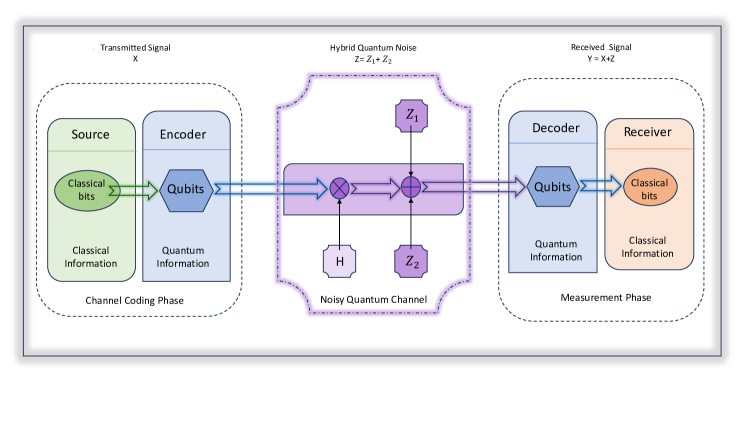
Figure 2: A noisy Quantum Channel: A schematic diagram showing a single quantum link between transmitter and receiver.

II-A Gaussian Quantum Channel Model

A qubit is represented as a linear combination of the basis states $\boldsymbol{\ket{0}}$ and $\boldsymbol{\ket{1}}$, which can be written as: $\boldsymbol{\ket{\psi}}=\alpha\boldsymbol{\ket{0}}+\beta\boldsymbol{\ket{1}}$, where $\alpha,\beta$ are complex numbers such that $|\alpha|^{2}+|\beta|^{2}=1$. This normalization condition ensures that the total probability is 1. The density matrix formalism offers a more general way to describe quantum states, including pure and mixed states. A single-state vector describes a pure state, whereas a mixed state represents a statistical mixture of several state vectors. For a qubit in pure state $\boldsymbol{\ket{\psi}}$, the density matrix $\boldsymbol{\rho}$ is given by

$$\boldsymbol{\rho}=\ket{\boldsymbol{\psi}}\bra{\boldsymbol{\psi}}=\begin{bmatrix}|\alpha|^{2}&\alpha^{*}\beta\\ \alpha\beta^{*}&|\beta|^{2}\end{bmatrix},$$

where $\alpha^{*}$ and $\beta^{*}$ are the complex conjugates of $\alpha$ and $\beta$, respectively. The density matrix for a mixed state, which is a probabilistic mixture of pure states $\boldsymbol{\ket{\psi_{i}}}$ with probabilities $p_{i}$, is given by $\boldsymbol{\rho}=\sum_{\begin{subarray}{c}i\end{subarray}}p_{i}\boldsymbol{\ket{\psi_{i}}}\boldsymbol{\bra{\psi_{i}}}$, with the condition that $\sum_{\begin{subarray}{c}i\end{subarray}}p_{i}=1$.

In mathematical terms, a quantum channel is defined as a completely positive trace-preserving map ${\boldsymbol{\rho}}\mapsto{\mathbf{T}}({\boldsymbol{\rho}})$ that takes states, that is, density operators ${\boldsymbol{\rho}}$ acting on some Hilbert space ${\mathbf{\mathcal{H}}}$, into states. Our work assumed that the input and output Hilbert spaces are identical for simplicity. Every channel can be conceived as a reduction of unitary evolution in a larger quantum system. So for any channel ${\mathbf{T}}$ there exists a state ${\boldsymbol{\rho}}_{E}$ on a Hilbert space ${\mathbf{\mathcal{H}}}_{E}$, and a unitary ${\mathbf{U}}$ such that

$${\mathbf{T}}({\boldsymbol{\rho}})={tr_{E}[\mathbf{U}(\boldsymbol{\rho}\otimes\boldsymbol{\rho}_{E})\mathbf{U}^{\dagger}]}$$ (1)

The system labeled $E$ serves as an environment, embodying degrees of freedom, including observation, inducing a decoherence process. The channel is then a local manifestation of the unitary evolution of the joint system. A Gaussian channel [33, 34, 35, 36, 37] is now a channel of the form as in Eq.(1), where ${\mathbf{U}}$ is a Gaussian unitary, determined by a quadratic Bosonic Hamiltonian, and ${\boldsymbol{\rho}}_{E}$ is a Gaussian state [34].

The simplest Gaussian channel is a lossless unitary evolution governed by a quadratic Bosonic Hamiltonian

$$\boldsymbol{\rho}\mapsto\mathbf{U}\boldsymbol{\rho}\mathbf{U^{\dagger}},\mathbf{U}=e^{i/2}\sum_{\begin{subarray}{c}k,l\end{subarray}}\mathbf{H}_{kl}\mathcal{R}_{k}\mathcal{R}_{l},$$

with $\mathbf{H}$ being a real and symmetric $2n$ × $2n$ matrix, $\mathcal{R}$ represents the canonical coordinates for the quantum system with modes $n$, that is, $n$ canonical degrees of freedom [38, 8]. These unitaries correspond to a representation of the real symplectic group $Sp(2n,\mathbb{R})$, formed by the real matrices for which $\mathbf{S}\boldsymbol{\sigma}\mathbf{S}^{T}$= $\boldsymbol{\sigma}$, where matrix $\boldsymbol{\sigma}$ defines the symplectic scalar product defined by $\boldsymbol{\sigma}=\oplus^{n}_{i=1}\begin{bmatrix}0&1\\ -1&0\end{bmatrix}$ [38, 8]. Such linear transformations preserve the commutation relations; the relation between such a canonical transformation in phase space and the corresponding unitary transformation in Hilbert space is given by $\boldsymbol{S}=e^{{\boldsymbol{H\sigma}}}$. Gaussian unitaries are omnipresent in physics, particularly in optics, and this is the reason why Gaussian channels play such an important role. In particular, the action of ideal beam splitters, phase shifters, and squeezers corresponds to symplectic transformations. Depending on the context, it is appropriate or transparent to formulate a Gaussian channel in the Schrodinger picture $\boldsymbol{\rho}\mapsto\mathbf{T}_{\mathbf{A,Z}}(\boldsymbol{\rho})$ or to define it as a transformation of covariance matrices

$$\boldsymbol{\gamma}\mapsto{\mathbf{A}^{T}}\boldsymbol{\gamma}\mathbf{A}+\mathbf{Z}.$$ (2)

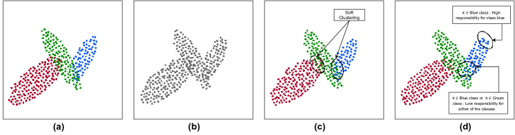
Figure 3: The categorization of hybrid Quantum Noise : (a) Original data with specific cluster; (b) Unlabeled data for finding the original clusters; (c) GMM used for soft-clustering; (d) Responsibility of a cluster.

It is important to note that (2) is the most general form of a Gaussian channel, where $\mathbf{A}$ serves the purpose of amplification, attenuation, and rotation in phase space. In contrast, the contribution $\mathbf{Z}$ is a noise term that can consist of quantum (required to make the mapped physical) and classical noise. Interestingly, ${\mathbf{A}}$ can be any real matrix. Therefore, any map $\boldsymbol{\gamma}\mapsto{\mathbf{A}^{T}}\boldsymbol{\gamma}\mathbf{A}$ can be made approximately, as long as ‘sufficient noise’ is added [8],[38]. According to (2), a single quantum link can be expressed as $\boldsymbol{\gamma}\mapsto\boldsymbol{\gamma}+\mathbf{Z}$, where $\mathbf{Z}$ indicates that the noise term consists of the quantum and the classical part. In (2), consider $\mathbf{A=I_{2x1}}$ as $\mathbf{A}$ can be any real matrix. The only condition for the map above to be a quantum channel is to ensure that sufficient noise is added [8],[38]. Therefore, ${\mathbf{A}^{T}}\mathbf{\gamma A}$ is a scalar, and the corresponding noise $Z$ added to the system can be viewed as a scalar. In terms of a mathematical equation, this unity quantum communication channel can be expressed as $Y=X+Z$, where $X$, $Y$, and $Z$ correspond to the random variables of the transmitted signal, the received signal, and the noise affecting the channel resulting from different unwanted sources, respectively.

For a realistic quantum communication network carrying classical information, it is assumed that the communication links suffer from classical and quantum noise components with the assumption that the hybrid quantum-classical noise is additive in nature, such that $Z=Z_{1}+Z_{2}$, where $Z_{1}$ is the Poisson distributed quantum shot noise and $Z_{2}$ is the Gaussian distributed white classical noise [7]. In this relation, Fig. 2 explains the theory in the schematic diagram.

II-B Hybrid Noise model

For quantum communication, it is essential to model the realistic quantum noise of a quantum channel. Previous studies show that quantum noise is widely represented as Poissonian noise [39, 40, 41]. However, a practical quantum link also suffers from noise sources that contribute non-quantum noises, such as classical noise sources [42, 43, 44, 45]. Classical noise is the integrated part of the quantum channel and must be addressed to model the realistic quantum channel. In the semi-classical theory of photodetection, the shot noise level corresponding to Poissonian photoelectron statistics is the fundamental detection limit. Hence, the shot noise power level is often called the quantum limit or the standard quantum limit of detection. For a similar reason, shot noise is often called quantum noise [46]. By considering the qubit noise as Poissonian and the classical noise as additive white Gaussian, one can expect a hybrid quantum noise represented by the following p.d.f. [7],

$$f_{Z}(z)=\sum_{i=0}^{\infty}\frac{e^{-\lambda}\lambda^{i}}{i!}\frac{1}{\sigma_{Z_{2}}\sqrt{2\pi}}e^{-\frac{1}{2}\Big{(}\frac{z-i-\mu_{Z_{2}}}{\sigma_{Z_{2}}}\Big{)}^{2}}.\\$$ (3)

II-C Quantum Transmitted Signal Model

For the transmitted signal model, let us consider a Gaussian distributed signal for the continuous-variable (CV) system. Mathematically, a state is Gaussian if its distribution function in phase or its density operator in the Fock space is Gaussian. Examples of Gaussian functions are well-known p.d.f. of Normal distribution, Wigner function, etc. Important quantum information processing experiments are done with quantum light, described as Gaussian distributed. In our model, the input quantum signal $X$ in terms of qubits is in a Gaussian state, and it can be characterized by the scalar random variable $X$ having a Gaussian distribution with parameters $\mu_{X}$ and $\sigma_{X}$, $X~{}\sim\mathcal{N}(x;\mu_{X},\,\sigma_{X}^{2})$ the p.d.f. $f_{X}$ of $X$ can be expressed as,

$$f_{X}(x)=\frac{1}{\sigma_{X}\sqrt{2\pi}}e^{-\frac{1}{2}\big{(}\frac{x-\mu_{X}}{\sigma_{X}}\big{)}^{2}}$$

where $\mu_{X}$ and $\sigma_{X}$ are the mean and standard deviation (s.d.) of the distribution.

III Methodology

In this section, we start with a brief overview of the proposed analytical framework. Beginning with the hybrid quantum noise model identified as an infinite mixture of Gaussian with weightage coming from Poisson distribution, this research aims to identify the quantum noise model with a finite number of Gaussian keeping weightage from Poisson distribution. This will help determine the clusters to visualize the quantum noise data in higher dimensions.

The ML algorithm has been used to update the parametric values of the quantum noise model; the set of parameters is the Poisson parameter, Gaussian means and variances, and their mixing coefficients. Primarily, the capacity for the signal-to-noise ratio has been plotted based on the newly updated channel parameters and compared with the existing capacity model of the quantum channel [7]. Note that the transmitted signal has been considered Gaussian for both models. Fig. 1 explains the flow of the research methodology.

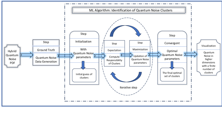
Figure 4: The process of updating channel parameters and finding optimal clusters of quantum noise using ML model

III-A Clustering with Gaussian Mixture Model

Let us start with the hybrid quantum noise model in (3),

$$\begin{split}f_{Z}(z)&=\sum_{i=0}^{\infty}w_{i}.\mathcal{N}(z;\mu_{i}^{(z)},\,{\sigma_{i}^{(z)}}^{2}),\end{split}$$ (4)

where $w_{i}=\frac{e^{-\lambda}\lambda^{i}}{i!}$ represent the weightage of the mixtures of Gaussians, $\sum_{i=0}^{\infty}w_{i}=1$, $w_{i}\geq 0\quad\forall i$ and $\mathcal{N}(z;\mu_{i}^{(z)},\,{\sigma_{i}^{(z)}}^{2})$ is the Gaussian density in random variable $Z$, mean $\mu_{i}^{(z)}=\mu_{Z_{2}}+i$ and ${\sigma_{i}^{(z)}}^{2}={\sigma_{Z_{2}}}^{2}$ with standard deviation $\sigma_{i}^{(z)}$ and variance ${\sigma_{i}^{(z)}}^{2}$. These lead to visualizing the noise model data in a scalar space or lower dimensions. In the meantime, this infinite mixture can be approximated by a finite number of components as

$$\begin{split}f_{Z}(z)=\sum_{i=0}^{R}w_{i}.\mathcal{N}\Big{(}z;\mu_{i}^{(z)},\,{\sigma_{i}^{(z)}}^{2}\Big{)}.\end{split}$$ (5)

This is the Gaussian mixture in the scalar variable $Z$, $w_{i}\geq 0\quad\forall i$ and $\sum_{i=0}^{R}w_{i}\approx 1$ for large $R$. However, a higher-dimensional approach is needed to visualize the original hybrid quantum noise data in the corresponding vector space as a scatter plot. This leads to the noise p.d.f. in a higher dimension given by the corresponding Gaussian mixture in a random vector $\mathbf{z}\in\mathbb{R}^{D}$ as

$$f_{\boldsymbol{Z}}(\mathbf{z})=\sum_{i=0}^{R}w_{i}.\mathcal{N}\Big{(}\mathbf{z};\boldsymbol{\mu}_{i}^{(z)},\,{\boldsymbol{\Sigma}_{i}^{(z)}}\Big{)},$$ (6)

where $w_{i}=\frac{e^{-\lambda}\lambda^{i}}{i!}$ represents the weightage of the Gaussian mixtures, $\mathbf{z}$ is the random vector in $\mathbb{R}^{D}$, $D$ denotes the dimension of the vector $\mathbf{z}$, $\boldsymbol{\mu}_{i}^{(z)}$ is the mean vector , $\boldsymbol{{\Sigma}}_{i}^{(z)}$ is the covariance matrix of the corresponding Gaussian density $\mathcal{N}$, and the multivariate Gaussian is given by

$$\mathcal{N}(\mathbf{z}_{n};\boldsymbol{\mu}_{k}^{(z)},\boldsymbol{\Sigma}_{k}^{(z)})\\ =\frac{1}{(2\pi)^{D/2}|\boldsymbol{\Sigma}_{k}^{(z)}|^{1/2}}e^{-\frac{1}{2}(\mathbf{z}_{n}-\boldsymbol{\mu}_{k}^{(z)})^{T}\{\boldsymbol{\Sigma}_{k}^{(z)}\}^{-1}(\mathbf{z}_{n}-\boldsymbol{\mu}_{k}^{(z)})}.$$ (7)

Consider the hybrid quantum-classical noise data set $\boldsymbol{Z}=\{\mathbf{z}_{1},\mathbf{z}_{2},...,\mathbf{z}_{n}\}$, $\mathbf{z}_{i}\in\mathbb{R}^{D}$, where $D$ denotes the dimension of the data points, respectively. The primary purpose of this research is to understand the multidimensional hybrid quantum-classical noise data set by partitioning it into $K$ number of clusters, maximizing the likelihood of the probabilistic model. The hybrid quantum noise model in (6) can be expressed as

$$f_{\boldsymbol{Z}}(\mathbf{z})=\sum_{t}f_{\boldsymbol{Z}}(\mathbf{z},t)=\sum_{t}{}f_{\boldsymbol{Z}}(\mathbf{z}|t)f_{\boldsymbol{Z}}(t),$$ (8)

where $t$ is the latent variable, which approximates the distribution with a mixture of Gaussians. To use the EM algorithm to identify the cluster of components in the hybrid quantum-classical noise data set, a discrete random variable must be introduced, which will pick the clusters (here $t$ being the $t$th component of the mixture) that satisfy the condition that the points in the cluster must be Gaussian distributed with the respective parametric value of the cluster.

The EM algorithm performs better in classifying the classical data set and is more flexible than the $K$-means algorithm for classical data. However, the limitation of this research is that we should have compared the result with the $K$-means algorithm for our hybrid quantum-classical noise data set. From (6), this research guarantees the Gaussian distribution for each latent variable $t$ conditional distribution $f_{\boldsymbol{Z}}(\mathbf{z}|t)$. In (8), $f_{\boldsymbol{Z}}(\mathbf{z}|t)$ are Gaussian p.d.f.s, and $f_{\boldsymbol{Z}}(t)$ are mixing coefficients. It is the weighting of the distribution $f_{\boldsymbol{Z}}(\mathbf{z}|t)$ with a particular probability $f_{\boldsymbol{Z}}(t)$. Together, these two quantities, the sum $\sum_{t}{}f_{\boldsymbol{Z}}(\mathbf{z}|t)f_{\boldsymbol{Z}}(t)$ represents the GMM, and $f_{\boldsymbol{Z}}(\mathbf{z}|t)$ is the posterior probabilities of the latent variable $t$ given an observable $\mathbf{z}$. That is if one observes a particular quantum data point $\mathbf{z}$, one can check the probability that it belongs to a cluster set red, green, or blue depending on the number of clusters considered case by case. For example, from the colour code model shown in Fig. 3(a), if the point comes from the blue class, it is coloured blue. If the point is in the green class, it shows the green dot. If the point belongs to the red class, it will indicate the red-coloured dot. However, the unclassified data are shown in Fig. 3(b). For the chosen data point, the uncertainty of specification of the cluster lies when these colours are mixed or overlapped, indicated with black circles in Fig. 3$(c)$, this is called “soft cluster”. According to this probabilistic model, if a data point is assigned, it is assigned the probability of belonging to one of the classes. It is not specifically inferred that it belongs to the blue class, but it is inferred that with this probability it belongs to the blue class. It is the “responsibility” that the class will take for the point to be in the class shown in Fig. 3 $(d)$. This is the setting for the GMM. It is a way to classify assignments in a soft and probabilistic way.

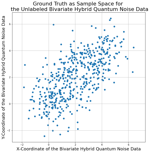
Figure 5: The ground truth data of quantum noise sampling generated as a convolution of Additive White Gaussian Noise and Poissonian quantum noise

Let us begin by considering the p.d.f. for the model as defined in (8). The p.d.f. of the GMM, which models the distribution of data points in a clustering scenario, is given by (8). The discrete latent variable $t_{k}\in\{0,1\}$ for the $K$ clusters is represented by the prior

$$f_{\boldsymbol{Z}}(t_{k}=1)=\frac{e^{-\lambda}\lambda^{k}}{k!},$$

$k\in[0,K]$, $\sum_{k=1}^{K}\frac{e^{-\lambda}\lambda^{i}}{i!}\approx 1$ for a sufficient choice of $K$. The clusters of the underlying components are Gaussians, with different parameters:

$$f_{\boldsymbol{Z}}(\mathbf{z}|t_{k}=1)=\mathcal{N}\Big{(}\mathbf{z};\boldsymbol{\mu}_{k}^{(z)},\,{\boldsymbol{\Sigma}_{k}^{(z)}}\Big{)}.$$

The quantity $t_{k}\in\{0,1\}$ indicates whether the data point $\mathbf{z}$ belongs to the $K$-th class or not. Specifically, $t_{k}=0$ means that $\mathbf{z}$ does not belong to the $K$-th class ($t_{k}\notin K$-th class), and $t_{k}=1$ means that $\mathbf{z}$ belongs to the $K$-th class ($t_{k}\in K$-th class). The probability that the data point $\mathbf{z}$ belongs to the $K$-th class is denoted by $f_{\boldsymbol{Z}}(t_{k}=1)$. Consequently, the joint probability distribution of the data point $\mathbf{z}$ and the class membership $t_{k}$ can be expressed as

$$f_{\boldsymbol{Z}}(\mathbf{z},t_{k}=1)=f_{\boldsymbol{Z}}(\mathbf{z}|t_{k}=1)f_{\boldsymbol{Z}}(t_{k}=1)$$

$$=\frac{e^{-\lambda}\lambda^{k}}{k!}\mathcal{N}\Big{(}\mathbf{z};\boldsymbol{\mu}_{k}^{(z)},\,{\boldsymbol{\Sigma}_{k}^{(z)}}\Big{)}$$

and the full generic model is given by

$$f_{\boldsymbol{Z}}(\mathbf{z};w,\boldsymbol{\mu},\boldsymbol{\Sigma})=\sum_{t}f_{\boldsymbol{Z}}(\mathbf{z},t)\\ =\sum_{k}\frac{e^{-\lambda}\lambda^{k}}{k!}\mathcal{N}\Big{(}\mathbf{z};\boldsymbol{\mu}_{k}^{(z)},\,{\boldsymbol{\Sigma}_{k}^{(z)}}\Big{)}.$$ (9)

The posterior or conditional probability of $t$ (the latent cluster) given a point $\mathbf{z}$ is

$$f_{\boldsymbol{Z}}(t_{k}=1|\mathbf{z})=\frac{f_{\boldsymbol{Z}}(t_{k}=1)f_{\boldsymbol{Z}}(\mathbf{z}|t_{k}=1)}{f_{\boldsymbol{Z}}(\mathbf{z})}\\ =\frac{f_{\boldsymbol{Z}}(t_{k}=1)f_{\boldsymbol{Z}}(\mathbf{z}|t_{k}=1)}{\sum_{j}{}f_{\boldsymbol{Z}}(t_{j}=1)f_{\boldsymbol{Z}}(\mathbf{z}|t_{j}=1)}\\ =\frac{\frac{e^{-\lambda}\lambda^{k}}{k!}\mathcal{N}\Big{(}\mathbf{z};\boldsymbol{\mu}_{k}^{(z)},\,{\boldsymbol{\Sigma}_{k}^{(z)}}\Big{)}}{\sum_{j}{}\frac{e^{-\lambda}\lambda^{j}}{j!}\mathcal{N}\Big{(}\mathbf{z};\boldsymbol{\mu}_{k}^{(z)},\,{\boldsymbol{\Sigma}_{k}^{(z)}}\Big{)}}=\gamma(z).$$

Inferring a latent cluster for an observed point $\mathbf{z}$ probabilities can be assigned to this point that belongs to one of these unobserved clusters. $f_{\boldsymbol{Z}}(t_{k}=1|\mathbf{z})=\gamma(z)$ is the formula for obtaining the conditional posterior for the observed data point $\mathbf{z}$ that belongs to one of the latent clusters. We will call $\gamma$ the responsibility that class $K$ takes to explain the data point $\mathbf{z}$.

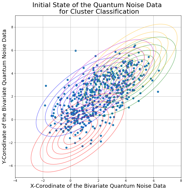
Figure 6: The initial guess of Gaussian Mixture clusters of bivariate hybrid quantum noise sample data

EM produced a set of these parametric values $w,\boldsymbol{\mu}^{(z)},\boldsymbol{\Sigma}^{(z)}$ to infer what parameters are the most optimal and which parameters lead to the distribution that most likely explains the hybrid quantum-classical noise data set. Therefore, we need to define the log-likelihood function and want to maximize it to find optimal parameters that describe the hybrid quantum-classical noise dataset.The log-likelihood of the hybrid quantum noise can be expressed as

$$\begin{split}&\ln f_{\boldsymbol{Z}}\Big{(}\mathbf{z};w,\boldsymbol{\mu}^{(z)},\,\boldsymbol{\Sigma}^{(z)}\Big{)}\\ &=\sum_{n=1}^{N}\ln\Big{(}\sum_{k=1}^{K}\frac{e^{-\lambda}\lambda^{k}}{k!}\mathcal{N}(\mathbf{z}_{n};\boldsymbol{\mu}_{k}^{(z)},\boldsymbol{\Sigma}_{k}^{(z)})\Big{)}\end{split}$$ (10)

where $N$ is referred to as the total number of hybrid quantum noise data points named sample data. To maximize the log-likelihood function, in (10), the expression cannot be further simplified due to the logarithmic summation over the total number of clusters. However, one of the solutions can be to use the ML-based EM algorithm. One needs to improve iteratively or log-likelihood using this algorithm.

III-B Maximization of log-likelihood to find optimal parametric values for classifying the clusters:

We need to maximize $\ln f_{\boldsymbol{Z}}(\mathbf{z};w,\boldsymbol{\mu}^{(z)},\boldsymbol{\Sigma}^{(z)})$ w.r.t. $\frac{e^{-\lambda}\lambda^{k}}{k!},\boldsymbol{\mu}_{k}^{(z)},\boldsymbol{\Sigma}_{k}^{(z)}$ $\forall k=1(1)K$, where $K$ is the total number of clusters. The problem is convex. Maximizing by looking for stationary points of logarithmic likelihood implies optimizing with respect to parameters $\frac{e^{-\lambda}\lambda^{k}}{k!},\boldsymbol{\mu}_{k}^{(z)},\boldsymbol{\Sigma}_{k}^{(z)}$. Therefore, we set the partial derivative of the log-likelihood function with respect to the mean vector $\boldsymbol{\mu}_{k}^{(z)}$ of the $K$-th class to zero

$$\frac{\partial}{\partial\boldsymbol{\mu}_{k}^{(z)}}\ln f_{\boldsymbol{Z}}(\mathbf{z};w,\boldsymbol{\mu}^{(z)},\boldsymbol{\Sigma}^{(z)})=0,$$ (11)

and solve it for $\boldsymbol{\mu}_{k}^{(z)}$. However, this equation does not have a closed-form solution. The stationary points depend on the posterior $\gamma(t_{n,k})$. It can find local minima using the so-called alternative update algorithm of the (expected) posterior iterative algorithm $\gamma(t_{n,k})$ and maximization for parameters $\frac{e^{-\lambda}\lambda^{k}}{k!},\boldsymbol{\mu}_{k}^{(z)},\boldsymbol{\Sigma}_{k}^{(z)}$. In (11), if we take the derivative, it depends on the parameters $\boldsymbol{\mu}_{k}^{(z)},\boldsymbol{\Sigma}_{k}^{(z)}$ and $\frac{e^{-\lambda}\lambda^{k}}{k!}$. Instead of this, we could write the solution for $\boldsymbol{\mu}_{k}^{(z)}$ as a function of responsibility $\gamma(t_{n,k})$, that is, $\frac{\partial}{\partial\boldsymbol{\mu}_{k}^{(z)}}\ln f_{\boldsymbol{Z}}(z;\frac{e^{-\lambda}\lambda^{k}}{k!},\boldsymbol{\mu}_{k}^{(z)},\mathbf{\Sigma_{k}^{(z)}})=0$ $\implies\boldsymbol{\mu}_{k}^{(z)}$ is a function of $\gamma(t_{n,k})$ and $\gamma(t_{n,k})$ depends on $\frac{e^{-\lambda}\lambda^{k}}{k!},\boldsymbol{\mu}_{k}^{(z)},\boldsymbol{\Sigma}_{k}^{(z)}$. The proposed solution is to group all remaining parameters in this term of responsibility. Therefore, the term of responsibility still depends on other parameters $\frac{e^{-\lambda}\lambda^{k}}{k!},\boldsymbol{\Sigma}_{k}^{(z)},$ even on $\mathbf{\mu_{k}}$. Using the EM algorithm, to fix the posterior probability or the responsibility $\gamma(t_{n,k})$ and solve for the case $\boldsymbol{\mu}_{k}^{(z)}$ and all the other parameters, one can update the responsibilities and again iterate this solution for maximization and solve for the parameters.

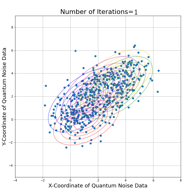
Figure 7: 1st iteration result under the updating of component of Gaussian Mixture clusters of the bivariate hybrid quantum noise sample data

Lemma 1.

The maximizing log-likelihood in (10) w.r.t. $\boldsymbol{\mu}_{k}^{(z)}$ by setting derivative of the log-likelihood w.r.t. $\boldsymbol{\mu}_{k}^{(z)}$ to $0$

$$\frac{\partial}{\partial\boldsymbol{\mu}_{k}^{(z)}}\ln f_{\boldsymbol{Z}}(\mathbf{z};w,\boldsymbol{\mu}^{(z)},\mathbf{\Sigma^{(z)}})=0,$$

gives

$$\boldsymbol{\mu}_{k}^{(z)}=\frac{\sum_{n=1}^{N}\gamma(t_{n,k})\mathbf{z}_{n}}{\sum_{n=1}^{N}\gamma(t_{n,k})}$$

Proof:

Please refer to Appendix A. ∎

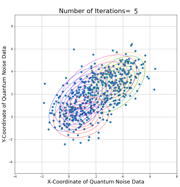
Figure 8: The result after iteration size 5 for the updating of component of Gaussian Mixture clusters of the bivariate hybrid quantum noise sample data

Now, to maximize the log-likelihood with respect to the mixing coefficient, $\ \frac{e^{-\lambda}\lambda^{k}}{k!}$ by considering a constrained optimization problem using the Lagrange multiplier method. To maximize log-likelihood w.r.t. $\frac{e^{-\lambda}\lambda^{k}}{k!}$ we have to set the derivative of the log-likelihood w.r.t. $\frac{e^{-\lambda}\lambda^{k}}{k!}$ to $0$, under the constraint that the sum of the probabilities $\sum_{k=1}^{K}\frac{e^{-\lambda}\lambda^{k}}{k!}$, add up to one, that is, $\sum_{k=1}^{K}\frac{e^{-\lambda}\lambda^{k}}{k!}=1$.

Let the Lagrange multipliers be denoted by

$$L(\frac{e^{-\lambda}\lambda^{k}}{k!},\Lambda):=f(\mathbf{z}_{n})+\Lambda(g(\mathbf{z}_{n})-c)$$

where $f(\mathbf{z}_{n})=\sum_{n=1}^{N}\ln f_{\boldsymbol{Z}}(\mathbf{z}_{n};\frac{e^{-\lambda}\lambda^{k}}{k!},\boldsymbol{\mu}_{k}^{(z)},\boldsymbol{\Sigma}_{k}^{(z)})$ , $g(\mathbf{z}_{n})=\sum_{k=1}^{K}\frac{e^{-\lambda}\lambda^{k}}{k!}$ and $c=1$. Let us set the partial derivative of the Lagrange multipliers w.r.t. $\frac{e^{-\lambda}\lambda^{k}}{k!}$ that is $\frac{\partial}{\partial w_{k}}L(w,\Lambda)=0$ gives

$$\frac{\partial}{\partial\frac{e^{-\lambda}\lambda^{k}}{k!}}\Bigg{[}\sum_{n=1}^{N}\ln f_{\boldsymbol{Z}}(\mathbf{z}_{n};w,\boldsymbol{\mu},\boldsymbol{\Sigma})\\ +\Lambda\bigg{\{}\sum_{k=1}^{K}\frac{e^{-\lambda}\lambda^{k}}{k!}-1\bigg{\}}\Bigg{]}=0\\ \implies\sum_{n=1}^{N}\frac{1}{f_{\boldsymbol{Z}}(\mathbf{z}_{n};w,\boldsymbol{\mu},\boldsymbol{\Sigma})}\frac{\partial}{\partial\frac{e^{-\lambda}\lambda^{k}}{k!}}f_{\boldsymbol{Z}}(\mathbf{z}_{n};w,\boldsymbol{\mu},\boldsymbol{\Sigma})\\ +\Lambda\frac{\partial}{\partial\frac{e^{-\lambda}\lambda^{k}}{k!}}\bigg{\{}\sum_{k=1}^{K}\frac{e^{-\lambda}\lambda^{k}}{k!}-1\bigg{\}}=0$$ (12)

$$\implies\sum_{n=1}^{N}\frac{\frac{\partial}{\partial\frac{e^{-\lambda}\lambda^{k}}{k!}}\Big{[}\sum_{k=1}^{K}\frac{e^{-\lambda}\lambda^{k}}{k!}\mathcal{N}(\mathbf{z}_{n};\boldsymbol{\mu}_{k}^{(z)},\boldsymbol{\Sigma}_{k}^{(z)})\Big{]}}{\sum_{k=1}^{K}\frac{e^{-\lambda}\lambda^{k}}{k!}\mathcal{N}(\mathbf{z}_{n};\boldsymbol{\mu}_{k}^{(z)},\boldsymbol{\Sigma}_{k}^{(z)})}$$

$$+\Lambda\frac{\partial}{\partial\frac{e^{-\lambda}\lambda^{k}}{k!}}\bigg{\{}\sum_{k=1}^{K}\frac{e^{-\lambda}\lambda^{k}}{k!}-1\bigg{\}}=0$$

$$\implies\frac{e^{-\lambda}\lambda^{k}}{k!}=-\frac{1}{\Lambda}\sum_{n=1}^{N}\gamma(t_{n,k}).$$

Now solve it for $\Lambda$. For that, we consider the constraint part $\sum_{k=1}^{K}\frac{e^{-\lambda}\lambda^{k}}{k!}=1.$. Now, setting derivative of the Lagrange multipliers w.r.t. $\Lambda$ to zero ,that is $\frac{\partial}{\partial\Lambda}L(\frac{e^{-\lambda}\lambda^{k}}{k!},\Lambda)=0\implies\frac{\partial}{\partial\Lambda}\big{\{}f(\mathbf{z}_{n})+\Lambda(g(\mathbf{z}_{n})-c)\big{\}}=0\implies\sum_{k=1}^{K}\frac{e^{-\lambda}\lambda^{k}}{k!}-1=0\\ \implies-\frac{1}{\Lambda}\sum_{n=1}^{N}\sum_{k=1}^{K}\gamma(t_{n,k})=1\implies\Lambda=-N$, because $\sum_{k=1}^{K}\gamma(t_{n,k})=\sum_{k=1}^{K}f_{\boldsymbol{Z}}(t_{n,k}|\mathbf{z})=1$, this is due to the sum of all classes. Finally, this gives us

$$w_{k}=\frac{1}{N}\sum_{n=1}^{N}\gamma(t_{n,k}).$$

Now we need to calculate the expression for $\boldsymbol{\Sigma}_{k}^{(z)}$.

Lemma 2.

The maximization of the log-likelihood in (10) w.r.t. $\boldsymbol{\Sigma}_{k}^{(z)}$ by setting

$$\frac{\partial}{\partial\boldsymbol{\Sigma}_{k}^{(z)}}\ln f_{\boldsymbol{Z}}(\mathbf{z};w,\boldsymbol{\mu},\boldsymbol{\Sigma})=0,$$

gives

$$\boldsymbol{\Sigma}_{k}^{(z)}=\frac{\sum_{n=1}^{N}\gamma(t_{n,k})(\mathbf{z}_{n}-\mu_{k}^{(z)})(\mathbf{z}_{n}-\mu_{k}^{(z)})^{T}}{\sum_{i=1}^{N}\gamma(t_{n,k})}.$$

Proof:

Please refer to Appendix B. ∎

Now define the effective number of points in cluster K by

$$N_{k}=\sum_{n=1}^{N}\gamma(t_{n,k}).$$

Hence, the solution for $\frac{e^{-\lambda}\lambda^{k}}{k!},\mu_{k}^{(z)},\boldsymbol{\Sigma}_{k}^{(z)}$ (dependent on the posterior) can be written as

$$\begin{split}&\boldsymbol{\mu}_{k}^{(z)}=\frac{1}{N_{k}}\sum_{n=1}^{N}\gamma(t_{n,k})\mathbf{z}_{n},\\ &\frac{e^{-\lambda}\lambda^{k}}{k!}=\frac{N_{k}}{N},\\ &\boldsymbol{\Sigma}_{k}^{(z)}=\frac{1}{N_{k}}\sum_{n=1}^{N}\gamma(t_{n,k})(\mathbf{z}_{n}-\boldsymbol{\mu}_{k}^{(z)})(\mathbf{z}_{n}-\boldsymbol{\mu}_{k}^{(z)})^{T}.\\ \end{split}$$ (13)

III-C Expectation-Maximization Algorithm (EM):

The EM algorithm is a robust technique for estimating parameters in GMMs. This iterative algorithm comprises two primary steps: the expectation step (E step) and the maximization step (M step). Initially, the GMM parameters are established, which involve initialization of the means $\boldsymbol{\mu}_{k}^{(z)}$, covariances $\boldsymbol{\Sigma}_{k}^{(z)}$, and the probabilities of the mixture component expressed as $\frac{e^{-\lambda}\lambda^{k}}{k!}$ for each component $k$. In step E, the algorithm updates the expected posterior probabilities, or responsibilities $\gamma(z_{n,k})$, for each data point that concerns each component of the mixture. This step estimates the degree to which each component generates each data point. Subsequently, the M step aims to maximize the log-likelihood of the model given the current parameter estimates, adjusting $\boldsymbol{\mu}_{k}^{(z)}$, $\boldsymbol{\Sigma}_{k}^{(z)}$, and the probabilities based on the fixed posteriors established in the E step. The algorithm alternates between these E and M steps until it meets a convergence criterion, such as a negligible change in the log-likelihood or after a specified number of iterations. This iterative process allows the EM algorithm to efficiently find local minima in the optimization landscape of the GMM parameter estimation problem.

1

2

3

Input: $\lambda$, $\boldsymbol{\mu}_{k,0}^{(z)}$, $\boldsymbol{\Sigma}_{k,0}^{(z)}$, $k=1(1)K$

4

Output: $\boldsymbol{\mu}_{k,m}^{(z)}$, $\boldsymbol{\Sigma}_{k,m}^{(z)}$

5

6$m\leftarrow 1$

7repeat

8      

9      ​​ Calculate the responsibilities $\gamma(z_{n,k,m})$ for each data point $\mathbf{z}_{n}$ and each component $k$ according to $\gamma(z_{n,k})=\frac{\frac{e^{-\lambda}\lambda^{k}}{k!}\mathcal{N}(\mathbf{z}_{n};\boldsymbol{\mu}_{k}^{(z)},\boldsymbol{\Sigma}_{k}^{(z)})}{\sum_{k=1}^{K}\frac{e^{-\lambda}\lambda^{k}}{k!}\mathcal{N}(\mathbf{z}_{n};\boldsymbol{\mu}_{k}^{(z)},\boldsymbol{\Sigma}_{k}^{(z)})}$;

10      

11      ​​ $w_{k,m}=\frac{e^{-\lambda}\lambda^{k}}{k!}=\frac{1}{N}\sum_{n=1}^{N}\gamma(\mathbf{z}_{n,k,m})$;

12      

13      ​​ $\boldsymbol{\mu}_{k,m}^{(z)}=\frac{1}{N_{k}}\sum_{n=1}^{N}\gamma(\mathbf{z}_{n,k,m})\mathbf{z}_{n}$ ;

14      

15      ​​ $\boldsymbol{\Sigma}_{k,m}^{(z)}=\frac{1}{N_{k}}\sum_{n=1}^{N}\gamma(\mathbf{z}_{n,k,m})(\mathbf{z}_{n}-\boldsymbol{\mu}_{k}^{(z)})(\mathbf{z}_{n}-\boldsymbol{\mu}_{k,m}^{(z)})^{T}$;

16      

17      $m\leftarrow m+1$;

18      

19until convergence ;

Algorithm 1 Expectation Maximization Algorithm for finding the optimal $\frac{e^{-\lambda}\lambda^{k}}{k!}$, $\boldsymbol{\mu}_{k}^{(z)}$, $\boldsymbol{\Sigma}_{k}^{(z)}$

In our probabilistic framework, which models responsibility-classical noise as a combination of several Gaussian distribution functions, as detailed in Equation (6), we outline the EM algorithm within Algorithm 1.

III-D The convergent of EM algorithm in the context of log-likelihood function

Convergence of the EM algorithm is typically understood in terms of the log-likelihood function of the observed data. In terms of monotonicity, the EM algorithm ensures that the log-likelihood function of the observed data does not decrease with each iteration [47]. Under general conditions, the EM algorithm converges to a local maximum (or saddle point in some cases) of the log-likelihood function. The convergence rate is typically linear but can slow near the maximum. The specific convergence rate can depend on the proximity of the initial parameter estimates to the actual values and the shape of the log-likelihood surface [48]. The convergence of the EM algorithm is guaranteed under certain regularity conditions, including certain derivatives of the log-likelihood function and the boundedness of the parameter space. However, these conditions can sometimes only be strictly met in practice, leading to convergence to local optima or, in rare cases, divergence if assumptions are violated severely [49].

For practical considerations, the EM algorithm’s convergence is usually monitored by checking the change in the log-likelihood value or the change in parameter estimates between successive iterations. Convergence is assumed when these changes fall below a predetermined threshold. It is also common to set a maximum number of iterations to prevent infinite looping in cases where convergence is slow or the algorithm oscillates.

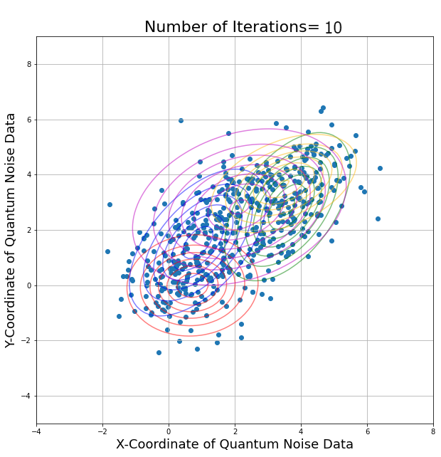
Figure 9: The result after iteration size 10 for the updating of component of Gaussian Mixture clusters of the bivariate hybrid quantum noise sample data.

III-E Discusssion on selecting GMM in comparison to existing ML models

GMM stands out among other ML models due to its flexibility, probabilistic foundation, and ability to model complex distributions. First, its flexibility in modeling distributions allows it to approximate almost any continuous density function, making it ideal for datasets with multiple subpopulations or clusters. Unlike single-Gaussian models, GMMs can effectively capture diverse data structures [26]. Second, GMM offers soft clustering, assigning to each data point a probability of belonging to each cluster, enabling nuanced grouping and analysis [50]. This contrasts with hard clustering methods like K-means. Third, GMM’s probabilistic framework inherently accommodates uncertainty in data, ensuring robust modeling results in noisy or incomplete datasets [51]. Lastly, GMM facilitates parameter estimation via the Expectation-Maximization (EM) algorithm, iteratively refining data likelihood under the model. Additionally, model selection criteria such as Bayesian or Akaike Information Criterion are directly applicable to GMMs, helping to determine the optimal number of components [52][53].

IV Application in Maximization of Quantum Channel Capacity

In quantum channel modeling, the interplay between the Poisson parameter and the GMM is fundamental to accurately simulating quantum noise. The Poisson parameter, $\lambda$, quantifies the average photon count detected over a specific interval, highlighting the quantum nature of light and the stochastic process of photon emission and detection. This parameter is essential for modeling photon statistics in quantum optics [40, 39], where photon arrivals at a detector are typically Poisson distributed, reflecting the quantized nature of light. On the contrary, the GMM provides a probabilistic framework for modeling quantum noise, encompassing both quantum and classical noise influences on quantum states during transmission [53]. This allows for a more comprehensive representation of various noise sources and their statistical behaviors in a quantum channel. The connection between these two models lies in their joint capability to more accurately represent the complexity of quantum noise [54]. Although the Poisson parameter $\lambda$ captures the quantum mechanical aspects of the photon distribution, the GMM accounts for a broader range of noise scenarios, including classical noise effects such as thermal noise and detector inefficiencies [38]. This blend facilitates nuanced understanding and optimization of quantum channels, enabling the development of sophisticated error correction codes and communication protocols tailored to mitigate the specific noise characteristics encountered in quantum information transfer.

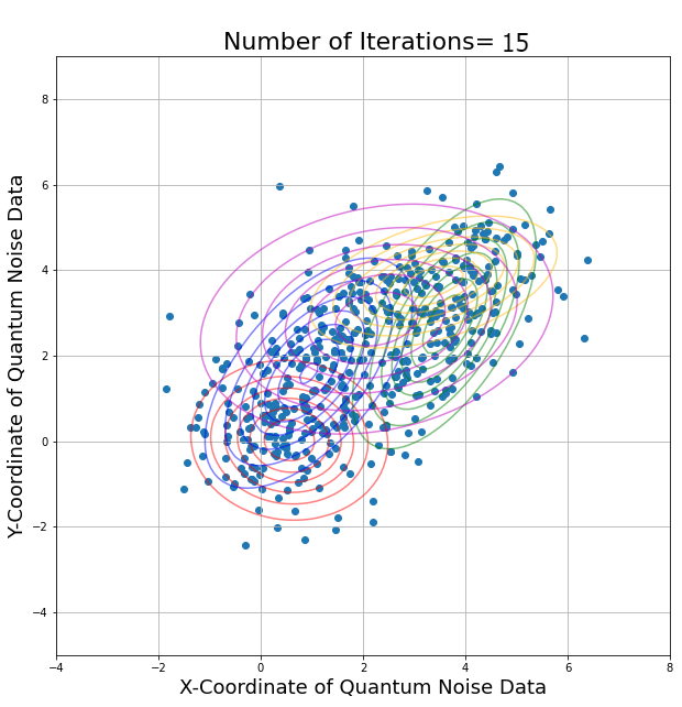
Figure 10: The result after iteration size 15 under the updating of component of Gaussian Mixture clusters of the bivariate hybrid quantum noise sample data.

Taking into account hybrid quantum noise and the Gaussian transmitted signal model as discussed above [7], the capacity of the quantum channel can be expressed as follows:
$C=\sum_{i=0}^{R}\frac{e^{-\lambda}\lambda^{i}}{i!}\Bigg{(}-\log_{2}\Big{(}\frac{e^{-\lambda}\lambda^{i}}{i!}\Big{)}+\frac{1}{2}\log_{2}{\Big{(}(2\pi e)^{M}\big{|}{\boldsymbol{\Sigma}}_{i}^{(y)}\big{|}\Big{)}}\\ +\log_{2}\Big{(}\sum_{j=0}^{R}\frac{e^{-\lambda}\lambda^{j}}{j!}\mathcal{N}\Big{(}\boldsymbol{\mu}_{i}^{(z)};\boldsymbol{\mu}_{j}^{(z)},\,{\boldsymbol{\Sigma}}_{i}^{(z)}+{\boldsymbol{\Sigma}}_{j}^{(z)}\Big{)}\Big{)}\Bigg{)}$.

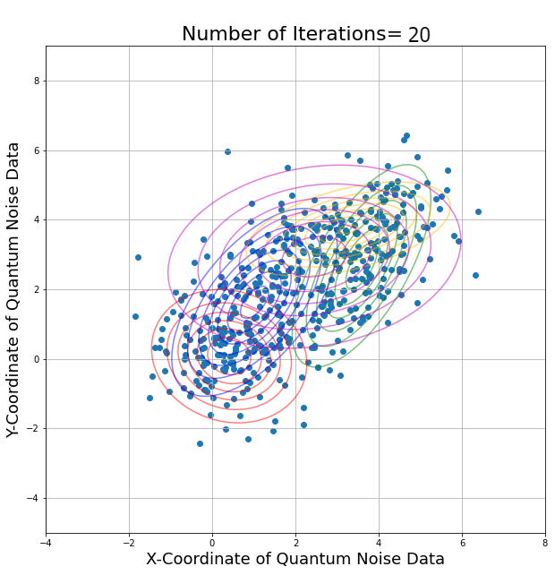
Figure 11: The Final results corresponding to iteration size 20 under the updating of component of Gaussian Mixture clusters of the bivariate hybrid quantum noise sample data.

This formula delineates the capacity of the quantum channel for scenarios where both the noise $\boldsymbol{Z}$ and the received signal $\boldsymbol{Y}$ are represented as random vectors of dimension size $M$. In scalar analogy, that is, when the noise $Z$ with scalar p.d.f., the expression of capacity reduces to $C=\sum_{i=0}^{R}\frac{e^{-\lambda}\lambda^{i}}{i!}\Bigg{[}-\log_{2}\Big{(}\frac{e^{-\lambda}\lambda^{i}}{i!}\Big{)}+\frac{1}{2}\log_{2}{\Big{(}2\pi e{\sigma}_{i}^{(y)}\Big{)}}+\log_{2}\Bigg{(}\sum_{j=0}^{R}\frac{e^{-\lambda}\lambda^{j}}{j!}\mathcal{N}\Big{(}{\mu_{i}}^{(z)};{\mu_{j}}^{(z)},\,{{\sigma}_{i}^{(z)}}^{2}+{{\sigma}_{j}^{(z)}}^{2}\Big{)}\Bigg{)}\Bigg{]}$,
by putting $M=1$, and replacing $\big{|}{\boldsymbol{\Sigma}}_{i}^{(y)}\big{|}$ by ${\sigma}_{i}^{(y)}$, $\boldsymbol{\mu}_{i}^{(z)}$ by $\mu_{i}^{(z)}$, $\boldsymbol{\mu}_{j}^{(z)}$ by $\mu_{j}^{(z)}$, ${\boldsymbol{\Sigma}}_{i}^{(z)}$ by ${{\sigma}_{i}^{(z)}}^{2}$ and $\boldsymbol{\Sigma}_{j}^{(z)}$ by ${{\sigma}_{j}^{(z)}}^{2}$, where each vector is replaced by its scalar analogue [7]. Again $\mu_{i}^{(z)}=\mu_{Z_{2}}+i$ $\forall i$, ${{\sigma}_{i}^{(z)}}^{2}={\sigma_{Z_{2}}}^{2}$ $\forall i$, and ${{\sigma}_{i}^{(y)}}^{2}={\sigma_{X}}^{2}+{\sigma_{Z_{2}}}^{2}$ $\forall i$. Therefore, the capacity of the quantum channel is given by

$$\begin{split}C&=\sum_{i=0}^{R}\frac{e^{-\lambda}\lambda^{i}}{i!}\Bigg{[}-\log_{2}\Big{(}\frac{e^{-\lambda}\lambda^{i}}{i!}\Big{)}\\ &+\frac{1}{2}\log_{2}{\Big{(}2\pi e\big{(}{\sigma_{X}}^{2}+{\sigma_{Z_{2}}}^{2}\big{)}\Big{)}}\\ &+\log_{2}\Bigg{(}\sum_{j=0}^{R}\frac{e^{-\lambda}\lambda^{j}}{j!}\frac{1}{\sqrt{2}\sigma_{Z_{2}}\sqrt{2\pi}}e^{-\frac{1}{2}\Big{(}\frac{i-j}{\sqrt{2}\sigma_{Z_{2}}}\Big{)}^{2}}\Bigg{)}\Bigg{]}.\end{split}$$ (14)

The updated channel parameters will be used to plot the new capacity graph with the signal-to-noise ratio using the EM algorithm. Based on the initial guess of the channel parameters, they will be compared with the capacity graph with the signal-to-noise ratio.

V Numerical Analysis

V-A Hybrid quantum noise data visualization

In this subsection, we visualize the original underlying hybrid quantum-classical noise data set in the vector field and investigate its properties. Consider our hybrid quantum-classical noise model given by (6), is a GMM consisting of a finite number of mixtures in Gaussians with a set of mixing coefficients. The weightage (coefficient) will decide the contributions of the Gaussian component, which has probability properties, explicitly represented by the prior $f_{\boldsymbol{Z}}(t_{k}=1)=\frac{e^{-\lambda}\lambda^{k}}{k!},$ $k\in[0,K],\frac{e^{-\lambda}\lambda^{k}}{k!}\in[0,1],\sum_{k=1}^{K}\frac{e^{-\lambda}\lambda^{k}}{k!}\approx 1$ where $t_{k}\in\{0,1\}$ is the discrete latent variable for the $K$ clusters. In our model, the weightage comes from the Poisson distribution, so it is necessary to carefully choose the values of these parameters for the initial guess so that the initial condition $\sum_{k=1}^{K}\frac{e^{-\lambda}\lambda^{k}}{k!}\approx 1$ will satisfy up to a specifically defined accuracy, and not only that these values will depend on the chosen value of $\lambda$. The higher value of $\lambda$ will be responsible for the more significant number of components (value of $K$). Since we intend to reduce the number of the mixture for simplicity of visualization, choose the value of $\lambda$ as low as possible. The physical interpretation of the lower value of $\lambda$ is the controlled photon emission per second.

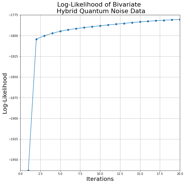
Figure 12: The log-likelihood of the bivariate hybrid quantum noise probability density function. The saturation of the curve implies the convergent of the EM algorithm for the cluster finding.

For example, set first the accuracy of $\sum_{k=1}^{K}\frac{e^{-\lambda}\lambda^{k}}{k!}\approx 1$ to be at least $85\%$, that is, $\sum_{k=1}^{K}\frac{e^{-\lambda}\lambda^{k}}{k!}>0.85$. Now, if one sets $\lambda=2$, the initial guess of the mixing coefficients can be $0.271,0.271,0.135,0.180,0.009$ (as these are the most probable values in the Poisson distribution with $\lambda=2$), the sum of these values $5$ gives $0.947$ ($>0.85$) which means that the number of clusters (that is, the value of $K$) can be considered as $5$. In another example, let $\lambda=5$, the initial guess of the mixing coefficients can be $0.175,0.175,0.146,0.140,0.104,0.084,0.065$ (since these are the most probable values in the Poisson distribution with $\lambda=5$), the sum of these values of $7$ gives $0.889$ ($>0.85$) which means that the number of clusters ( that is, the value of $K$) can be considered as $7$. However, suppose that we consider the five highest probable values $0.175,0.175,0.146,0.140,0.104$ from the Poisson distribution with $\lambda=5$ to keep the number of clusters as $K=5$. In that case, we will get the sum of $0.74<0.85$, which does not satisfy the initial condition.

Higher values of $\lambda$ will give a flatter Poisson distribution and a lower value of the mixing coefficient or weightage $w_{i}$, leading to more components in the Gaussian mixture. However, it aims to reduce the number of components in the mixture to visualize the classified clusters in the modeling quantum data. This will simplify our understanding of the underlying hybrid quantum-classical noise model. As the constraint $\sum_{i=0}^{R}w_{i}\approx 1$ for large $R$ to be satisfied up to a specific error tolerance, we set an accuracy level of $85\%$ by setting $|1-\sum_{i=0}^{R}w_{i}|\leq 0.15$, that is, we tolerate the error $15\%$. We should have a precision of at least $85\%$ while keeping the optimal number of clusters to visualize the hybrid quantum-classical noise data set.

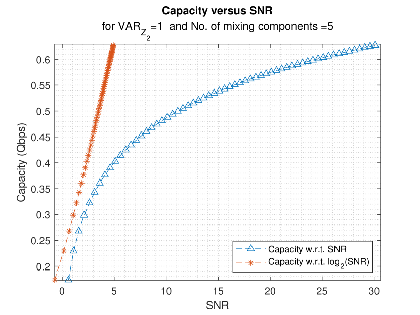
Figure 13: The capacity of the quantum channel with respect to SNR for the number of components $5$ and variance of $\sigma_{Z_{2}}^{1}=1$.

In quantum cryptography, Alice’s light source is crucial for generating the photons dispatched to Bob. It has been assumed throughout that Alice transmits photons singly to Bob. Transmitting multiple photons per pulse could inadvertently benefit Eve, the eavesdropper, by providing additional information. The issue is exacerbated with each additional photon per pulse. For instance, Eve’s chances of accurately determining the basis and bit value for many pulses with three photons per pulse increase significantly. Thus, ensuring that each light pulse contains only a single photon is paramount, though challenging in practice. The conventional approach involves using a pulsed laser and substantially attenuating its output to achieve a low mean number of photons per pulse, $\lambda$. A laser light of a single frequency exhibits Poissonian photon statistics. With a small $\lambda$, most pulses will be photon-free, a minority will have one photon, and an even smaller fraction will contain multiple photons. For example, selecting $\lambda=0.1$ is common in current quantum cryptography but results in a concerning scenario in which $5\%$ of the pulses contain more than one photon for every pulse with exactly one photon [46].

Let us visualize the model with $\lambda=2$. Our first objective is to find the optimal number of clusters $K$ with at least $85\%$ accuracy, and this is the most probable value for $\frac{e^{-\lambda}\lambda^{k}}{k!}$ from the Poisson distribution with parameter $\lambda=2$. For the initial guess of the mixing coefficient $\frac{e^{-\lambda}\lambda^{i}}{i!}\forall i=0,1,2,3,4$, choose $w_{1}=0.135$, $w_{2}=0.271$, $w_{3}=0.271$, $w_{4}=0.18$, and $w_{1}=0.09$. Now, if the condition $|1-\sum_{i=0}^{R}w_{i}|\leq 0.15$ is satisfied, it can proceed with the values and obtain the acceptable number of clusters. If the condition does not satisfy, try different values of the Poisson distribution with parameter $\lambda=2$. So, let us calculate $|1-\sum_{i=0}^{R}w_{i}|=1-(0.135+0.271+0.271+0.18+0.09)=1-0.94735=0.05265<0.15$, that is, our accuracy is $\approx 95\%$, and we tolerate the error $\approx 5\%$ allowed by our limitation limit. This will give us the optimal number of clusters $K$, $5$ within the error tolerance. Therefore, we rewrite our noise probability density function in five Gaussian mixtures,

$$f_{\boldsymbol{Z}}(\mathbf{z})=\sum_{k=0}^{K}w_{k}.\mathcal{N}\Big{(}\mathbf{z};\boldsymbol{\mu}_{k}^{(z)},\,\boldsymbol{\Sigma}_{k}^{(z)}\Big{)}$$

Figure 14: The capacity of the quantum channel with respect to SNR for the number of components $5$ and variance $\sigma_{Z_{2}}^{2}=0.687$.

We aim to find the optimal parametric values for $\boldsymbol{\mu}_{k}^{(z)}$ and $\boldsymbol{\Sigma}_{k}^{(z)}$ for $k=0,1,2,3,4$. Note that a general Gaussian mixture of five components needs an initial guess of the parameter value $15$, and at the end of the result optimal values should be obtained for these parameters $15$. However, we have fewer degrees of freedom in choosing the parametric values discussed below.

This program simulation was run in an Anaconda3 Jupyter notebook with Python to find the final values of the parameters, and this led to the classification of the clusters and visualization of the components of the hybrid-quantum classical data set. Since our number of mixing components, a.k.a. the number of clusters, is $5$, we start with the initial guess or the $\boldsymbol{\mu}_{0},\boldsymbol{\mu}_{1},\boldsymbol{\mu}_{2},\boldsymbol{\mu}_{3},\boldsymbol{\mu}_{4}$, and $\boldsymbol{\Sigma}_{0},\boldsymbol{\Sigma}_{1},\boldsymbol{\Sigma}_{2},\boldsymbol{\Sigma}_{3},\boldsymbol{\Sigma}_{4}$. In the hybrid quantum-classical noise model (6), we calculated the mean vector $\boldsymbol{\mu}_{k}^{(z)}=(\mu_{Z_{2}}+k)\mathbf{I}_{2x1}$, and covariance matrix as $\boldsymbol{\Sigma}_{k}^{(z)}=\sigma_{Z_{2}}^{2}\mathbf{I}_{2x2}$ for $k=0,1,2,3,4$. Here, $\mathbf{I}$ represents the identity matrix of the corresponding dimensions. So, start with the initial choice for mean $\mu_{Z_{2}}=0$, and variance $\sigma_{Z_{2}}^{2}=1$. Let us visualize the hybrid quantum-classical noise data set by plotting $\mathcal{N}(\mathbf{z};\boldsymbol{\mu}_{k}^{(z)},\,{\boldsymbol{\Sigma}}_{k}^{(z)})$ for $k=0,1,2,3,4$ given by Fig. 5. This unlabeled quantum noise data set will be the ground truth for the EM algorithm to find the clusters.

In the process of setting the initial estimate for the Gaussian parameters, let us start with $\boldsymbol{\mu}_{0}=\mu_{Z_{2}}\mathbf{I}_{2x1}=\mathbf{0}_{2x1},\boldsymbol{\Sigma}_{0}=\sigma_{Z_{2}}^{2}\mathbf{I}_{2x2}=\mathbf{I}_{2x2}$, based on the values chosen above of mean $\mu_{Z_{2}}$ and variance $\sigma_{Z_{2}}^{2}$. Consider the precalculated initial estimate for the mixing coefficients, which is Poisson distributed: $w_{0}=0.135$, $w_{1}=0.271$, $w_{2}=0.271$, $w_{3}=0.18$, and $w_{4}=0.09$. Fig. 6 shows the estimated clusters to choose the parametric values above for the initial guess. The following figures show how the iteration of intermediate steps iteratively updates the parametric values; the corresponding plots for the estimated clusters are shown accordingly in Fig. 7, Fig. 8, Fig. 9, Fig. 10, and Fig. 11. In particular, Fig. 11 shows the optimal clusters resulting from the EM algorithm. Fig. 12 shows the logarithmic likelihood of the density function of the hybrid quantum noise; the saturation of the function confirms the convergence of the EM algorithm, which implies that we obtained the final optimal set of the cluster for the quantum noise data set. Also, from Fig. 10 and Fig. 11, we can infer that the system model is convergent since updating does not change the clusters.

We started with the initial estimate for the parametric values $w_{0}=0.135$, $w_{1}=0.271$, $w_{2}=0.271$, $w_{3}=0.18$, $w_{4}=0.09$, and $\boldsymbol{\mu}_{0}=\mathbf{0}_{2X1}$, and $\boldsymbol{\Sigma}_{0}=\mathbf{I}_{2X2}$. We plotted the figures for the cases where the number of iterations =$1,5,10,15,20$ is shown in Fig. 7, Fig. 8, Fig. 9, Fig. 10, and Fig. 11 respectively. Finally, we get optimal values for the parameters as follows:

$$w_{0}^{\prime}=0.1871,w_{1}^{\prime}=0.3321,w_{2}^{\prime}=0.2916,$$

$$w_{3}^{\prime}=0.1487,w_{4}^{\prime}=0.0403,$$

and

$\boldsymbol{\mu}_{0}^{\prime}=\begin{bmatrix}0.4180\\ 0.0895\end{bmatrix},$ $\boldsymbol{\Sigma}_{0}^{\prime}=\begin{bmatrix}0.8910&-0.1011\\ -0.1011&0.9452\end{bmatrix}$.

From the algorithm, the optimal value is obtained as $w_{0}^{\prime}=0.1871$, this $\implies\frac{e^{-\lambda}\lambda^{0}}{0!}=0.1871$, $\implies\lambda=1.6757\approx 2$ in integer values. Therefore, as a verification, this application of the EM algorithm for finding the optimal cluster in the classification of bivariate hybrid-quantum data can update the optimal parametric values of Gaussian components and helps to identify the optimal clusters but does not affect the Poissonian parameter $\lambda$, which is the number of photon counts in the system.

However, the iterative EM algorithm has successfully updated the other two channel parameters. We will use the updated parameters to compare the quantum channel capacity for the Gaussian transmitted signal.

V-B Capacity comparison based on updated channel parameters and initial guess of parameters

Consider the expression of quantum channel capacity in (14) involving the channel parameter $\sigma_{Z_{2}}$ only to reflect any change in capacity, as we have shown that there is no change in the value of $\lambda$, and $\mu_{Z_{2}}$ does not involve the expression.

So, start with the initial value of $\boldsymbol{\Sigma}_{0}=\sigma_{Z_{2}}^{2}\mathbf{I}_{2x2}$ where $\sigma_{Z_{2}}=1$ $\longleftrightarrow$ $|\boldsymbol{\Sigma}_{0}|=1$, and updated value of $\boldsymbol{\Sigma}_{0}^{\prime}$ $\implies|\boldsymbol{\Sigma}_{0}^{\prime}|=0.829\longleftrightarrow\sigma_{Z_{2}}=0.829\implies\sigma_{Z_{2}}^{2}=0.687$.

This implies that the EM algorithm will lower the Gaussian noise variance by optimal clustering. Now, let us compare the capacity with respect to the signal-to-noise ratio (SNR) when $\sigma_{Z_{2}}^{2}=1$ and $0.687$ based on the cluster size $5$. In Fig. 13, we have plotted the benchmark result as the capacity of the quantum channel with respect to SNR for the number of components $5$ and the variance of Gaussian noise, $\sigma_{Z_{2}}^{2}=1$. Fig. 14 we plot the capacity of the quantum channel with respect to the signal-to-noise ratio for the number of components $5$ and the variance $\sigma_{Z_{2}}^{2}=0.687$. Fig. 14 gives a better result in capacity estimation compared to Fig. 13.

VI Conclusion

This work enhances quantum communication through ML, focusing on a hybrid quantum noise model that combines quantum Poissonian noise with classical white Gaussian noise. Traditionally visualized in lower dimensions, this noise has been reinterpreted as a finite GMM, with a Poisson distribution determining mixing weights. The goal was to simplify the model for easier visualization without compromising the accuracy of the original noise distribution. Using the EM algorithm, we update the channel parameters and identify optimal clusters, allowing a more precise representation of quantum noise in higher dimensions. When the capacities of the quantum channels were compared under initial and updated parameters in varying signal-to-noise ratios, it was demonstrated that ML significantly improves the accuracy of the parameters. This approach offers a more intuitive understanding of quantum noise and aids in the precise identification of noise clusters, marking a substantial advancement in the field.

Appendix

VI-A Proof of Lemma 1

The aim is to compute an expression for $\boldsymbol{\mu}_{k}^{(z)}$ as a function of responsibility $\gamma$, this can be done by setting a partial derivative of log-likelihood w.r.t. $\boldsymbol{\mu}_{k}^{(z)}$ as zero , given by $\frac{\partial}{\partial\boldsymbol{\mu}_{k}^{(z)}}\ln f_{\boldsymbol{Z}}(\mathbf{z};w,\boldsymbol{\mu}^{(z)},\mathbf{\Sigma^{(z)}})=0$

$$\implies\frac{\partial}{\partial\boldsymbol{\mu}_{k}^{(z)}}\sum_{n=1}^{N}\ln f_{\boldsymbol{Z}}(\mathbf{z}_{n};w,\boldsymbol{\mu}^{(z)},\boldsymbol{\Sigma}^{(z)})=0\\ \implies\sum_{n=1}^{N}\frac{\frac{e^{-\lambda}\lambda^{k}}{k!}\frac{\partial}{\partial\mu_{k}^{(z)}}\{\mathcal{N}\big{(}\mathbf{z}_{n};\boldsymbol{\mu}_{k}^{(z)},\boldsymbol{\Sigma}_{k}^{(z)}\big{)}\}}{\sum_{k=1}^{K}\frac{e^{-\lambda}\lambda^{k}}{k!}\mathcal{N}(\mathbf{z}_{n};\boldsymbol{\mu}_{k}^{(z)},\boldsymbol{\Sigma}_{k}^{(z)})}=0$$ (15)

To evaluate the density derivative of $\mathcal{N}\big{(}\mathbf{z}_{n};\boldsymbol{\mu}_{k}^{(z)},\boldsymbol{\Sigma}_{k}^{(z)}\big{)}$ w.r.t. $\boldsymbol{\mu}_{k}^{(z)}$ given by, $\frac{\partial}{\partial\boldsymbol{\mu}_{k}^{(z)}}\mathcal{N}\big{(}\mathbf{z}_{n};\boldsymbol{\mu}_{k}^{(z)},\boldsymbol{\Sigma}_{k}^{(z)}\big{)}$

$$=-\frac{1}{2}\mathcal{N}\big{(}\mathbf{z}_{n};\boldsymbol{\mu}_{k}^{(z)},\boldsymbol{\Sigma}_{k}^{(z)}\big{)}\\ \frac{\partial}{\partial\boldsymbol{\mu}_{k}^{(z)}}\Big{\{}(\mathbf{z}_{n}-\boldsymbol{\mu}_{k}^{(z)})^{T}{\boldsymbol{\Sigma}_{k}^{(z)}}^{-1}(\mathbf{z}_{n}-\boldsymbol{\mu}_{k}^{(z)})\Big{\}}$$

Moreover, the density derivative w.r.t. $\boldsymbol{\mu}_{k}^{(z)}$is given by

$$\frac{\partial}{\partial\boldsymbol{\mu}_{k}^{(z)}}\Big{\{}(\mathbf{z}_{n}-\boldsymbol{\mu}_{k}^{(z)})^{T}{\boldsymbol{\Sigma}_{k}^{(z)}}^{-1}(\mathbf{z}_{n}-\boldsymbol{\mu}_{k}^{(z)})\Big{\}}$$

$$=-2(\mathbf{z}_{n}-\boldsymbol{\mu}_{k}^{(z)})^{T}{\boldsymbol{\Sigma}_{k}^{(z)}}^{-1}$$

This can simply done by using the matrix rule, $\frac{\partial}{\partial x}\{x^{T}Ax\}=x^{T}A^{T}+x^{T}A$, and setting $x=\mathbf{z}_{n}-\boldsymbol{\mu}_{k}^{(z)},A:={\mathbf{\Sigma}_{k}^{(z)}}^{-1}$ and also note $\boldsymbol{\Sigma}_{k}^{(z)}$ is symmetric.

Therefore, the ultimate equation for calculating the expression of $\boldsymbol{\mu}_{k}^{(z)}$ as a function of the responsibility $\gamma$ is derived as follows:

$$\sum_{n=1}^{N}\Bigg{[}\frac{\frac{e^{-\lambda}\lambda^{k}}{k!}\mathcal{N}\big{(}\mathbf{z}_{n};\boldsymbol{\mu}_{k}^{(z)},\boldsymbol{\Sigma}_{k}^{(z)}\big{)}}{\sum_{j=1}^{K}\frac{e^{-\lambda}\lambda^{j}}{j!}\mathcal{N}\big{(}\mathbf{z}_{n};\mathbf{\mu_{j}},\mathbf{\Sigma_{j}}\big{)}}(\mathbf{z}_{n}-\boldsymbol{\mu}_{k}^{(z)})^{T}\{\boldsymbol{\Sigma}_{k}^{(z)}\}^{-1}\Bigg{]}=0$$ (16)

since each $\gamma(t_{n,k})$ being a probability is a scalar, therefore $\gamma(t_{n,k})^{T}=\gamma(t_{n,k})$ gives

$$\boldsymbol{\mu}_{k}^{(z)}=\frac{\sum_{n=1}^{N}\gamma(t_{n,k})\mathbf{z}_{n}}{\sum_{n=1}^{N}\gamma(t_{n,k})}.$$ (17)

VI-B Proof of Lemma 2

To compute an expression for $\boldsymbol{\Sigma}_{k}^{(z)}$ as a function of responsibility $\gamma$, let us set the partial derivative of log-likelihood w.r.t. $\boldsymbol{\Sigma}_{k}^{(z)}$ by setting zero , given by $\frac{\partial}{\partial\boldsymbol{\Sigma}_{k}^{(z)}}\log f_{\boldsymbol{Z}}(\mathbf{z};w,\boldsymbol{\mu},\boldsymbol{\Sigma})=0$. Before compute an expression for $\boldsymbol{\Sigma}_{k}^{(z)}$, it is necessary to simplify the partial derivative log-likelihood w.r.t. $\boldsymbol{\Sigma}_{k}^{(z)}$ given by,

$$\begin{split}&\frac{\partial}{\partial\boldsymbol{\Sigma}_{k}^{(z)}}\ln f_{\boldsymbol{Z}}(\mathbf{z};w,\boldsymbol{\mu},\boldsymbol{\Sigma})\\ &=\frac{\partial}{\partial\boldsymbol{\Sigma}_{k}^{(z)}}\sum_{n=1}^{N}\ln\sum_{k=1}^{K}\frac{e^{-\lambda}\lambda^{k}}{k!}\mathcal{N}(\mathbf{z}_{n};\boldsymbol{\mu}_{k}^{(z)},\boldsymbol{\Sigma}_{k}^{(z)})\\ &=\sum_{n=1}^{N}\frac{\frac{\partial}{\partial\boldsymbol{\Sigma}_{k}^{(z)}}\left(\frac{e^{-\lambda}\lambda^{k}}{k!}\mathcal{N}(\mathbf{z}_{n};\boldsymbol{\mu}_{k}^{(z)},\boldsymbol{\Sigma}_{k}^{(z)})\right)}{\sum_{k=1}^{K}\frac{e^{-\lambda}\lambda^{k}}{k!}\mathcal{N}(\mathbf{z}_{n};\boldsymbol{\mu}_{k}^{(z)},\boldsymbol{\Sigma}_{k}^{(z)})},\\ \end{split}$$ (18)

as $\frac{\partial}{\partial\boldsymbol{\Sigma}_{k}^{(z)}}\frac{e^{-\lambda}\lambda^{j}}{j!}\mathcal{N}(\mathbf{z}_{n};\boldsymbol{\mu}_{j},\boldsymbol{\Sigma}_{j})=0\,\forall j\neq k\in{1,\dots,N}.$ To compute the derivative $\frac{\partial}{\partial\boldsymbol{\Sigma}_{k}^{(z)}}\frac{e^{-\lambda}\lambda^{k}}{k!}\mathcal{N}(\mathbf{z}_{n};\boldsymbol{\mu}_{k}^{(z)},\boldsymbol{\Sigma}_{k}^{(z)})$ in numerator of (LABEL:eq_expression_for_sigma1), we use the logarithmic derivative, expressed as $\frac{\partial}{\partial\boldsymbol{\Sigma}_{k}^{(z)}}\ln\left(\frac{e^{-\lambda}\lambda^{k}}{k!}\mathcal{N}(\mathbf{z}_{n};\boldsymbol{\mu}_{k}^{(z)},\boldsymbol{\Sigma}_{k}^{(z)})\right)$. This method simplifies the differentiation process by taking advantage of the logarithm’s properties to break down the product and exponential components within the function. Note that

$$\frac{\partial}{\partial\boldsymbol{\Sigma}_{k}^{(z)}}\frac{e^{-\lambda}\lambda^{k}}{k!}\mathcal{N}\big{(}\mathbf{z}_{n};\boldsymbol{\mu}_{k}^{(z)},\boldsymbol{\Sigma}_{k}^{(z)}\big{)}=\frac{e^{-\lambda}\lambda^{k}}{k!}\mathcal{N}\big{(}\mathbf{z}_{n};\boldsymbol{\mu}_{k}^{(z)},\boldsymbol{\Sigma}_{k}^{(z)}\big{)}\\ \frac{\partial}{\partial\boldsymbol{\Sigma}_{k}^{(z)}}\ln\Big{(}\frac{e^{-\lambda}\lambda^{k}}{k!}\mathcal{N}\big{(}\mathbf{z}_{n};\boldsymbol{\mu}_{k}^{(z)},\boldsymbol{\Sigma}_{k}^{(z)}\big{)}\Big{)},$$

plugging all together gives the partial derivative of log-likelihood w.r.t. $\boldsymbol{\Sigma}_{k}^{(z)}$ as,

$$\frac{\partial}{\partial\boldsymbol{\Sigma}_{k}^{(z)}}\ln f_{\boldsymbol{Z}}(\mathbf{z};w,\boldsymbol{\mu},\boldsymbol{\Sigma})\\ =\sum_{n=1}^{N}\gamma(t_{n,k})\frac{\partial}{\partial\boldsymbol{\Sigma}_{k}^{(z)}}\ln\left(\frac{e^{-\lambda}\lambda^{k}}{k!}\mathcal{N}\big{(}\mathbf{z}_{n};\boldsymbol{\mu}_{k}^{(z)},\boldsymbol{\Sigma}_{k}^{(z)}\big{)}\right).$$ (19)

Note here that

$$\frac{\partial}{\partial\boldsymbol{\Sigma}_{k}^{(z)}}\ln\Big{(}\frac{e^{-\lambda}\lambda^{k}}{k!}\mathcal{N}\big{(}\mathbf{z}_{n};\boldsymbol{\mu}_{k}^{(z)},\boldsymbol{\Sigma}_{k}^{(z)}\big{)}\Big{)}\\ =\frac{\partial}{\partial\boldsymbol{\Sigma}_{k}^{(z)}}\Big{\{}\ln\bigg{(}\frac{e^{-\lambda}\lambda^{k}}{k!}\bigg{)}\Big{\}}+\frac{\partial}{\partial\boldsymbol{\Sigma}_{k}^{(z)}}\Big{\{}\ln\Big{(}\frac{1}{(2\pi)^{D/2}|\boldsymbol{\Sigma}_{k}^{(z)}|^{1/2}}\Big{)}\Big{\}}\\ +\frac{\partial}{\partial\boldsymbol{\Sigma}_{k}^{(z)}}\Big{\{}-\frac{1}{2}(\mathbf{z}_{n}-\boldsymbol{\mu}_{k}^{(z)})^{T}{\boldsymbol{\Sigma}_{k}^{(z)}}^{-1}(\mathbf{z}_{n}-\boldsymbol{\mu}_{k}^{(z)})\Big{\}}$$

For the first part, $\ln\big{(}\frac{e^{-\lambda}\lambda^{k}}{k!}\big{)}$ is constant w.r.t. $\boldsymbol{\Sigma}_{k}^{(z)}$, hence $\frac{\partial}{\partial\boldsymbol{\Sigma}_{k}^{(z)}}\Big{\{}\ln\frac{e^{-\lambda}\lambda^{k}}{k!}\Big{\}}=0$. For the second part,

$$\frac{\partial}{\partial\boldsymbol{\Sigma}_{k}^{(z)}}\Big{\{}\ln\Big{(}\frac{1}{(2\pi)^{D/2}|\boldsymbol{\Sigma}_{k}^{(z)}|^{1/2}}\Big{)}\Big{\}}=-\frac{1}{2}{\boldsymbol{\Sigma}_{k}^{(z)}}^{-1}$$

This can be computed using the matrix rule : $\frac{\partial}{\partial A}|A|=|A|(A^{-1})^{T};$ with $A=\boldsymbol{\Sigma}_{k}^{(z)}$, and note $\boldsymbol{\Sigma}_{k}^{(z)}$ is symmetric . For the third part, the partial derivative of $\frac{1}{2}(\mathbf{z}_{n}-\boldsymbol{\mu}_{k}^{(z)})^{T}{\boldsymbol{\Sigma}_{k}^{(z)}}^{-1}(\mathbf{z}_{n}-\boldsymbol{\mu}_{k}^{(z)})$ w.r.t. $\boldsymbol{\Sigma}_{k}^{(z)}$ can be computed using the matrix rule: $\frac{\partial}{\partial\mathbf{A}}(\mathbf{x^{T}A^{-1}x})=\mathbf{-A^{-1}xx^{T}A^{-1}},$ considering, $\mathbf{x}=\mathbf{z}_{n}-\boldsymbol{\mu}_{k}^{(z)};\mathbf{A}=\boldsymbol{\Sigma}_{k}^{(z)}$, which is given by

$$\frac{\partial}{\partial\boldsymbol{\Sigma}_{k}^{(z)}}\Big{\{}-\frac{1}{2}(\mathbf{z}_{n}-\boldsymbol{\mu}_{k}^{(z)})^{T}{\boldsymbol{\Sigma}_{k}^{(z)}}^{-1}(\mathbf{z}_{n}-\boldsymbol{\mu}_{k}^{(z)})\Big{\}}$$

$$=\frac{1}{2}{\boldsymbol{\Sigma}_{k}^{(z)}}^{-1}(\mathbf{z}_{n}-\boldsymbol{\mu}_{k}^{(z)})(\mathbf{z}_{n}-\boldsymbol{\mu}_{k}^{(z)})^{T}{\boldsymbol{\Sigma}_{k}^{(z)}}^{-1}.$$

Therefore, we have

$$\frac{\partial}{\partial\boldsymbol{\Sigma}_{k}^{(z)}}\ln\Big{(}\frac{e^{-\lambda}\lambda^{k}}{k!}\mathcal{N}(\mathbf{z}_{n};\boldsymbol{\mu}_{k}^{(z)},\mathbf{\boldsymbol{\Sigma}_{k}^{(z)}})\Big{)}\\ =-\frac{1}{2}{\boldsymbol{\Sigma}_{k}^{(z)}}^{-1}+\frac{1}{2}{\boldsymbol{\Sigma}_{k}^{(z)}}^{-1}(\mathbf{z}_{n}-\boldsymbol{\mu}_{k}^{(z)})(\mathbf{z}_{n}-\boldsymbol{\mu}_{k}^{(z)})^{T}{\boldsymbol{\Sigma}_{k}^{(z)}}^{-1}.$$

Hence, the final expression of the partial derivative of log-likelihood w.r.t. $\boldsymbol{\Sigma}_{k}^{(z)}$ by

$$\frac{\partial}{\partial\boldsymbol{\Sigma}_{k}^{(z)}}\ln f_{\boldsymbol{Z}}(\mathbf{z};w,\boldsymbol{\mu},\boldsymbol{\Sigma})=\sum_{n=1}^{N}\gamma(t_{n,k})\Bigg{\{}-\frac{1}{2}{\boldsymbol{\Sigma}_{k}^{(z)}}^{-1}\\ +\frac{1}{2}{\boldsymbol{\Sigma}_{k}^{(z)}}^{-1}(\mathbf{z}_{n}-\boldsymbol{\mu}_{k}^{(z)})(\mathbf{z}_{n}-\boldsymbol{\mu}_{k}^{(z)})^{T}{\boldsymbol{\Sigma}_{k}^{(z)}}^{-1}\Bigg{\}}.$$ (20)

Finally, maximizing log-likelihood w.r.t. $\boldsymbol{\Sigma}_{k}^{(z)}$ by setting the derivative zero gives

$$\sum_{n=1}^{N}\gamma(t_{n,k})\{\boldsymbol{\Sigma}_{k}^{(z)}\}^{-1}\\ \left[(\mathbf{z}_{n}-\mu_{k}^{(z)})(\mathbf{z}_{n}-\mu_{k}^{(z)})^{T}\{\boldsymbol{\Sigma}_{k}^{(z)}\}^{-1}-1\right]=0.$$ (21)

Therefore we have the expression for $\boldsymbol{\Sigma}_{k}^{(z)}$ depending on the responsibility $\gamma$ as,

$$\boldsymbol{\Sigma}_{k}^{(z)}=\frac{\sum_{n=1}^{N}\gamma(t_{n,k})(\mathbf{z}_{n}-\mu_{k}^{(z)})(\mathbf{z}_{n}-\mu_{k}^{(z)})^{T}}{\sum_{i=1}^{N}\gamma(t_{n,k})}$$

Mouli Chakraborty  is a doctoral researcher at Trinity College Dublin, affiliated with the Science Foundation Ireland Centre for Research Training in Advanced Networks for Sustainable Societies (SFI CRT ADVANCE). She began her academic journey with a B.Sc. (Honours) in Mathematics from St. Xavier’s College, Calcutta, in 2016. This led her to earn an M.Sc. in Mathematics with distinction from the Ramakrishna Mission Vivekananda Educational and Research Institute, India, in 2019. During her academic pursuits, Mouli contributed as a junior researcher at St. Xavier’s College, Calcutta (2015-2016), delved into postgraduate research at Jadavpur University, Kolkata (2016-2017), and served as a research assistant at RKMVERI (2017-2019). Before her current role at Trinity College Dublin, she enriched her experience as a Visiting Researcher at the International Centre for Theoretical Sciences (ICTS) of the Tata Institute of Fundamental Research in Bengaluru, India. M. Chakraborty’s research portfolio spans Mathematical aspects of Quantum Communication, Quantum Information Processing, Quantum Computing, Machine Learning, Data Analytics, and the emerging field of Quantum Machine Learning. In recognition of her work, she was honored with the IEEE Antennas and Propagation Society Graduate Fellowship Program- Quantum Technologies Initiative 2021. Furthermore, she proudly represents the academic community as a student member of IEEE.

Anshu Mukherjee  is currently an Assistant Professor in the School of Electrical and Electronic Engineering at the University College Dublin (UCD), Ireland. He received a Bachelor of Technology (B.Tech.) degree in Information and Telecommunication Engineering from the SRM Institute of Science and Technology, Chennai, India 2018. Venturing further into academia, Dr. Mukherjee pursued research at the esteemed Indian Institute of Technology (IIT) Patna. Continuing his pursuit of knowledge, he earned his Ph.D. from UCD in 2023. His research interests include wireless security, physical layer security, energy efficiency, and the application of optimization and machine learning in wireless communication, with a keen interest in quantum communication. Dr. Mukherjee is a member of the Institute of Electronics and Electrical Engineers (IEEE).

Ioannis Krikidis  (Fellow, IEEE) received the Diploma degree in computer engineering from the Computer Engineering and Informatics Department, University of Patras, Greece, in 2000, and the M.Sc. and Ph.D. degrees in electrical engineering from the Ecole Nationale Superieure des Telecommunications (ENST), Paris, France, in 2001 and 2005, respectively. From 2006 to 2007, he worked as a Postdoctoral Researcher with ENST, Paris, France. From 2007 to 2010, he was a Research Fellow with the School of Engineering and Electronics, University of Edinburgh, Edinburgh, U.K. He is currently an Associate Professor with the Department of Electrical and Computer Engineering, University of Cyprus, Nicosia, Cyprus. His current research interests include wireless communications, cooperative networks, 6G communication systems, wireless powered communications, and intelligent reflecting surfaces. He was the recipient of the Young Researcher Award from the Research Promotion Foundation, Cyprus, in 2013, and the recipient of the IEEE ComSoc Best Young Professional Award in Academia, 2016, and the IEEE SIGNAL PROCESSING LETTERS Best Paper Award 2019. He has received the prestigious ERC Consolidator Grant. He serves as an Associate Editor for IEEE TRANSACTIONS ON WIRELESS COMMUNICATIONS and a Senior Editor for IEEE WIRELESS COMMUNICATIONS LETTERS. He has been recognized by the Web of Science as a Highly Cited Researcher from 2017 to 2021.

Avishek Nag  is currently an Assistant Professor in the School of Computer Science at University College Dublin in Ireland. Dr. Nag received the BE (Honours) degree from Jadavpur University, Kolkata, India, in 2005, the MTech degree from the Indian Institute of Technology, Kharagpur, India, in 2007, and the PhD degree from the University of California, Davis in 2012. He worked as a research associate at the CONNECT Centre for Future Networks and Communication at Trinity College Dublin before joining University College Dublin. His research interests include but are not limited to Cross-layer optimization in Wired and Wireless Networks, Network Reliability, Mathematics of Networks (Optimisation, Graph Theory), Network Virtualisation, Software-Defined Networks, Machine Learning, Data Analytics, Quantum Key Distribution, and Internet of Things. Dr Nag is a senior member of the Institute of Electronics and Electrical Engineers (IEEE) and also the outreach lead for Ireland for the IEEE UK and Ireland Blockchain Group.

Subhash Chandra  is an Assistant Professor in the School of Natural Sciences at Trinity College Dublin, Ireland. Dr. Chandra received an MTech degree in Physics in 2008 from the Indian Institute of Technology, Kharagpur, India, and a PhD in physics from the Dublin Institute of Technology in 2013. He worked as a postdoctoral researcher at the Centre for Industrial and Engineering Optics (IEO), Dublin Institute of Technology. Then, worked as a research fellow at the School of Engineering before becoming an assistant professor at the School of Natural Sciences at Trinity College Dublin. His research interests span across quantum physics, optics, and computing. Research focuses on optics, quantum dots, quantum physics, plasmonic, Monte Carlo Ray Tracing simulation, data analytics, and more, particularly designing light management technology for photovoltaic devices and daylighting. He is developing light management software for optimising Luminescent Solar Devices to maximise solar energy harvesting

References

- [1] C. H. Bennett and G. Brassard, “Quantum cryptography: Public key distribution and coin tossing,” Theoretical computer science, vol. 560, pp. 7–11, 2014.
- [2] N. Gisin, G. Ribordy, W. Tittel, and H. Zbinden, “Quantum cryptography,” Reviews of modern physics, vol. 74, no. 1, p. 145, 2002.
- [3] H. J. Kimble, “The quantum internet,” Nature, vol. 453, no. 7198, pp. 1023–1030, 2008.
- [4] S. Imre and F. Balazs, Quantum Computing and Communications: An Engineering Approach. John Wiley & Sons, 2005.
- [5] M. M. Wilde, Quantum information theory. Cambridge university press, 2013.
- [6] S. Pirandola, B. R. Bardhan, T. Gehring, C. Weedbrook, and S. Lloyd, “Advances in photonic quantum sensing,” Nature Photonics, vol. 12, no. 12, pp. 724–733, 2018.
- [7] M. Chakraborty, A. Mukherjee, A. Nag, and S. Chandra, “Hybrid quantum noise model to compute gaussian quantum channel capacity,” IEEE Access, vol. 12, pp. 14 671–14 689, 2024.
- [8] N. Cerf, G. Leuchs, and E. Polzik, Quantum Information with Continuous Variables of Atoms and Light. Imperial College Press, London, United Kingdom, 2007.
- [9] I. Gyongyosi and S. Imre, “Low-dimensional reconciliation for continuous-variable quantum key distribution,” Applied Sciences, vol. 8, no. 1, p. 87, 2018.
- [10] I. B. Djordjevic, Quantum Communication, Quantum Networks, and Quantum Sensing. Academic Press, 2022.
- [11] I. Convy, H. Liao, S. Zhang, S. Patel, W. P. Livingston, H. N. Nguyen, I. Siddiqi, and K. B. Whaley, “Machine learning for continuous quantum error correction on superconducting qubits,” New Journal of Physics, vol. 24, no. 6, p. 063019, 2022.
- [12] J. Eisert and M. Plenio, “Introduction to the basics of entanglement theory in continuous-variable systems,” International Journal of Quantum Information, vol. 1, no. 04, p. 479–506, 2003.
- [13] R. Cleve and H. Buhrman, “Substituting quantum entanglement for communication,” Physical Review A, vol. 56, pp. 1201–1204, 1997.
- [14] A. C. Greenwood, L. T. Wu, E. Y. Zhu, B. T. Kirby, and L. Qian, “Machine learning derived entanglement witnesses,” Physical Review Applied, vol. 19, no. 3, p. 034058, 2023.
- [15] S. Ahmed, C. Sánchez Muñoz, F. Nori, and A. F. Kockum, “Quantum state tomography with conditional generative adversarial networks,” Physical Review Letters, vol. 127, p. 140502, 2021.
- [16] X. Lin, Z. Chen, and Z. Wei, “Quantifying quantum entanglement via a hybrid quantum-classical machine learning framework,” Physical Review A, vol. 107, p. 062409, 2023.
- [17] J. Carrasquilla, G. Torlai, R. G. Melko, and L. Aolita, “Reconstructing quantum states with generative models,” Nature Machine Intelligence, vol. 1, no. 3, pp. 155–161, 2019.
- [18] G. Torlai and R. G. Melko, “Neural decoder for topological codes,” Physical Review Letters, vol. 119, no. 3, p. 030501, 2018.
- [19] G. Torlai, C. J. Wood, A. Acharya, G. Carleo, J. Carrasquilla, and L. Aolita, “Quantum process tomography with unsupervised learning and tensor networks,” Nature Communications, vol. 14, no. 1, p. 2858, 2023.
- [20] G. Vallone, D. Bacco, D. Dequal, S. Gaiarin, V. Luceri, G. Bianco, and P. Villoresi, “Experimental satellite quantum communications,” Physical Review Letters, vol. 115, no. 4, p. 040502, 2015.
- [21] S. Pirandola, R. Laurenza, C. Ottaviani, and L. Banchi, “Fundamental limits of repeaterless quantum communications,” Nature communications, vol. 8, no. 1, pp. 1–15, 2017.
- [22] H. J. Briegel, W. Dür, J. I. Cirac, and P. Zoller, “Quantum repeaters: the role of imperfect local operations in quantum communication,” Physical Review Letters, vol. 81, no. 26, pp. 5932–5935, 1998.
- [23] Y. Ismail, I. Sinayskiy, and F. Petruccione, “Integrating machine learning techniques in quantum communication to characterize the quantum channel,” JOSA B, vol. 36, no. 3, pp. B116–B121, 2019.
- [24] V. Maz’ya and G. Schmidt, “On approximate approximations using gaussian kernels,” IMA Journal of Numerical Analysis, vol. 16, p. 13–29, 1996.
- [25] D. Reynolds, “Gaussian mixture models,” in Encyclopedia of Biometrics. Boston, MA: Springer, 2015.
- [26] C. M. Bishop, Pattern Recognition and Machine Learning by Christopher M. Bishop. Springer Science+ Business Media, LLC, 2006.
- [27] M. F. Huber, T. Bailey, H. Durrant-Whyte, and U. D. Hanebeck, “On entropy approximation for gaussian mixture random vectors,” in 2008 IEEE International Conference on Multisensor Fusion and Integration for Intelligent Systems. Seoul, Korea (South): IEEE, 2008, pp. 181–188.
- [28] A. I. Lvovsky and M. G. Raymer, “Continuous-variable optical quantum-state tomography,” Reviews of modern physics, vol. 81, no. 1, p. 299, 2009.
- [29] J. Biamonte, P. Wittek, N. Pancotti, P. Rebentrost, N. Wiebe, and S. Lloyd, “Quantum machine learning,” Nature, vol. 549, no. 7671, pp. 195–202, 2017.
- [30] K. P. Murphy, Machine learning: a probabilistic perspective. MIT press, 2012.
- [31] Z. Hradil, J. Řeháček, J. Fiurášek, and M. Ježek, “3 maximum-likelihood methodsin quantum mechanics,” Quantum state estimation, pp. 59–112, 2004.
- [32] V. Dunjko and H. J. Briegel, “Machine learning & artificial intelligence in the quantum domain: a review of recent progress,” Reports on Progress in Physics, vol. 81, no. 7, p. 074001, 2018.
- [33] B. Demoen, P. Vanheuverzwijn, and A. Verbeure, “Completely positive maps on CCR-algebra,” Letters in Mathematical Physics, vol. 2, no. 2, p. 161–166, 1977.
- [34] A. S. Holevo, M. Sohma, and O. Hirota, “Capacity of quantum gaussian channels,” Physical Review A, vol. 59, no. 3, p. 1820, 1999.
- [35] A. S. Holevo and R. F. Werner, “Evaluating capacities of bosonic gaussian channels,” Physical Review A, vol. 63, no. 3, p. 032312, 2001.
- [36] J. Eisert and M. B. Plenio, “Conditions for the local manipulation of gaussian states,” Physical Review Letters, vol. 89, no. 9, p. 097901, 2002.
- [37] G. Lindblad, “Cloning the quantum oscillator,” Journal of Physics A: Mathematical and General, vol. 33, no. 28, p. 5059, 2000.
- [38] J. Eisert and M. M. Wolf, “Gaussian quantum channels,” arXiv preprint quant-ph/0505151, 2005.
- [39] H. Paul, “Photon antibunching,” Rev. Mod. Phys., vol. 54, p. 1061, 1982.
- [40] D. Renker and E. Lorenz, “Advances in solid state photon detectors,” Journal of Instrumentation, vol. 4, no. 04, p. P04004, 2009.
- [41] E. Eleftheriadou, S. M. Barnett, and J. Jeffers, “Quantum optical state comparison amplifier,” Physical Review Letters, vol. 111, no. 21, p. 213601, 2013.
- [42] J. B. Johnson, “Thermal agitation of electricity in conductors,” Phys. Rev., vol. 32, p. 97, 1928.
- [43] W. Schottky, “Über spontane stromschwankungen in verschiedenen elektrizitätsleitern,” Ann. Phys., vol. 362, p. 541, 1918.
- [44] D. B. Leeson, “A simple model of feedback oscillator noise spectrum,” Proc. IEEE, vol. 54, p. 329, 1966.
- [45] R. F. Voss, “1/f (flicker) noise: A brief review,” in 33rd Annual Symposium on Frequency Control, 1979.
- [46] M. Fox, Quantum optics: an introduction. Oxford University Press, USA, 2006, vol. 15.
- [47] A. P. Dempster, N. M. Laird, and D. B. Rubin, “Maximum likelihood from incomplete data via the em algorithm,” Journal of the Royal Statistical Society: Series B (methodological), vol. 39, no. 1, pp. 1–22, 1977.
- [48] C. J. Wu, “On the convergence properties of the EM algorithm,” The Annals of statistics, pp. 95–103, 1983.
- [49] G. J. McLachlan and T. Krishnan, The EM algorithm and extensions. John Wiley & Sons, 2007.
- [50] C. Rasmussen, “The infinite gaussian mixture model,” Advances in neural information processing systems, vol. 12, 1999.
- [51] G. McLachlan and D. Peel, “Finite mixture models,” Wiley series in probability and statistics, pp. 420–427, 2000.
- [52] C. Fraley and A. E. Raftery, “Model-based clustering, discriminant analysis, and density estimation,” Journal of the American statistical Association, vol. 97, no. 458, pp. 611–631, 2002.
- [53] D. A. Reynolds et al., “Gaussian mixture models,” Encyclopedia of biometrics, vol. 741, no. 659-663, 2009.
- [54] P. Kultavewuti, E. Y. Zhu, L. Qian, V. Pusino, M. Sorel, and J. S. Aitchison, “Correlated photon pair generation in algaas nanowaveguides via spontaneous four-wave mixing,” Optics express, vol. 24, no. 4, pp. 3365–3376, 2016.