Degrees of Freedom for Radiating Systems
Abstract
Electromagnetic degrees of freedom are instrumental in antenna design, wireless communications, imaging, and scattering. Larger number of degrees of freedom enhances control in antenna design, influencing radiation patterns and directivity, while in communication systems, it links to spatial channels for increased data rates and reliability, and resolution in imaging. The correlation between computed degrees of freedom and physical quantities is not fully understood, prompting a comparison between classical estimates, Weyl’s law, modal expansions, and optimization techniques. In this paper, it is shown that NDoF for arbitrary shaped radiating structures approaches the shadow area measured in squared wavelengths.
Index Terms:
Antenna theory, electromagnetic theory, radiation modes, computational electromagnetics, degrees of freedom, capacity, inverse source problems.I Introduction
Electromagnetic degrees of freedom (DoF) are significant across a wide range of electromagnetic (EM) applications, including wireless communication systems, antenna design, imaging, and measurement techniques [1, 2, 3, 4, 5, 6, 7, 8, 9, 10]. The number of DoF (NDoF) emerges as a crucial factor in achieving desired performance levels. For instance, in wireless communication systems, NDoF correlates with the number of channels or spatial dimensions utilized for signal transmission, thereby providing higher data rates and improved reliability, especially in technologies like multiple-input multiple-output (MIMO) systems and intelligent surfaces [9, 7]. In antenna design, a higher NDoF relates to maximum directivity [6] and improved control over radiation patterns. In the realm of inverse problems, NDoF is intricately linked to the amount of independent data available and the achievable resolution.
The relationship between the NDoF and the electrical size of an object have been explored for at least half-a-century investigating resolution in imaging systems [11] and antenna systems [12]. Small electrical sizes exhibit few DoF while large sizes display numerous DoF and hence e.g., potentially higher directivity and narrow beamwidth. Analytically solvable cases such as spherical regions with radius offer a simple estimate of DoFs [2] based on the first spherical modes for wavenumber and wavelength . The number of propagating waves in hollow rectangular waveguides [13] are also solvable with asymptotically DoFs for a cross sectional area . These results are traced back to Weyl more than a century ago, who studied the eigenvalue distribution of the Laplace operator [14, 15]. Alternative estimates based on Nyquist () sampling resulting in DoFs have also been extensively used [2, 16, 4, 5]. Moreover, communication systems have recently been investigated for different configurations [9, 7], with DoFs for planar apertures.
In this paper, Weyl’s law [14, 15] and its connection to NDoF are first discussed. Weyl’s law show that the NDoF for arbitrary shaped bodies scaled with the surface area measured in squared wavelength in the same manner as for spherical regions. These NDoF can be interpreted as a communication system between the body and the region outside the body. For antenna systems it is more common to consider radiating systems, where the antenna radiates to the far-field. Here, it is shown that these radiating NDoF approaches the shadow area of the region measured in squared wavelengths. This NDoF is also two times the number of significant characteristic modes [10]. The result is also identical the NDoF from Weyl’s law for the special case of convex shapes but differ for general shapes.
II Weyl’s law and propagating modes
NDoF is most straight forward determined for the number of propagating modes in a hollow waveguide. Canonical shapes such as rectangular or circular cross sections can be solved analytically [13]. These and arbitrary shaped cross sections can also be treated as a special case of Weyl’s law [14, 15]. Weyl’s law describes the distributions of eigenvalues for the Laplace operator in a region with Dirichlet or Neumann boundary conditions. The number of eigenvalues below is asymptotically [14, 15]
| (1) |
for a region with volume (in or area in or length in ) and with denoting the volume of the unit ball in . Weyl’s law is also applicable to the number of positive eigenvalues for Helmholtz equation in
| (2) |
for a wavenumber with wavelength . The number of propagating (scalar) modes in arbitrary shaped waveguides is hence asymptotically
| (3) |
which reduces to
| (4) |
for a line with length in and an aperture surface with area in . Here, we note that the 1D case corresponds to Nyquist () sampling. The 2D case differs from Nyquist sampling in two orthogonal directions, even for the special case of a rectangular region [13, 7]. Explicit evaluation of a rectangular cross section provides a simple interpretation of the difference between for lines and the area scaling (4) for surfaces. Waves in 1D start to propagate for sizes above half-a-wavelength. For a rectangular waveguide propagating modes depend on the squared magnitude of oscillations in two transverse directions corresponding to the area of an ellipse or circle [13]. This difference is quantified by the unit ball in Weyl’s law (3), i.e., and .
These estimates (4) of the asymptotic number of propagating modes for (scalar) Helmholtz equation are doubled for Maxwell’s equations when two orthogonal polarizations contribute
| (5) |
for an aperture with area . The NDoF (5) is valid for arbitrary shaped cross sections in the electrically large limit .
Weyl’s law (5) estimates the number of propagating modes in EM waveguide structures with PEC walls, but it is more challenging to apply Weyl’s law for radiating structures in . Starting with a spherical region with radius which is analytically solvable by expanding the radiated field in spherical waves [17, 18]. In contrast to waveguides, there is no clear cut-off between propagating and evanescent waves. There are spherical modes up to order , and modes of order become increasingly reactive [17]. Using the surface area of the sphere together with corresponds to approximately [2]
| (6) |
propagating modes for similar to the estimate from Weyl’s law (5) for an aperture in .
An explanation for the absence of a clear transition between propagating and evanescent modes in the context of a sphere arises from its expanding surface area as the radial distance increases. Consequently, there’s a proportional rise in the number of propagating modes with radial distance. This stands in sharp contrast to waveguiding structures, where the cross-sectional area, and thus the number of degrees of freedom (NDoF), remains constant along the propagation direction. Hence, the approximation emerges as a useful descriptor for the shift from predominantly propagating to evanescent waves.
Although the cutoff provides a good simple approximation for the order of radiating spherical waves. Improved estimates for near-field measurements [19] and computational techniques [20] can be used for more precise estimates. An alternative interpretation of the cutoff is that high-order modes are associated with large current amplitudes and hence low efficiency for radiators of finite conductivity.
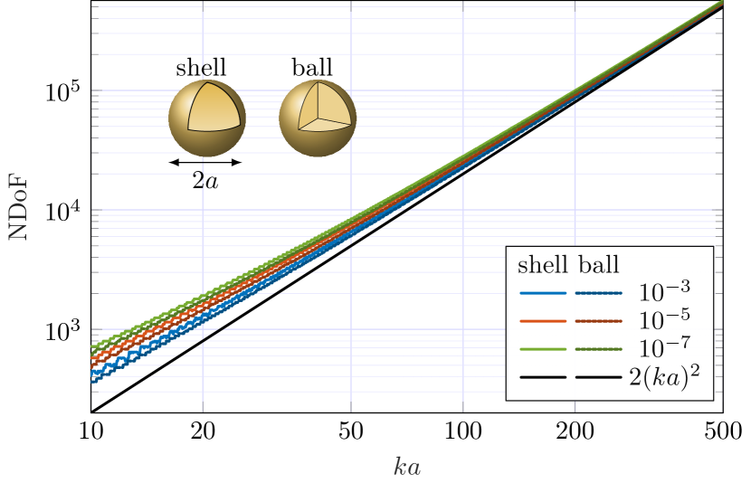
Evaluating the number of radiating spherical waves with efficiency above a given threshold, here , produces an estimate of the NDoF. Fig. 2 depicts the number of such radiating modes [8] on a spherical shell with surface resistivity and spherical ball with resistivity for . Note that copper has a surface resistivity of approximately around and a resistivity of . The results are compared with the estimate (6), and it is observed that the relative difference between the computed NDoF and decreases as . Using material losses opens a possibility to generalize the NDoF to arbitrary shaped radiators as analysed in this paper.
For arbitrary shaped regions with smooth boundary, we can interpret Weyl’s law locally, resulting in a NDoF according to (5) with surface area . However, these DoF will generally only propagate to the volume outside and not to the far field. Instead, the NDoF can be considered to propagate from the region to a slightly enlarged version of as illustrated in Fig. 3a. This short distance is considered fixed and translates to infinity many wavelength in the high-frequency limit. Also note that the NDoF is unbounded if this distance is removed.
Arbitrarily shaped closed surfaces and disjoint regions are much more complex, for which it is also apparent that there are several alternatively ways to interpret DoF, such as communication between regions [3, 21], from a region to a volume surrounding the region in Fig. 3a, and from a region to the far field in Fig. 3b. In this paper, we consider radiating NDoF interpreted as the NDoF from a region to the far field. We also interpret the NDoF from Weyl’s law (3) as the total NDoF that can propagate a short distance from the considered region, as shown in Fig. 3.
III Capacity limits and radiation modes
Treating arbitrary shaped (non-convex or non connected) regions , we can formulate a communication problem between transmitters in the region to receivers in the far field, or equivalently, on a circumscribing sphere, as shown in Fig. 3b. Current density in the transmitting region constitutes sources for the radiated field. These currents can be expanded in sufficiently large number of basis functions, with expansion coefficients collected in a column matrix [22]. Similarly, the radiated field is expanded in spherical waves [17, 18], with expansion coefficients collected in a column matrix , where denotes the projection of spherical waves onto the used basis functions [23]. The capacity (spectral efficiency) of this idealized system is determined by [8]
| (7) | ||||||
where denotes the covariance matrix of the currents, is the resistance matrix [22], and quantifies the signal-to-noise ratio (SNR) from the additive noise . In (7), the current is normalized to unit dissipated power [8]. To provide more realistic values for the capacity, physical properties can be considered. For antennas, it is common to incorporate limitations originating in the efficiency [24, 8] or bandwidth from the reactive energy around the antenna [24, 25].
The maximum capacity (7) is determined by water filling [26] for which it is convenient to rewrite (7) in a standard form by a change of variable , where is a factorization of the resistance matrix. Substituting into (7)
| (8) | ||||||
with the channel matrix . This problem is diagonalized by a singular value decomposition (SVD) of the channel matrix , i.e., (square roots of the) eigenvalues of , which can be written , where is identified as the radiation matrix [27]. Simplifying by multiplication with and setting results in an eigenvalue problem for radiation mode efficiency
| (9) |
The resistance matrix is here decomposed into the radiation matrix modelling radiated power and the material matrix modelling Ohmic or dielectric losses . Radiating modes diagonalizes (8) which solved using waterfilling over radiation mode efficiencies results in
| (10) |
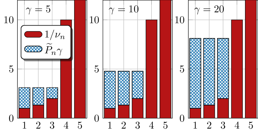
with a finite number of non-zero power levels associated with radiation modes of sufficiently high efficiency. The number of used modes depends on the signal-to-noise ratio and the distribution of the modes . Waterfilling solutions for five efficiencies and SNRs are depicted in Fig. 4. The allocation of normalized power and number of used modes depend on the SNR . For low , only the strongest modes are used, and for large , all modes are used. For modes with efficiency , the relative difference between the modes is below , and all these modes can be used for reasonable SNR . For lower efficiencies , increases rapidly, and very large SNR are needed for the water-filling solution to use these modes, as shown in Fig. 4.
The capacity (10) is solely determined by the efficiencies of the radiation modes and the signal-to-noise ratio (SNR) . Consequently, radiation modes can be regarded as fundamental physical quantities that quantify radiation properties and degrees of freedom for arbitrary-shaped objects with material losses [8].
Geometry and material properties are encapsulated within the radiation modes (9). To facilitate analysis, it is advantageous to distinguishing between the radiation contribution and the material contribution . Radiation mode eigenvalues are defined by the generalized eigenvalue problem [28]
| (11) |
with eigenvalues ordered decreasingly, i.e., , and efficiencies in (9). These modal currents are orthogonal over the material loss matrix and radiated far fields . The number of radiation modes are infinite, but they diminish rapidly as for large , similarly to the spherical waves in (6), to which they also reduce for spherical regions [27]. Radiation modes (11) are orthogonal and maximize the (Rayleigh) quotient between the radiated power and dissipated power in materials
| (12) |
which can be used to define NDoF from sufficiently efficient modes. Setting a threshold of efficiency corresponding to radiation modes , which is here used to define a NDoF for arbitrary shaped regions and material losses [8].
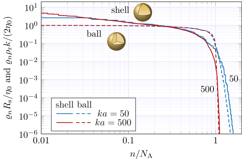
Fig. 5 depicts normalized radiation modes for spherical shells and spherical balls of the electrical sizes . The spherical shell has surface resistivity , and the spherical ball has resistivity . Both the surface and volumetric objects exhibit similar normalized radiation modes, each showing a cutoff around (6). The cutoff becomes tighter with increasing electrical size, with the case approaching a step function for the spherical ball.
Alternatively to using a threshold for the efficiency the effective NDoF [29, 30] can be used which expressed in radiation mode efficiency is
| (13) |
The effective NDoF depend on the material losses but not on a threshold level for the efficiency.
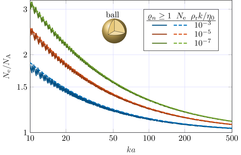
Fig. 6 shows the NDoFs in Fig. 2 normalized with estimate for the volumetric spherical region. The NDoF for electrically smaller regions are above the estimate (6) but approaches it for larger sizes. The two definitions based on and (13) agree well but the formulation oscillates due to the onset of modes at specific frequencies.
Radiation modes and hence NDoF defined by (11) or (13) can be calculated for arbitrary shapes and material parameters. Fig. 7 shows an example of NDoF for the six different shapes in Tab. I modelled by a surface resistivity . It is observed that the NDoF increase with the electrical size , with the spherical shell exhibiting the highest NDoF, followed by the solid cylinder and the corrugated cylinder, which have slightly higher NDoF than the open cylinder and connected discs. The single disc exhibits the lowest NDoF. The effective NDoF (13) produces similar results but with less oscillations. This paper demonstrates that the asymptotic number of NDoF is proportional to the electrical size of the region’s average shadow area in Tab. I, see also [10] for the corresponding number of significant characteristic modes.
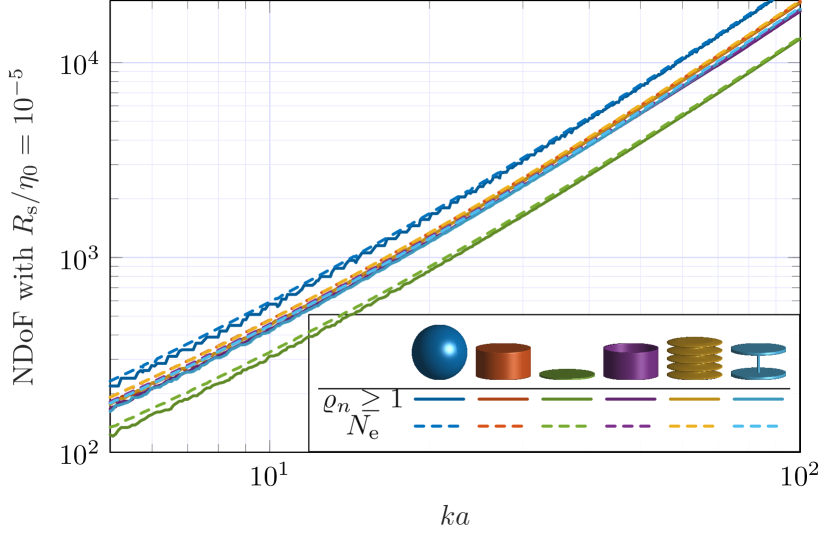
| 3.14 | 2.53 | 1.65 | 2.21 | 2.45 | 2.19 | |
| 12.6 | 10.1 | 6.59 | 10.3 | 21.9 | 11.3 | |
| 4.00 | 4.00 | 4.00 | 4.65 | 8.92 | 5.15 | |
| 2.00 | 1.00 | 0.05 | 1.00 | 1.33 | 1.00 |
IV NDoF and shadow area
Determination of NDoF from the number of radiation modes (11) greater than unity or from the effective NDoF (13) is easily achieved numerically for arbitrary shaped objects and material parameters [8], see Fig. 7. This numerical evaluation is complemented by an analytical examination, providing valuable physical insight and understanding. Specifically, it demonstrates that the radiating NDoF in the electrically large limit is proportional to the shadow area measured in squared wavelengths [10].
This proportionality can be derived using scattering or antenna theory. Here, employing antenna theory, the maximal effective area is first expressed in terms of radiation modes and subsequently related to the cross-sectional area of the object. The maximal partial effective area , and similarly the partial gain in a direction and polarization are determined from the solution of [31]
| (14) | ||||||
where is proportional to the -component of the far field in the direction , and to the corresponding partial radiation intensity [31]. The solution of (14) is
| (15) |
where the field is expand in spherical waves with expansion coefficients collected in a column matrix using [27]. Diagonalizing the optimization problem (14) using radiation modes (11) induces a change of variables with a unitary matrix having elements
| (16) |
with . Taking the average of over all directions and polarizations using the plane wave expansion [18] with spherical harmonics and results in
| (17) |
where the middle integral is, without loss of generality, evaluated for an arbitrary fixed direction as
| (18) |
and using that extends (18) to an identity dyadic. The same relation (17) holds for the orthogonal combination giving a simple identity for the average maximal effective area expressed in radiation modes
| (19) |
To estimate the number of modes, we utilize that radiation modes decay rapidly after a finite number of modes, similar to the estimate for spherical modes in (6) shown in Fig. 5. This assumption is further supported by a sum rule identity for radiation modes of homogeneous objects [27]
| (20) |
which demonstrates that radiation modes decay, as the sum of all radiation modes is fixed and proportional to the volume and inversely proportional to the resistivity.
For typical surface resistivities of metals, such as for copper around , the radiation modes approximately divide into two groups: those with and those with , see Fig. 5, resulting in efficiencies according to
| (21) |
where denotes the NDoF for the given shape and frequency. The distribution is continuous, which means that a few modes have efficiencies between 1 and 0. The transition from large to small modal efficiencies decreases with increasing electrical size, see Fig. 5.
Inserting (21) into (19) produces the estimate
| (22) |
Rewriting the affective area in the partial gain, , suggest that the NDoF can alternatively be expressed as
| (23) |
where denotes the average maximum partial gain [31]. This expression resembles the NDoF in [6] based on the maximal directivity in a fixed direction for a spherical region, but is here generalized to arbitrary shaped lossy objects.
The radiation modes are related to the geometrical structure by using that the maximal effective area in a direction approach the geometrical cross section, , in the electrically large limit [31] and similarly for the average
| (24) |
This connects the radiation modes and geometrical properties of the region with the maximal effective area (24) expressed solely in geometrical parameters producing the asymptotic NDoF
| (25) |
where denotes the total shadow area. This demonstrates that the NDoF is approximately twice to the total shadow area measured in squared wavelengths, where 2 stems from the two polarizations. Additionally, the NDoF is twice the number of significant characteristic modes [10].
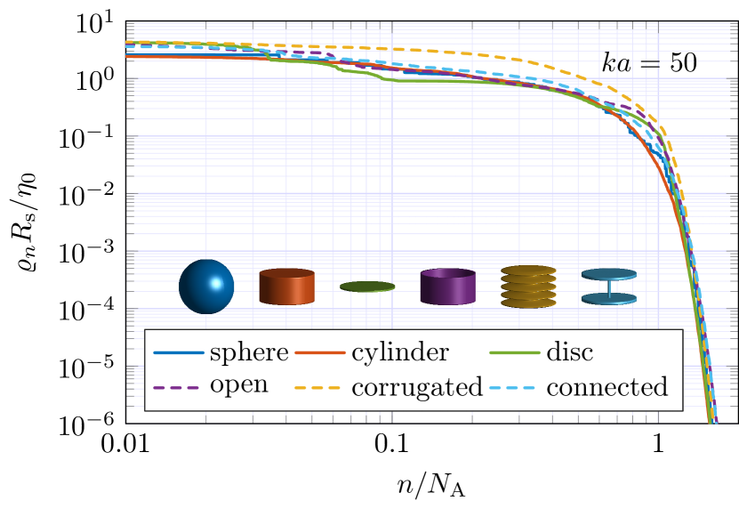
Radiation modes for six different objects are depicted in Fig. 8. The radiation mode eiganvalues are normalized with the surface resistivity , and the mode index is scaled with the NDoF, , based on the shadow area (25), as shown in Tab. I. The dominant normalized radiation modes have approximately unit magnitude, after which they rapidly decay.
The average shadow area can be determined analytically or numerically. For convex shapes it reduces to a quarter of the surface area [32]
| (26) |
This can be derived from the fact that each ray intersecting the object intersects the boundary twice [32], as shown in Fig. 9. For non-convex objects, rays might intersect the boundary more than twice. This can be interpreted as shadowing of some regions, or equivalently, that some boundary points cannot radiate undestructively over steradian to the farfield. For convex objects, the NDoF (25) simplifies as
| (27) |
This estimate agree with the cutoff for spherical regions (6) and Weyl’s law for convex shaped regions (5) but differ for non-convex shapes, see Tab. I.
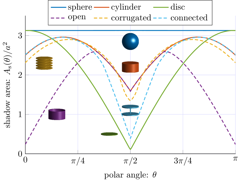
Shadow areas for the objects in Tab. I are independent of the azimuthal coordinate and plotted as function of the polar angle in Fig. 10. The sphere has for all directions. The disc is also approximately in the normal direction but much smaller seen from the side . The solid cylinder and connected discs coincide for illuminations from above, , but start to differ for illuminations from the side. The opposite holds for the cylinder compared with the open cylinder where the opening is observed from the above but not from the side. The corrugated cylinder has similar cross sectional area as the cylinder but differ for illuminations from the side where the corrugations are visible. The difference at is due to the different aspect ratio, see Tab. I. The shadow areas are bounded by which is reached for a sphere for all directions but also approximately for thin discs. The minimal values can approach zero as observed for the open cylinder at and disc at . The NDoF depends on the total shadow area (25), which is determined by integration of the curves in Fig. 10 weighted by .
The NDoF (25) depends on the material properties such as surface resistivity or bulk resistivity . Metals typically have values and below producing a distinct difference between efficient and inefficient modes as exemplified in Fig. 8 and Fig. 5. Highly resistive materials have much larger resistivity giving fewer efficient modes and hence less DoF. Materials have here for simplicity been treated as homogeneous but the formulation applies equally well for inhomogeneous regions.
The constraint based on material losses such as in (12) can alternatively be interpreted as restrictions of the amplitude of the current density. This is e.g., seen from the loss matrix of a homogeneous object, where the loss matrix separates into the resistance times the Gram matrix . Here, the least-squares norm of the current density is approximately
| (28) |
The normalized parameters and can hence be interpreted as a weight for the current norm.
V Electric and magnetic currents
The NDoFs determined in Secs. III and IV are based on the assumption of lossy non-magnetic materials or similarly, a restriction on the amplitude of the electric current . However, magnetic materials and magnetic currents are also important to consider in fully understanding the NDoF of a region. Linear magnetic materials are typically lossy and can be included in the analysis using volumetric magnetic contrast currents together with a magnetic loss matrix . Magnetic surface currents are mainly important for their use as equivalent currents used to describe the field outside a region [18].
Allowing for magnetic currents increases the NDoF compared with the solely electric case. This is particularly evident for electrical sizes where the geometrical structure is not resolved by the wavelength. NDoF of infinitely thin sheets such as planar regions do not directly follow from Weyl’s law as they do not have an inner region. Considering e.g., a planar region with only electric currents enforces a symmetry of the radiated field in the up and down directions reducing the NDoF [8]. This symmetry is broken by allowing both electric and magnetic currents on the thin sheet and hence making the structure behave as a volumetric region.
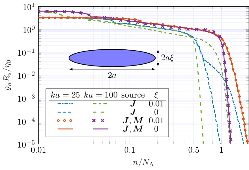
Assuming magnetic losses similar to the electric loss matrix in (10) does not affect the asymptotic NDoF (25) given by the total shadow area. Numerical evaluation of the NDoF depends however on the loss parameters and including magnetic currents increases NDoF. Fig. 11 shows the radiation modes for oblate spheroidals with aspect rations and . The magnetic surface losses are set to correspond to the electric losses.
Considering first the case with both electric, , and magnetic currents, , shown by solid curves and markers in Fig. 11. The radiation modes for oblate spheroids with and (infinitely thin disc) overlap. This is due to the negligible thickness of the oblate spheroid. The radiation modes have a cutoff around the NDoF estimate (25) based on the average shadow area with , which approaches as . The slope of for becomes steeper as increases, similar to the results for the sphere in Fig. 5. Here we also note that the disc is treated as having a top and bottom, which can equivalently be treated as half the resistivity for the disc.
The purely electric case () is more complex and shows a clear difference between the disc () and oblate spheroid (). Radiation modes for the disc show a cutoff around , indicating a halving of the NDoF. This originates from the symmetric radiation of the electric currents in the disc. The finite thickness of the oblate spheroid breaks this symmetry and increases the NDoF. The radiation modes are similar up to but differ for larger mode indices . Radiation modes for the disc decay rapidly after the cutoff around with a slope increasing with . Radiation modes for the oblate spheroid of the smaller size also have a cutoff around but then deviate from the disc modes and start to approach the traces for the and cases. The cutoff vanishes for the electrically larger case , which instead shows a cutoff as for the and cases. Note that the electric thickness of the oblate spheroid is for the cases.
Needle shaped prolate spheroidals are similarly one dimensional showing approximately a different scaling as evident from Weyl’s law (4) before their thickness is resolved.
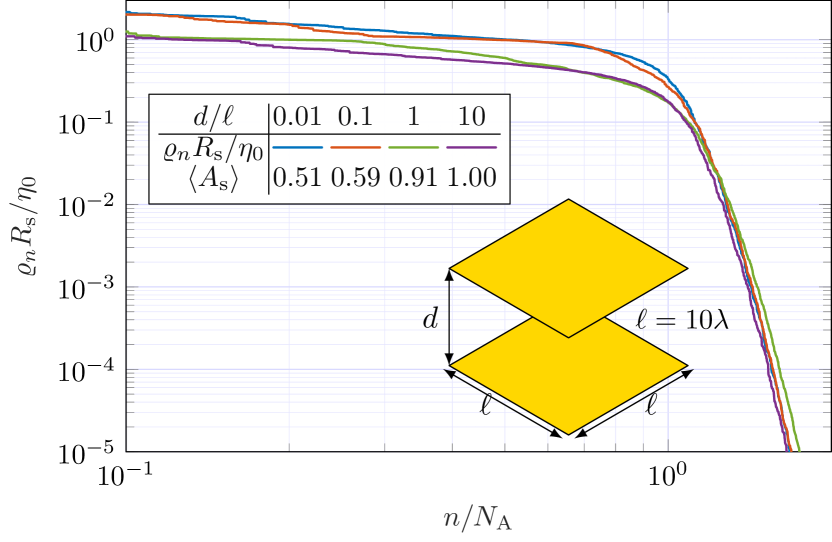
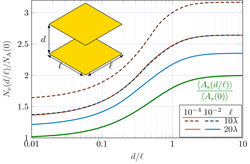
The presented derivation of the NDoFs remain valid for non-connected and multiple objects, as demonstrated by the two square plates in Figs. 12 and 13. Fig. 12 illustrates the radiation modes for two plates separated by a distance . The modal index is normalized with the asymptotic NDoF based on the average shadow area . Notably, the radiation modes exhibit a cutoff around . The shadow area can be numerically evaluated by considering the projected area of the two squares in a plane parallel to the plates. This resulting shadow area, plotted versus the distance , is illustrated in Fig. 13 by the curve , where represents the average shadow area for a single square, as shown in equation (26). As the distance increases, the average shadow area also increases and approaches as , corresponding to the NDoF of a plate with an area of .
The effective NDoFs (13) for are depicted in Fig. 13. The curves align with the trend of the asymptotic value (25) derived from the average shadow area . Moreover, they converge towards the asymptotic result as the electrical size increases, as observed for the cases.
VI Inverse source problems
The concept of NDoF for radiating systems, as analyzed in Sec. IV, also applies to inverse source problems. Consider a region composed of some linear material. By employing the equivalence principle, the radiated field can be represented by electric and magnetic surface current densities on a surface surrounding the region [33]. For simplicity, we let this surface coincide with with boundary of the region. With all sources inside , Love’s theorem or the null field condition can be used to relate the electric and magnetic currents in the inverse source problem [34, 35].
Considering for simplicity electrical currents on a PEC object. Expanding the measured field in spherical waves with expansion coefficients and adding noise to the measured field (expansion coefficients). This results in the measurement model
| (29) |
which resembles the communication model in Sec III. In inverse source problems, the source current is estimated from the observed field . The system (29) is not invertible and it is common to reformulate the system as an optimization problem or to use an SVD for a regularized solution [36].
Regularizing the inverse source problem (29) by penalizing the norm of the current density [36], e.g.,
| (30) |
where the induced metric (28) from is used for the current. Here, the regularization term has the same form as for the dissipated power in the material from the material matrix in (9), i.e., the regularization parameter mimics the normalized surface resistivity . This similarity reveals a connection between the physical bounds formulated in currents [23] and inverse source problems.
Expanding the current
| (31) |
in radiation modes (11) defined by using to diagonalize (30)
| (32) |
with the solution
| (33) |
The corresponding solution using an SVD is
| (34) |
The solutions (34) and (33) are similar for efficient radiation modes but differ for inefficient modes . Inefficient radiation modes make the noise in (29) blow up for (34) unless they are removed in the pseudo inverse related to the SVD. The (Tikhonov) regularized solution has a smoother transition where the impact of inefficient modes decreases as . The efficient modes are also the ones contributing to the NDoF.
These simple problems demonstrate the utility of NDoF derived from radiation modes and, asymptotically, from the shadow area in understanding inverse source problems. Employing the asymptotic NDoF offers a straightforward estimation of resolution in such problems. For instance, if the surface area is , then there are approximately DoFs for the current density on according to (5), while the measured data contributes approximately DoFs based on the average shadow area .
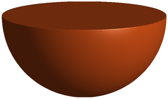
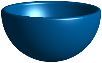
As an example, consider a hemisphere (half ball) with radius and a half spherical shell with radius and thickness , as depicted in Fig. 15. The hemisphere is convex and has a surface area and an average shadow area . The half spherical shell has an identical shadow area and an approximate surface area (assuming thin walls). This implies that the radiating NDoF asymptotically are the same for the two objects, but the non-convex bowl has a larger surface area over which the current is reconstructed. This suggests that the same NDoF are used to reconstruct the current density over different surface areas. As a consequence, this reduces the (average) resolution from approximately for the hemisphere with to approximately for the bowl.
VII Conclusions
We present a method for determining the number of degrees of freedom (NDoF) for a radiating system based on radiation modes. Asymptotically, the NDoF approaches the total shadow area measured in squared wavelengths. For convex regions, the NDoF matches the results derived from Weyl’s law. The findings extend the known expressions to arbitrary shapes, encompassing non-convex and non-connected regions. Numerical results complementing the theoretical framework and comparing them with the shadow area are provided. The derivation of the NDoF is linked to upper limits on the capacity (spectral efficiency) for a communication channel between an object and the far field, as well as to inverse source problems with measurements surrounding an object.
Appendix A Radiation modes
References
- [1] O. M. Bucci and G. Franceschetti, “On the degrees of freedom of scattered fields,” IEEE Trans. Antennas Propag., vol. 37, no. 7, pp. 918–926, 1989.
- [2] O. Bucci and T. Isernia, “Electromagnetic inverse scattering: Retrievable information and measurement strategies,” Radio science, vol. 32, no. 6, pp. 2123–2137, 1997.
- [3] R. Piestun and D. A. Miller, “Electromagnetic degrees of freedom of an optical system,” JOSA A, vol. 17, no. 5, pp. 892–902, 2000.
- [4] M. D. Migliore, “On the role of the number of degrees of freedom of the field in MIMO channels,” IEEE Trans. Antennas Propag., vol. 54, no. 2, pp. 620–628, Feb 2006.
- [5] M. Migliore, “On electromagnetics and information theory,” IEEE Trans. Antennas Propag., vol. 56, no. 10, pp. 3188–3200, Oct. 2008.
- [6] P.-S. Kildal, E. Martini, and S. Maci, “Degrees of freedom and maximum directivity of antennas: A bound on maximum directivity of nonsuperreactive antennas,” IEEE Antennas and Propagation Magazine, vol. 59, no. 4, pp. 16–25, 2017.
- [7] S. Hu, F. Rusek, and O. Edfors, “Beyond massive MIMO: The potential of data transmission with large intelligent surfaces,” IEEE Transactions on Signal Processing, vol. 66, no. 10, pp. 2746–2758, 2018.
- [8] C. Ehrenborg and M. Gustafsson, “Physical bounds and radiation modes for MIMO antennas,” IEEE Trans. Antennas Propag., vol. 68, no. 6, pp. 4302–4311, 2020.
- [9] A. Pizzo, A. de Jesus Torres, L. Sanguinetti, and T. L. Marzetta, “Nyquist sampling and degrees of freedom of electromagnetic fields,” IEEE Transactions on Signal Processing, vol. 70, pp. 3935–3947, 2022.
- [10] M. Gustafsson and J. Lundgren, “Degrees of freedom and characteristic modes,” IEEE Antennas Propag. Mag., 2024, (in press).
- [11] G. T. Di Francia, “Resolving power and information,” Josa, vol. 45, no. 7, pp. 497–501, 1955.
- [12] G. Di Francia, “Directivity, super-gain and information,” IRE Transactions on Antennas and Propagation, vol. 4, no. 3, pp. 473–478, 1956.
- [13] D. A. Hill, “Electronic mode stirring for reverberation chambers,” IEEE Trans. Electromagn. Compat., vol. 36, no. 4, pp. 294–299, 1994.
- [14] H. Weyl, “Über die asymptotische verteilung der eigenwerte,” Nachrichten von der Gesellschaft der Wissenschaften zu Göttingen, Mathematisch-Physikalische Klasse, vol. 1911, pp. 110–117, 1911.
- [15] W. Arendt, R. Nittka, W. Peter, and F. Steiner, “Weyl’s law: Spectral properties of the Laplacian in mathematics and physics,” Mathematical analysis of evolution, information, and complexity, pp. 1–71, 2009.
- [16] O. M. Bucci, C. Gennarelli, and C. Savarese, “Representation of electromagnetic fields over arbitrary surfaces by a finite and nonredundant number of samples,” IEEE Trans. Antennas Propag., vol. 46, no. 3, pp. 351–359, 1998.
- [17] R. F. Harrington, Time Harmonic Electromagnetic Fields. New York, NY: McGraw-Hill, 1961.
- [18] G. Kristensson, Scattering of Electromagnetic Waves by Obstacles. Edison, NJ: SciTech Publishing, an imprint of the IET, 2016.
- [19] J. E. Hansen, Ed., Spherical Near-Field Antenna Measurements, ser. IEE electromagnetic waves series. Stevenage, UK: Peter Peregrinus Ltd., 1988, no. 26.
- [20] J. Song and W. C. Chew, “Error analysis for the truncation of multipole expansion of vector Green’s functions,” IEEE microwave and wireless components letters, vol. 11, no. 7, pp. 311–313, 2001.
- [21] M. A. Jensen and J. W. Wallace, “Capacity of the continuous-space electromagnetic channel,” IEEE Trans. Antennas Propag., vol. 56, no. 2, pp. 524–531, 2008.
- [22] R. F. Harrington, Field Computation by Moment Methods. New York, NY: Macmillan, 1968.
- [23] M. Gustafsson and S. Nordebo, “Optimal antenna currents for Q, superdirectivity, and radiation patterns using convex optimization,” IEEE Trans. Antennas Propag., vol. 61, no. 3, pp. 1109–1118, 2013.
- [24] C. Ehrenborg and M. Gustafsson, “Fundamental bounds on MIMO antennas,” IEEE Antennas Wireless Propag. Lett., vol. 17, no. 1, pp. 21–24, January 2018.
- [25] C. Ehrenborg, M. Gustafsson, and M. Capek, “Capacity bounds and degrees of freedom for MIMO antennas constrained by Q-factor,” IEEE Trans. Antennas Propag., vol. 69, no. 9, pp. 5388–5400, 2021.
- [26] A. Paulraj, R. Nabar, and D. Gore, Introduction to Space-Time Wireless Communications. Cambridge: Cambridge University Press, 2003.
- [27] M. Gustafsson, K. Schab, L. Jelinek, and M. Capek, “Upper bounds on absorption and scattering,” New Journal of Physics, vol. 22, no. 073013, 2020.
- [28] K. R. Schab, “Modal analysis of radiation and energy storage mechanisms on conducting scatterers,” Ph.D. dissertation, University of Illinois at Urbana-Champaign, 2016.
- [29] D.-S. Shiu, G. J. Foschini, M. J. Gans, and J. M. Kahn, “Fading correlation and its effect on the capacity of multielement antenna systems,” IEEE Trans. on Communication, vol. 48, no. 3, pp. 502–513, Mar. 2000.
- [30] S. S. Yuan, Z. He, X. Chen, C. Huang, and E. Wei, “Electromagnetic effective degree of freedom of an MIMO system in free space,” IEEE Antennas and Wireless Propagation Letters, vol. 21, no. 3, pp. 446–450, 2022.
- [31] M. Gustafsson and M. Capek, “Maximum gain, effective area, and directivity,” IEEE Trans. Antennas Propag., vol. 67, no. 8, pp. 5282–5293, 2019.
- [32] V. Vouk, “Projected area of convex bodies,” Nature, vol. 162, no. 4113, pp. 330–331, 1948.
- [33] J. G. van Bladel, Electromagnetic Fields, second edition ed. Piscataway, NJ: IEEE Press, 2007.
- [34] K. Persson and M. Gustafsson, “Reconstruction of equivalent currents using a near-field data transformation – with radome applications,” Prog. Electromagn. Res., vol. 54, pp. 179–198, 2005.
- [35] J. L. A. Araque Quijano and G. Vecchi, “Field and source equivalence in source reconstruction on 3D surfaces,” Progress In Electromagnetics Research, vol. 103, pp. 67–100, 2010.
- [36] P. C. Hansen, Discrete inverse problems: insight and algorithms. Society for Industrial & Applied Mathematics, 2010, vol. 7.