PraFFL: A Preference-Aware Scheme in Fair Federated Learning
Abstract.
Fairness in federated learning has emerged as a critical concern, aiming to develop an unbiased model for any special group (e.g., male or female) of sensitive features. However, there is a trade-off between model performance and fairness, i.e., improving fairness will decrease model performance. Existing approaches have characterized such a trade-off by introducing hyperparameters to quantify client’s preferences for fairness and model performance. Nevertheless, these methods are limited to scenarios where each client has only a single pre-defined preference. In practical systems, each client may simultaneously have multiple preferences for the model performance and fairness. The key challenge is to design a method that allows the model to adapt to diverse preferences of each client in real time. To this end, we propose a Preference-aware scheme in Fair Federated Learning paradigm (called PraFFL). PraFFL can adaptively adjust the model based on each client’s preferences to meet their needs. We theoretically prove that PraFFL can provide the optimal model for client’s arbitrary preferences. Experimental results show that our proposed PraFFL outperforms five existing fair federated learning algorithms in terms of the model’s capability in adapting to clients’ different preferences.
1. Introduction
Federated learning (FL) is a distributed machine learning method that learns from multiple client data sources (mcmahan2017communication, ; tan2022towards, ), where a global model is trained cooperatively among clients without sharing data. Since the global model learns from multiple data sources, it has a stronger generalization ability across multiple clients than separately training model for each client (yuan2021we, ). However, a key concern in FL is to ensure the trained model being unbiased towards any particular groups (e.g., special races) of sensitive features (konevcny2016federated, ; hu2022fair, ; papadaki2022minimax, ). This implies that a fair model needs to treat different groups equally, such that the model’s prediction result is identical across different groups. The fairness of the model is usually measured by the differences in predictions across different groups.
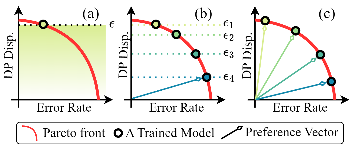
The concept of fair FL was proposed to improve the fairness of the model (zeng2021improving, ; abay2020mitigating, ; ezzeldin2023fairfed, ; pan2023fedmdfg, ). Unfortunately, many studies (gu2022privacy, ; yu2020fairness, ; du2021fairness, ) stated that fairness in FL is a trade-off issue, i.e., fairness and model performance cannot be improved simultaneously. Some existing works characterized the trade-off using hyperparameters. For example, LFT+Fedavg (abay2020mitigating, ) takes the fairness of the model as a constraint (see Figure 1(a)). FairFed (ezzeldin2023fairfed, ) introduces a hyperparameter representing a fair budget to adjust the aggregated weights when clients communicate with the server. In FAIR-FATE (salazar2023fair, ), the linear combination of model performance and fairness is taken as the optimization objective. However, these works have two main limitations. First, their determined models may not satisfy a client’s given preference over fairness and model performance. Specifically, those budget-based approaches (e.g., LFT+FedAvg and FairFed) aim to match only fairness of each client model rather than preference. For example, Figure 1(b) depicts that LFT+Fedavg has to repeatedly train the model after adjusting until the desired model is obtained. Those multi-objective-based approaches (e.g., FAIR-FATE) can obtain the desired model only when the shape of the optimal performance-fairness curve (also called Pareto front) is convex (boyd2004convex, ), while such a convexity is not necessarily satisfied in FL scenario. Second, the aforementioned approaches may not be applicable to the scenario where each client has multiple preferences. A practical example is that a social media platform (as a client in cross-silo FL) may have multiple preferences. On the one hand, some users of the social media platform hope that the recommendation system can recommend high-quality content, which means that the social media platform tends to provide a high-performance model to these users. On the other hand, other users may be more concerned about the fairness and transparency of the recommendation system, which means that the social media platform tends to provide a model with higher fairness to these users. For those aforementioned works, when each client has different requirements (i.e., fairness and preferences), their model needs to be retrained to adapt to the new requirements. Thus, their time complexity grows linearly with the number of preferences. Inspired by this, we aim to answer the following question:
How can the model (i) effectively match each client’s specific preference and (ii) be adaptively adjusted in real time based on each client’s diverse preferences?
This problem involves three technical challenges, namely establishing the connection between the two objectives (performance and fairness) and the client’s preference, alleviating the impact of data heterogeneity, and preventing the privacy leakage of client preferences. To this end, we propose a Preference-Aware scheme in Fair Federated Learning (PraFFL). Figure 1(c) shows that our method is to accurately learn a mapping from the preference vector to model performance and fairness. In this way, PraFFL enables the model to connect its fairness and performance with the corresponding preference vector. Moreover, PreFFL includes a personalized FL method to alleviate the impact of data heterogeneity. Furthermore, we introduce hypernetwork in PreFFL, which decouples each client’s preference information from other clients and the server to protect the privacy of clients. Our proposed method can provide the preference-wise model to each client within only one training. In other words, once the model is trained by PraFFL, it allows the model to adapt to each client’s preferences during the inference phase. In addition, PraFFL is theoretically proven to obtain the Pareto front within one training.
The main contributions of this paper are summarized as follows:
-
•
We present a preference learning framework, which enables the model to adapt to different preferences of each client.
-
•
We propose a PraFFL scheme to further address the three technical challenges while allowing the model to adapt to arbitrary preferences of each client.
-
•
We theoretically prove that PraFFL can provide the optimal model that meets each client’s preferences, and can learn the Pareto front in each client’s dataset.
-
•
Numerical experiments validate that our proposed method can bring 1% to 14% improvement to the best-performing baseline on four datasets in terms of the model’s capability in adapting to clients’ different preferences.
2. Related Work
There are two types of fairness in fair FL: client-based fairness (mohri2019agnostic, ; li2019fair, ; lyu2020collaborative, ; wang2021federated, ) and group-based fairness (mohri2019agnostic, ; yue2023gifair, ; deng2020distributionally, ). The purpose of client-based fairness is to equalize model performance across all clients by improving those client models with low performance. Our work mainly discusses group-based fairness, in which each client has some sensitive features. The goal of group-based fairness is to avoid discriminating against sensitive features (kamishima2012fairness, ; roh2020fairbatch, ; zhang2018mitigating, ). Many recent studies (ezzeldin2023fairfed, ; du2021fairness, ; papadaki2024federated, ) investigated how to achieve group fairness in FL. For example, an adaptive FairBatch debiasing algorithm (roh2020fairbatch, ) was proposed under the FL framework, in which the optimization problem of each client is a bi-level optimization problem. FedVal (mehrabi2022towards, ) is another simple global reweighting strategy, where the client’s aggregated weight depends on the fairness level of the model in the validation set. These approaches focus on achieving fairness among groups. However, previous studies have shown that optimizing model performance and fairness is a trade-off problem (papadaki2024federated, ; zeng2021improving, ; salazar2023fair, ; ezzeldin2023fairfed, ). To control trade-offs for model performance and fairness, the most common approach is to treat fairness as a constraint in optimizing each client’s model (galvez2021enforcing, ; zhang2020fairfl, ; du2021fairness, ). Moreover, FAIR-FATE (salazar2023fair, ) introduces a weight coefficient to linearly combine fairness and model performance as the final optimization goal. Furthermore, FairFed (ezzeldin2023fairfed, ) introduces a hyperparameter as fairness budget to adjust global reweighing. Among these reweighing algorithms, they often require clients to share the model’s fairness to calculate weights, thus leaking the clients’ privacy. Besides, some methods (hu2022federated, ; pan2023fedmdfg, ) have been proposed to find proper gradient directions between the two conflicting objectives.
Most of the above methods set hyperparameters to control the trade-off between model performance and fairness. These methods can not guarantee to meet each client’s preference. Different from previous works, our work aims to fulfill a more challenging and realistic requirement, which is to learn the model capable of adapting to each client’s arbitrary preferences.
3. Problem Formulation
3.1. Multi-Objective Learning
Let and denote the features and labels of dataset , respectively. represents the sensitive features in features . Inspired by (zeng2021improving, ), we consider a binary sensitive feature and binary classification problem, i.e., and . Now, we introduce two objectives in fair FL, i.e., model performance and fairness.
Model Performance. Let be a classifier. represents the probability that model predicts the label of feature to be one. Usually, the cross-entropy loss function is used to quantify the performance of the model in the classification problem:
| (1) |
Fairness. A classification model is fair (hardt2016equality, ) if the model prediction is independent of . That is,
| (2) |
where represents the indicator function. Eq. (2) indicates that the classifier treats two groups of the sensitive feature fairly. Based on Eq. (2), to measure the unfairness of the classifier, we define DP disparity () (zeng2021improving, ) as follows:
| (3) |
shows the difference in prediction results from the two groups. Let us deonet as the optimization goal of fairness.
Then, we convert the fair FL into a multi-objective problem to solve, which can be expressed as follows:
| (4) |
where is a two-dimensional objective vector. For presentation simplicity, in the rest of this paper, we use the terms ”solution” and ”trained model” interchangeably.
According to (papadaki2024federated, ; zeng2021improving, ), model performance and fairness are conflicting. We need to make trade-offs between these two objectives. For ease of notation, let us denote -th objective as , for all . We give the following definitions of fair FL in the context of multi-objective optimization (coello2007evolutionary, ):
Definition 3.1 (Pareto Dominance).
Let , , is said to dominate , denoted as , if and only if , for all and , for some . In addition, is said to strictly dominate , denoted as , if and only if , for all
Definition 3.2 (Pareto Optimality).
is Pareto optimal if there does not exist such that . In addition, is weakly Pareto optimal if there is no such that .
Definition 3.3 (Pareto Set/Front).
The set of all Pareto optimal solutions is called the Pareto set, and its image in the objective space is called the Pareto front.
To evaluate the quality of a solution set, a hypervolume (HV) indicator (fonseca2006improved, ) is commonly used:
Definition 3.4 (Hypervolume).
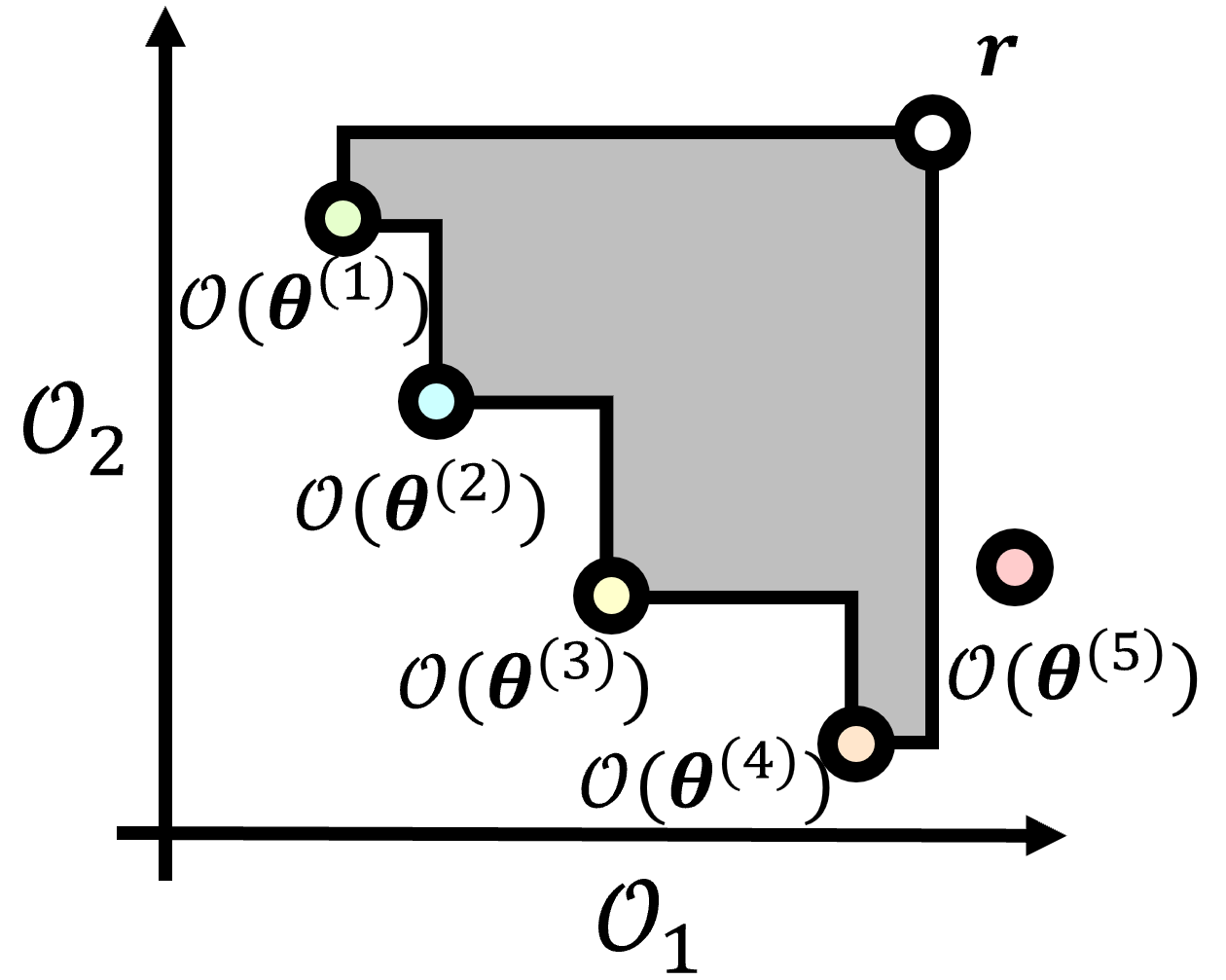
Let be a set of objective vectors given solution , []. The indicator is the two-dimensional Lebesgue measure of the region dominated by and bounded by a pre-defined reference point
Figure 2 shows the calculation of HV for a set of five solutions, where the gray area represents the HV value.
3.2. Preference Learning Framework
Optimizing multiple loss functions (Eq. (4)) simultaneously is difficult in the model. We hope that the model can adapt to given preferences. Inspired by the scalarization method in multi-objective optimization, we introduce preference vector to denote preference. We then transform the multi-objective optimization into a single-objective optimization using the preference vector. In particular, we consider a generalized setting (li2021ditto, ) where each client aims to obtain its own model . This setting is a special case that can generalize to the conventional FL case where clients aim to learn an identical global model. To enable the model to adapt to each client’s individual preferences, we concatenate () the input with the preference vector as joint features for training each client’s local model . We propose a basic preference-aware optimization objective in FL system:
| (5) |
where and is the feasible space of models. represents the dataset of client . Once the model () is optimized, the prediction results of each client’s dataset will be determined based on the client’s preferences in the inference phase. In this way, when we input different preference vectors during the inference phase, the model can automatically adjust according to each client’s given preferences.
There are three difficulties in solving Eq. (5).
-
(I)
We have no prior knowledge of the Pareto front shape. According to (boyd2004convex, ), a weight-sum optimization only works when the Pareto front is convex. Eq. (5) cannot provide all Pareto optimal solutions in the direction of preference vectors when the Pareto front is concave (illustrated in Figure 3(a)).
-
(II)
The data distribution among different clients is heterogeneous, that is, their Pareto fronts are also different (depending on each client’s data distribution).
-
(III)
Optimizing the system via Eq. (5) may leak client privacy because the preference information of each client is included in the model aggregation process of clients.
4. The Proposed Method: PraFFL
In this section, we propose a preference-aware scheme in fair FL (PraFFL). Our proposed PraFFL further addresses three difficulties in solving Eq. (5). Section 4.1 presents a preference matching approach to address difficulty (I). Furthermore, Section 4.2 introduces coupled preference to solve difficulties (II) and (III). Section 4.3 presents the details of the PraFFL scheme.
4.1. Preference Matching in PraFFL
It is difficult to provide a model whose performance and fairness fall in the direction of the client’s corresponding preference vector. To obtain a Pareto optimal solution in the direction of any given preference vector, we introduce a weighted Tchebycheff function (miettinen1999nonlinear, ) as the optimization function for each client as follows:
| (6) |
where is the ideal objective vector among two objectives, i.e., the lower bound of the two objectives. We can obtain the following promising property of problem (6):
Lemma 4.1 (Preference Consistency (miettinen1999nonlinear, )).
Given a preference vector , a solution is weakly Pareto optimal if and only if is an optimal solution of the problem (6).
Lemma 4.1 shows that given a preference vector , our method can obtain a weak Pareto optimal solution for each client if the problem (6) is minimal. Then, substituting Eq. (6) into the problem (5), the optimization problem in our system is:
| (7) |
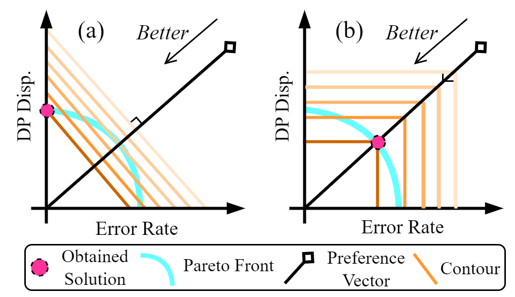
In Eq. (7), each client is optimized by the weighted Tchebycheff function, which can optimize each model towards the direction of the preference vector. Figure 3(a) shows the result obtained by linear weighting (Eq. (5)), which cannot accurately obtain the model on the preference vector. In Figure 3(b), the weight Tchebycheff optimization method we introduced can accurately obtain the model on the preference vector if Eq. (7) is minimum. In this way, we can match the preference vector for each client and learn the corresponding model. Although it can match the preference vector, it may not obtain the Pareto optimal solution because of the data heterogeneity of each client. When the server aggregates clients’ models, the aggregated model cannot simultaneously enable each client to obtain the optimal model. Therefore, we introduce personalized FL in the next section, which allows each client to obtain its own optimal model.
4.2. Preference Coupling in PraFFL
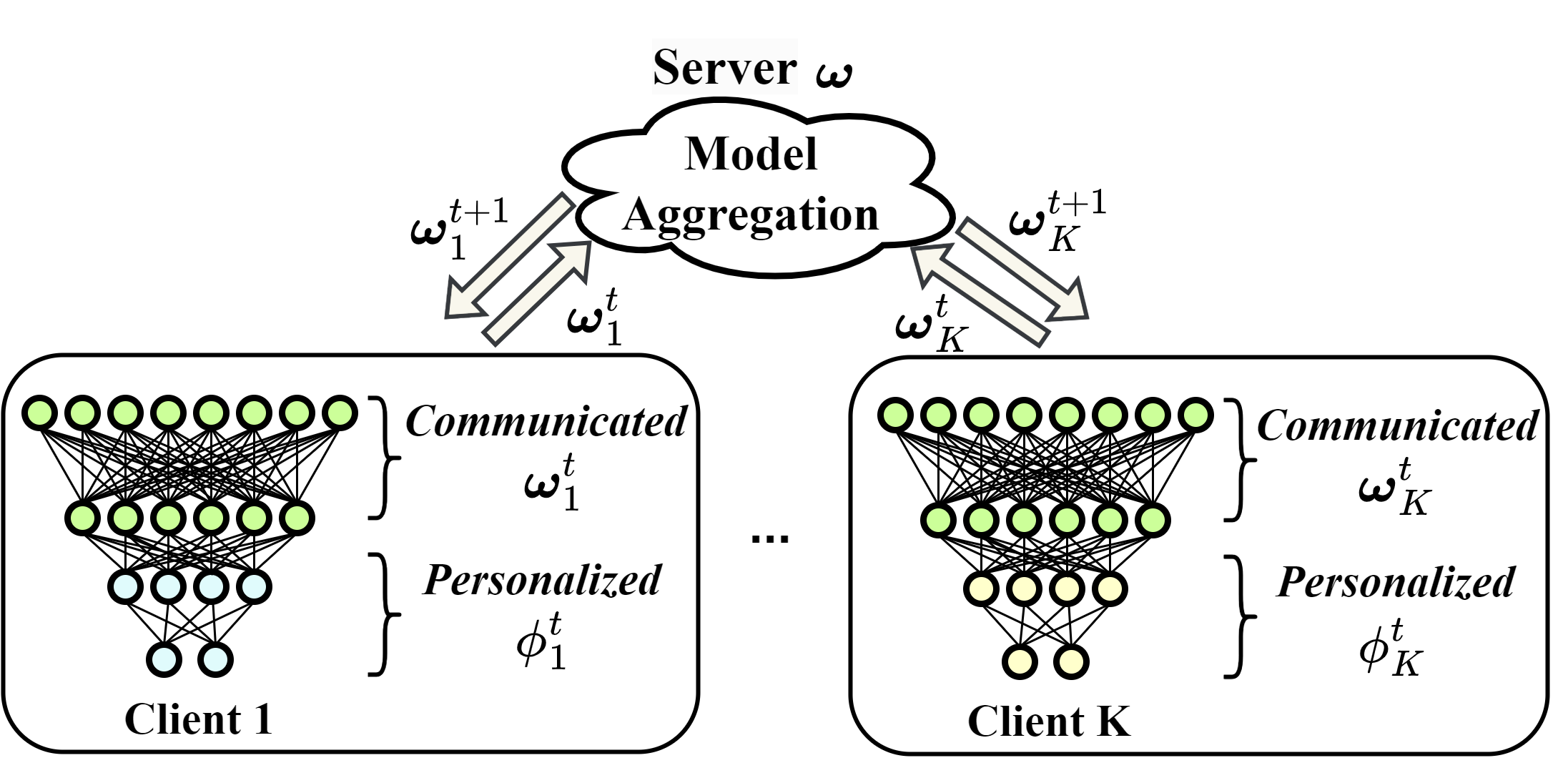
To address another two difficulties (II and III) in Section 3, we present a personalized FL framework (see Figure 4). In this framework, each client’s model is divided into two parts (communicated model and personalized model). The communicated model is the part of the model that is shared between clients. is the dimension of the data after passing through the communicated model. Each client also has a personalized model . The model of client is expressed as . The setting of the personalized model can solve difficulty (II) because each client’s personalized model is optimized according to the corresponding data distribution. The optimization goal of our personalized FL framework is as follows:
| (8a) | |||
| (8b) | |||
Our idea is to ensure the performance of the communicated model (Eq. (8b)), and then optimize the personalized model according to the given preferences (Eq. (8a)). For Eq. (8b), clients collaboratively optimize a global communicated model to minimize cross-entropy loss (performance) over their own datasets. Given in Eq. (8a), the system optimizes the personalized models of clients, considering the expected model performance and fairness over clients’ preferences.
Note that the preference information of all clients in Eq. (8) is still globally communicated (because the input of the communicated model contains the preference vectors). To further solve the difficulty (III), we introduce a hypernetwork to prevent leakage of the client’s preference information. Hypernetwork is deployed on every client. Let be a hypernetwork, which aims to learn a mapping from the preference vector to the parameters of the personalized model. Given a preference vector , the personalized model of client is as follows:
| (9) |
Based on Eq. (9), each client’s preferences are learned through hypernetowrk rather than using the concatenated operation (). Each client can directly obtain its personalized model by specifying vector (Eq. (9)). As shown in Figure 5, if the hypernetwork can be well-trained, then it can assign its output (personalized model’s parameters) that satisfy the corresponding preference to the personalized model in the inference phase. Due to the client’s preferences being learned in the hypernetwork, each client’s preference information is isolated from other clients. Therefore, hypernetwork can learn each client’s preferences while protecting the client’s preference information (addressing difficulty (III)).
To stabilize optimization of the communicated model, we need to fix the personalized model in the optimization of the communicated model. In particular, we fix the personalized model to with a fixed . Afterward, is optimized based on . The optimization problem of our system is transformed into the following:
| (10a) | |||
| (10b) | |||
Eq. (10a) aims to learn a mapping relation from preference vector distribution to a set of personalized models. So far, the three difficulties of Section 3 have been solved.
4.3. Optimization Method
We propose an optimization method to solve Eq. (10). The pseudocode of PraFFL is summarized in Algorithm 1. Specifically, there are rounds in total. In each round, a proportion of clients are selected for optimization. Then, the communicated model and the hypernetwork are optimized sequentially in each client. Each client first downloads the global communicated model as its local communicated model . To optimize the local communicated model for solving problem 10(b), client sets the personalized model to . The value of is chosen so that the personalized model is unbiased towards model performance and fairness when optimizing the local communication model. Client performs times of gradient descent algorithm for updating the communicated model at -th round (in Steps 5-6):
| (11) |
where and is the learning rate of the optimization.
After updating the communicated model, each client then optimizes the hypernetwork (in Steps 7-9). The optimization of the hypernetwork aims to enable the personalized models to adapt to different preferences. When optimizing the hypernetwork, client freezes the communicated model as in the optimization problem (10a). The optimization of the hypernetwork for client can be expressed as follows:
| (12) |
Eq. (12) is a difficult optimization problem because there are infinite possible values for . We use the Monte Carlo sampling method in stochastic optimization to optimize Eq. (12). The personalized model with steps can be further expressed as follow:
| (13) |
where , is the batch size of the sampling preference vectors and is sampled from preference vector distribution . In our work, we set to be a uniform distribution.
Once the communicated model and personalized model of participated clients in the training are updated, the participated clients send their communicated models ) to the server. Assume that the set of clients participating in the -th round is . Afterward, the server updates the communicated model with average aggregation as follows:
| (14) |
When the entire system is trained, the communicated models are the same across all clients. In contrast, the personalized model is customized based on the specific data distribution of each client. As shown in Figure 5, the client can choose arbitrary preference vectors, and the hypernetwork then provides the corresponding personalized models to the client. The client can then combine the personalized model with the communicated model, and the combined model can produce the desired results considering the client’s preference over model performance and fairness.
5. ALGORITHMIC ANALYSIS
In this section, we analyze the learning capabilities of the hypernetwork. Based on the properties of Tchebycheff function (miettinen1999nonlinear, ), we determine the following three main results:
-
•
Existence of Pareto optimality of the personalized model.
-
•
Condition of Pareto optimality of the personalized model.
-
•
The ability of the hypernetwork to find the Pareto front.
We analyze the model of an arbitrary client . Given a preference vector in problem (10a), -th objective can be expressed as over dataset . The optimization formulation is as follows:
| (15) |
At this time, a solution can be expressed as (). Since the second part is fixed, the solution is simplified by . First, we analyze the existence of the optimal personalized model. We have the following theorem:
Theorem 5.1 (Existence).
Given a preference vector , the personalized model in problem (15) has at least one Pareto optimal solution.
Proof.
Suppose that none of the optimal solution (i.e., ) in problem (15) is Pareto optimal. Let be an optimal solution to problem (15). Since we assume that it is not Pareto optimal, there must exist a personalized model which is not optimal for problem (15) but for which , and , . Therefore, we have:
| (16) |
We bring this inequality into the weighted Tchebycheff function and get the following inequality:
| (17) |
| (18) |
After we determine the existence of Pareto optimality of the personalized model, we then analyze the condition when the personalized model is Pareto optimal. We have the following theorem:
Theorem 5.2 (Pareto Optimality).
Proof.
First, we prove the first part of the theorem. Given a preference vector , let with being defined as follows:
| (19) |
We suppose that is not weakly Pareto optimal of problem (15). By the definition of Pareto optimality (Definition 2.2), there exists another personalized model such that . Therefore, we have the following inequality:
| (20) |
We bring this inequality into the weighted Tchebycheff function and get the following inequality:
| (21) |
This inequality contradicts the assumption, so is a weak Pareto optimal for problem (15).
Let’s discuss the case where the personalized model is Pareto optimal (that is, when the optimal solution of problem (15) is unique). Suppose is a unique optimal solution of problem (15), and we can get the following inequality:
| (22) |
If is not Pareto optimal, there is another solution such that . Thus, we can get the following inequality:
| (23) |
| Method | ||||||||
|---|---|---|---|---|---|---|---|---|
| PraFFL (1001 pref.) | ||||||||
| Dataset | Metrics | LFT+Ensemble | LFT+Fedavg | Agnosticfair | FedFair | FedFB | Best in ERR. | Best in DP DISP. |
| ERR. | ||||||||
| DP DISP. | ||||||||
| SYNTHETIC | HV | |||||||
| Runtime (mins.) | ||||||||
| ERR. | ||||||||
| DP DISP. | ||||||||
| COMPAS | HV | |||||||
| Runtime (mins.) | ||||||||
| ERR. | ||||||||
| DP DISP. | ||||||||
| BANK | HV | |||||||
| Runtime (mins.) | ||||||||
| ERR. | ||||||||
| DP DISP. | ||||||||
| ADULT | HV | |||||||
| Runtime (mins.) | ||||||||
Finally, we analyze the ability of the hypernetwork to find the Pareto front, and we have the following theorem:
Theorem 5.3 (Pareto Front).
Let be an optimal model for a given client’s preference. Then, there exists a preference vector such that we can obtain from problem (15).
Proof.
Let be a Pareto optimal solution. We assume that there does not exist a preference vector such that is a solution of problem (15) (i.e., is not within the domain of problem (15)). We know that , and , . We choose:
| (24) |
where is a normalizing factor. Suppose is not a solution of problem (15). In that case, there exists another solution that is a solution of problem (15), as follows:
| (25) |
This means that we have the following inequality:
| (26) |
| (27) |
Thus, dominate but we assume is a Pareto optimal solution. This contradiction completes the proof. This means that we can obtain any optimal model by optimizing hypernetowrk (). Then, the hypernetwork have the ability to find the Pareto front. ∎
6. NUMERICAL Experiments
In this section, we compare five advanced baselines (LFT+Fedavg (konecny2016federated, ), LFT+Ensemble (zeng2021improving, ), Agnosticfair (du2021fairness, ), FairFed (ezzeldin2023fairfed, ), and FedFB (zeng2021improving, )) and numerically analyze the performance of PraFFL. In particular, we analyze the performance of PraFFL on different degrees of data heterogeneity, the impact of value, and the mapping from preference vectors to the two objectives of the model. All experiments are performed with one NVIDIA GeForce RTX 2080 Ti GPU (11GB RAM). Our implementation is available at https://github.com/rG223/PraFFL.


6.1. Experimental Settings
In each experiment, we report statistical results from three runs on each dataset. We show the solutions obtained by 1001 preference vectors in the experiment (in fact, any number of solutions can be obtained through PraFFL inference as long as a corresponding number of preference vectors are given). Total communication rounds is set to 10. We include 300 epochs in one run for all fair FL algorithms. The total local epochs are set to 30 (i.e., ), and is set to 20. The batch size of data and preference vectors are set to 128 and 64, respectively. We use hypervolume (Definition 3.4) to measure the quality of the solution set obtained by each algorithm. If the suitability of the solution set to preferences is higher, the HV value is larger (the shaded area in Figure 2 is larger). Four widely used datasets are employed to conduct experiments.
-
•
SYNTHETIC (zeng2021improving, ) is an artificially generated dataset containing 3500 samples with two non-sensitive features and a binary sensitive feature.
-
•
COMPAS (barenstein2019propublica, ) has 7214 samples, 8 non-sensitive features, and 2 sensitive features (gender and race).
-
•
BANK (moro2014data, ) has 45211 samples, 13 non-sensitive features, and one sensitive feature (age).
-
•
Adult (dua2017uci, ) has 48842 samples, with 13 non-sensitive features and one sensitive feature (gender).
6.2. Main Results
Table 1 records the mean and variance of the best results within three runs. The results presented in Table 1 demonstrate that PraFFL is consistently superior to the performance of five baselines regarding HV value. Our proposed PraFFL has the best HV value in the four datasets, which are 0.971, 0.772, 1.1, and 1.01 respectively. This is because our proposed method can infer any number of personalized models, thereby obtaining more solutions with different trade-offs between model performance and fairness. Additionally, Table 1 also shows the sum of the three running times of each algorithm. Although PraFFL runs much slower than other baselines, its advantage is that once being trained, it can provide solutions for client’s arbitrary preferences in real time. Recall that other baselines require retraining the model if each client has more than one preference, and the training time increases linearly with the number of preferences. Figure 6 shows the convergence curve of each algorithm in HV value on four datasets. As the round increases, PraFFL has a significant increase in HV value, which shows that the personalized models provided by PraFFL’s hypernetwork are increasingly in line with the client’s preferences across rounds.
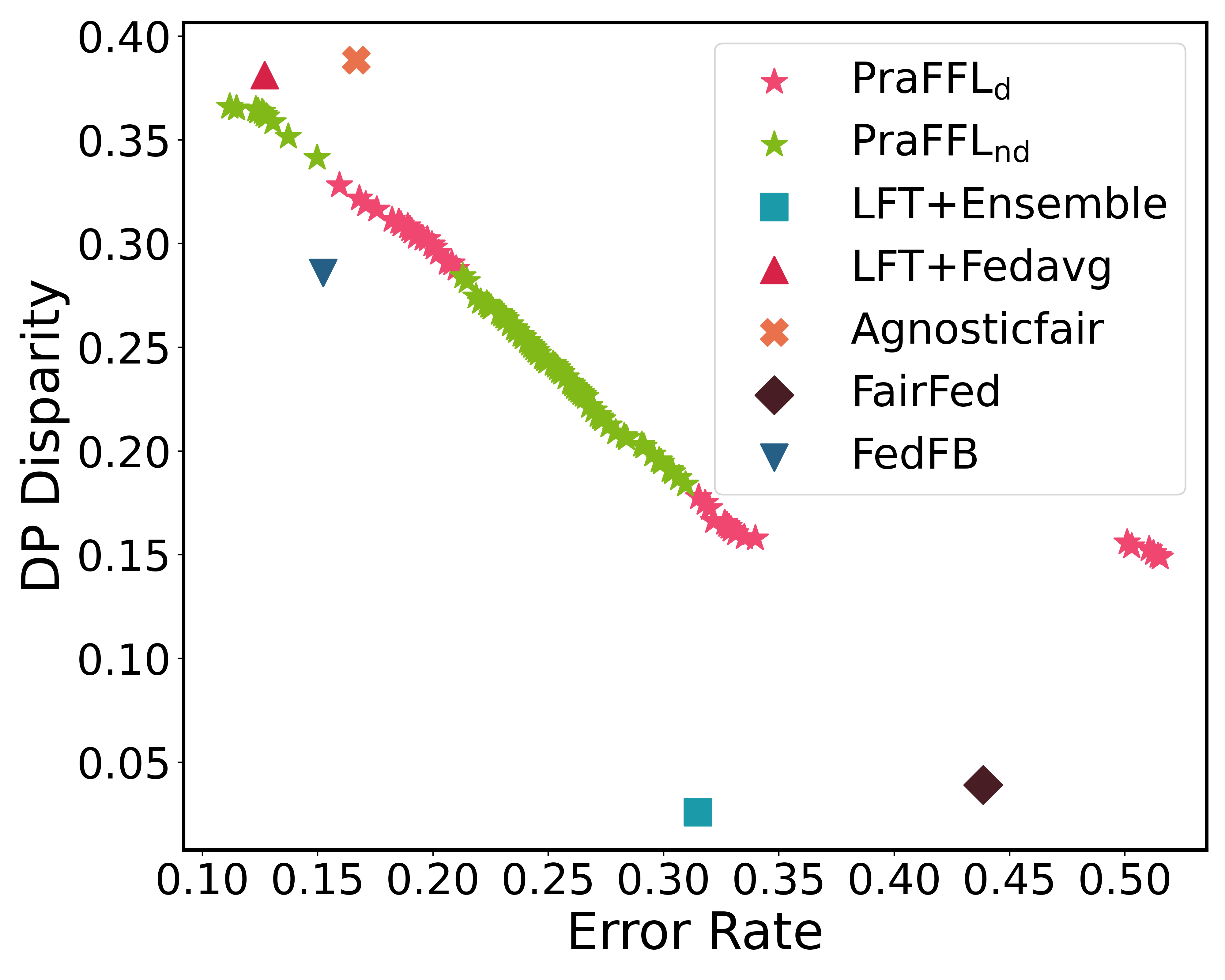
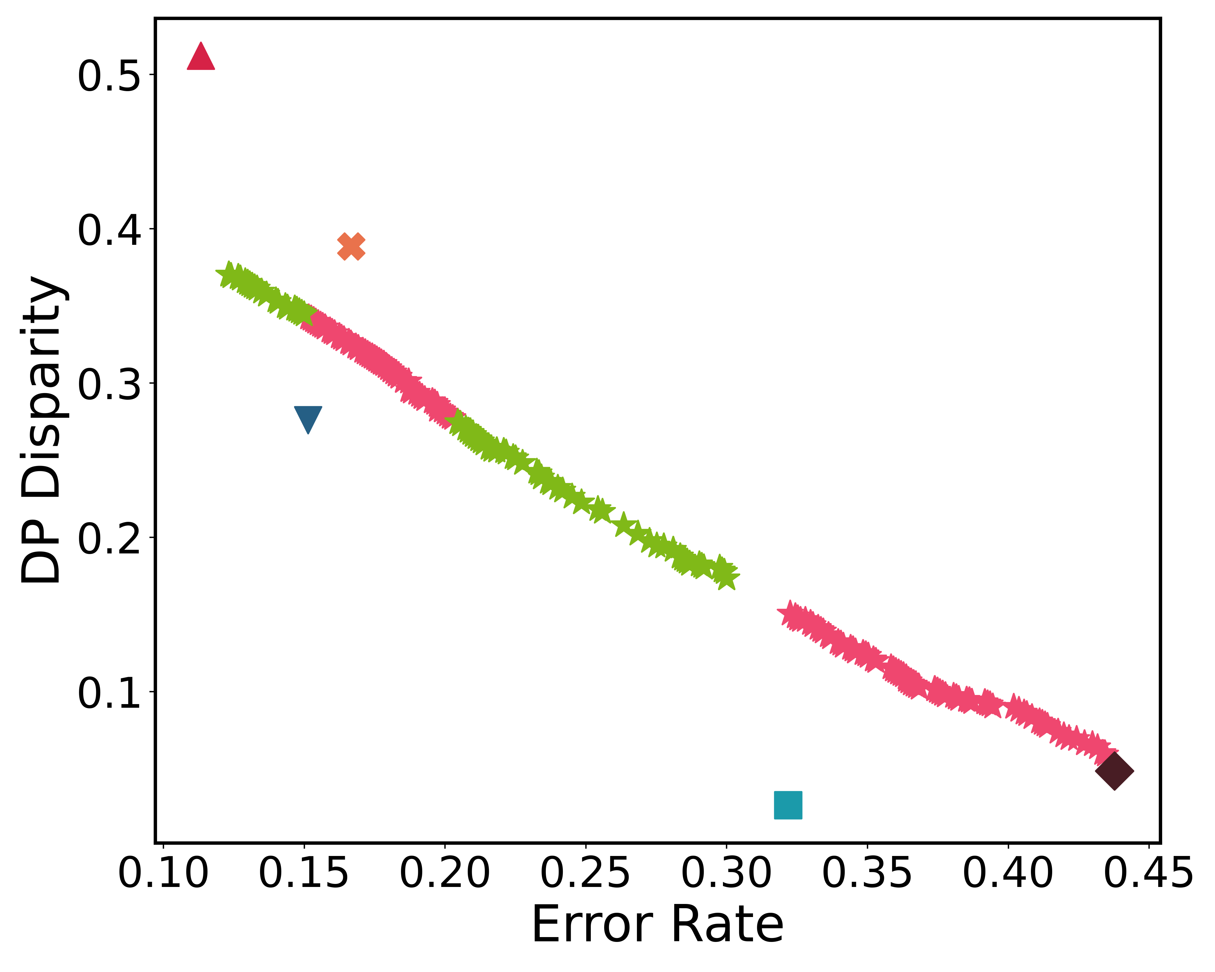
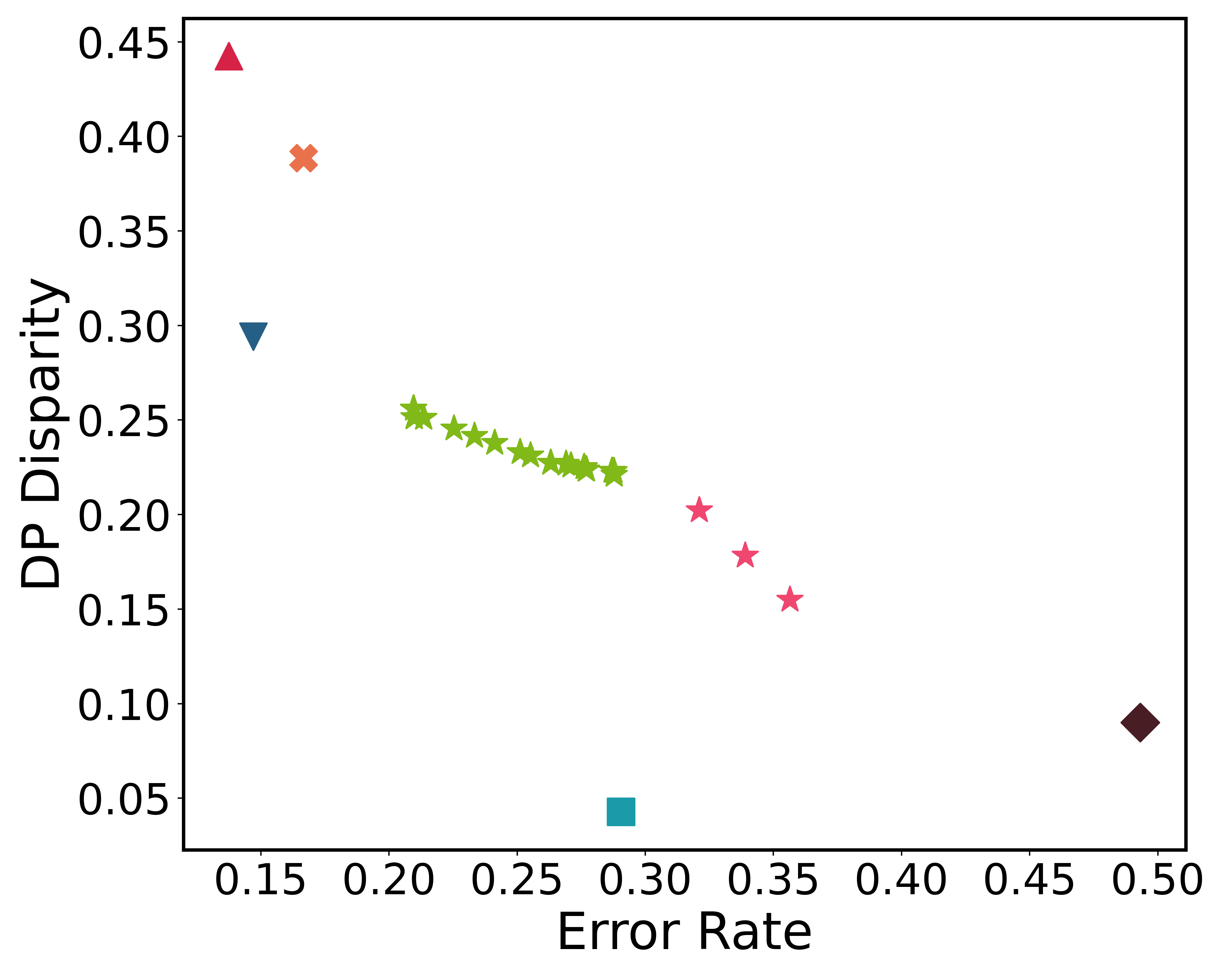
Moreover, Figure 7 shows the final solutions obtained by the baselines and the non-dominated solutions obtained by PraFFL among 1001 solutions. According to the dominance relationship in Definition 3.1, we divide the solutions obtained by PraFFL into two categories ( and ). (red stars) are inferior to some baselines in some preferences. The solution set in (green stars) is superior to other baselines (it is the best trade-off between fairness and error rate for some specific preferences). Since the solution set of PraFFL covers the optimal trade-offs for most of the client’s preferences, the solution set obtained by PraFFL is better than the solution obtained by other algorithms. The advantage of PraFFL is that it can provide arbitrary solutions for clients with only one training. In addition, we can find that PraFFL performs poorly on the COMPAS and BANK datasets, which indicates that it is difficult for PraFFL to learn all Pareto optimal solutions in some cases. There are two reasons why it is challenging to learn a superior solution set. The first is that the data distribution of the training and testing set are not exactly the same. Obtaining a superior solution set on the training set may not necessarily lead to a superior solution set on the testing set. The second reason is that our optimization goals of model performance and fairness, which are not directly equivalent to optimizing the error rate and DP Disparity. Therefore, these two reasons lead to a gap between the solution set we obtained and the optimal solution set (Pareto set), which motivates future research directions.

6.3. Sensitive Analysis
6.3.1. The effect of data heterogeneous
We examine the error rate and DP Disparity obtained by all algorithms under different heterogeneous levels on the sensitive feature. As in (zeng2021improving, ), we studied three heterogeneous scenarios. Figure 8 shows the performance of the algorithms under three different heterogeneity levels. We can observe that the solution set obtained by PraFFL at the low and medium heterogeneity is better than that at the high heterogeneity. This is because the number of solutions in is larger and more widely distributed in low and medium heterogeneity. The hypernetwork is trained by each client. If the degree of data heterogeneity increases, it will lead to another data imbalance problem, affecting the training of hypernetwork. Nonetheless, PraFFL still has some solutions in that are dominant compared to other baselines for specific preference vectors at three heterogeneity levels.
6.3.2. The effect of
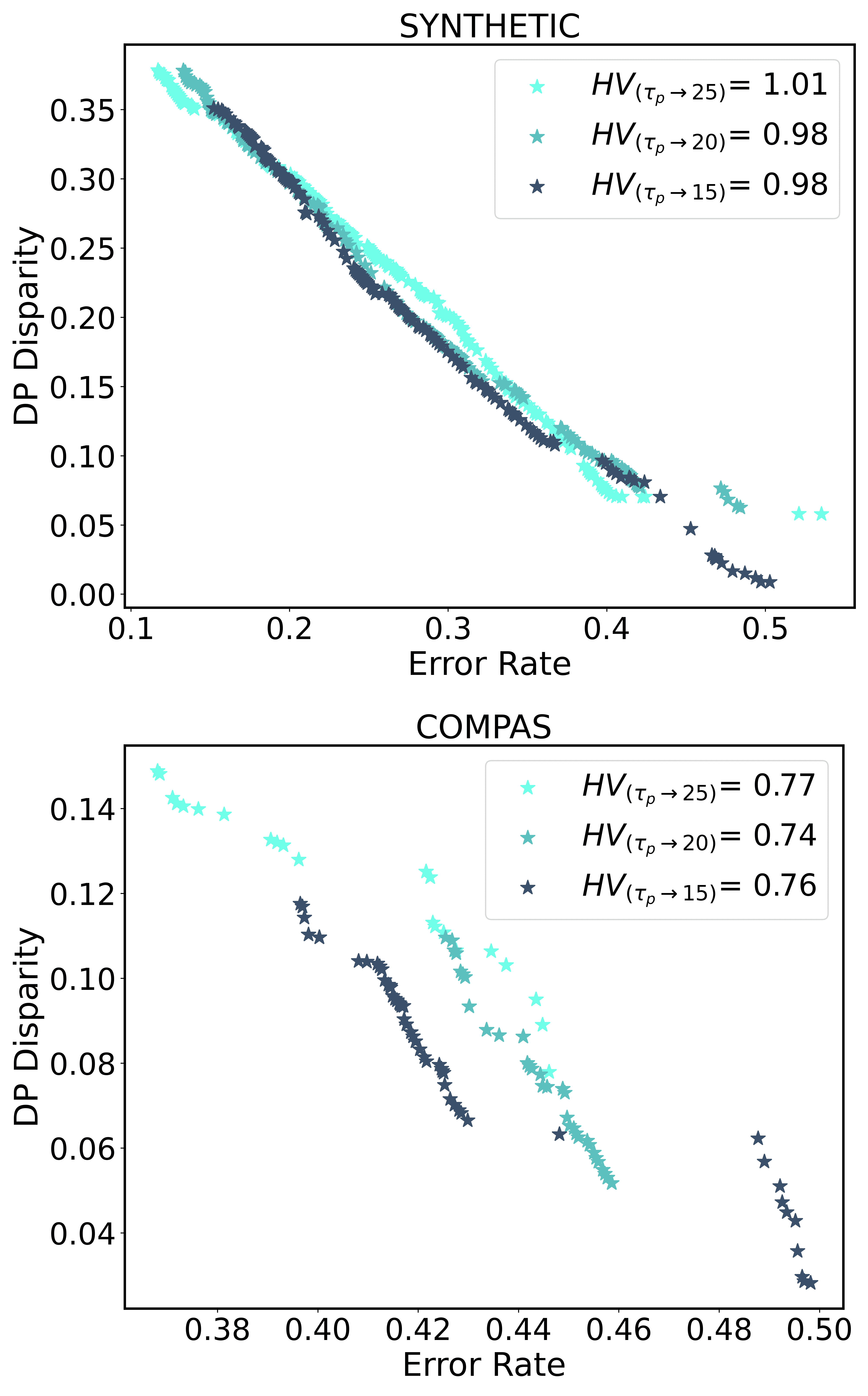
We study the impact of different values in PraFFL. The distance between the solution set and the origin is called the convergence result of the solution set, and the closer it is to the origin, the better the convergence result. As shown in Figure 9, we can find that the solution set obtained by small generally has better convergence results, but not all solutions obtained by small are better than the solution set obtained by larger . This is because a small means that the client’s communicated model is trained more times (i.e., ), which increases the overall performance of the model, but the personalized model may be underfitting for some preferences. For example, in COMPAS, the convergence result of the model is superior but the underfitting of preference vectors causes the solution set to have a large crack in the middle of the objective space (i.e., the error rate ranges from 0.43 to 0.48). Therefore, this is a trade-off problem, i.e., a large will make the overall solution set to have better fitting ability of preferences but worse convergence result, while a small will make the overall solution set converging better but worse fitting ability of preferences.
6.3.3. Different preferences of the client.
Since the solutions obtained by PraFFL on SYNTHETIC and ADULT are superior in Figure 7, we analyze the mapping relationship between the corresponding solution set of different preference vectors in these two datasets. For the simplicity of verifying the effectiveness of PraFFL, we assume that the preferences of all clients are consistent during each inference. Figure 10 shows the mapping relationship between the solution set provided by PraFFL and the client’s 1001 preferences. We can find that the solutions corresponding to different preferences are clearly distinguishable. Some of the solutions obtained by PraFFL in the ADULT dataset are dominated solutions, while the solutions in SYNTHETIC are almost all non-dominated solutions. Therefore, the solution set obtained by PraFFL on SYNTHETIC is better than the solution set obtained on ADULT. In general, PraFFL can meet most of the preference requirements of clients based on the preference vectors they provide.
7. Conclusion and Future Works
In this work, we proposed a preference-aware scheme in fair federated learning (PraFFL), which is capable of providing models with different trade-offs to every client in real time. In the training phase, our proposed PraFFL does not require the assumption that the Pareto front is convex and prevents leaking the client’s preference privacy. In the inference phase, PraFFL can infer arbitrary preferences for each client after only one training. We theoretically prove that given a client’s preference, training the hypernetwork of PraFFL can obtain the optimal personalized model and learn the entire Pareto front. Experimental results show that the solution set obtained by PraFFL on four datasets is well-performing, and the solutions obtained by PraFFL are the optimal choices for most of the client’s preferences compared to the five advanced algorithms.
Although our proposed PraFFL can achieve promising results on the four datasets, it still has room for improvement. In the first direction, the distribution of the training and testing dataset is inconsistent. A good solution set on the training dataset may not necessarily lead to a superior solution set on the testing dataset. In the second direction, the cross-entropy and fair loss function used in our work are not completely equivalent to the error rate and DP disparity, respectively. To further improve the performance of PraFFL, a possible approach in the future is to improve model generalization ability through methods such as model regularization. Another approach is to use function approximation methods to approximate the error rate and DP disparity formulation.
References
- [1] Brendan McMahan, Eider Moore, Daniel Ramage, Seth Hampson, and Blaise Aguera y Arcas. Communication-efficient learning of deep networks from decentralized data. In Artificial intelligence and statistics, pages 1273–1282. PMLR, 2017.
- [2] Alysa Ziying Tan, Han Yu, Lizhen Cui, and Qiang Yang. Towards personalized federated learning. IEEE Transactions on Neural Networks and Learning Systems, 2022.
- [3] Honglin Yuan, Warren Richard Morningstar, Lin Ning, and Karan Singhal. What do we mean by generalization in federated learning? In International Conference on Learning Representations, 2021.
- [4] Jakub Konečnỳ, H Brendan McMahan, Daniel Ramage, and Peter Richtárik. Federated optimization: Distributed machine learning for on-device intelligence. arXiv preprint arXiv:1610.02527, 2016.
- [5] Shengyuan Hu, Zhiwei Steven Wu, and Virginia Smith. Fair federated learning via bounded group loss. arXiv preprint arXiv:2203.10190, 2022.
- [6] Afroditi Papadaki, Natalia Martinez, Martin Bertran, Guillermo Sapiro, and Miguel Rodrigues. Minimax demographic group fairness in federated learning. In Proceedings of the 2022 ACM Conference on Fairness, Accountability, and Transparency, pages 142–159, 2022.
- [7] Yuchen Zeng, Hongxu Chen, and Kangwook Lee. Improving fairness via federated learning. arXiv preprint arXiv:2110.15545, 2021.
- [8] Annie Abay, Yi Zhou, Nathalie Baracaldo, Shashank Rajamoni, Ebube Chuba, and Heiko Ludwig. Mitigating bias in federated learning. arXiv preprint arXiv:2012.02447, 2020.
- [9] Yahya H Ezzeldin, Shen Yan, Chaoyang He, Emilio Ferrara, and A Salman Avestimehr. Fairfed: Enabling group fairness in federated learning. In Proceedings of the AAAI Conference on Artificial Intelligence, volume 37, pages 7494–7502, 2023.
- [10] Zibin Pan, Shuyi Wang, Chi Li, Haijin Wang, Xiaoying Tang, and Junhua Zhao. Fedmdfg: Federated learning with multi-gradient descent and fair guidance. In Proceedings of the AAAI Conference on Artificial Intelligence, volume 37, pages 9364–9371, 2023.
- [11] Xiuting Gu, Zhu Tianqing, Jie Li, Tao Zhang, Wei Ren, and Kim-Kwang Raymond Choo. Privacy, accuracy, and model fairness trade-offs in federated learning. Computers & Security, 122:102907, 2022.
- [12] Han Yu, Zelei Liu, Yang Liu, Tianjian Chen, Mingshu Cong, Xi Weng, Dusit Niyato, and Qiang Yang. A fairness-aware incentive scheme for federated learning. In Proceedings of the AAAI/ACM Conference on AI, Ethics, and Society, pages 393–399, 2020.
- [13] Wei Du, Depeng Xu, Xintao Wu, and Hanghang Tong. Fairness-aware agnostic federated learning. In Proceedings of the 2021 SIAM International Conference on Data Mining (SDM), pages 181–189. SIAM, 2021.
- [14] Teresa Salazar, Miguel Fernandes, Helder Araújo, and Pedro Henriques Abreu. Fair-fate: Fair federated learning with momentum. In International Conference on Computational Science, pages 524–538. Springer, 2023.
- [15] Stephen P Boyd and Lieven Vandenberghe. Convex optimization. Cambridge university press, 2004.
- [16] Mehryar Mohri, Gary Sivek, and Ananda Theertha Suresh. Agnostic federated learning. In International Conference on Machine Learning, pages 4615–4625. PMLR, 2019.
- [17] Tian Li, Maziar Sanjabi, Ahmad Beirami, and Virginia Smith. Fair resource allocation in federated learning. arXiv preprint arXiv:1905.10497, 2019.
- [18] Lingjuan Lyu, Xinyi Xu, Qian Wang, and Han Yu. Collaborative fairness in federated learning. Federated Learning: Privacy and Incentive, pages 189–204, 2020.
- [19] Zheng Wang, Xiaoliang Fan, Jianzhong Qi, Chenglu Wen, Cheng Wang, and Rongshan Yu. Federated learning with fair averaging. arXiv preprint arXiv:2104.14937, 2021.
- [20] Xubo Yue, Maher Nouiehed, and Raed Al Kontar. Gifair-fl: A framework for group and individual fairness in federated learning. INFORMS Journal on Data Science, 2(1):10–23, 2023.
- [21] Yuyang Deng, Mohammad Mahdi Kamani, and Mehrdad Mahdavi. Distributionally robust federated averaging. Advances in neural information processing systems, 33:15111–15122, 2020.
- [22] Toshihiro Kamishima, Shotaro Akaho, Hideki Asoh, and Jun Sakuma. Fairness-aware classifier with prejudice remover regularizer. In Machine Learning and Knowledge Discovery in Databases: European Conference, ECML PKDD 2012, Bristol, UK, September 24-28, 2012. Proceedings, Part II 23, pages 35–50. Springer, 2012.
- [23] Yuji Roh, Kangwook Lee, Steven Euijong Whang, and Changho Suh. Fairbatch: Batch selection for model fairness. arXiv preprint arXiv:2012.01696, 2020.
- [24] Brian Hu Zhang, Blake Lemoine, and Margaret Mitchell. Mitigating unwanted biases with adversarial learning. In Proceedings of the 2018 AAAI/ACM Conference on AI, Ethics, and Society, pages 335–340, 2018.
- [25] Afroditi Papadaki, Natalia Martinez, Martin Bertran, Guillermo Sapiro, and Miguel Rodrigues. Federated fairness without access to sensitive groups. arXiv preprint arXiv:2402.14929, 2024.
- [26] Ninareh Mehrabi, Cyprien de Lichy, John McKay, Cynthia He, and William Campbell. Towards multi-objective statistically fair federated learning. 2022.
- [27] Borja Rodríguez Gálvez, Filip Granqvist, Rogier van Dalen, and Matt Seigel. Enforcing fairness in private federated learning via the modified method of differential multipliers. In NeurIPS 2021 Workshop Privacy in Machine Learning, 2021.
- [28] Daniel Yue Zhang, Ziyi Kou, and Dong Wang. Fairfl: A fair federated learning approach to reducing demographic bias in privacy-sensitive classification models. In 2020 IEEE International Conference on Big Data (Big Data), pages 1051–1060. IEEE, 2020.
- [29] Zeou Hu, Kiarash Shaloudegi, Guojun Zhang, and Yaoliang Yu. Federated learning meets multi-objective optimization. IEEE Transactions on Network Science and Engineering, 9(4):2039–2051, 2022.
- [30] Moritz Hardt, Eric Price, and Nati Srebro. Equality of opportunity in supervised learning. Advances in neural information processing systems, 29, 2016.
- [31] Carlos A Coello Coello. Evolutionary algorithms for solving multi-objective problems. Springer, 2007.
- [32] Carlos M Fonseca, Luís Paquete, and Manuel López-Ibánez. An improved dimension-sweep algorithm for the hypervolume indicator. In 2006 IEEE international conference on evolutionary computation, pages 1157–1163. IEEE, 2006.
- [33] Tian Li, Shengyuan Hu, Ahmad Beirami, and Virginia Smith. Ditto: Fair and robust federated learning through personalization. In International conference on machine learning, pages 6357–6368. PMLR, 2021.
- [34] Kaisa Miettinen. Nonlinear multiobjective optimization, volume 12. Springer Science & Business Media, 1999.
- [35] Jakub Konecnỳ, H Brendan McMahan, Felix X Yu, Peter Richtárik, Ananda Theertha Suresh, and Dave Bacon. Federated learning: Strategies for improving communication efficiency. arXiv preprint arXiv:1610.05492, 8, 2016.
- [36] Matias Barenstein. Propublica’s compas data revisited. arXiv preprint arXiv:1906.04711, 2019.
- [37] Sérgio Moro, Paulo Cortez, and Paulo Rita. A data-driven approach to predict the success of bank telemarketing. Decision Support Systems, 62:22–31, 2014.
- [38] Dheeru Dua, Casey Graff, et al. Uci machine learning repository, 2017. URL http://archive. ics. uci. edu/ml, 7(1):62, 2017.