Local control on quaternionic Heisenberg group of dimension
Abstract.
We describe the quaternionic Heisenberg group in the dimension explicitly as a matrix group. We study the local control of a compatible left-invariant control system. We describe the impact of symmetries of the corresponding sub-Riemannian structure on the optimality of geodesics.
Key words and phrases:
Nilpotent algebras, Lie symmetry group, Carnot groups, sub–Riemannian geodesics1. Introduction
The three-dimensional Heisenberg group, a -step nilpotent Lie group of the filtration , is the most known and studied model in the control theory and the sub-Riemannian geometry, [1, 6]. In fact, it can be viewed as a flat, aka maximally symmetric, model in the sub-Riemannian geometry, [16]. In applications, it can be also viewed as a nilpotent approximation of the problem of the vertical rolling disk, [3, 8].
There are various generalizations to study. Clearly, it is natural to consider Heisenberg groups of higher dimensions, i.e. -step nilpotent groups of filtrations , or the products of copies of the three–dimensional Heisenberg groups, [13]. The other possibility is to focus on the free -step distributions, i.e. filtrations ; the most known and studied is the case , [15, 12, 11, 14]. We are interested in another generalization; we focus here on the Heisenberg group of the lowest possible dimension over quaternions. This leads to a specific -step nilpotent group of the filtration .
It follows from [4, 5] that quaternionic Heisenberg groups are flat models of quaternionic contact structures which are Cartan geometries modeled over . We use this fact to describe the quaternionic Heisenberg algebra of the filtration and the corresponding Carnot group via matrices from in Section 2.1. We use the Maurer-Cartan form on to define the non-holonomic distribution and the sub-Riemannian structure compatible with the group structure in Section 2.2. We study symmetries of the sub-Riemannian structure both algebraically and infinitesimally in Section 2.3.
We formulate and solve the control problem corresponding to the sub-Riemannian structure on in Section 3.1. We employ Hamiltonian viewpoint to approach the control problem and use its invariancy with respect to the group action, [1]. In particular, we describe the Hamiltonian in suitable coordinates and find corresponding control functions in Section 3.1 and we describe geodesics starting at the origin in Section 3.2.
Finally, we give our main results in Sections 4.1 and 4.2. In particular, we study the action of symmetries on geodesics and we use the action to discuss their optimality. It turns out that the behavour of geodesics is pretty analogous to classical Heisenberg, [13]. In Section 4.3 we then give some final comments and visualizations.
2. Quaternionic Heisenberg group
Let us consider the quaternion algebra and write for a quaternion . We simultaneously use the matrix representation of the quaternion as
| (1) |
2.1. Description of Lie algebra and Lie group
The quaternionic Heisenberg group is a maximally symmetric model of quaternionic structures, [5, Section 4.3.3]. These are Cartan geometries modeled on and we focus on (real) dimension , i.e. we start with . We consider the matrix representation of the Lie algebra as follows
| (2) |
for , where
denote the conjugated quaternion of and its imaginary part. Having this convention, the algebra carries a natural -grading whose components are according to the diagonal and the minus part of the grading being below the main diagonal.
We model the quaternionic Heisenberg algebra as the minus part of the grading as follows
for (real) coordinates . In particular, the Lie bracket equals to
Viewing the matrix interpretation as exponential coordinates around the origin, we can describe the corresponding group structure of the quaternionic Heisenberg group with the Lie algebra . Indeed, direct matrix computation gives
| (3) | ||||
From now on, we employ the following definition.
Definition 1.
A quaternionic Heisenberg group is a Lie group of elements of the form together with the group multiplication (3).
2.2. Maurer-Cartan form and non-holonomic distribution
Let us describe here the Maurer-Cartan form on to give a more geometric interpretation of the structure. Using the matrix description of elements of and the group operation (3), we find as
where positions are determined by the matrix representation of the quaternion (1). In particular, the corresponding coframe allows us to determine a -dimensional distribution on as follows.
Proposition 1.
The natural -dimensional left-invariant distribution on the quaternionic Heisenberg group is generated by the vector fields
where the notation stands for .
Proof.
Viewing the first columns of as a (real) coframe, one finds the vector fields as the -part of the corresponding dual frame (while the -part consists just of for ). It follows from the properties of the Maurer-Cartan form that both the frame and the coframe are left-invariant with respect to the group multiplication. ∎
The distribution is non-holonomic. Denoting
we get the following Lie algebra structure that clearly reflects the structure of and forms a -step nilpotent Lie algebra
| (4) | ||||
2.3. Sub-Riemannian structure and its symmetries
Let us consider the left-invariant sub-Riemannian metric on by declaring , , mutually orthonormal, i.e.
Altogehter, we get a left-invariant sub-Riemannian structure on the quaternionic Heisenberg group of dimension . Before we focus on the corresponding control problem, we look at symmetries of the sub-Riemannian structure.
Let us firstly employ the algebraic viewpoint. Symmetries of the quaternionic contact structure on the quaternionic Heisenberg group are (left multiplications by) elements of . On the Lie algebra level, we focus on elements of . In particular, all translations along correspond to the minus part of the grading described in (2). In addition to the translations, isotropy symmetries of the sub-Riemannian metric may appear. If so, they generally correspond to a subalgebra of , [2]. In particular, isotropy symmetries of must be contained in the zero part of the grading described in (2) and the positive part does not occur. The zero part takes form
and the real part corresponds to the grading element whose action clearly does not preserve the metric. We end up with
| (5) |
Let us remind that an infinitesimal symmetry of is a vector fields such that and for the Lie derivative . Flows of all such vector fields form a connected component of the symmetry group of . We show that the Lie algebra of infinitesimal symmetries corresponds to the algebra (5) and find explicitly the corresponding vector fields.
Proposition 2.
The Lie algebra of infinitesimal symetries of the left-invariant sub-Riemannian structure is generated by the following vector fields. Translations are generated by the vector fields
In particular, these are right-ivariant vector fields on , i.e. they commute with , . Moreover, there is an algebra of infinitesimal symmetries stabilizing the origin generated by
that forms .
Proof.
Let us roughly summarize the computation, all the details can be treated by hand or using some CAS system; we used Maple. We consider a general vector field for arbitrary functions . Computing the Lie derivative and comparing the result to zero gives a system of PDEs for unknowns ; its solution takes form
for constants , . Substituting into , computing for , contracting with defining forms and comparing with zero gives another system of PDEs. Its solution takes form
Suitable independent choices of constants , , then give all generators of the symmetry algebra.
One can check by direct computation that the first seven fields , , commute with left-invariant vector fields , , and have the same Lie bracket structure as up to the sign (compare to (4)), so they are right-invariant and generate translations. Finally, one can check that the vector fields and generate two independent Lie algebras , i.e.
so the stabilizer is isomorphic to a direct product of two Lie algebras . ∎
Our choice of generators is such that translations obviously correspond to the –block, and the translations correspond to the –block of the matrix (5). Moreover, symmetries generate corresponding to the –block, while the symmetries generate corresponding to the –block of the matrix (5). Indeed, the action of the element
for unit quaternions corresponding to results in
In the next, we denote the corresponding by the subscript or . Vector fields generating the algebra correspond to the so called left-isoclinic rotations on the distribution in the standard basis planes (there are two orthogonal planes rotating in the same orientation by the same angle considering the basis ) and identity on . Vector fields generating correspond to the so called right-isoclinic rotations on the distribution in the standard basis planes (there are two orthogonal planes rotating in the opposite orientation by the same angle considering the basis ) composed with the rotation around a standard basis vector in the double angle in -dimensional space given by .
This clearly reflects the fact that the left multiplication of a quaternion by a unit quaternion represents a left-isoclinic rotation and the right multiplication represents a right-isoclinic rotation in -dimensions, thus their compositions give arbitrary double rotations, i.e. elements of . Then the conjugation by a unit quaternion preserves a plane and gives a rotation in its orthogonal complement in the double angle. In particular, restricting to pure imaginary quaternions, it descends to a rotation in -dimensional space.
3. Local control and geodesics
3.1. Control problem and controls
Let us now discuss the control system corresponding to the sub-Riemannian structure . Considering (real) coordinates , the optimal control problem takes form
| (6) |
for and and the control with the boundary condition and for fixed points , where we minimize the energy
| (7) |
We follow here Hamiltonian concepts to approach the control system and we use its left-invariancy, [1, Sections 7 and 13]. The left-invariant vector fields , , , form a basis of and determine left-invariant coordinates on . We consider the factor here to avoid it in the subsequent equations. The corresponding left-invariant coordinates , on fibers of are given by the evaluation , and , , respectively, for arbitrary one-form on . Thus we can use , , , , as global coordinates on . In these coordinates, local minimizers, aka geodesics, are projections of the integral curves for Pontryagin’s maximum principle system corresponding to the sub-Riemannian Hamiltonian
| (8) |
to the base space .
Remark 1.
Due to the fact that we have a left-invariant Hamiltonian on a Lie group, the fiber part of the system is given by the co-adjoint action of the differential of at the origin . Viewed as a linear endomorphism in our left-invariant basis, the adjoint action takes form
| (9) |
so the co-adjoint action is given by its transpose, i.e. we mupltiply a row vector by the matrix from the right.
For we get and thus constant. For suitable constants then we denote
| (10) |
Then for we get a linear system with constant coefficients for the matrix
| (11) |
Remark 2.
The matrix reflects minus the multiplication table of the Lie algebra ; that is typical behaviour for -step filtrations, [1].
The solution of the system is given by , where is the initial value of the vector in the origin. If , then is constant. To avoid these degenerate solutions, we assume that the vector is non–zero and we denote by its length
Proposition 3.
The general solutions of the system satisfying (10) for take form
| (12) |
for orthogonal vectors
| (13) |
of the same length for
| (14) |
in the case , and for orthogonal vectors
| (15) |
of the same length for
| (16) |
in the case , where are real constants.
Proof.
The solution of the system is given by exponential of the matrix , so we need to analyze its eigenvalues and eigenvectors. It follows that there are (complex conjugated) imaginary eigenvalues both of algeraic as well as geometric multiplicity two. In the case , the corresponding eigenspace of is generated by two independent complex eigenvectors
and the eigenspace for is complex conjugate. In the case and the only non-zero contant, the corresponding eigenspace of is generated by two independent complex eigenvectors
and the eigenspace for is complex conjugate. Writting the complex solutions
respectively, utilizing the Gauss formula, decomposing both couples of these complex solutions to real and imaginary parts, considering the combinations for constants and reordering gives (12). It is a direct computation to check the orthogonality of vectors and to find their lengths. ∎
Let us discuss some properties of the solutions. In particular, the following observation holds in general. Denote the scalar product and the corresponding norm.
Proposition 4.
Let be arbitrary. Let us assume there are two vectors of the same length such that , i.e., they are othogonal. Then
for any . In particular, the curve given by the parametric formula
is a circle in the plane given by the vectors and and centered at the origin.
Proof.
Direct computation with the help of known properties of goniometric functions gives
for any and the rest follows. ∎
Corollary 1.
In the next, we assume that the vector of constants to avoud degenerate solution.
3.2. Geodesics
The base part of the system is generally given as for a geodesic , control functions and generators of the control distribution . Direct computation gives that our base system for and takes form
| (17) | ||||
where is the non-trivial submatrix of (9), i.e.
Proposition 5.
Proof.
We find the solution by a direct integration of and involving the initial condition. Then computing and subsequent direct integration gives as proposed. The description of the follows. ∎
Explicitly, denoting components of the vectors , the vector takes form
Writing explicitly using the constants and , we end up with
Let emphasize that the parametrization of geodesics is encoded in level sets of the Hamiltonian (8) of the system. In particular, the arc length parametrization corresponds to the level set , [1]. In our case, the level sets correspond to the choice that is constant (see (14) for ) and arc length parametrization corresponds to .
Finally, it turns out that for each geodesic , the component corresponds to a circle starting at the origin, while corresponds to a line. We discuss some examples in Section 4.3 in detail.
4. Symmetries and geodesics
4.1. Action symmetries on geodesics
Let us consider symmetries corresponding to the algebra that determine double rotations in the distribution around the origin in the same angle and identity on the -part. Each non-degenerate geodesic satisfies that is a linear combination of two orthogonal vectors and of the same length; thus the curve lies in the plane .
Let us remind that a Maxwell point is a point where two different geodesics meet each other with the same values of the cost functional and time (called a Maxwell time). We use the above symmetries to discuss Maxwell points of the geodesics.
Proposition 6.
For each non-degenerate geodesic starting at the origin, there is a family of geodesics of the same parametrization starting at origin all intersecting at the same Maxwell time at the Maxwell point
In particular, the geodesic is no more optimal after it reaches the time .
Remark 3.
Let us remind that the (family of) geodesics carries the arc-length parametrization for .
Proof.
The curve lies in the plane through origin . Each rotation of rotates the plane around or maps the plane to a different plane in through . In this way, we get a family of generally different geodesics through sharing the same parametrization as , and the family is the orbit of with respect to the action of , i.e.
Thus we need to focus on the coefficients in the combination. It holds for
and first such positive time appears for . Thus all geodesics from the orbit of intersect for the time .
Since the symmetries corresponding to preserve , they only impact the curve and we get identity on . So we get the proposed family of curves as the orbit of the action of the symmetries corresponding to acting on ; the rest is a direct computation. ∎
Remark 4.
Let us finally comment on symmetries corresponding to the algebra . They also determine double rotations in the distribution around the origin in the same angle. Thus if they were to induce some other restrictions on solutions, they would in particular give the same restrictions to the part of the solution. The same principle then applies to each symmetry corresponding to , thus we cannot get better estimate in this way.
4.2. Moduli space
For each geodesic and thus for the corresponding vectors , and , there is a symmetry such that
| (20) |
so we can view as a curve lying in the basis plane of the first two standard basis vectors. Thus each geodesic can be represented by the geodesic of the form
| (21) | ||||
This means that we can factorize the solution space by the action of the symmetries of to
and each geodesic (21) is the representative of a class in the quotient space.
Denote the scalar product on . The (square of the) length of the vector is an invariant of the action of . This means that together with determine (local) coordinates on . Geodesics then (locally) descend to curves of the form
| (22) | ||||
Following [12, 9], we can use these observations to discuss (locally, around the origin) critical points of the exponential map
for the Hamiltonian (8) with initial values , for , , . Moreover, the level set reflects the condition which means that the vector has the length equal to .
Due to the invariancy with respect to , we can locally factorize the exponental map to the map
| (23) | ||||
which is correctly defined if we assume that is equivalent to . Let us note that we can imagine this as working with geodesics (21) with , which manifestly leads to curves (22) for . Thus we focus on the Jacobian of the map
where we consider , and its zero points. Direct computation gives that the Jacobian equals to
| (24) | ||||
multiplied by .
Proposition 7.
The first positive zero of the function from (24) occures for .
Proof.
The function can be factorized to
and it is easy to see that the zeros of are and the zeros of
Trivially, the points where and simultaneously , i.e. the points , , are the zeros of . Observing, that is an even -function and
we see that the function has positive extremal points , each one being a zero of in the interval , . Moreover, is the point of a local minimum or maximum for odd or even, respectively. Realizing that for we can conclude that the remaining (besides those -ones) positive zeros of (and hence of ) lie strictly in the intervals , . In particular, the first (smallest) positive root of is the point . ∎
The function for has the shape as in Figure 1.
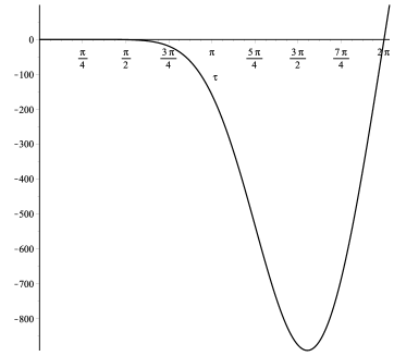
Thus for the curves (22), the time is the first conjugate time. Going to the preimage of the quotient space, the same holds for geodesics (18) of the original control problem. Then from [1, Theorem 8.72.] we get the following statement.
Corollary 2.
For geodesics (18), the time is the cut time.
4.3. Examples of orbits
Let us show here some examples of the actions on a specific geodesic. Consider the arc-length parametrized geodesic such that
Thus is the combination of and and according to (19), the vector takes form . Let us note that the geodesic corresponds to the choice of constants and remaining constants vanish.
The orbit of the geodesic by means of with respect to the action of is as follows
where we write the action of the general element (see Proposition 2 for notation) and
Remark 5.
One can see the action corresponding to as the quaternionic aka rotational grading element which reflects the behaviour on geodesics.
We see that is the first conjugate time for and we shall choose to get a family of curves intersecting at one point which is . It is the orbit for the action corresponding to which gives a family of rotations in the plane acting on . We can vizualise the circle (red) and its orbit in the plane as in Figure 2.

In particular, it manifestly reminds the geodesics on real Heisenberg group.
The action of the one-parametric family (parametrized by ) given by preserves which is the common axis of the corresponding rotations in double angle; that is why it also works for . However, the general action does not preserve the component of the solution. The orbit of for the symmetry corresponding to the choice , and parameter (from green to red) can be visualised as in Figure 3.
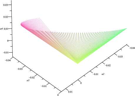
Moreover, there is a one more curve with the same property for the choice of the parameter of the form
Let us note that the action of the element (see Proposition 2 for notation), i.e. of general element of on , is as follows
and , so preserves and we get three–parametric family of curves intersecting at one point . Then it follows how it works for their composition, i.e. a general symmetry.
References
- [1] A. Agrachev, D. Barilari, U. Boscain, A comprehensive introduction to sub-Riemannian geometry. From the Hamiltonian viewpoint, Cambridge Studies in Advanced Mathematics, Vol. 181, Cambridge University Press (2020)
- [2] D. Alekseevskyi, A. Medvedev, J. Slovák, Constant curvature models in sub-Riemannian geometry. Journal of Geometry and Physics, Elsevier Science BV (2019)
- [3] A. Bellaiche, The tangent space in sub-Riemannian geometry, Sub-Riemannian Geometry (1996) 1–78
- [4] O. Biquard, Quaternionic contact structures. in Quaternionic structures in mathematics and physics (Rome, 1999) (electronic), Univ. Studi Roma ”La Sapienza”, 1999, 23–30.
- [5] A. Čap, J. Slovák, Parabolic geometries I, Background and general theory, volume 154. AMS Publishing House (2009)
- [6] E. Le Donne, Lecture notes on sub-Riemannian geometry (Carnot-Caratheodory spaces from the Lie group viewpoint), https://sites.google.com/view/enricoledonne/ Version of May 22, 2023
- [7] E. Le Donne, R. Montgomery, A. Ottazzi, P. Pansue, D. Vittone, Sard property for the endpoint map on some Carnot groups, Annales de l’Institut Henri Poincare (C) Non Linear Analysis Volume 33, Issue 6, 2016, Pages 1639-1666
- [8] J. Hrdina, A. Návrat, L. Zalabová, Symmetries in geometric control theory using Maple, Mathematics and Computers in Simulation, Volume 190, 474-493 (2021)
- [9] On symmetries of a sub-Riemannian structure with growth vector (4,7), Hrdina J., Návrat A., Zalabová L., Annali di Matematica Pura ed Applicata (2023), vol. 79, ed. 5
- [10] F. Jean, Control of Nonholonomic Systems: From Sub–Riemannian Geometry to Motion Planning. Springer (2014)
- [11] A. Montanari, G. Morbidelli, On the sub–Riemannian cut locus in a model of free two-step Carnot group. Calc. Var. 56(36) (2017)
- [12] O. Myasnichenko, Nilpotent (3, 6) sub–Riemannian problem. Journal of Dynamical and Control Systems, 8(4) (2002) 573–597
- [13] F. Monroy-Pérez, A. Anzaldo-Meneses, Optimal Control on the Heisenberg Group Journal of Dynamical and Control Systems 5(4) (1999) 473–499
- [14] F. Monroy-Pérez, A. Anzaldo-Meneses, The nilpotent sub-Riemannian problem, RR-4990, INRIA. 2003. inria-00071588
- [15] L. Rizzi, U. Serres, On the cut locus of free, step two Carnot groups, Proc. Amer. Math. Soc. 145 (2017) 5341–5357
- [16] I. Zelenko, On Tanaka’s Prolongation Procedure for Filtered Structures of Constant Type, Symmetry, Integrability and Geometry: Methods and Applications SIGMA 5(94) (2009) 1–21