Constructing and Exploring Intermediate Domains in Mixed Domain Semi-supervised Medical Image Segmentation

Supplementary Material

Dataset	Training		#Testing
	#Labeled	#Unlabeled
Fundus	20	769	271
Prostate	40	1,470	357
M&Ms	20	3,427	863

Table 1: Detailed partition information of three datasets. For each dataset, #Labeled, #Unlabeled, and #Testing indicate the number of labeled data, unlabeled data and test data, respectively.

Table 2: Comparison of different methods on Fundus dataset. + denotes we employ this method based on FixMatch. #L represents the number of labeled samples. $\uparrow$ indicates that a higher value corresponds to better performance, while $\downarrow$ suggests the opposite. The best performance is marked as bold, and the second-best is underlined.

Task		Optic Cup / Disc Segmentation
Method	#L	DC $\uparrow$				DC $\uparrow$	JC $\uparrow$	HD $\downarrow$	ASD $\downarrow$
		Domain 1	Domain 2	Domain 3	Domain 4	Avg.	Avg.	Avg.	Avg.
FixMatch	20	81.18 / 91.29	72.04 / 87.60	80.41 / 92.95	74.58 / 87.07	83.39	73.48	11.77	5.60
+FDA	20	82.59 / 92.80	74.34 / 88.63	80.08 / 92.64	77.66 / 88.99	84.72	75.33	10.38	4.82
+CutMix	20	83.62 / 92.75	71.45 / 88.69	82.09 / 92.23	80.57 / 93.30	85.59	76.32	9.61	4.71
+ClassMix	20	71.35 / 89.47	76.25 / 89.54	83.01 / 90.95	81.41 / 92.81	84.35	75.02	10.84	5.59
+CowMix	20	83.54 / 92.72	71.76 / 88.42	83.15 / 92.13	83.05 / 93.13	85.99	77.07	9.28	4.56
+FMix	20	81.88 / 92.90	72.96 / 89.10	82.41 / 92.80	82.19 / 93.33	85.95	76.80	9.26	4.52
Ours	20	83.71 / 92.96	80.47 / 89.93	84.18 / 92.97	83.71 / 93.38	87.66	79.10	8.21	3.89

Table 3: Comparison of different methods on Prostate dataset.

Task		Prostate Segmentation
Method	#L	DC $\uparrow$						DC $\uparrow$	JC $\uparrow$	HD $\downarrow$	ASD $\downarrow$
		RUNMC	BMC	HCRUDB	UCL	BIDMC	HK	Avg.	Avg.	Avg.	Avg.
FixMatch	40	83.58	69.17	73.63	79.21	56.07	84.78	74.41	65.96	24.18	14.09
+FDA	40	77.78	80.89	57.47	85.07	33.31	78.96	68.91	63.13	40.35	21.77
+CutMix	40	86.97	85.23	81.63	87.26	87.62	85.39	85.68	78.10	12.77	5.94
+ClassMix	40	85.02	69.16	69.06	85.32	43.16	76.03	71.29	60.70	57.52	28.24
+CowMix	40	86.45	85.05	83.68	87.75	88.20	84.41	85.92	78.03	12.56	5.32
+FMix	40	87.59	84.80	84.95	87.10	88.15	75.48	84.19	76.37	14.54	6.55
Ours	40	88.76	86.35	87.61	88.34	88.62	88.20	87.98	80.21	10.36	4.20

Table 4: Comparison of different methods on M&Ms dataset.

Task		LV / MYO / RV Segmentation
Method	#L	DC $\uparrow$				DC $\uparrow$	JC $\uparrow$	HD $\downarrow$	ASD $\downarrow$
		Vendor A	Vendor B	Vendor C	Vendor D	Avg.	Avg.	Avg.	Avg.
FixMatch	20	87.26 / 77.78 / 77.14	91.06 / 82.78 / 79.07	87.84 / 80.07 / 78.03	90.86 / 81.75 / 81.84	82.96	73.99	6.21	3.51
+FDA	20	85.22 / 75.40 / 76.30	89.91 / 81.59 / 78.93	85.26 / 77.32 / 74.44	89.74 / 81.60 / 80.20	81.33	72.12	7.09	4.07
+CutMix	20	86.87 / 76.90 / 80.01	91.12 / 82.04 / 79.94	87.65 / 81.31 / 80.42	90.06 / 81.73 / 81.60	83.30	74.45	5.53	2.87
+ClassMix	20	65.81 / 66.18 / 73.98	89.84 / 81.48 / 80.94	88.22 / 81.96 / 80.00	85.87 / 79.02 / 80.51	79.48	70.02	16.98	8.41
+CowMix	20	87.16 / 78.25 / 78.46	91.10 / 82.65 / 77.98	87.43 / 80.45 / 79.20	90.38 / 81.28 / 80.71	82.92	73.80	6.37	3.48
+FMix	20	86.44 / 75.16 / 79.42	91.20 / 82.84 / 79.34	87.65 / 81.05 / 80.39	90.39 / 81.72 / 81.57	83.10	73.87	5.78	2.93
Ours	20	87.77 / 76.36 / 80.65	91.48 / 83.68 / 81.46	89.25 / 82.65 / 82.27	90.91 / 82.34 / 82.86	84.31	75.18	5.15	2.42

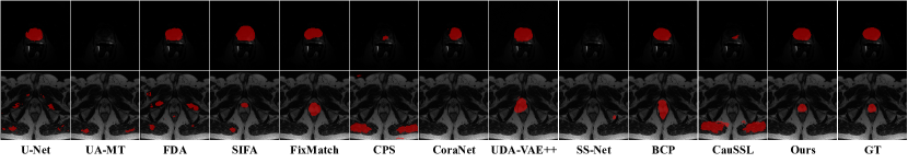
Figure 1: Visual results from Prostate dataset.

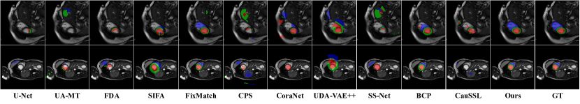
Figure 2: Visual results from M&Ms dataset. Red, green and blue represent LV, MYO and RV, respectively.

A Detailed Dataset Partition

The detailed description of the datasets is shown in Tab. 1. In our setting, labeled data share a same distribution, while unlabeled data and testing set data come from multiple domains. Fundus dataset is inherently partitioned into training and testing sets. As for Prostate and M&Ms datasets, we employed a 4:1 ratio for the division.

B Visual Results of Prostate and M&Ms

Being consistent with Fundus dataset, we present visual results under different methods for Prostate and M&Ms datasets, as illustrated in Fig. 1 and Fig. 2, respectively. Due to error accumulation caused by distribution differences, many existing state-of-the-art methods exhibit inferior segmentation capabilities on test data with the same distribution as labeled data. Their performance degrades even further when tested on data from other domains. In contrast, our method demonstrates superior segmentation performance on test data from both the same and different domains as labeled data.

C Comparison with Methods Integrating Semi-supervised Medical Image Segmentation and Domain Adaptation

Semi-supervised medical image segmentation (SSMS) methods and domain adaptation (DA) methods address distinct challenges in the Mixed Domain Semi-supervised Medical Image Segmentation scenario. For a fair comparison, we integrate various DA methods with the SSMS approach and evaluate their performance. Utilizing FixMatch [sohn2020fixmatch] as a baseline, we select FDA [yang2020fda], CutMix [yun2019cutmix], ClassMix [olsson2021classmix], CowMix [french2020milking], and FMix [harris2020fmix] to facilitate domain knowledge transfer. Specifically, FDA involves style transfer from labeled to unlabeled data, while other methods blend images using masks of different shapes. The results on three datasets are presented in Tabs. 2, 3 and 4. In experiments on the Prostate dataset, we observed a significant performance drop when combining FDA and ClassMix with FixMatch. This emphasizes the necessity of thoughtfully selecting and combining of DA strategies to address the challenges posed by domain shift in SSMS. Additionally, the combination of CutMix and FMix with FixMatch consistently achieves superior performance on all three datasets. While constructing intermediate domains through local semantic mixing helps mitigate the adverse effects of the domain gap, the intermediate domains information has not been fully utilized. Moreover, it is crucial to note that a comprehensive intermediate domains construction should not be confined solely to mixing local semantics. Taking these observations into account, our method outperforms other methods on all three datasets.