A fully implicit, asymptotic-preserving, semi-Lagrangian algorithm for the time dependent anisotropic heat transport equation

Abstract

In this paper, we extend the operator-split asymptotic-preserving, semi-Lagrangian algorithm for time dependent anisotropic heat transport equation proposed in [Chacón et al., JCP, 272, 719-746, 2014] to use a fully implicit time integration with backward differentiation formulas. The proposed implicit method can deal with arbitrary heat-transport anisotropy ratios $\chi_{\parallel}/\chi_{\perp}\ggg 1$ (with $\chi_{\parallel}$, $\chi_{\perp}$ the parallel and perpendicular heat diffusivities, respectively) in complicated magnetic field topologies in an accurate and efficient manner. The implicit algorithm is second-order accurate temporally, has favorable positivity preservation properties, and demonstrates an accurate treatment at boundary layers (e.g., island separatrices), which was not ensured by the operator-split implementation. The condition number of the resulting algebraic system is independent of the anisotropy ratio, and is inverted with preconditioned GMRES. We propose a simple preconditioner that renders the linear system compact, resulting in mesh-independent convergence rates for topologically simple magnetic fields, and convergence rates scaling as $\sim(N\Delta t)^{1/4}$ (with $N$ the total mesh size and $\Delta t$ the timestep) in topologically complex magnetic-field configurations. We demonstrate the accuracy and performance of the approach with test problems of varying complexity, including an analytically tractable boundary-layer problem in a straight magnetic field, and a topologically complex magnetic field featuring magnetic islands with extreme anisotropy ratios $(\chi_{\parallel}/\chi_{\perp}=10^{10})$.

1 Introduction

Understanding heat transport in magnetized plasmas is important for many systems of interests such as magnetic fusion, space, and astrophysical plasmas. Unfortunately, the magnetic field introduces significant heat transport anisotropy, which prevents the use of standard discretizations and solvers for parabolic/elliptic equations. In particular, heat transport is significantly faster along the field line than across it. For example, theoretical estimates, experimental measurements, and modeling suggest that the transport anisotropy in common tokamak reactors can reach extremely high values $\chi_{\parallel}/\chi_{\perp}\sim 10^{7}$ — $10^{10}$ [1, 2, 3, 4, 5, 6], where $\chi_{\parallel}$ and $\chi_{\perp}$ are thermal conductivities along and perpendicular to the magnetic field line, respectively. Such high transport anisotropy presents significant difficulties for its numerical integration. Common explicit methods would require one to resolve the fastest time scale, which is prohibitive. At the same time, implicit methods are challenged by the inversion of an almost singular operator, with condition number $\kappa$ proportional to the anisotropy ratio, $\kappa\sim\chi_{\parallel}/\chi_{\perp}$. Moreover, tiny numerical errors in the discretization of the parallel heat transport term, magnified by the anisotropy ratio, will seriously pollute subtle perpendicular dynamics of dynamical importance. High-order methods can be used to overcome error pollution [7, 8, 9, 10], but they lack monotonicity and a maximum principle [11, 12], and still lead to nearly singular parallel transport operators. It is possible to preserve monotonicity using limiters [11, 13], but at the expense of reverting to a low-order method.

Nonlocal heat closures, usually encountered in collisionless plasmas [14, 15] and stochastic magnetic fields in 3D, pose another challenge for conventional numerical methods. Almost a perfect solution for all those problems (anisotropy, nonlocal closures, and chaotic magnetic fields) in the limit $\nabla\cdot(\mathbf{B}/B)\approx 0$ was proposed for purely parallel transport [16, 17] and then extended to include perpendicular transport [18]. The key feature proposed in Refs. [16, 17, 18] is a Green’s function formulation of the heat transport equation, where parallel fast transport is resolved essentially analytically. Those methods ensure the absence of pollution due to their asymptotic preserving nature [18, 19, 20, 21] in the limit of infinite anisotropy, and grant the ability to deal with nonlocal heat closures and arbitrary magnetic field topology. Unfortunately, the algorithm proposed in Ref. [18] is based on a first-order operator splitting, and features an accuracy-based time step limitation in the presence of boundary layers in the magnetic field topology (e.g., island separatrices).

To remove this limitation, we propose in this study the extension of this algorithm to allow an implicit time integration (the possibility for such an extension was briefly formulated in [18] in an appendix) with first- and second-order backward differentiation formulas. We show by analysis that the condition number of the resulting linear matrix is independent of the anisotropy ratio $\chi_{\parallel}/\chi_{\perp}$. Preconditioned GMRES [22] is used to invert the associated algebraic system. GMRES is chosen (instead of CG) because, while formally our system (for selected sets of boundary conditions) is symmetric, we do not expect the semi-Lagrangian algorithm to remain strictly symmetric due to the interpolations performed along fields lines. Importantly, we propose a simple preconditioner that renders the linear system compact, resulting in mesh-independent convergence rates for topologically simple magnetic fields, and convergence rates scaling as $\sim(N\Delta t)^{1/4}$ (with $N$ the total mesh size and $\Delta t$ the timestep) in topologically complex magnetic-field configurations. In many applications of interest (e.g., thermonuclear magnetic fusion), the smallness of $\chi_{\perp}$ results in $\mathcal{O}(1)$ number of iterations, and therefore a practical algorithm.

Alternate AP schemes for the anisotropic transport equation have been proposed in the literature, e.g., Refs. [23, 24, 25, 26, 27]. Refs. [23, 24, 25] considered only open field lines in a time-independent context. In contrast, Ref. [27] considered only closed ones, also in a time-independent context. Ref. [26] considered the time-dependent case for open and closed magnetic fields with implicit timestepping. However, it is unclear how the approach can generalize to three dimensions (where confined stochastic field lines of infinite length may exist), and the reference employed a direct linear solver, which is known to scale very poorly with mesh refinement and with processor count in parallel environments. In contrast, our approach can be readily extended to 3D (see Refs. [16, 17] for 3D computations in the purely parallel transport case), is easily parallelizable, and scales much better with mesh refinement than either direct or unpreconditioned Krylov iterative methods.

The rest of the paper is organized as follows. In Section 2, we summarize the Lagrangian Green’s function formalism, the cornerstone of the proposed method. Next, we describe the implicit temporal discretization in Section 3. In Section 4, the spectral properties of the method are analyzed, followed by the analysis of positivity in Section 5. In Section 6, we formulate our preconditioning strategy. Numerical implementation details are provided in Section 7. Numerical tests demonstrating the merits of the new method are provided in Section 8. Finally, discussion and conclusions are provided in Sections 9 and 10, respectively.

2 The Lagrangian Green’s function formulation

For simplicity, we consider the simplest anisotropic temperature transport equation, later revising the assumptions that can be straightforwardly dropped. The anisotropic transport equation, normalized to the perpendicular transport time and length scales ($L_{\perp}$, $\tau_{\perp}=L_{\perp}^{2}/\chi_{\perp}$), reads:

$$\partial_{t}T-\frac{1}{\epsilon}\nabla_{\parallel}^{2}T=\nabla_{\perp}^{2}T+S\equiv S_{*},$$ (1)

where $T=T(t,\mathbf{x})$ is a temperature profile, $S=S(t,\mathbf{x})$ is a heat source, $S_{*}=\nabla_{\perp}^{2}T+S$ is a formal source to the purely parallel transport equation, $\epsilon=\tau_{\parallel}/\tau_{\perp}=(L_{\parallel}^{2}/\chi_{\parallel})/(L_{\perp}^{2}/\chi_{\perp})$ is the ratio between parallel and perpendicular (to the magnetic field) transport time scales, with $L,\chi$ being spatial normalization length scale and thermal conductivity, respectively. The thermal conductivity along and perpendicular to the magnetic field ($\chi_{\parallel}$ and $\chi_{\perp}$) are assumed to be constants. The generalization to non-constant conductivities is left for future work. The equation needs to be supplemented with problem-dependent boundary and initial conditions. Temperature boundary conditions at non-periodic boundaries can in principle be arbitrary. Unless otherwise stated, we consider homogeneous Dirichlet boundary conditions.

The differential operators along and perpendicular to the magnetic field $\mathbf{B}=\mathbf{b}B$ are defined as

$$\nabla_{\parallel}^{2}=\nabla\cdot(\mathbf{b}\mathbf{b}\cdot\nabla)=\left(\cancelto{\approx 0}{(\nabla\cdot\mathbf{b})}+(\mathbf{b}\cdot\nabla)\right)(\mathbf{b}\cdot\nabla)\approx(\mathbf{b}\cdot\nabla)^{2},\quad\nabla_{\perp}^{2}=\nabla^{2}-\nabla_{\parallel}^{2},$$

where $\nabla\cdot\mathbf{b}\approx 0$ is assumed. The topology of magnetic fields can otherwise be arbitrary (including stochastic magnetic fields). However, for the purpose of this paper, we will assume periodic boundary conditions or perfectly confined magnetic fields, i.e., $\mathbf{n}\cdot\mathbf{b}=0$ at boundaries, where $\mathbf{n}$ is the unit vector normal to the domain boundary.

Next, we consider the analytical solution of the anisotropic transport equation with the Green’s function formalism [18]. The formal implicit solution with initial condition $T(0,\mathbf{x})=T_{0}(\mathbf{x})=T_{0}$ is:

$$T(t,\mathbf{x})=\mathcal{G}\left(T_{0};\mathbf{x},\frac{t}{\epsilon}\right)+\int_{0}^{t}dt^{\prime}\mathcal{G}\left(S_{*};\mathbf{x},\frac{t-t^{\prime}}{\epsilon}\right),$$ (2)

where

$$\mathcal{G}\left(T_{0};\mathbf{x},t\right)=\int dsG(s,t)T_{0}\left(\mathbf{\hat{x}}(s,\mathbf{x})\right)$$ (3)

is the propagator of the homogeneous transport equation, and $G(s,t)$ is the Green’s function of the diffusion equation (see below). The integration in equation (3) is performed along the magnetic field line, which passes through $\mathbf{x}$ and is parameterized by the arc length $s$,

$$\frac{d\mathbf{\hat{x}}(s)}{ds}=\mathbf{b},\quad\mathbf{\hat{x}}(0)=\mathbf{x}.$$ (4)

In the case of perfectly confined magnetic field lines (which start and end at infinity), the Green’s function takes the form

$$G(s,t)=\frac{1}{\sqrt{4\pi t}}\exp\left(-\frac{s^{2}}{4t}\right).$$ (5)

In principle, finite magnetic-field lines and/or nonlocal heat closures can be easily incorporated by providing the appropriate Green’s function without modifying the analysis [18].

As was shown in previous studies [16, 17, 18], the Lagrangian formulation (2) features key properties, namely, that $\mathcal{G}$ is the identity on the null space of the parallel diffusion operator $\nabla_{\parallel}^{2}$ and that $\lim_{t\to\infty}\mathcal{G}$ is the projector onto that null space. These play a central role in controlling numerical pollution, and ensuring the asymptotic preserving properties of any numerical method constructed based on equation (2) when $\epsilon\rightarrow 0$. We construct an implicit time discretization of equation (2) in the next section.

3 Implicit time discretization and asymptotic-preserving property

We follow Ref. [18] and begin by constructing an implicit Euler time discretization, the first-order backward differentiation formula (BDF1). First, we rewrite equation (2) for a chosen time step with $t^{n}=n\Delta t$ and $T^{n}(\mathbf{x})=T(t^{n},\mathbf{x})$

$$T^{n+1}(\mathbf{x})=\mathcal{G}\left(T^{n};\mathbf{x},\frac{\Delta t}{\epsilon}\right)+\int_{t^{n}}^{t^{n+1}}dt^{\prime}\mathcal{G}\left(S_{*};\mathbf{x},\frac{t^{n+1}-t^{\prime}}{\epsilon}\right).$$ (6)

Next, in order to evaluate the time integral, we assume the implicit source term is constant during the time step, $S_{*}(t)\approx S_{*}(t^{n+1})\equiv S_{*}^{n+1}$, so

$$\int_{t^{n}}^{t^{n+1}}dt^{\prime}\mathcal{G}\left(S_{*};\mathbf{x},\frac{t^{n+1}-t^{\prime}}{\epsilon}\right)=\Delta t\mathcal{P}\left(S_{*}^{n+1};\mathbf{x},\frac{\Delta t}{\epsilon}\right)+\mathcal{E}_{src}^{BDF1},$$ (7)

where

$$\mathcal{P}\left(S_{*}^{n+1};\mathbf{x},\frac{\Delta t}{\epsilon}\right)=\int_{-\infty}^{+\infty}ds\mathcal{U}\left(s,\frac{\Delta t}{\epsilon}\right)S_{*}^{n+1}\left(\mathbf{\hat{x}}(s,\mathbf{x})\right),$$ (8)

and

$$\mathcal{U}\left(s,\frac{\Delta t}{\epsilon}\right)=\frac{1}{\Delta t}\int_{t^{n}}^{t^{n+1}}dt^{\prime}G\left(s,\frac{t^{n+1}-t^{\prime}}{\epsilon}\right).$$ (9)

For the Green function (5), $\mathcal{U}$ takes the form:

$$\mathcal{U}\left(s,\tau\right)=\frac{1}{\sqrt{\tau}}\left(\frac{e^{-s^{2}/4\tau}}{\sqrt{\pi}}-\frac{|s|}{2\sqrt{\tau}}\operatorname{erfc}\left(\frac{|s|}{2\sqrt{\tau}}\right)\right),$$

where $\operatorname{erfc}(x)$ is the complementary error function. The equation (7) introduces the BDF1 local discretization error, which as shown in Ref. [18] is second-order $\mathcal{E}_{src}^{BDF1}=O(\Delta t^{2})$, confirming that BDF1 is globally a first-order method. As a result, we obtain the implicit BDF1 discretization sought:

$$T(\mathbf{x})^{n+1}=\mathcal{G}\left(T^{n};\mathbf{x},\frac{\Delta t}{\epsilon}\right)+\Delta t\mathcal{P}\left(S_{*}^{n+1};\mathbf{x},\frac{\Delta t}{\epsilon}\right)+\mathcal{E}_{src}^{BDF1},$$ (10)

which can be used further to construct higher-order BDF formulas. For the purpose of this paper and to illustrate the general procedure, we derive the second-order BDF, i.e., BDF2. Rewriting equation (10) for the time step $2\Delta t$:

$$T(\mathbf{x})^{n+1}=\mathcal{G}\left(T^{n-1};\mathbf{x},\frac{2\Delta t}{\epsilon}\right)+2\Delta t\mathcal{P}\left(S_{*}^{n+1};\mathbf{x},\frac{2\Delta t}{\epsilon}\right)+4\mathcal{E}_{src}^{BDF1},$$ (11)

and subtracting equations (10), (11) such that the leading-order error terms cancel, we obtain:

$$\begin{split}T(\mathbf{x})^{n+1}&=\frac{4}{3}\mathcal{G}\left(T^{n};\mathbf{x},\frac{\Delta t}{\epsilon}\right)-\frac{1}{3}\mathcal{G}\left(T^{n-1};\mathbf{x},\frac{2\Delta t}{\epsilon}\right)\\ &+\frac{2\Delta t}{3}\left[2\mathcal{P}\left(S_{*}^{n+1};\mathbf{x},\frac{\Delta t}{\epsilon}\right)-\mathcal{P}\left(S_{*}^{n+1};\mathbf{x},\frac{2\Delta t}{\epsilon}\right)\right]+\mathcal{E}_{src}^{BDF2}.\end{split}$$ (12)

The expressions for truncation errors $\mathcal{E}_{src}^{BDF1}$ and $\mathcal{E}_{src}^{BDF2}$ were derived exactly for straight magnetic field lines in Ref. [18], and their Fourier amplitudes are:

$$\mathcal{\hat{E}}_{src}^{BDF1}(k_{\parallel},k_{\perp})=\hat{T}(k_{\parallel},k_{\perp})\min\left[\left(\frac{\Delta t}{\tau_{k}}\right)^{2},\frac{\epsilon}{k_{\parallel}^{2}\Delta t}\right],$$ (13)

$$\mathcal{\hat{E}}_{src}^{BDF2}(k_{\parallel},k_{\perp})=\hat{T}(k_{\parallel},k_{\perp})\min\left[\left(\frac{\Delta t}{\tau_{k}}\right)^{2}O(\Delta t),\frac{\epsilon}{k_{\parallel}^{2}\Delta t}\right],$$ (14)

with

$$\frac{\Delta t}{\tau_{k}}=\min\left[\Delta t\left(k_{\perp}^{2}+k_{\parallel}^{2}/\epsilon+\frac{\hat{S}(k_{\parallel},k_{\perp})}{\hat{T}(k_{\parallel},k_{\perp})}\right),1\right],$$ (15)

where $\hat{T}(k_{\parallel},k_{\perp})$ and $\hat{S}(k_{\parallel},k_{\perp})$ are Fourier components of the temperature field and the external heat source, respectively. Notice that errors in equations (13), (14) are either proportional or independent of $\epsilon$, which guarantees a bounded error for high anisotropy, $\epsilon\ll 1$, and implying that the formulation is asymptotic preserving.

4 Spectral analysis

In this section, we analyze the spectral behavior of the resulting scheme, which directly depends on the spectral properties of $\mathcal{G}$ and $\mathcal{P}$. We begin by deriving the Fourier transform of the propagation operators. Following [18], we find:

$$\int ds\mathcal{G}(f;\mathbf{x},t)e^{-ik_{\parallel}s}=\hat{f}_{k_{\parallel}}e^{-k_{\parallel}^{2}t},$$ (16)

and

$$\int ds\mathcal{P}(f;\mathbf{x},t)e^{-ik_{\parallel}s}=\hat{f}_{k_{\parallel}}\frac{1-e^{-k_{\parallel}^{2}t}}{k_{\parallel}^{2}t}.$$ (17)

4.1 Spectral properties of the linear operator $\mathcal{L}$

For the sake of brevity, we simplify notations in this section and rewrite equation (10) in the form

$$\mathcal{L}T=v,\quad\mbox{ with }\quad\mathcal{L}=\mathbb{I}+\mathcal{P}\mathbb{B},$$ (18)

where $T=T^{n+1}(\mathbf{x})$, $v$ is the right hand side that gathers contributions from terms independent of $T$ (previous time step and heat source terms), $\mathcal{P}f=\mathcal{P}(f;\mathbf{x},\Delta t/\epsilon)$, and

$$\mathbb{B}=-\Delta t\nabla_{\perp}^{2}.$$ (19)

We analyze the spectrum of the operator $\mathcal{L}$ by Fourier-analyzing (which is only rigorous in the straight magnetic field case with $\mathbf{b}$ aligned with a mesh coordinate), and using expressions (16) and (17), giving the eigenvalues:

$$\lambda=1+\frac{\beta}{\alpha}\left(1-e^{-\alpha}\right),$$

where we have introduced “conductivity scales” for parallel and perpendicular directions as:

$$\alpha=\frac{1}{\epsilon}\Delta tk_{\parallel}^{2},\quad\beta=\Delta tk_{\perp}^{2},$$ (20)

respectively. Note that $\beta$ is the eigenvalue of $\mathbb{B}$ operator, Eq. (19). It follows that, for components in the null space of the parallel transport operator ($k_{\parallel}=0$), we have:

$$\lambda_{k_{\parallel}=0}=1+\Delta tk_{\perp}^{2}.$$

Otherwise, we get:

$$\lambda_{k_{\parallel}\neq 0}=1+\mathcal{O}(\epsilon),$$

which vanishes in the limit of arbitrarily small $\epsilon$. It follows the condition number of the system matrix $\mathcal{L}$ is:

$$\kappa_{\mathcal{L}}=\frac{\lambda_{max}}{\lambda_{min}}=1+\Delta tk_{\perp}^{2}+\mathcal{O}(\epsilon),$$ (21)

which is largely independent of the small parameter $\epsilon$, and so will be the performance of the iterative method inverting it. This will be verified numerically in Sec. 8.

4.2 Linear stability

We establish next the stability of the BDF1 and BDF2 discretizations in the Von-Neumann sense. One can perform a Von Neumann temporal stability analysis, by using the usual ansatz

$$T^{n}\sim\sigma^{n}(k_{\parallel},k_{\perp})e^{i\mathbf{x}\cdot\mathbf{k}}.$$ (22)

The straightforward application of (22) to (10) and (12), using expressions (16) and (17), leads to

$$\sigma=e^{-\alpha}-\sigma\frac{\beta}{\alpha}\left(1-e^{-\alpha}\right),$$ (23)

for BDF1, and

$$\sigma=\frac{4}{3}e^{-\alpha}-\frac{1}{3\sigma}e^{-2\alpha}-\sigma\frac{\beta}{\alpha}\left(1-\frac{4}{3}e^{-\alpha}+\frac{1}{3}e^{-2\alpha}\right),$$ (24)

for BDF2. Absolute stability requires $|\sigma|<1$, which in turn demands that

$$\left|1+\frac{\beta}{\alpha}\left(1-e^{-\alpha}\right)\right|>e^{-\alpha},$$ (25)

for BDF1, and

$$\left|2\pm\sqrt{1-3\frac{\beta}{\alpha}\left(1-\frac{4}{3}e^{-\alpha}+\frac{1}{3}e^{-2\alpha}\right)}\right|>e^{-\alpha},$$ (26)

for BDF2. We can see that equations (25) and (26) are always true, as the left hand side is always greater than unity, while the right hand side is always less then unity. Hence, BDF1 and BDF2 are absolutely stable for arbitrary $\alpha$ and $\beta$ (i.e., arbitrary $\Delta t$, $k_{\parallel}$, $k_{\perp}$, and $\epsilon$).

5 Positivity

The continuum heat transport equation preserves positivity of the temperature field in the absence of sources and sinks. In this section, we show that our implicit temporal discretization applied to semi-Lagrangian formulation has robust positivity preservation properties given realistic temperature initial conditions. In order to carry out the analysis, we consider the semi-discrete context (discrete in time and continuum in space), and ignore important details of the Eulerian discretization of the isotropic Laplacian operator. In practice, positivity preservation by the semi-Lagrangian scheme will require (at the very least) having a discrete representation of the Laplacian that features a maximum principle. We assume a straight magnetic field and an infinite domain (to allow a Fourier transform). We expect that the disregarded magnetic-field curvature effects will not significantly change the positivity properties of the scheme, owing to the temperature flattening effect of fast parallel transport. Additionally, the current analysis assumes that all field lines are contained in the computational domain, thus avoiding dealing with problem-dependent boundary conditions. For the purpose of this section, we consider only the BDF1 method.

Starting with the Fourier transform of (10), we get:

$$\hat{T}^{n+1}=\frac{e^{-\alpha}}{1+\beta(\frac{1-e^{-\alpha}}{\alpha})}\hat{T}^{n},$$ (27)

where $\hat{T}$ is a Fourier transform of the temperature field. Using the convolution theorem, we can write:

$$T^{n+1}(\mathbf{x})=\int d^{3}\mathbf{x}^{\prime}\mathcal{K}(\mathbf{x}-\mathbf{x}^{\prime})T^{n}(\mathbf{x}^{\prime}),$$ (28)

where the kernel is

$$\mathcal{K}(\mathbf{x})=\frac{1}{(2\pi)^{3}}\text{Re}\left[\int d^{3}ke^{i\mathbf{k}\cdot\mathbf{x}}\frac{e^{-\alpha}}{1+\beta(\frac{1-e^{-\alpha}}{\alpha})}\right],$$ (29)

and the real part is taken for convenience (because the imaginary part is trivially zero by symmetry). After a straightforward manipulation (see C), one can simplify the integral to

$$\mathcal{K}(\mathbf{x})=\frac{1}{4\pi^{2}\Delta t}\int_{-\infty}^{\infty}dk_{\parallel}\cos(k_{\parallel}z)e^{-\alpha}\frac{\alpha}{1-e^{-\alpha}}K_{0}\left(r_{\perp}\sqrt{\frac{\alpha}{1-e^{-\alpha}}}\right),$$ (30)

where $r_{\perp}=|\mathbf{x}-\mathbf{b}\mathbf{b}\cdot\mathbf{x}|$, $z=\mathbf{b}\cdot\mathbf{x}$ is the coordinate along the magnetic field, and $K_{0}$ is the modified Bessel function of the second kind. Notice that $K_{0}(0)=\infty$, and therefore the kernel is singular when $r_{\perp}\rightarrow 0$. However, this singularity is integrable, since $K_{0}(x)\sim-\ln(x)$ for $x\sim+0$. Physically, the singularity at $r_{\perp}\rightarrow 0$ means that most of the contribution to $T^{n+1}(\mathbf{x}_{0})=T^{n+1}(x_{0},y_{0},z_{0})$ (where $x$ and $y$ are coordinates perpendicular to the magnetic field) will come from the previous time step temperature along the magnetic field line passing through $(x_{0},y_{0},z_{0})$, $T^{n}(x_{0},y_{0},z^{\prime})$. Also note that $\mathcal{K}(\mathbf{x})$ decays quickly for large $r_{\perp}$, since $K_{0}(x)\sim e^{-x}/\sqrt{x}$ for $x\rightarrow\infty$.

To study positivity, we write the kernel $\mathcal{K}$ in the form

$$\mathcal{K}(\mathbf{x})=\frac{\sqrt{\epsilon}}{2\pi^{2}(\Delta t)^{3/2}}I\left(r_{\perp},z\sqrt{\frac{\epsilon}{\Delta t}}\right),$$ (31)

with

$$I(a,b)=\int_{0}^{\infty}d\xi\cos(\xi b)e^{-\xi^{2}}\frac{\xi^{2}}{1-e^{-\xi^{2}}}K_{0}\left(a\frac{\xi}{\sqrt{1-e^{-\xi^{2}}}}\right),$$ (32)

so the positivity of $T^{n+1}$ depends only on the integral $I$, which depends on two parameters: $r_{\perp}$ and $z\sqrt{\epsilon/\Delta t}$. The numerically obtained $I$ is shown in Figure 1(a). The main feature of $I$ is an infinite logarithmic peak at $r_{\perp}=z=0$ (or $x=y=z=0$) and fast decay in all other directions. Perpendicular to the magnetic field, the kernel damps monotonically $\mathcal{K}(r_{\perp})\sim I(r_{\perp})\sim K_{0}(r_{\perp})\sim e^{-r_{\perp}}/\sqrt{r_{\perp}}$ as expected and as shown in Figure 1(b). The kernel also quickly damps in the direction along magnetic field (when $z$ increases), as shown in Figure 1(c).

If the kernel were positive everywhere, then $T^{n+1}$ would be guaranteed to be positive for any given positive $T^{n}$. However, the kernel $\mathcal{K}$ can be slightly negative in a small region around $z\sim 5\sqrt{\Delta t/\epsilon}$, as shown in Figure 1(d) (zoom of Figure 1(c)). Therefore, $T^{n+1}$ can in principle be negative for some unphysical temperature profile when, for example, temperature is zero everywhere except around $z=5\sqrt{\Delta t/\epsilon}$ (which can be a very distant region along the magnetic field line for $\epsilon\ll 1$). However, in most practical situations, the temperature field will have the form [18]:

$$T^{n}=\langle T^{n}\rangle+T_{\epsilon}^{n},$$ (33)

where $\langle T^{n}\rangle$ is a constant component along magnetic field lines (due to fast conductivity along magnetic field lines), and $T_{\epsilon}^{n}\sim\epsilon$ is a small correction. Therefore, in practice, the convolution with kernel $\mathcal{K}$ will always be positive, which ensures the positivity of the solution.

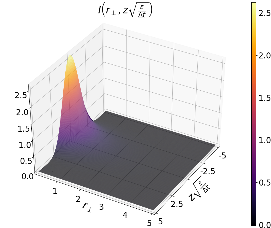
(a) $0.1<r_{\perp}<5$, $-5<z\sqrt{\epsilon/\Delta t}<5$.

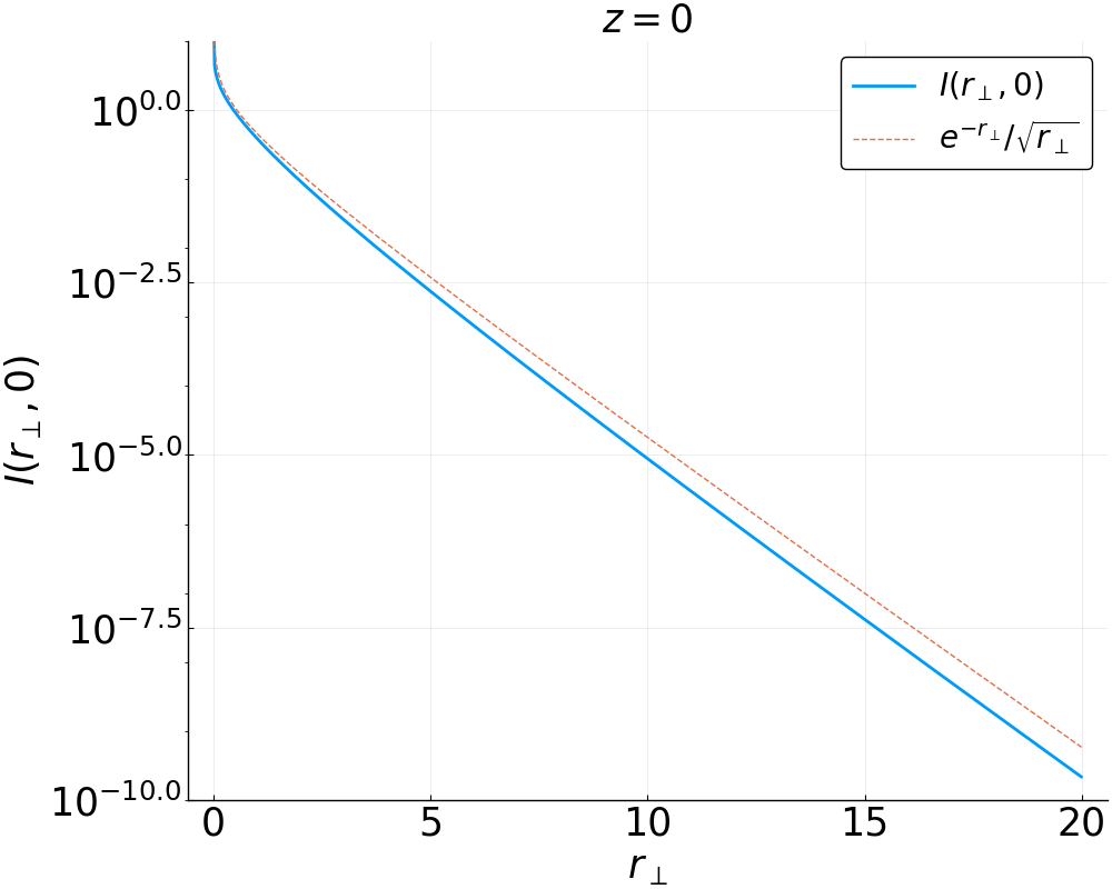
(b) $10^{-4}<r_{\perp}<20$, $z=0$.

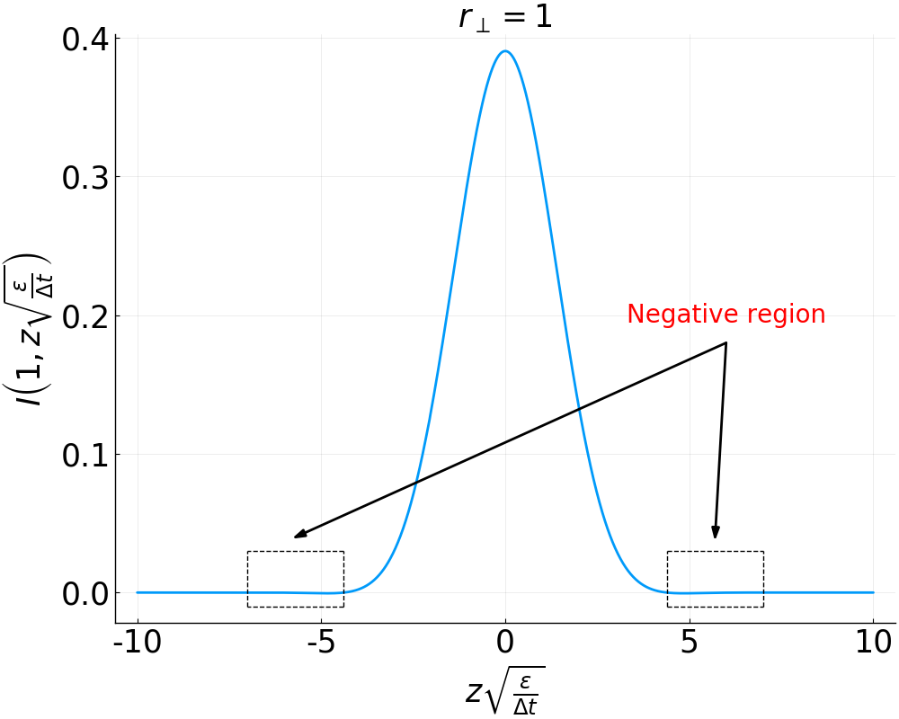
(c) $r_{\perp}=1$, $-10<z\sqrt{\epsilon/\Delta t}<10$.

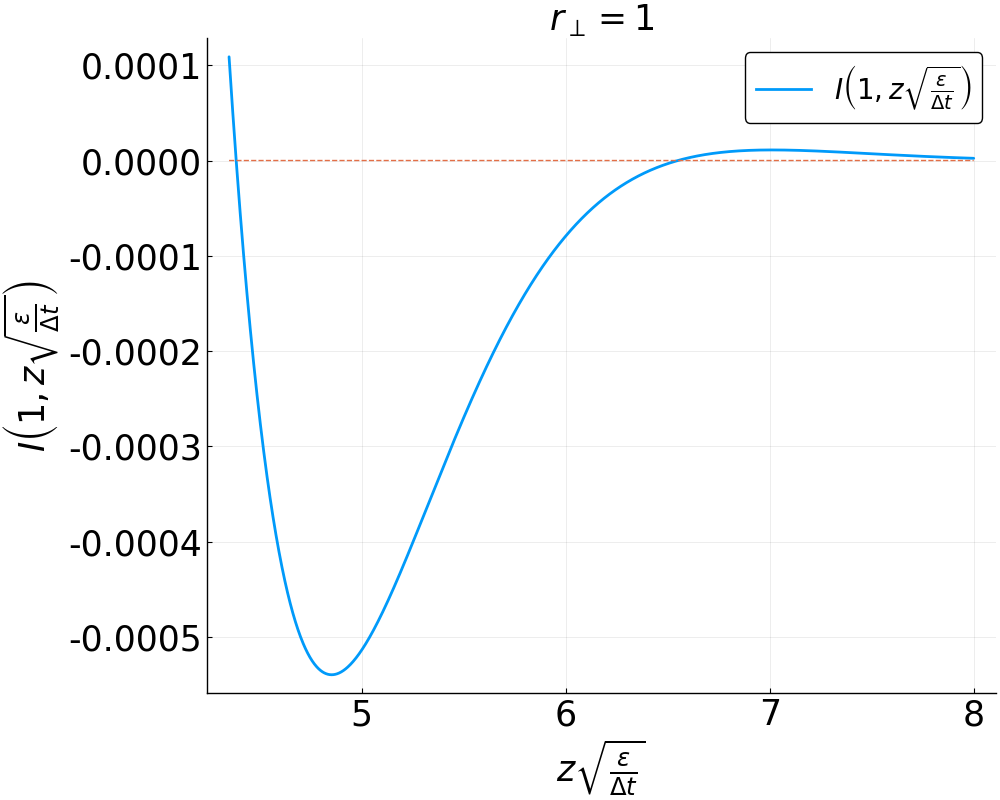
(d) $r_{\perp}=1$, $4.35<z\sqrt{\epsilon/\Delta t}<8$.

Figure 1: Numerically evaluated integral kernel (32)

6 Preconditioning strategy

Equations (10) and (12) are implicit. Thus, one needs to invert them at every time step. However, a matrix representation for any given discretization of the operators $\mathcal{G}$ and $\mathcal{P}$ for arbitrary $\mathbf{B}$ is not known beforehand, and would be extremely difficult to construct. Therefore, it is advantageous to use robust matrix-free Krylov methods such as GMRES (generalized minimal residuals) [22].

In general, the convergence of Krylov methods is sensitive to the condition number of the linear operator. Indeed, the number of GMRES (or CG for SPD systems) iterations scales as $N_{i}\sim\sqrt{\kappa}$ [28]. However, for compact operators stemming from integral equations, this performance estimate can be quite pessimistic, and in practice performance of GMRES in particular can be found to be mesh independent [29]. Our preconditioning strategy is to render the right-preconditioned linear operator $\mathcal{L}\mathcal{M}^{-1}=(\mathbb{I}+\mathcal{P}\mathbb{B})\mathcal{M}^{-1}$ compact, such that all eigenvalues are included in the unit sphere, and such that cluster around zero and one for sufficiently large timesteps. Under such conditions, one may expect much faster Krylov convergence than $\sqrt{\kappa}$ without further preconditioning [30].

We propose the simple preconditioner (which tackles perpendicular or isotropic transport only):

$$\mathcal{M}^{-1}=(\mathbb{I}+\mathbb{B})^{-1}.$$

When $\mathcal{M}^{-1}$ is applied as a right preconditioner (which avoids subtleties with the non-commutativity between $\mathcal{P}$ and $\mathbb{B}$ in general magnetic-field configurations), we readily find:

$$\mathcal{L}\mathcal{M}^{-1}=(\mathbb{I}+\mathcal{P}\mathbb{B})(\mathbb{I}+\mathbb{B})^{-1}=(\mathbb{I}+\mathbb{B})^{-1}+\mathcal{P}\mathbb{B}(\mathbb{I}+\mathbb{B})^{-1}.$$ (34)

In straight magnetic field topologies aligned with the mesh, one can perform a Fourier analysis of the spectrum of the preconditioned operator. The eigenvalues of $\mathcal{L}\mathcal{M}^{-1}$ can be found as:

$$\rho(\mathcal{L}\mathcal{M}^{-1})\approx\frac{1}{1+\beta}+\frac{1-e^{-\alpha}}{\alpha}\frac{\beta}{1+\beta}\leq 1,$$ (35)

for arbitrary $\alpha,\beta\in\mathbb{R}_{0}^{+}$. In Eq. 35, equality is found for the null space ($\alpha=0$), while for off-null-space components ($\alpha\gg 1$) we find:

$$\rho_{\mathrm{min}}(\mathcal{L}\mathcal{M}^{-1})\overset{\alpha\gg 1}{\longrightarrow}\frac{1}{1+\beta}\overset{\beta\gg 1}{\longrightarrow}0.$$

Thus the preconditioned operator $\mathcal{L}\mathcal{M}^{-1}$ is compact, with $\rho\leq 1$ and two clusters: one at $\rho=1^{-}$ (for null space components) and another at $\rho=0^{+}$ (for sufficiently large $\beta$). This result is rigorous for straight magnetic fields aligned with a mesh coordinate, as the operators $\mathcal{P}$ and $\mathbb{B}$ commute.

In practice, straight magnetic fields are not of much practical value. In topologically simple magnetic fields (e.g., without magnetic islands), we expect the temperature field to reside in the null space of the parallel transport operator (corresponding to the $\rho=1^{-}$ eigenvalue cluster), and convergence may be expected to be mesh independent due to strong clustering of the corresponding eigenvalues (see Chap. 7 of Ref. [31] for an analysis of the impact of the right hand side spectral content on GMRES convergence). However, for topologically complex magnetic fields, coupling of $\mathcal{P}$ and $\mathbb{B}$ operators at boundary layers (e.g., island separatrices) will result in eigenvalue spread and temperature fields with components orthogonal to the null space.

For such complex magnetic field topologies, the preconditioned operator is formally still ill-conditioned, with condition number:

$$\kappa=\frac{\rho_{max}}{\rho_{min}}\approx\beta_{\mathrm{max}}\sim\frac{\Delta t}{\Delta^{2}}\sim\Delta tN.$$

Here, $\Delta$ is the characteristic cell size of the computational grid, and $N\sim\Delta^{-2}$ is the total number of mesh points in two dimensions. The expected number of Krylov iterations is expected to scale as:

$$N_{it}\sim\sqrt{\kappa}\sim\sqrt{\beta_{\max}}\sim\sqrt{N\Delta t},$$

which, while independent of $\alpha$ (and therefore $\epsilon$), remains mesh-dependent and therefore formally not scalable. However, the strong clustering of null space components almost surely implies this prediction is too pessimistic. In fact, for large enough timesteps such that $\beta_{\mathrm{min}}>1$, all the eigenvalues will cluster either right below unity (for null-space components) or above zero (for off-null-space ones) regardless of magnetic topology (because $\mathbb{B}(\mathbb{I}+\mathbb{B})^{-1}\approx\mathbb{I}$ and therefore $\mathcal{P}$ and $\mathbb{B}$ decouple in Eq. 34), resulting in mesh-independent convergence rates. This will be borne out by our numerical experiments. For $\beta_{min}<1$, the eigenvalue clustering will degrade and the convergence rate will pick up a mesh dependence, but we will find it numerically to scale as $(N\Delta t)^{1/4}$ instead of $(N\Delta t)^{1/2}$, which is significantly more favorable.

7 Numerical implementation details

7.1 Solver implementation details

Given $T^{n}$, $T^{n-1}$, we seek the solution $T^{n+1}$ to the BDF1 linear system:

$$T(\mathbf{x})^{n+1}=\mathcal{G}\left(T^{n};\mathbf{x},\frac{\Delta t}{\epsilon}\right)+\Delta t\mathcal{P}\left(\nabla_{\perp}^{2}T^{n+1}+S^{n+1};\mathbf{x},\frac{\Delta t}{\epsilon}\right),$$ (36)

or, for BDF2:

$$\begin{split}T^{n+1}(\mathbf{x})&=\frac{4}{3}\mathcal{G}\left(T^{n};\mathbf{x},\frac{\Delta t}{\epsilon}\right)-\frac{1}{3}\mathcal{G}\left(T^{n-1};\mathbf{x},\frac{2\Delta t}{\epsilon}\right)\\ &+\frac{2\Delta t}{3}\left[2\mathcal{P}\left(\nabla_{\perp}^{2}T^{n+1}+S^{n+1};\mathbf{x},\frac{\Delta t}{\epsilon}\right)-\mathcal{P}\left(\nabla_{\perp}^{2}T^{n+1}+S^{n+1};\mathbf{x},\frac{2\Delta t}{\epsilon}\right)\right].\end{split}$$ (37)

We solve these linear equations iteratively with a GMRES Krylov solver [22], preconditioned as explained earlier in this study. The propagators are evaluated at every GMRES iteration (see below). While our original transport equation is self-adjoint for certain boundary conditions, the numerical implementation of the semi-Lagrangian forms in Eqs. (36) and (37) cannot be guaranteed to be strictly symmetric, and therefore we choose GMRES instead of CG as our Krylov solver. Unless otherwise specified, for convergence we enforce a relative decrease of the linear GMRES residual of $10^{-4}$. The size of the Krylov subspace in GMRES is kept large enough to accomodate the iteration count in the results below without restarting.

The Lagrangian $\mathcal{P}$ propagators in Eqs. (36) and (37) interpolate $\nabla_{\perp}^{2}T^{n+1}$ along magnetic field lines, and this results in a strong nonlocal coupling that makes forming the corresponding system matrix impractical. Instead, we use a matrix-free implementation of GMRES, in which the linear operators are evaluated (and therefore a Lagrangian step is performed) every time GMRES requires a matrix-vector product. This makes the iteration practical (because a matrix is not explicitly built), but expensive, particularly for very small $\epsilon$, thereby putting a premium on effective preconditioning.

7.2 Numerical integration of Lagrangian integrals

The evaluation of the Lagrangian integrals requires integration of the magnetic field lines (and associated propagators) originating at every point of the mesh, which is the most computationally expensive part of the algorithm. The numerical implementation of these field-line integrals reuses the infrastructure developed in previous work [18], and follows the setup outlined in the reference closely. The kernel integrals are reformulated as ordinary differential equations (ODEs), and solved in conjunction with the magnetic field line equation (4) with the high-order ODE integration package ODEPACK [32]. The absolute and relative tolerances of the ODE solver and the integral error estimates are kept very tight ($10^{-14}$) to prevent impacting solution accuracy and solver performance.

In practice, $T^{n+1}$, $T^{n}$, $S^{n+1}$, and the magnetic field (even when analytical formulas exist) in Eqs. (36) and (37) are provided on a computational grid, so the Lagrangian integrals in the operators $\mathcal{G}$ and $\mathcal{P}$ require the reconstruction (by interpolation) of these discrete fields over the whole domain to evaluate them at arbitrary points along magnetic field orbits. This is done in this study with global, arbitrary-order splines, but we have also implemented and tested second-order B-spline-based positivity-preserving local-stencil interpolations (more suitable for massively parallel applications, but less accurate; see Ref. [33] for details).

7.3 Perpendicular transport

The perpendicular transport operator $\mathbb{B}$ inside the formal source $S_{*}$ is discretized using either second-order or fourth-order conservative finite differences in the evaluation of the GMRES linear residual, and with second-order finite differences in the preconditioner. For a spatially constant perpendicular transport coefficient $\chi_{\perp}$, one may reformulate equation (1) as:

$$\partial_{t}T-\left(\frac{1}{\epsilon}-1\right)\nabla_{\parallel}^{2}T=\nabla^{2}T+S\equiv S_{*}.$$ (38)

Thus, replacing $1/\epsilon$ with $1/\epsilon-1$ and substituting perpendicular Laplacian $\nabla_{\perp}^{2}$ with isotropic one $\nabla^{2}$, yields the same system. The analysis and method formulation in previous sections stays intact, but now:

$$\alpha\rightarrow\Delta tk_{\parallel}^{2}\left(\frac{1}{\epsilon}-1\right),\quad\beta\rightarrow\Delta tk^{2},\quad\mathbb{B}\rightarrow-\Delta t\nabla^{2},$$ (39)

This formulation is more desirable because a linear, positivity-preserving discretization of the isotropic Laplacian exists, and it is better behaved solverwise. If such a reformulation is not possible, a positivity-preserving treatment of the perpendicular transport operator is still possible [13], albeit the discretization is rendered nonlinear.

8 Numerical tests

In this section, we demonstrate the spatio-temporal accuracy properties of the implicit semi-Lagrangian scheme and the performance of the proposed preconditioner with several challenging tests. The first accuracy test (Section 8.1) is intended to isolate the accuracy benefits of the scheme in the presence of boundary layers (e.g., magnetic island separatrices), and employs an analytically solvable problem for this purpose. The test confirms marked accuracy improvements over the earlier operator-split formulation [18], which was particularly challenged by such configurations. The second accuracy test (Section 8.2) focuses on demonstrating the accuracy of the scheme in complex magnetic field topologies, featuring magnetic islands, with extreme anisotropies ($\chi_{\parallel}/\chi_{\perp}=10^{10}$). Finally, in Section 8.3 we demonstrate the performance of the scheme for both straight and curved magnetic fields, and confirm the results of the convergence analysis in Sec. 6.

8.1 Accuracy test in the presence of boundary layers

The two-zone problem is a proxy for a magnetic island problem, which retains essential physics of magnetic islands, but features an analytical solution. The motivation for this test is two-fold. First, magnetic islands pose challenges for conventional numerical schemes (such as distinct topological regions), which the new semi-Lagrangian algorithm is designed to overcome. Therefore, a problem with an exact analytical solution but with similar challenges is perfect for testing the new algorithm. Second, the solution of the two-zone problem (as for islands) has a boundary layer of length determined by the anisotropy ratio ($\delta\sim\sqrt{\epsilon}$). The previous operator-split formulation [18] had an accuracy-based time-step limitation ($\Delta t<\sqrt{\epsilon}$), which is problematic in the presence of boundary layers. As we will show, the implicit approach features no such time-step constraint, and therefore the test clearly demonstrates the advantage of the new formulation.

The main idea to emulate the magnetic island is to have two distinct zones with different anisotropy ratio, i.e.,

$$\epsilon=\epsilon(x)=\begin{cases}&\epsilon_{1}\text{, for }x\in[-\pi,0],\\ &\epsilon_{2}\text{, for }x\in(0,\pi],\end{cases}$$ (40)

with $\epsilon_{1}\neq\epsilon_{2}$ (we choose $\epsilon_{1}\gg\epsilon_{2}$). The jump in $\epsilon$ mimics the sudden change in magnetic field topology (i.e., field line length), inside and outside the magnetic island, as schematically shown in Figure 2. This is the case because the dimensionless anisotropy ratio

$$\epsilon=\frac{\chi_{\perp}}{\chi_{\parallel}}\left(\frac{L_{\parallel}}{L_{\perp}}\right)^{2},$$

depends on the magnetic field line length, $L_{\parallel}$.

The two-zone test is two dimensional, so $T=T(t,x,y)$, $x\in[-\pi,\pi]$, $y\in[0,1]$, with homogeneous Dirichlet boundary conditions in $x$ and periodic in $y$. In this problem, we assume zero initial conditions $T(0,x,y)=0$, and the temperature profile evolves to establish equilibrium due to a localized external heat source:

$$S=S(x,y)=\begin{cases}&-\sin(x)\sin(k_{y}y)\text{, for }x\in[-\pi,0],\\ &0\text{, for }x\in(0,\pi],\end{cases}$$ (41)

where $k_{y}=2\pi$. The magnetic field is straight and uniform along the $y$ axis.

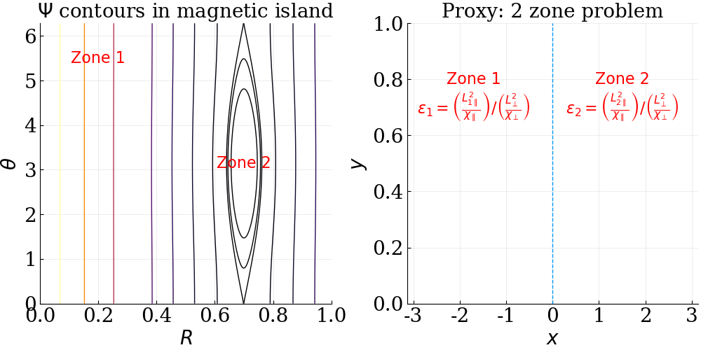
Figure 2: Schematic representation of the unrolling magnetic island into a two-zone configuration. The left figure shows a typical magnetic field topology in cylindrical/toroidal geometry (poloidal angle vs radius). The right figure shows the Cartesian unrolling into a two-zone problem.

A linear analysis (see A) shows that the steady-state solution to the problem for $k_{y}\neq 0$ is

$$T_{s}(x,y)=\chi(x)\sin(k_{y}y),$$ (42)

with

$$\chi(x)=\begin{cases}&-\frac{1}{1+r_{1}^{2}}\sin(x)+A\frac{\sinh\left(r_{1}(x+\pi)\right)}{\sinh\left(r_{1}\pi\right)}\text{, for }x\in[-\pi,0],\\ &A\frac{\sinh\left(r_{2}(\pi-x)\right)}{\sinh\left(r_{2}\pi\right)}\text{, for }x\in(0,\pi],\end{cases}$$ (43)

where $r_{1,2}=k_{y}/\sqrt{\epsilon_{1,2}}$ and

$$A=\frac{1}{1+r_{1}^{2}}\frac{1}{r_{1}\coth\left(\pi r_{1}\right)+r_{2}\coth\left(\pi r_{2}\right)}.$$

The typical shape of the solution along $x$ is plotted in Figure 3. This figure illustrates that the solution mimics the heat source (41) in zone 1, decaying immediately at the beginning of zone 2. This transition region is a boundary layer. Taylor-expanding equation (43) shows that the boundary layer width can be estimated as

$$\delta\approx\frac{1}{r_{2}}=\frac{\sqrt{\epsilon_{2}}}{k_{y}}.$$ (44)

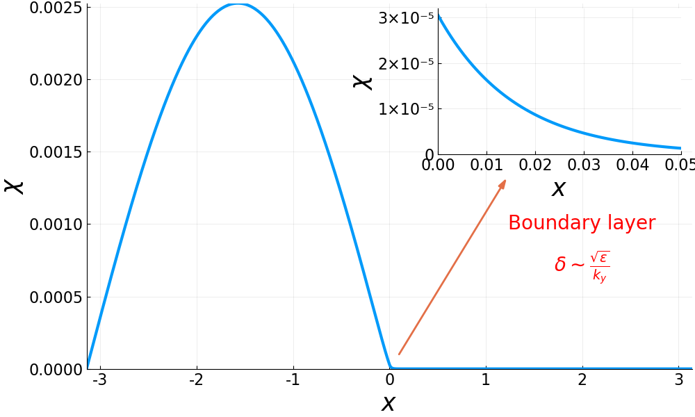
Figure 3: Typical steady state solution (43) and illustration of the boundary layer.

The derivation of the full time-dependent solution for the two-zone problem is described in B. The elliptic nature of the diffusion equation makes the temperature profile relax to the steady-state solution (42),

$$T(t,x,y)=T_{s}(x,y)+\sum_{n=1}^{\infty}C_{n}e^{-\gamma_{n}t}h_{n}(x,y),$$ (45)

where $\gamma_{n}>0$ are real damping rates that can be found from the transcendental dispersion equation in B [Eq. (61)], $h_{n}$ are the eigenfunction of the homogeneous diffusion equation found in B, and $C_{n}=-\langle T_{s},h_{n}\rangle/\langle h_{n},h_{n}\rangle$, with the appropriate integral scalar product $\langle f,g\rangle=\int fgdxdy$, according to the classical Sturm-Liouville theory.

In the first numerical test, we verify that the implicit time discretization can recover the steady-state solution up to spatial discretization errors regardless of the time step. We evolve the simulation for a sufficiently long time $t_{final}=0.04$ to recover the steady-state solution, and vary the time step. We test three time discretization algorithms: BDF1, BDF2, and operator splitting (OP) [18]. We fix the spatial resolution, with the number of points in $x$ to be $N_{x}=64$ and in $y$, $N_{y}=32$. Note that the spatial grid is uniform in $y$, but it is packed in $x$ (i.e., tensor product mesh) around the boundary layer ($x=0$), so the boundary layer is always well resolved. We will relax this later. The actual spatial variation of the mesh size in $x$ direction is shown in Figure 4. Two anisotropy values are chosen for this test, $\epsilon_{1}=10^{-1},\epsilon_{2}=10^{-2}$ and $\epsilon_{1}=10^{-3},\epsilon_{2}=10^{-4}$. We measure the $L_{2}$ error between numerical and analytical steady-state solutions and the results are shown in Figure 5. It is evident form the graph that the operator-split method is first order in time. The steady-state errors in the implicit temporal schemes, however, do not depend on the time step, and the deviation from the analytical solution is only due to spatial error.

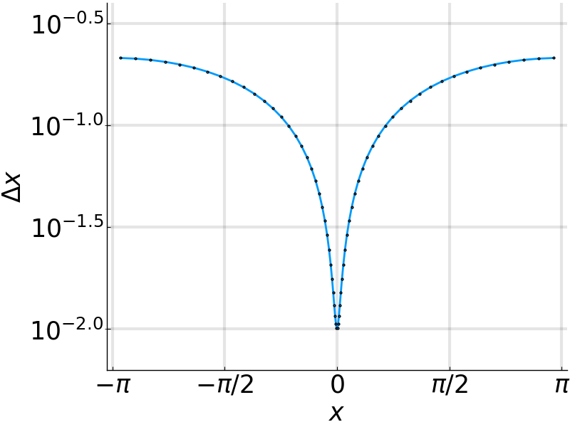
Figure 4: Spatial variation of the mesh size in $x$ direction in two-zone problem.

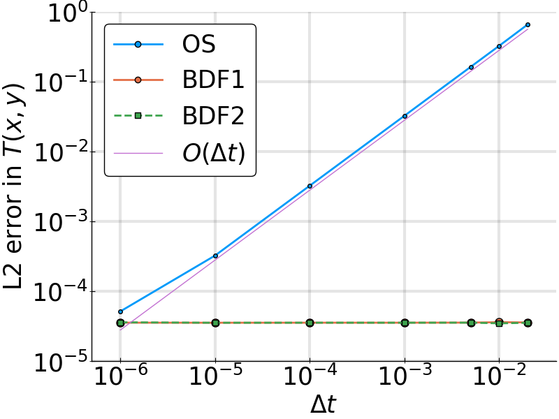
(a) with $\epsilon_{1}=10^{-1},\epsilon_{2}=10^{-2}$

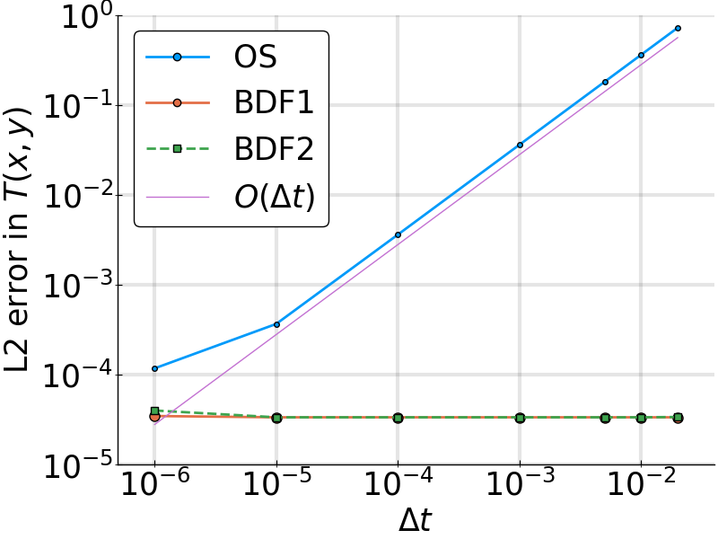
(b) with $\epsilon_{1}=10^{-3},\epsilon_{2}=10^{-4}$

Figure 5: Error in steady-state solution for three different time discretizations: BDF1, BDF2, and operator splitting in two-zone problem versus time step.

Next, we test the time discretization error with the full time-dependent solution. For this test, we modify the initial condition as:

$$T(0,x,y)=T_{s}(x,y)+h_{1}(x,y),$$ (46)

where $h_{1}(x,y)$ is the slowest decaying eigenmode, so the temperature profile evolves exactly as

$$T(t,x,y)=T_{s}(x,y)+e^{-\gamma_{1}t}h_{1}(x,y).$$ (47)

Here, $\gamma_{1}$ is determined by (65) and $h_{1}$ by (62). In this test, we choose the anisotropy ratios $\epsilon_{1}=10^{-1},\epsilon_{2}=10^{-2}$, with corresponding theoretical damping rate $\gamma_{1}^{theory}=395.774$. We measure the experimental damping rate $\gamma_{1}$ by a linear regression of the expression

$$\log\left(\left\|T-T_{s}\right\|_{L_{2}}\right)=-\gamma_{1}t+\log\left(\left\|h_{1}\right\|_{L_{2}}\right),$$

where $\left\|\cdot\right\|_{L_{2}}$ is an $L_{2}$ norm. The results of the relative error in the damping rate are shown in Figure 6, where we can see that BDF1 and OS methods are first-order in time while BDF2 is second-order.

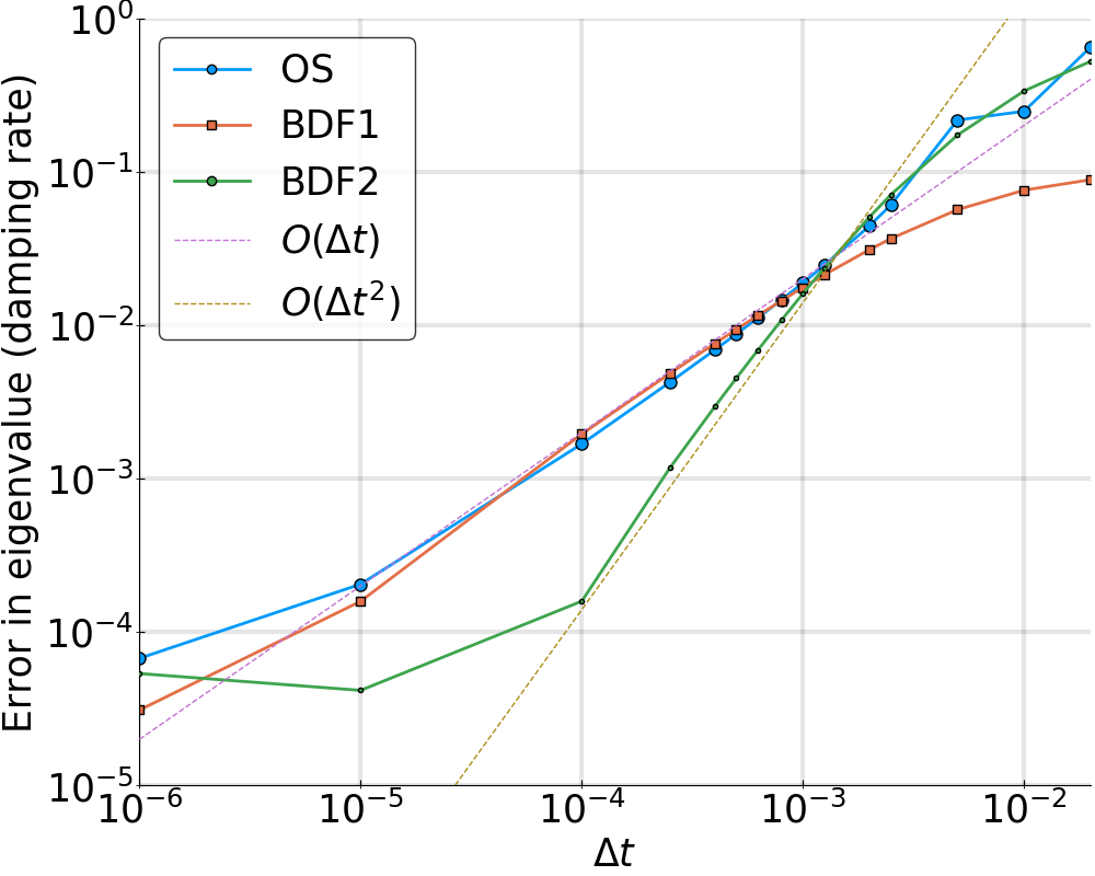
Figure 6: Relative temporal discretization error in the damping rate $\gamma_{1}$ versus time-step of the first eigenfunction $h_{1}$ for three different time discretizations: BDF1, BDF2, and OS in the two-zone problem with $\epsilon_{1}=10^{-1},\epsilon_{2}=10^{-2}$.

Next, we test the numerical error due to the spatial discretization in the steady-state solution. We consider a uniform grid both in $x$ and $y$, and refine the number of spatial points $N_{x}=N_{y}$ (other parameters are left unchanged from the previous test). The results of the $L_{2}$ error are shown in Figure 7. We can see that, when $\Delta x$ is smaller than the boundary layer width Eq. (44), BDF1 and BDF2 are both fourth-order accurate spatially, as expected. However, there is a slight order reduction (less than one order), when the boundary layer is not resolved. The steady-state spatial accuracy is independent of the temporal discretization, also expected.

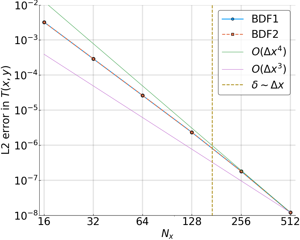
Figure 7: Spatial discretization error in the steady-state solution for BDF1 and BDF2 temporal discretizations in the two-zone problem with $\epsilon_{1}=10^{-1},\epsilon_{2}=10^{-2}$ versus the number of spatial points. The vertical dashed line indicates the width of the boundary layer for this configuration.

8.2 Spatial accuracy test with complex magnetic field topologies and extreme anisotropies ($\chi_{\parallel}/\chi_{\perp}=10^{10}$)

In order to test the spatial accuracy of the semi-Lagrangian formulation with extreme anisotropies, we consider a 2D domain with $L_{x}=L_{y}=1$ and homogeneous Dirichlet boundary conditions in $x$ and periodic boundary conditions in $y$. We consider a steady-state manufactured solution of the form $T_{\infty}(x,y)=\psi(x,y)$, with $\psi$ the poloidal flux given by

$$\psi=x+\delta\sin(2\pi x)\cos(2\pi y),$$ (48)

with $\delta=1/2$ (for which $\psi$ features several magnetic islands; see Figure 8-left). The magnetic field is given by $\mathbf{B}=\mathbf{z}\times\nabla\Psi+B_{z}\mathbf{z}$, with $B_{z}=1$. With these choices, $T_{\infty}(x,y)$ is in the kernel of the parallel transport operator, i.e., $\nabla_{\parallel}^{2}T_{\infty}=0$. This is similar to other tests proposed in the literature [7], and is designed to allow a clean measurement of numerical error pollution by the stiff parallel transport dynamics. The source $S(\mathbf{x})$ in Equation (8.2) that drives the temperature field to this steady-state solution is found as:

$$S(x,y)=-\nabla_{\perp}^{2}T_{\infty}=-\nabla^{2}\psi=4\pi^{2}\sin(2\pi x)\cos(2\pi y).$$

The results of the convergence study in Figure 8-right demonstrate spatial convergence close to or at design accuracy for both second- and fourth-order discretizations, with relative errors small even for very coarse meshes. This confirms the ability of the scheme to capture null-space components of the solution accurately, without pollution from the parallel-transport dynamics.

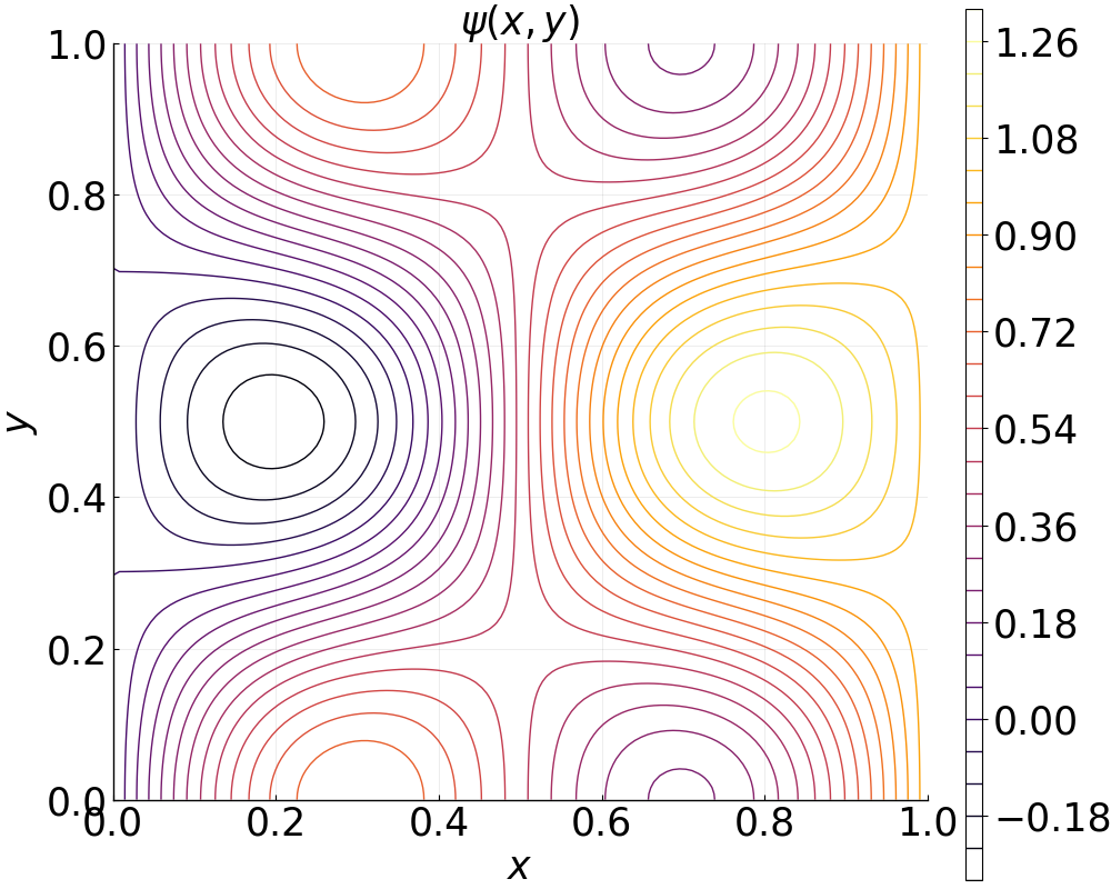
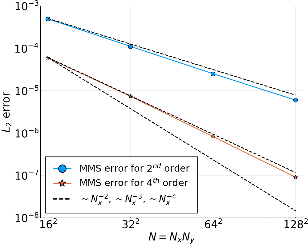
Figure 8: Left: Poloidal flux for manufactured solution test with extreme anisotropy. Right: Scaling of spatial error in steady state with respect to the manufactured solution $T_{\infty}$ for $\chi_{\parallel}/\chi_{\perp}=10^{10}$, demonstrating desing accuracy for the second-order discretization, and convergence between third and fourth order for our fourth-order implementation. Error is measured with an $L_{2}$-norm with respect to the analytical steady state, and is normalized to the maximum temperature value.

8.3 Performance tests

We assess next the performance of the preconditioner proposed in Section 6 for both trivial ($\delta=0.1$) and complex ($\delta=0.5$) magnetic field topologies with extreme anisotropy, $\chi_{\parallel}/\chi_{\perp}=10^{10}$. For this test, we use the second-order discretization of the isotropic Laplacian operator.

A convergence study for a GMRES tolerance of $\epsilon_{r}=10^{-3}$ is presented in Table 1 for the same setup as in Section 8.2 for two values of the parameter $\delta$ (0.1 and 0.5), and for various mesh sizes and timesteps. For $\delta=0.1$, the magnetic field is simply connected, and no boundary layers exist (not shown). The Table demonstrates no dependence of the convergence rate with mesh refinement, and very weak dependence on the timestep, as expected from the discussion in Sec. 6.

For $\delta=0.5$, the magnetic field topology features islands, and therefore boundary layers. Accordingly, off-null-space components will be present in the solution to enforce continuity of the temperature field across these boundary layers. This manifests in the results in the Table, where sensitivity to both resolution and timestep can be observed. However, there is a marked transition in performance between $\Delta t=0.01$ and $\Delta t=0.1$. Below $\Delta t=0.01$, the convergence rate of the scales as $\sim(N\Delta t)^{1/4}$. Above $\Delta t=0.1$, the convergence rate becomes largely independent of mesh refinement and improves with larger $\Delta t$ (both a consequence of improved eigenvalue clustering). For this problem, the $\beta_{\mathrm{min}}=4\pi^{2}\chi_{\perp}\Delta t/L^{2}>1$ threshold advanced in Sec. 6 corresponds to $\Delta t>L^{2}/(4\pi^{2}\chi_{\perp})\approx 0.025$, which fully explains the transition in convergence behavior. When the residual is analyzed during the course of the iteration for $\Delta t<0.025$, the error is seen to concentrate around the island separatrices (not shown), suggesting that convergence is hampered by the presence of off-null-space components. The unpreconditioned case recovers the standard dependence of the Krylov convergence rate with mesh size and timestep, $\sqrt{N\Delta t}$ for all timesteps considered, demonstrating the effectiveness of the preconditioner in decreasing the iteration count.

Table 1: Convergence study for various mesh sizes and timesteps for $\chi_{\parallel}/\chi_{\perp}=10^{10}$ and $\delta=0.1$, 0.5 with the second-order discretization. Timesteps considered $\Delta t=10^{-5},0.001,0.01,0.1,1.0$. Note that the first timestep is the accuracy limit for the operator-split algorithm in Ref. [18] ($\Delta t=\sqrt{\frac{\chi_{\perp}}{\chi_{\parallel}}}$). The numbers indicated by “id” indicate unpreconditioned GMRES iterations.

	$\Delta t=10^{-5}$		$\Delta t=0.001$		$\Delta t=0.01$		$\Delta t=0.1$		$\Delta t=1.0$
Mesh/$\delta$	$0.1$	$0.5$	$0.1$	$0.5$	$0.1$	$0.5$	$0.1$	$0.5$	$0.1$	$0.5$
$32\times 32$	1	2	4	9 (id=9)	8	22 (id=24)	10	20 (id=51)	14	16
$64\times 64$	1	2	4	15 (id=16)	8	36 (id=45)	6	22 (id=83)	10	13
$128\times 128$	1	4	5	23 (id=30)	8	46 (id=84)	5	21 (id=111)	4	17
$256\times 256$	1	5	5	37 (id=62)	8	63 (id=196)	5	19 (id=269)	3	14

9 Discussion

We have developed and implemented a new preconditioned implicit solver for the semi-Lagrangian asymptotically preserving scheme for the strongly anisotropic heat transport equation proposed in [18]. The implicit algorithm is demonstrated to be much more accurate than the operator-split one proposed in the reference, both for steady-state solutions as well as solutions with boundary layers.

GMRES solver performance is independent of the anisotropy ratio, which is critical. We have proposed a simple preconditioner that results in the number of GMRES iterations $N_{i}$ scaling as $(N\Delta t)^{1/4}$, with $N$ the total number of mesh points. Since our equations are normalized to the perpendicular transport time scale, $\tau_{\perp}=L_{\perp}^{2}/\chi_{\perp}$, and $N=(L/\Delta)^{2}$, with $\Delta$ the mesh spacing, one can rewrite this result as $N_{i}\sim\left(\frac{\Delta t}{\tau_{\perp}}\right)^{1/4}\sqrt{\frac{L_{\perp}}{\Delta}}$.

While in principle the method does not scale optimally under mesh and time-step refinement, it is still instructive to compare its computational performance vs the operator-split one of Ref. [18]. We can estimate the computational cost of the operator splitting method as:

$$\mbox{CPU time}\sim\frac{T^{final}}{\Delta t_{OS}}\sim\frac{T^{final}}{\tau_{\perp}\sqrt{\chi_{\perp}/\chi_{\parallel}}},$$ (49)

where the time step restriction $\Delta t_{OS}\sim\tau_{\perp}\sqrt{\chi_{\perp}/\chi_{\parallel}}$ is needed to avoid $O(1)$ errors at boundary layers (e.g., at magnetic island separatrices). At the same time, the cost of the implicit method is:

$$\mbox{CPU time}\sim\frac{T^{final}N_{i}}{\Delta t}.$$ (50)

The speed-up can therefore be estimated as:

$$\mbox{speedup}=\frac{\left(\mbox{CPU time}\right)_{OS}}{\left(\mbox{CPU time}\right)_{impl}}\sim\sqrt{\frac{\Delta}{L_{\perp}}}\left(\frac{\Delta t}{\tau_{\perp}}\right)^{3/4}\sqrt{\frac{\chi_{\parallel}}{\chi_{\perp}}}.$$ (51)

This expression implies that the implicit method favors large time steps and high anisotropy, and in this regime it is significantly more efficient than the operator-split approach.

Finally, it is worth noting that, in many practical applications of interest (and in particular for magnetic thermonuclear fusion) for which $\chi_{\perp}$ is very small, time and mesh resolution requirements compatible with other physical processes (e.g. magnetohydrodynamics) satisfy $\Delta t\sim\tau_{\perp}$ and $\Delta\sim L_{\perp}$, thus leading to $N_{i}\sim\mathcal{O}(1)$ and making the algorithm competitive in practice.

10 Conclusion

In this study, we have investigated the merits and capabilities of a new fully implicit, asymptotic-preserving, semi-Lagrangian algorithm for the time-dependent anisotropic heat-transport equation. The new method is an implicit extension of the operator-split approach proposed in [18]. The integro-differential formulation of the parallel transport operator is the key element to ensure asymptotically preserving properties in the limit of arbitrary anisotropy, thereby avoiding numerical pollution. The perpendicular transport is treated as a formal source to the purely parallel transport equation, thus constituting an implicit integro-differential equation. The resulting linear system is inverted with GMRES, and preconditioned to be compact. For complex magnetic-field topologies and below a timestep size threshold, the preconditioner results in Krylov convergence in $N_{i}\sim(N\Delta t)^{1/4}$ iterations, i.e., scaling very weakly with mesh refinement and time-step size and independently of the anisotropy ratio $\epsilon$. Above the timestep threshold, convergence is essentially mesh- and timestep-independent. Additionally, the new implicit formulation is unconditionally stable and preserves the positivity of the solution for physical initial conditions.

Similarly to the operator-split formulation, the implicit version can handle complicated magnetic field topologies and very large anisotropy ratios without introducing numerical pollution. However, unlike the operator-split approach, its implicit nature ensures accurate steady states regardless of $\Delta t$, and can be readily made higher-order temporally (e.g., BDF2). The implicit formulation favors large time steps and high anisotropy, with speedups vs. the operator-split approach $\sim\Delta t^{3/4}\sqrt{\chi_{\parallel}/\chi_{\perp}}$.

The proposed approach features a number of simplifications that make it unsuitable for some class of problems. The main two limitations are the approximation $\nabla\cdot\mathbf{b}\approx 0$ (for which we have devised a solution that will be documented in a future publication) and the assumption of constant parallel conductivity along field lines (arbitrary variations of $\chi_{\perp}$ and variation of $\chi_{\parallel}$ across field lines can be handled with the current formulation of the method). The extension of the method to remove the latter limitation will be considered in the future.

Appendix A Steady-state solution to the two-zone problem

In order to derive the steady-state solution (42), we look for a solution of the form $T=\chi(x)\sin(k_{y}y)$, such that:

$$\chi^{\prime\prime}_{1}-\frac{k_{y}^{2}}{\epsilon_{1}}\chi_{1}=\sin(x),$$ (52)

$$\chi^{\prime\prime}_{2}-\frac{k_{y}^{2}}{\epsilon_{2}}\chi_{2}=0,$$ (53)

where indices $1$ and $2$ correspond to zone 1 ($x\in[-\pi,0]$) and 2 ($x\in[0,\pi]$), respectively. The solution which satisfies the boundary conditions

$$\chi_{1}(-\pi)=\chi_{2}(\pi)=0,\quad\chi_{1}(0)=\chi_{2}(0),\quad\chi_{1}^{\prime}(0)=\chi_{2}^{\prime}(0),$$

is:

$$\chi_{1}(x)=-\frac{1}{1+r_{1}^{2}}\sin(x)+A\frac{\sinh\left(r_{1}(x+\pi)\right)}{\sinh\left(r_{1}\pi\right)},$$ (54)

$$\chi_{2}(x)=A\frac{\sinh\left(r_{2}(\pi-x)\right)}{\sinh\left(r_{2}\pi\right)},$$ (55)

where $r_{1,2}=k_{y}/\sqrt{\epsilon_{1,2}}$ and

$$A=\frac{1}{1+r_{1}^{2}}\frac{1}{r_{1}\coth\left(\pi r_{1}\right)+r_{2}\coth\left(\pi r_{2}\right)},$$

which is (43).

Appendix B Time-dependent solution of the two-zone problem

In this section, we extend the analysis of A to include the time evolution of the solution. Since the steady-state solution is already known and the equation (1) is linear, it is sufficient to solve the homogeneous equation

$$\partial_{t}T-\frac{1}{\epsilon}\partial_{y}^{2}T-\partial_{x}^{2}T=0,$$ (56)

with $\epsilon$, boundary conditions defined in Sections 8.1, and initial condition $T(0,x,y)=-T_{s}(x,y)$ where $T_{s}$ is the steady-state solution from A (note that the initial condition of the initial problem is zero).

Separation of variables $T=\tau(t)X(x)\sin(k_{y}y)$ (with $k_{y}\neq 0$) leads to

$$\tau(t)=\tau(0)e^{-\gamma t},$$ (57)

where eigenvalues $\gamma$ (damping rates) and eigenfunctions $X(x)$ are determined from the boundary value problem (note the discontinuity in $\epsilon$)

$$X^{\prime\prime}-\left(\frac{k_{y}^{2}}{\epsilon}-\gamma\right)X=0,$$ (58)

$$X(-\pi)=X(\pi)=0.$$ (59)

After some algebra, the boundary value problem solution yield

$$X(x)=\begin{cases}&\frac{\sin(\sigma_{1}(\pi+x))}{\sin(\pi\sigma_{1})}\text{, for }x\leq 0,\\ &\frac{\sinh(\lambda_{2}(\pi-x))}{\sinh(\pi\lambda_{2})}\text{, for }x\geq 0,\end{cases}$$ (60)

with $\sigma_{1}=\sqrt{\gamma-r_{1}^{2}}$, and $\lambda_{2}=\sqrt{r_{2}^{2}-\gamma}$ (we also define $\lambda_{1}=\sqrt{r_{1}^{2}-\gamma}$, and $\sigma_{2}=\sqrt{\gamma-r_{2}^{2}}$ ) where $\gamma$ is a solution to the dispersion equation

$$\frac{\tan(\pi\sigma_{1})}{\pi\sigma_{1}}+\frac{\tanh(\pi\lambda_{2})}{\pi\lambda_{2}}=0.$$ (61)

Using the eigenmodes obtained from the boundary value problem, we derive the solution of the homogeneous system (56)

$$T=\sin(k_{y}y)\sum_{n}C_{n}e^{-\gamma_{n}t}\begin{cases}&\frac{\sin(\sigma_{1}^{n}(\pi+x))}{\sin(\pi\sigma_{1}^{n})}\text{, for }x\leq 0,\\ &\frac{\sinh(\lambda_{2}^{n}(\pi-x))}{\sinh(\pi\lambda_{2}^{n})}\text{, for }x\geq 0,\end{cases}$$ (62)

where summation is performed over all eigenmodes and corresponding eigenvalues $\gamma^{n}$ (and $\sigma_{1}^{n}$, $\lambda_{2}^{n}$) found from the dispersion equation (61). The coefficient $C_{n}$ should be computed from the initial condition expanded in a basis of eigenfunctions found from the boundary value problem.

It is impossible to solve the dispersion equation (61) analytically. However, it is possible to estimate the smallest growth rate for the parameters of interest. First, we notice that there are no roots for $\mbox{Im}[\lambda_{1}]=\mbox{Im}[\lambda_{2}]=0$, thus the smallest $\gamma$ will appear in the regime

$$\frac{k_{y}^{2}}{\epsilon_{1}}<\gamma<\frac{k_{y}^{2}}{\epsilon_{2}},$$ (63)

when $\sigma_{1},\lambda_{2}$ are real. Note that the dispersion equation (61) is written with this assumption in mind, since all eigenvalues $\gamma$ must be real. First roots (ordering in increasing order) of the dispersion equation in the regime when $\epsilon_{1}\gg\epsilon_{2}$ will appear in the intersection with the flat part of the hyperbolic tangent curve, which can be very well approximated by a constant:

$$\frac{\tanh(\pi\kappa_{2})}{\pi\kappa_{2}}\sim\frac{\tanh(\pi k_{y}/\sqrt{\epsilon_{2}})}{\pi k_{y}/\sqrt{\epsilon_{2}}},$$

with $\tan(x)/x$ branches on intervals $(\pi/2+\pi n,3\pi/2+\pi n)$ for $n=1,2,\dots$. The tangent term can be approximated linearly as

$$\frac{\tan(\pi\sigma_{1})}{\pi\sigma_{1}}\sim\frac{\sigma_{1}-n}{n},$$

which leads to the eigenvalue estimates

$$\gamma_{n}=\frac{k_{y}^{2}}{\epsilon_{1}}+n^{2}\left(1-\frac{\tanh(\pi k_{y}/\sqrt{\epsilon_{2}})}{\pi k_{y}/\sqrt{\epsilon_{2}}}\right)^{2}.$$ (64)

Note that, for all parameters of interest, $\xi=\pi k_{y}/\sqrt{\epsilon}\gg 1$ and $\tanh(\xi)/\xi\ll 1$, thus eigenvalues grow quickly as $n^{2}$. Therefore, the less damped and most important eigenvalue which controls the time evolution most of the time (except perhaps during the initial transient phase) is

$$\gamma=\gamma_{1}=\frac{k_{y}^{2}}{\epsilon_{1}}+\left(1-\frac{\tanh(\pi k_{y}/\sqrt{\epsilon_{2}})}{\pi k_{y}/\sqrt{\epsilon_{2}}}\right)^{2}.$$ (65)

Appendix C Performing the Fourier kernel integral

In this section, we simplify the expression of the Fourier kernel $\mathcal{K}(\mathbf{x})$ in (28). First, we use the fact that

$$\int d^{2}k_{\perp}\frac{e^{i\mathbf{k}_{\perp}\cdot\mathbf{x}_{\perp}}}{1+ak_{\perp}^{2}}=2\pi\int_{0}^{\infty}dk_{\perp}\frac{k_{\perp}}{1+ak_{\perp}^{2}}\frac{1}{\pi}\int_{0}^{\pi}d\theta e^{ik_{\perp}r_{\perp}\cos\theta}=$$ (66)

$$= 2\pi\int_{0}^{\infty}dk_{\perp}\frac{k_{\perp}}{1+ak_{\perp}^{2}}J_{0}(k_{\perp}r_{\perp})=\frac{2\pi}{a}K_{0}\left(\frac{r_{\perp}}{\sqrt{a}}\right),$$ (67)

where $a>0$ is a positive constant, $r_{\perp}=|\mathbf{x}_{\perp}|$, $J_{0},K_{0}$ are the first-kind and modified second-kind Bessel functions, respectively. The last step in the integration used equation (11.4.44) on p488 in [34]. Now we apply it to the kernel integral:

$$\mathcal{K}(\mathbf{x})=\frac{1}{(2\pi)^{3}}\text{Re}\left[\int d^{3}ke^{i\mathbf{k}\cdot\mathbf{x}}\frac{e^{-\alpha}}{1+\beta(\frac{1-e^{-\alpha}}{\alpha})}\right],$$ (68)

with $\beta=\Delta tk_{\perp}^{2}$ and get:

$$\mathcal{K}(\mathbf{x})=\frac{1}{4\pi^{2}\Delta t}\int_{-\infty}^{\infty}dk_{\parallel}\cos(k_{\parallel}z)e^{-\alpha}\frac{\alpha}{1-e^{-\alpha}}K_{0}\left(r_{\perp}\sqrt{\frac{\alpha}{1-e^{-\alpha}}}\right).$$ (69)

References

- Braginskii [1963] S. Braginskii, Transport phenomena in plasma, Reviews of plasma physics 1 (1963) 205.
- Hölzl et al. [2009] M. Hölzl, S. Günter, I. Classen, Q. Yu, E. Delabie, T. Team, et al., Determination of the heat diffusion anisotropy by comparing measured and simulated electron temperature profiles across magnetic islands, Nuclear fusion 49 (2009) 115009.
- Ren et al. [1998] C. Ren, J. D. Callen, T. A. Gianakon, C. C. Hegna, Z. Chang, E. D. Fredrickson, K. M. McGuire, G. Taylor, M. C. Zarnstorff, Measuring ’ from electron temperature fluctuations in the Tokamak Fusion Test Reactor, Physics of Plasmas 5 (1998) 450–454.
- Meskat et al. [2001] J. Meskat, H. Zohm, G. Gantenbein, S. Günter, M. Maraschek, W. Suttrop, Q. Yu, A. U. Team, Analysis of the structure of neoclassical tearing modes in ASDEX Upgrade, Plasma Physics and Controlled Fusion 43 (2001) 1325.
- Snape et al. [2012] J. Snape, K. Gibson, T. O’gorman, N. Barratt, K. Imada, H. Wilson, G. Tallents, I. Chapman, et al., The influence of finite radial transport on the structure and evolution of m/n= 2/1 neoclassical tearing modes on MAST, Plasma Physics and Controlled Fusion 54 (2012) 085001.
- Choi et al. [2014] M. J. Choi, G. S. Yun, W. Lee, H. K. Park, Y.-S. Park, S. A. Sabbagh, K. J. Gibson, C. Bowman, C. W. Domier, N. C. Luhmann Jr, et al., Improved accuracy in the estimation of the tearing mode stability parameters (’ and ) using 2D ECEI data in KSTAR, Nuclear Fusion 54 (2014) 083010.
- Sovinec et al. [2004] C. Sovinec, A. Glasser, T. Gianakon, D. Barnes, R. Nebel, S. Kruger, D. Schnack, S. Plimpton, A. Tarditi, M. Chu, et al., Nonlinear magnetohydrodynamics simulation using high-order finite elements, Journal of Computational Physics 195 (2004) 355–386.
- Günter et al. [2005] S. Günter, Q. Yu, J. Krüger, K. Lackner, Modelling of heat transport in magnetised plasmas using non-aligned coordinates, Journal of Computational Physics 209 (2005) 354–370.
- Günter et al. [2007] S. Günter, K. Lackner, C. Tichmann, Finite element and higher order difference formulations for modelling heat transport in magnetised plasmas, Journal of Computational Physics 226 (2007) 2306–2316.
- Günter and Lackner [2009] S. Günter, K. Lackner, A mixed implicit–explicit finite difference scheme for heat transport in magnetised plasmas, Journal of Computational Physics 228 (2009) 282–293.
- Sharma and Hammett [2007] P. Sharma, G. W. Hammett, Preserving monotonicity in anisotropic diffusion, Journal of Computational Physics 227 (2007) 123–142.
- Kuzmin et al. [2009] D. Kuzmin, M. J. Shashkov, D. Svyatskiy, A constrained finite element method satisfying the discrete maximum principle for anisotropic diffusion problems, Journal of Computational Physics 228 (2009) 3448–3463.
- Du Toit et al. [2018] E. J. Du Toit, M. R. O’Brien, R. G. Vann, Positivity-preserving scheme for two-dimensional advection–diffusion equations including mixed derivatives, Computer Physics Communications 228 (2018) 61–68.
- Held et al. [2001] E. Held, J. Callen, C. Hegna, C. Sovinec, Conductive electron heat flow along magnetic field lines, Physics of Plasmas 8 (2001) 1171–1179.
- Held et al. [2004] E. Held, J. Callen, C. Hegna, C. Sovinec, T. Gianakon, S. Kruger, Nonlocal closures for plasma fluid simulations, Physics of Plasmas 11 (2004) 2419–2426.
- del Castillo-Negrete and Chacón [2011] D. del Castillo-Negrete, L. Chacón, Local and nonlocal parallel heat transport in general magnetic fields, Physical review letters 106 (2011) 195004.
- del Castillo-Negrete and Chacón [2012] D. del Castillo-Negrete, L. Chacón, Parallel heat transport in integrable and chaotic magnetic fields, Physics of Plasmas 19 (2012) 056112.
- Chacón et al. [2014] L. Chacón, D. del Castillo-Negrete, C. D. Hauck, An asymptotic-preserving semi-lagrangian algorithm for the time-dependent anisotropic heat transport equation, Journal of Computational Physics 272 (2014) 719–746.
- Larsen et al. [1987] E. W. Larsen, J. E. Morel, W. F. Miller Jr, Asymptotic solutions of numerical transport problems in optically thick, diffusive regimes, Journal of Computational Physics 69 (1987) 283–324.
- Larsen and Morel [1989] E. W. Larsen, J. E. Morel, Asymptotic solutions of numerical transport problems in optically thick, diffusive regimes II, Journal of Computational Physics (1989).
- Jin [1999] S. Jin, Efficient asymptotic-preserving (AP) schemes for some multiscale kinetic equations, SIAM Journal on Scientific Computing 21 (1999) 441–454.
- Saad and Schultz [1986] Y. Saad, M. H. Schultz, GMRES: A generalized minimal residual algorithm for solving nonsymmetric linear systems, SIAM Journal on scientific and statistical computing 7 (1986) 856–869.
- Degond et al. [2012] P. Degond, F. Deluzet, A. Lozinski, J. Narski, C. Negulescu, Duality-based asymptotic-preserving method for highly anisotropic diffusion equations, Communications in Mathematical Sciences 10 (2012) 1–31.
- Degond et al. [2010] P. Degond, F. Deluzet, C. Negulescu, An asymptotic preserving scheme for strongly anisotropic elliptic problems, Multiscale Modeling & Simulation 8 (2010) 645–666.
- Degond et al. [2012] P. Degond, A. Lozinski, J. Narski, C. Negulescu, An asymptotic-preserving method for highly anisotropic elliptic equations based on a micro–macro decomposition, Journal of Computational Physics 231 (2012) 2724–2740.
- Narski and Ottaviani [2014] J. Narski, M. Ottaviani, Asymptotic preserving scheme for strongly anisotropic parabolic equations for arbitrary anisotropy direction, Computer Physics Communications 185 (2014) 3189–3203.
- Wang et al. [2018] Y. Wang, W. Ying, M. Tang, Uniformly convergent scheme for strongly anisotropic diffusion equations with closed field lines, SIAM Journal on Scientific Computing 40 (2018) B1253–B1276.
- Daniel [1967] J. W. Daniel, The conjugate gradient method for linear and nonlinear operator equations, SIAM Journal on Numerical Analysis 4 (1967) 10–26.
- Campbell et al. [1996a] S. L. Campbell, I. C. Ipsen, C. T. Kelley, C. Meyer, Z. Xue, Convergence estimates for solution of integral equations with GMRES, The Journal of Integral Equations and Applications (1996a) 19–34.
- Campbell et al. [1996b] S. L. Campbell, I. C. Ipsen, C. T. Kelley, C. D. Meyer, Gmres and the minimal polynomial, BIT Numerical Mathematics 36 (1996b) 664–675.
- Rasmussen [2001] J. M. Rasmussen, Compact linear operators and Krylov subspace methods, Citeseer, 2001.
- Hindmarsh [1983] A. C. Hindmarsh, ODEPACK, a systematized collection of ODE solvers, Scientific computing (1983) 55–64.
- Chacon et al. [2022] L. Chacon, D. Daniel, W. T. Taitano, An asymptotic-preserving 2d-2p relativistic drift-kinetic-equation solver for runaway electron simulations in axisymmetric tokamaks, Journal of Computational Physics 449 (2022) 110772.
- Abramowitz and Stegun [1964] M. Abramowitz, I. Stegun, Handbook of mathematical functions: With formulas, graphs, and mathematical tables applied mathematics series, National Bureau of Standards, Washington, DC (1964) 295–300.