Leveraging Normalizing Flows for Orbital-Free Density Functional Theory

Abstract

Orbital-free density functional theory (OF-DFT) for real-space systems has historically depended on Lagrange optimization techniques, primarily due to the inability of previously proposed electron density ansatze to ensure the normalization constraint. This study illustrates how leveraging contemporary generative models, notably normalizing flows (NFs), can surmount this challenge. We pioneer a Lagrangian-free optimization framework by employing these machine learning models as ansatze for the electron density. This novel approach also integrates cutting-edge variational inference techniques and equivariant deep learning models, offering an innovative alternative to the OF-DFT problem. We demonstrate the versatility of our framework by simulating a one-dimensional diatomic system, LiH, and comprehensive simulations of H₂, LiH, and H₂O molecules. The inherent flexibility of NFs facilitates initialization with promolecular densities, markedly enhancing the efficiency of the optimization process.

Mc]Department of Chemistry and Chemical Biology, McMaster University, Hamilton, ON, Canada meta]FAIR at Meta, NY, USA Mc]Department of Chemistry and Chemical Biology, McMaster University, Hamilton, ON, Canada [BIMR]Brockhouse Institute for Materials Research, McMaster University, Hamilton, ON, Canada ML, OF-DFT, Normalizing Flows

Introduction: The Density Functional Theory (DFT) framework has evolved into an indispensable tool in both computational materials science and chemistry, with the Kohn-Sham (KS) formalism being the de facto (or most commonly employed) form of DFT ¹, ², ³, ⁴. The success of the KS formalism sparked a race to develop exchange-correlation (XC) energy functionals based on electronic spin densities ⁵, ⁶, ⁷, ⁸, ⁹, ¹⁰, ¹¹. Initially, physics-motivated functionals were the predominant framework until machine learning (ML) approaches emerged, marking a noteworthy shift in the landscape of quantum chemistry ¹², ¹³, ¹⁴, ¹⁵, ¹⁶, ¹⁷.

Given its computational scaling, orbital-free DFT (OF-DFT), rooted in the Hohenberg-Kohn theorems ¹⁸, ¹⁹, is a promising alternative to KS-DFT. However, the imperative for relative accuracy in kinetic energy (KE) functionals, comparable to the total energy, remains a primary impediment ²⁰. Research endeavors have extensively explored the parametrization of KE functionals ²¹, ²², ²³, surpassing the original Thomas-Fermi-Weizäcker-based formulation. Notable extensions involve non-local KE functionals based on linear response theory, such as the Wang-Teter ²⁴, Perrot ²⁵, Wang-Govind-Carter ²⁶, Huang-Carter ²⁷, Smargiassi-Madden ²⁸, Foley-Madden  ²⁹ and Mi-Genova-Pavanello ³⁰ functionals, showcasing the capability of OF-DFT in simulating systems with a large number of atoms.

Similar to the development of XC functionals, the pursuit of highly accurate OF-DFT simulations has driven the development of KE functionals through ML algorithms. Predominant approaches employ Kernel Ridge Regression ³¹, convolutional neural networks ³², and ResNets ³³. Notably, data used for training ML-based KE functionals are generated through KS-based simulations. However, a key limitation in data-driven functionals lies in the accuracy of functional derivatives, which, when poor, can result in highly inaccurate densities. Despite significant recent progress in materials modeling within the OF-DFT framework, which now includes ML technologies, a consistent aspect for real-space simulations has been the parametrized form of the trial electron density. These traditional approaches have forced the OF-DFT framework to be a Lagrangian-based scheme. In this work, we propose a novel approach employing generative models, specifically normalizing flows, circumventing the normalization constraints that affect traditional methods in the OF-DFT real-space setup.

Methods: In the OF-DFT framework, the ground state energy ($E_{\text{gs}}$) and electron density ($\operatorname{\rho_{{\cal M}}}$) are determined by minimizing the total energy functional ($E[\operatorname{\rho_{{\cal M}}}]$),

$$\begin{split}E_{\text{gs}}&=\inf_{\operatorname{\rho_{{\cal M}}}\in\Omega}E[\operatorname{\rho_{{\cal M}}}(\operatorname{\boldsymbol{x}})],\\ \Omega&=\left\{\operatorname{\rho_{{\cal M}}}:\operatorname{\rho_{{\cal M}}}\in X,\int\operatorname{\rho_{{\cal M}}}(\operatorname{\boldsymbol{x}})\mathrm{d}\operatorname{\boldsymbol{x}}=\operatorname{N_{e}}\right\},\end{split}$$ (1)

where the admissible class of ansatz ($X$) for $\operatorname{\rho_{{\cal M}}}$ must satisfy the normalization constraint on the total number of particles $\operatorname{N_{e}}$. The OF-DFT framework’s resemblance to variational inference in machine learning ³⁴ lies in their shared objective of approximating/learning a density distribution through an optimization/minimization procedure. All previously proposed/developed ansatz belong to the category of density models known as “energy-based models” ³⁵. For instance, $\operatorname{\rho_{{\cal M}}}=f^{2}_{\phi}(\operatorname{\boldsymbol{x}})/\int f^{2}_{\phi}(\operatorname{\boldsymbol{x}})\mathrm{d}\operatorname{\boldsymbol{x}}$ or $\operatorname{\rho_{{\cal M}}}=e^{-f_{\phi}(\operatorname{\boldsymbol{x}})}/\int e^{-f_{\phi}(\operatorname{\boldsymbol{x}})}\mathrm{d}\operatorname{\boldsymbol{x}}$. Common approaches for $f_{\phi}$ include multi-grid ³⁶ and wavelet frameworks ³⁷, as well as a linear combination of atomic Gaussian basis sets ³⁸. Although these frameworks are robust, they require the inclusion of a Lagrange multiplier $\mu$ in the minimization protocols, associated with the normalization constraint on $\operatorname{N_{e}}$, also referred to as the chemical potential.

$$\min_{\operatorname{\rho_{{\cal M}}}}E[\operatorname{\rho_{{\cal M}}}(\operatorname{\boldsymbol{x}})]-\mu\left(\int\operatorname{\rho_{{\cal M}}}(\operatorname{\boldsymbol{x}})\mathrm{d}\operatorname{\boldsymbol{x}}-\operatorname{N_{e}}\right).$$ (2)

Typically, conventional methods for solving for $\operatorname{\rho_{{\cal M}}}$ in real space involve self-consistent procedures based on functional derivatives, resulting in the Euler–Lagrange equation $\delta E[\operatorname{\rho_{{\cal M}}}(\operatorname{\boldsymbol{x}})]/\delta\operatorname{\rho_{{\cal M}}}(\operatorname{\boldsymbol{x}})-\mu=0$ ¹⁹.

In this work, we introduce an alternative ansatz for parameterizing $\operatorname{\rho_{{\cal M}}}$ using normalizing flows (NFs), denoted as $\operatorname{\rho_{\phi}}$ (Eq. 4). We define $\operatorname{\rho_{{\cal M}}}$ as,

$$\operatorname{\rho_{{\cal M}}}(\operatorname{\boldsymbol{x}}):=\operatorname{N_{e}}\operatorname{\rho_{\phi}}(\operatorname{\boldsymbol{x}}),$$ (3)

ensuring the satisfaction of the normalization constraint. The term $\operatorname{\rho_{\phi}}$ is also referred to as the shape factor ¹⁹, ³⁹. This NF-based ansatz allows us to reframe the OF-DFT variational problem as a Lagrangian-free optimization problem for molecular densities in real space, as the normalization is guaranteed regardless of the changes of $\operatorname{\rho_{\phi}}$.

NFs are deep generative models capable of transforming a base (simple) density distribution $\operatorname{\rho_{0}}$ into a target (complex) density distribution ($\rho_{\phi}$) by leveraging the change of variables formula (Fig. 1),

$$\operatorname{\rho_{\phi}}(\mathbf{x})=\operatorname{\rho_{0}}(\mathbf{z})\left|\text{det}\nabla_{\operatorname{\mathbf{z}}}\operatorname{T_{\phi}}(\operatorname{\mathbf{z}})\right|^{-1},$$ (4)

where $\operatorname{T_{\phi}}$ is a bijective transformation. Eq. (4) guarantees the preservation of volume in the density transformation, while also allowing the computation of the target density in a tractable manner, making NFs a promising candidate for parameterizing $\operatorname{\rho_{{\cal M}}}$. Additionally, automatic differentiation tools allow the computation of high-order gradients of $\operatorname{\rho_{{\cal M}}}$, commonly required in density functionals.

The proposed framework is rooted in optimal transport and measure theory where $\operatorname{\rho_{\phi}}$ is known as the push-forward of $\operatorname{\rho_{0}}$ by the function $\operatorname{T_{\phi}}$, denoted by $\operatorname{\rho_{\phi}}=\operatorname{T_{\phi}}\star\operatorname{\rho_{0}}$ ⁴⁰. In the context of generative models, $\operatorname{T_{\phi}}$ is learned by minimizing metrics that measure the difference between the data distribution and the model. Here, $\operatorname{T_{\phi}}$ will be optimized/learned by minimizing total energy functional, Eq. 1.

In NFs, a common approach to parametrize $\operatorname{T_{\phi}(\cdot)}$ is through a composition of functions; $\operatorname{T_{\phi}(\cdot)}=T_{K}(\cdot)\circ\cdots\circ T_{1}(\cdot)$  ⁴¹, ⁴², ⁴⁰. These composable transformations can be considered as a flow discretized over time. Discrete-time NFs were originally adapted by Cranmer et al. for $L^{2}-$Norm functions, making them well-suited for simulating quantum systems. Subsequent research has embraced this framework, exploring its applications across diverse domains. For instance, excited vibrational states of molecules ⁴⁴, quantum Monte Carlo simulations ⁴⁵, ⁴⁶, ⁴⁷, and more recently for KS-DFT ⁴⁸.

An alternative formulation of Eq. 4, proposed by Chen et al. ⁴⁹ and referred to as continuous normalizing flows (CNF), is centered around the computation of the log density, the score function ($\nabla_{\operatorname{\boldsymbol{x}}}\log\rho(\operatorname{\boldsymbol{x}})$), and $\operatorname{T_{\phi}(\cdot)}$ through a joint ordinary differential equation,

$$\partial_{t}\begin{bmatrix}\mathbf{z}(t)\\ \log\operatorname{\rho_{\phi}}(\mathbf{z}(t))\\ \nabla\log\rho_{\phi}\end{bmatrix}=\begin{bmatrix}\operatorname{g_{\phi}}(\mathbf{z}(t),t)\\ -\nabla\cdot\operatorname{g_{\phi}}(\mathbf{z}(t),t)\\ -\nabla^{2}\operatorname{g_{\phi}}-\left(\nabla\log\operatorname{\rho_{\phi}}\right)^{T}\left(\nabla\operatorname{g_{\phi}}(\mathbf{z}(t),t)\right)\end{bmatrix}$$ (5)

where “$\nabla\cdot$” denotes the divergence operator ⁵⁰. $\nabla_{\operatorname{\boldsymbol{x}}}\rho(\operatorname{\boldsymbol{x}})$ can be computed using the ”log-derivative trick”, express as $\nabla_{\operatorname{\boldsymbol{x}}}\log\rho(\operatorname{\boldsymbol{x}})=\nabla_{\operatorname{\boldsymbol{x}}}\rho(\operatorname{\boldsymbol{x}})/\rho(\operatorname{\boldsymbol{x}})$. For more details regarding normalizing flows, we encourage the reader to consult Refs. ⁴⁰, ⁴¹.

Commonly, the total energy functional is composed of the addition of individual functionals,

$$E[\operatorname{\rho_{{\cal M}}}]=T[\operatorname{\rho_{{\cal M}}}]+V_{\text{H}}[\operatorname{\rho_{{\cal M}}}]+V_{\text{e-N}}[\operatorname{\rho_{{\cal M}}}]+E_{\text{XC}}[\operatorname{\rho_{{\cal M}}}],$$ (6)

where $T$ is the KE functional, $V_{\text{H}}$ is the Hartree potential, $V_{\text{e-N}}$ is the electron-nuclei interaction potential, and $E_{\text{XC}}$ is the so-called exchange and correlation (XC) functional. As a generalization of the proposed framework, all individual functionals are rewritten in terms of an expectation over $\operatorname{\rho_{0}}$ ⁴²,

$$\begin{split}F[\operatorname{\rho_{{\cal M}}}]&=\int f(\operatorname{\boldsymbol{x}},\operatorname{\rho_{{\cal M}}},\nabla\operatorname{\rho_{{\cal M}}})\operatorname{\rho_{{\cal M}}}(\operatorname{\boldsymbol{x}})\mathrm{d}\operatorname{\boldsymbol{x}}\\ &=(\operatorname{N_{e}})^{p}\int f(\operatorname{\boldsymbol{x}},\operatorname{\rho_{\phi}},\nabla\operatorname{\rho_{\phi}})\operatorname{\rho_{\phi}}(\operatorname{\boldsymbol{x}})\mathrm{d}\operatorname{\boldsymbol{x}}\\ \end{split}$$

$$\begin{split}F[\operatorname{\rho_{{\cal M}}}]&=(\operatorname{N_{e}})^{p}\operatorname{\mathbb{E}}_{\operatorname{\rho_{0}}}[f(\operatorname{T_{\phi}}(\operatorname{\mathbf{z}}),\rho_{\phi},\nabla\operatorname{\rho_{\phi}})],\end{split}$$ (7)

where $(\operatorname{N_{e}})^{p}$ is the constant factor related to the number of electrons where $p\in\mathbb{R}^{+}$, and $f(\operatorname{\boldsymbol{x}},\rho_{\phi},\nabla\rho_{\phi})$ is the integrand of the functional $F[\operatorname{\rho_{{\cal M}}}]$. All functionals values are estimated with Monte Carlo (MC) ⁵¹, where the samples are drawn from $\operatorname{\rho_{0}}$ ($\operatorname{\mathbf{z}}\sim\operatorname{\rho_{0}}$) and transformed by a CNF (Eq. 5), $\operatorname{\boldsymbol{x}}=\operatorname{T_{\phi}}(\operatorname{\mathbf{z}}):=\operatorname{\mathbf{z}}+\int_{t_{0}}^{T}\operatorname{g_{\phi}}(\operatorname{\mathbf{z}}(t),t)\mathrm{d}t$. For this work, the KE functional is the sum of the Thomas-Fermi (TF) and Weizsäcker (W) functionals, $T[\operatorname{\rho_{{\cal M}}}]=T_{\text{TF}}[\operatorname{\rho_{{\cal M}}}]+\operatorname{\lambda_{0}}T_{\text{W}}[\operatorname{\rho_{{\cal M}}}]$, where the phenomenological parameter $\operatorname{\lambda_{0}}$ was set to 0.2 ³⁸. Other KE functionals are compatible with the proposed framework as long as they are differentiable. The analytic equations of all functionals used here are reported in the Supporting Information (SI).

The minimization of total energy was performed through standard stochastic gradient optimization methodologies, where the gradient of the energy with respect to the parameters of $\operatorname{T_{\phi}(\cdot)}$ is estimated given samples from $\operatorname{\rho_{0}}$; $\nabla_{\phi}E[\operatorname{\rho_{{\cal M}}}]\approx\operatorname{\mathbb{E}}_{\operatorname{\rho_{0}}}[\nabla_{\phi}f(\operatorname{T_{\phi}}(\operatorname{\mathbf{z}}),\operatorname{\rho_{\phi}},\nabla\operatorname{\rho_{\phi}})]$ ⁴², ⁵¹. In the context of our work, it is pertinent to note the application of automatic differentiation, a fundamental tool in the numerical ecosystem of deep learning libraries, and more recently in computational chemistry simulations ⁵², ⁵³, ⁵⁴, ⁵⁵, ⁵⁶, ⁵⁷, ⁵⁸, ⁵⁹, ⁶⁰. In OF-DFT simulations, noteworthy examples include PROFESS-AD ⁶¹, and Ref. ⁶², where functional derivatives, crucial for optimizing the electron density, were computed using PyTorch.

It is worth mentioning that our framework does not rely on quadrature integration schemes to compute the value of any functional (Eq.  7) as we can readily generate samples from $\operatorname{\rho_{{\cal M}}}$ using Eq. 5, making our approach suitable for larger systems ⁴⁸. For all the results here, we found the RMSProp ⁶³ algorithm to be the most optimal one, and all required gradients were computed using JAX ⁶⁴. The code developed for this work is available in the following repository.

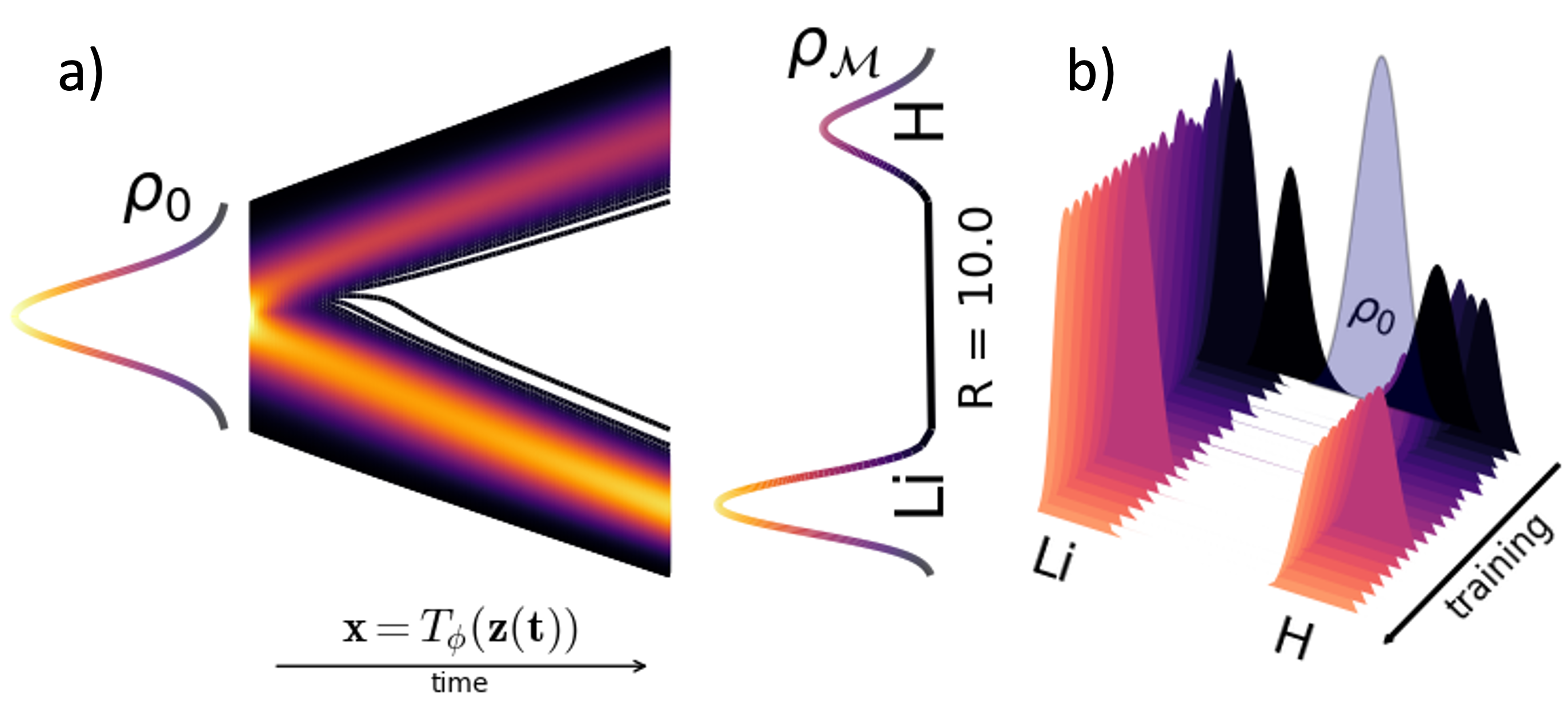
Figure 1: (a) The learned flow, Eq. 5, that minimizes the total energy for the LiH 1-D system for $R=10$ a.u. (b) The change of $\operatorname{\rho_{{\cal M}}}$ at different iterations of the optimization. $\operatorname{\rho_{0}}$ is a zero-centered Gaussian distribution. See the text for more details of the simulations.

Results: To illustrate the use of CNF as $\operatorname{\rho_{{\cal M}}}$ ansatz, we first considered a one-dimensional (1-D) model for diatomic molecules based on Ref. ⁶⁵. For this toy system, we considered the XC functional from Ref. ⁶⁶, and $T_{\text{W}}$ was computed using the score function through Eq. 5, $T_{\text{W}}[\operatorname{\rho_{{\cal M}}}]=\frac{\operatorname{\lambda_{0}}}{8}\int\left(\nabla\log\operatorname{\rho_{{\cal M}}}(x)\right)^{2}\operatorname{\rho_{{\cal M}}}(x)\mathrm{d}x$. The Hartree ($V_{\text{H}}$), and the external potentials ($V_{\text{e-N}}$) both are defined by their soft version, ⁶⁵

$$V_{\text{H}}[\operatorname{\rho_{{\cal M}}}] = \int\int\tfrac{\operatorname{\rho_{{\cal M}}}(x)\operatorname{\rho_{{\cal M}}}(x^{\prime})}{\sqrt{1+|x-x^{\prime}|^{2}}}\mathrm{d}x\mathrm{d}x^{\prime},$$ (8)

$$V_{\text{e-N}}[\operatorname{\rho_{{\cal M}}}] = -\int\biggl{(}\tfrac{Z_{\alpha}}{\sqrt{1+|x-R/2|^{2}}}+\tfrac{Z_{\beta}}{\sqrt{1+|x+R/2|^{2}}}\biggr{)}\operatorname{\rho_{{\cal M}}}(x)\mathrm{d}x.$$

We chose LiH as the 1-D diatomic molecule given the asymmetry due to the mass difference between its atoms; $Z_{\alpha}=3$, $Z_{\beta}=1$. We first considered the inter-atomic distance ($R$) equal to $10$ Bohr. For the estimation of the total energy, we used 512 samples from the base distribution $\operatorname{\rho_{0}}$, a zero-centered Gaussian distribution with $\sigma=1$. Fig. 1 illustrates the learned flow, or mass transport, from $\operatorname{\rho_{0}}$ to $\operatorname{\rho_{{\cal M}}}$ by the CNF (Eq. 5) that minimizes $E[\operatorname{\rho_{{\cal M}}}]$, $\operatorname{N_{e}}=2$. As we can also observe from Figs. 1-2, this CNF ansatz is capable of splitting the density given the large value of $R$ and allocating a higher concentration of electron density closer to the Li nuclei. Our simulations indicate that only $\sim 5,000$ optimization steps were needed for converged results, see Fig. S1 in the SI.

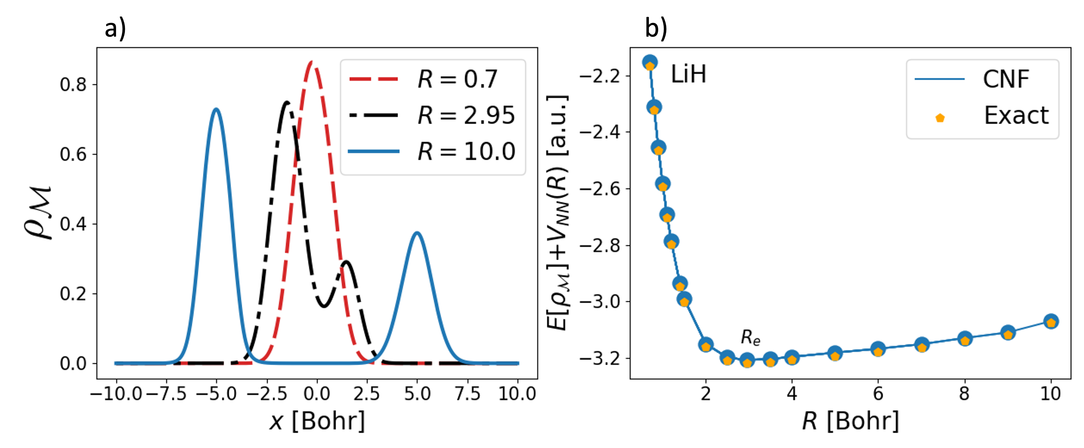
Figure 2: (a) $\operatorname{\rho_{{\cal M}}}$ for LiH for different nuclear distances $R$. For all simulations, $\operatorname{\rho_{0}}$ is a zero-centered Gaussian distribution with $\sigma=1$. (b) The total energy of 1-D LiH as a function of $R$. $V_{\text{NN}}(R)$ is the nuclear repulsion term and $R_{e}=2.95$ a.u. $\pentagofill$-symbols represent the total energy value computed with quadrature integration. See the text for more details of the simulations.

We also investigated the flexibility of the proposed CNF ansatz by considering different ranges of inter-nuclear distances for LiH, Fig. 2, employing the same $\operatorname{\rho_{0}}$ (1-D Gaussian distribution). For all these 1-D simulations, we utilized the same architecture for $\operatorname{g_{\phi}}$, a feed-forward neural network (NN) composed of three hidden layers each with 512 neurons and the $\tanh$ activation function. Other architectures were tested but found to be sub-optimal. Our simulations also reveal that $\operatorname{g_{\phi}}$, when randomly initialized, effectively accelerates the minimization of $E[\operatorname{\rho_{{\cal M}}}]$, particularly at large inter-nuclear distances ($R\gg R_{e}$), where $R_{e}=2.95$ Bohr denotes the equilibrium bond distance. These results demonstrate the flexibility of $\operatorname{g_{\phi}}$ for different scenarios, from strong nuclear interactions ($R<R_{e}$) to bond-breaking regimes ($R\gg R_{e}$), Fig. 2. The potential energy surface curve for the LiH, Fig. 2, further corroborates these findings. In addition, we verified the validity of the proposed MC method by computing the total energy with the learned $\operatorname{\rho_{{\cal M}}}$ employing quadrature integration procedures, and we found no discernible difference in the results, Fig. 2b, and Fig. S1 in the SI.

In normalizing flows, the transformation map $\operatorname{T_{\phi}}$ (Eq. 4) connects the base density, $\operatorname{\rho_{0}}$, with the target density, $\operatorname{\rho_{\phi}}$. While $\operatorname{\rho_{0}}$ is commonly modeled as a multi-variate Gaussian for applications like image generation, in the realm of molecular systems, adopting a promolecular density ($\operatorname{\tilde{\rho}_{0}}$), emerges as a more natural base distribution. This choice not only enhances the base model’s alignment with molecular structures but could also potentially reduce the need for larger $\operatorname{g_{\phi}}$ models. We leverage this uniqueness and define $\operatorname{\tilde{\rho}_{0}}=\sum_{i}c_{i}{\cal N}_{i}(\mathbf{R}_{i},\sigma=1)$, where ${\cal N}_{i}$ is a 1S orbital centered at the nucleus position ($\mathbf{R}_{i}$). The coefficients $c_{i}$ represent the proportional influence of each nucleus on the overall density, $\sum_{i}c_{i}=1$, and $c_{i}=\tfrac{Z_{i}}{\sum_{j}Z_{j}}$ where $Z_{i}$ is the atomic number of the $i^{th}$-nucleus. This alternative base distribution strategy accelerates the optimization process, as $\operatorname{T_{\phi}}$ primarily learns the local changes of $\operatorname{\tilde{\rho}_{0}}$ rather than the global shifts, which would be the case if $\operatorname{\rho_{0}}$ was an arbitrary distribution. To precisely model this density transformation and account for symmetries in the system, $\operatorname{g_{\phi}}$ is a permutation equivariant graph neural network (GNN) ⁶⁷, ⁶⁸,

$$g_{\phi}(\mathbf{z},t)=\sum_{i}^{N_{a}}f_{\phi}(\|\mathbf{z}(t)-\mathbf{R}_{i}\|_{2},\tilde{Z}_{i})(\mathbf{z}(t)-\mathbf{R}_{i}),$$ (10)

where $N_{a}$ is the number of nucleus, $\tilde{Z}_{i}$ is the atomic number of the $i^{th}$-nucleus encoded as a one-hot vector, and $f_{\phi}(\cdot)$ is a two-layer NN with $64$ neurons per layer, and $\tanh$ activation function. This GNN architecture is selected for its capability to process permutations of input atoms invariantly, thereby capturing the essential spatial and chemical properties of the molecule, uninfluenced by the atoms’ order. For $\operatorname{\rho_{{\cal M}}}$ to be permutation invariant with respect to the atoms, the vector field ($\operatorname{g_{\phi}}$) must be permutation equivariant, and $\operatorname{\rho_{0}}$ can be factorized across atoms, meaning permutation invariant ⁴¹, ⁶⁸.

We further investigate the scalability of CNFs through simulations in realistic real-space systems, focusing on the H₂, and H₂O molecular systems. For these molecular systems, the exchange component of $E_{\text{XC}}$ was modeled using a combination of the Local Density Approximation and the B88 exchange functional. For the correlation component $E_{\text{C}}$, we utilized both the PW92  ⁶⁹ and the VWN ⁷⁰, ⁷¹ correlation functionals. Detailed equations are presented in the SI.

For H$2$ with $R=0.7$ Å, we found that $\sim 5,000$ iterations are needed for the total energy to stabilize, as sketched in Fig. 3. We further validate the total energy value using quadrature integration (and MC), -1.2835 (-1.2798) a.u. for the VWN functional, and -1.2837 (-1.2799) a.u. for the PW92 functional. The difference between utilizing $\operatorname{\rho_{0}}$ or $\operatorname{\tilde{\rho}_{0}}$ in this diatomic system is minor, Fig. 3a. We found a $\sim 10^{-3}$ a.u. energy change when $\operatorname{g_{\phi}}$ with an additional layer is considered; see Table S4 for more results. Additionally, Fig. 3b illustrates the change of $\operatorname{\rho_{{\cal M}}}$ through the optimization, notably showcasing an increase in the electron density around the nuclei. As a reference, the total energy for a KS-DFT simulation for the VWN functional with the 6-31G(d,p) (STO-3G) basis set is -1.6133 (-1.5917) a.u. The results for LiH are presented in the SI, Table S4.

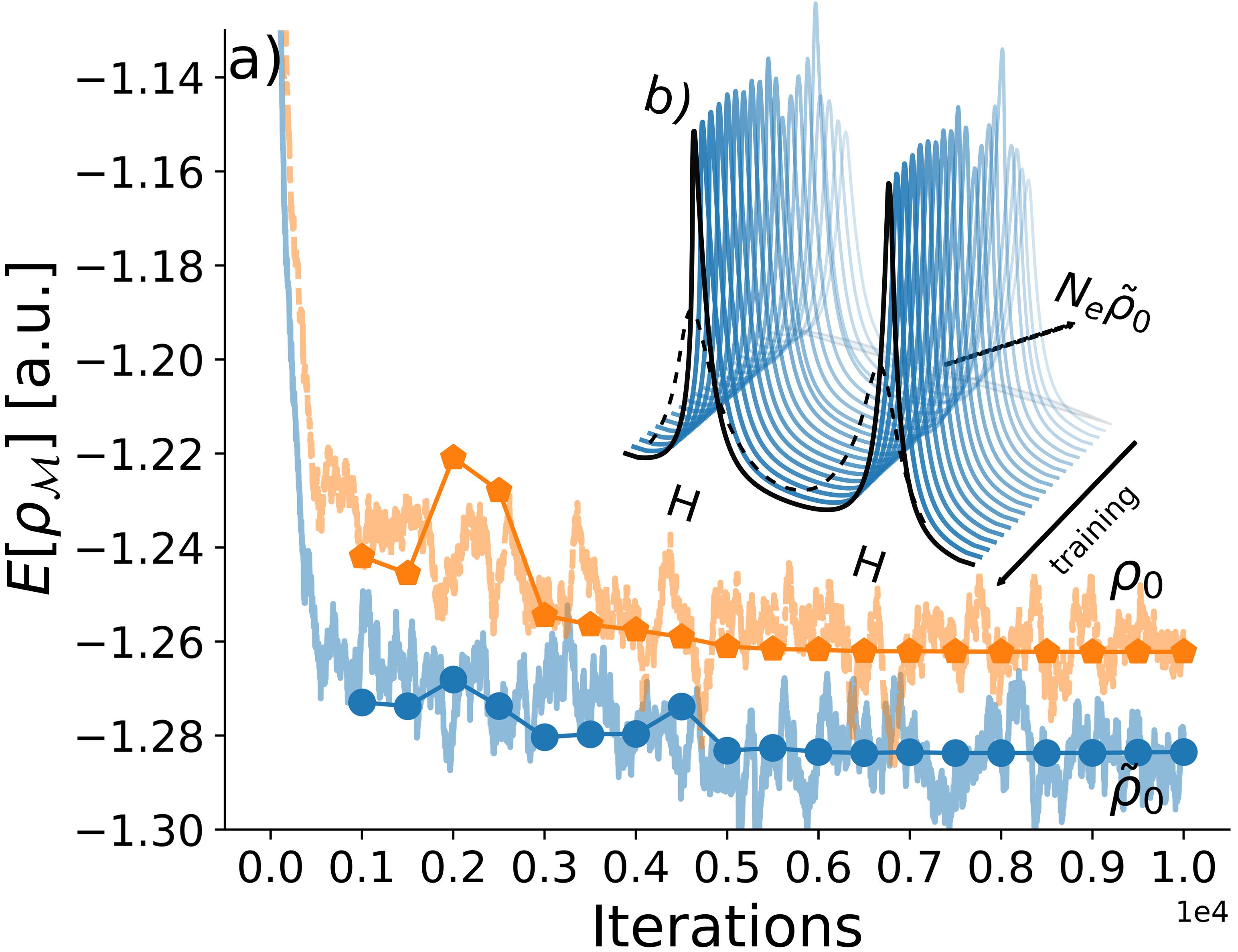
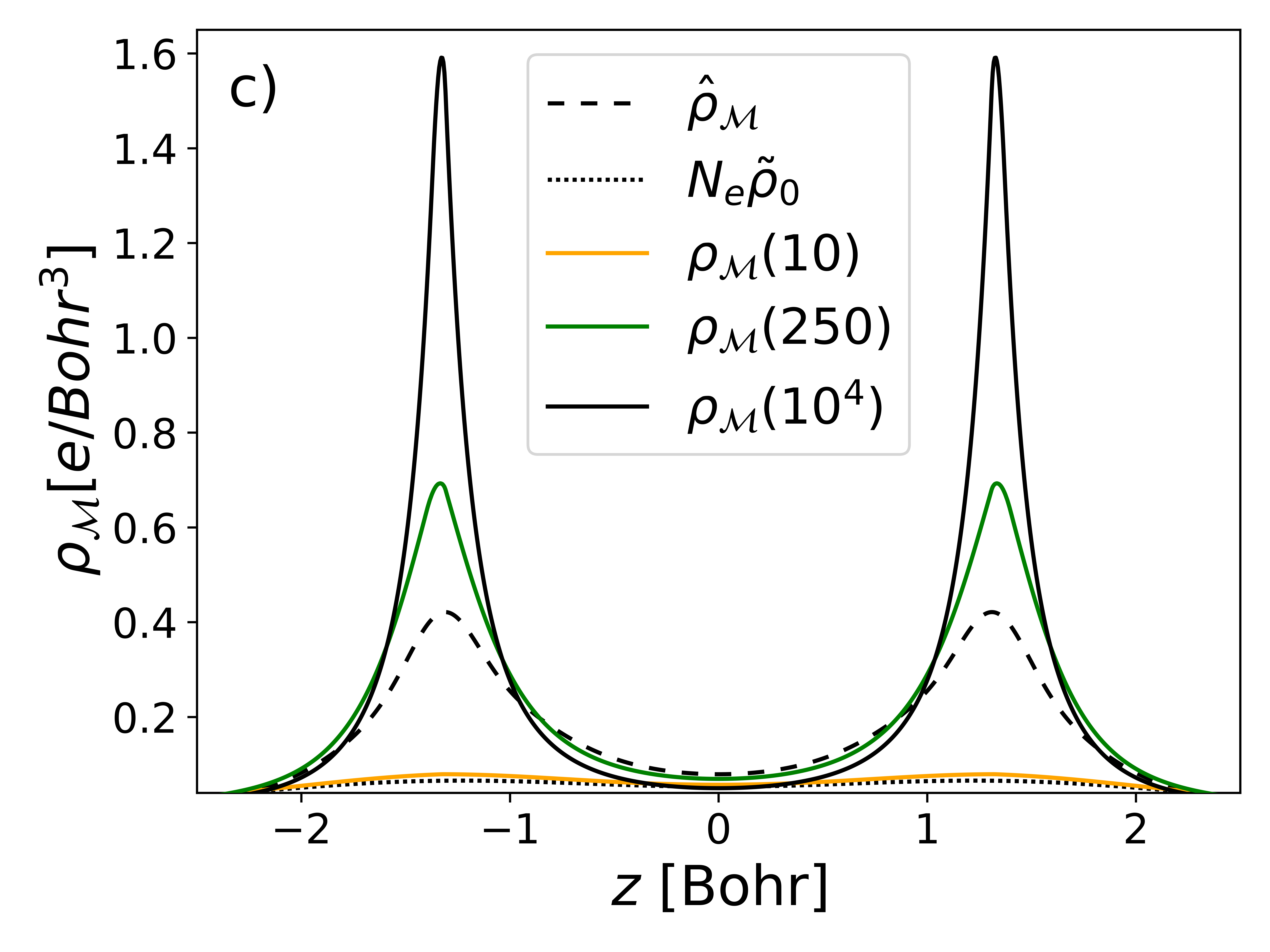
Figure 3: a) The total energy of H₂ molecule through the optimization for a CNF with a single Gaussian distribution ($\operatorname{\rho_{0}}$) and a promolecular density ($\operatorname{\tilde{\rho}_{0}}$). The symbols indicate the total energy computed with quadrature integration and the curves with Monte Carlo. b) and c) The cross-section of the $\operatorname{\rho_{{\cal M}}}$ at various iterations when $\operatorname{\tilde{\rho}_{0}}$ is used. For these simulations, used the VWN functional for the correlation functional. $\operatorname{\hat{\rho}_{{\cal M}}}$ represents the density computed using the KS formalism with a 6-31G(d,p) basis set.

For H₂O, the total energy stabilizes at $\sim 8,000$ iterations when using $\operatorname{\tilde{\rho}_{0}}$. This suggests that the computation of $\nabla_{\phi}E[\operatorname{\rho_{{\cal M}}}]$ in the backward pass, computed with the adjoint method ⁴⁹, is more efficient. This is key for larger systems’ simulations. As opposed to H₂, we found a significant improvement for water when a three-layer GNN was used without a big compromise in the optimization time (see Table S4 in the SI). The total energy, computed with quadrature integration, for the VWN (PW92) functional, is -82.3544 (-82.2378) a.u. The results with $\operatorname{\tilde{\rho}_{0}}$ and the proposed $\operatorname{g_{\phi}}$ architecture (Eq. 10) agree with a KS-DFT simulation using a minimal basis set, which yielded -83.9016 a.u. This energy discrepancy is expected given the level of the KE functional used in the simulations. Additional information on the simulations is presented in the SI.

In normalizing flow-based ansatze, the target density ($\operatorname{\rho_{\phi}}$) is derived by transforming a base distribution using the bijective transformation $\operatorname{T_{\phi}}$. This process effectively “morphs” the base distribution into the target one. As the complexity of the diffeomorphism increases, a larger network or model is needed to capture the $\operatorname{\rho_{0}}\to\operatorname{\rho_{\phi}}$ transformation accurately. For the molecular systems studied in this work, as expected, $\operatorname{T_{\phi}}$ (Eq. 5) learns to primarily increase the electron density closer to the nucleus region, even if a base distribution with no previous knowledge of the location of the nucleus is used. This is illustrated in Fig. 4b, which displays $\log\left|\text{det}\nabla_{\operatorname{\mathbf{z}}}\operatorname{T_{\phi}}(\operatorname{\mathbf{z}})\right|$ mapped over the base distribution for the water molecule. Our findings indicate that in regions proximal to the nucleus, $\operatorname{T_{\phi}}$ effectively enhances electron density, as indicated by the sign of $\log\left|\text{det}\nabla_{\operatorname{\mathbf{z}}}\operatorname{T_{\phi}}(\operatorname{\mathbf{z}})\right|$. In contrast, $\operatorname{T_{\phi}}$ reduces the value of $\operatorname{\rho_{0}}$ in more distant areas, guaranteeing normalization. Fig. 4b further illustrates that $\operatorname{T_{\phi}}$ is unique for the base distribution used.

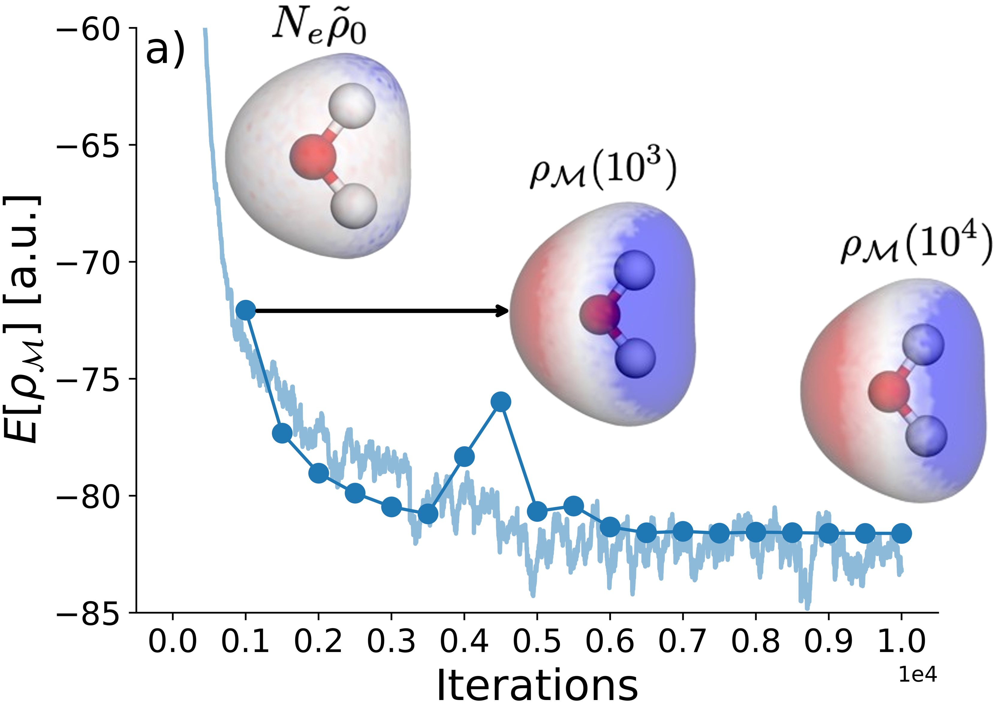
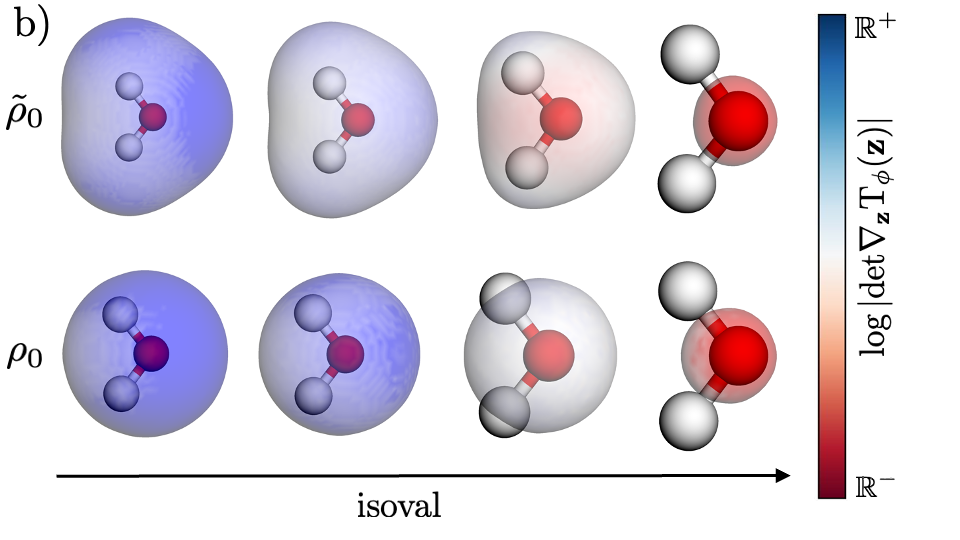
Figure 4: a) The total energy of H₂O molecule through the optimization for a CNF with a promolecular density ($\operatorname{\tilde{\rho}_{0}}$) as the base distributions. The symbols indicate the total energy computed with quadrature integration and the curves with Monte Carlo. For $\operatorname{\rho_{{\cal M}}}$, the color-coded map indicates the value of the molecular electrostatic potential. b) The learned change of density ($\log\left|\text{det}\nabla_{\operatorname{\mathbf{z}}}\operatorname{T_{\phi}}(\operatorname{\mathbf{z}})\right|)$ by the CNF ansatz (Eq. 4) at different values of the base distribution; $\operatorname{\rho_{0}}$ is a single Gaussian distribution. For these simulations, we used the VWN functional.

Summary: In this study, we introduce an innovative framework that utilizes generative models, particularly continuous normalizing flows, to parameterize electron densities in real space within molecular systems. This approach marks a significant shift away from traditional Lagrangian-based formulation within the OF-DFT framework. It distinguishes itself by ensuring direct normalization through ansatz’s architecture and merges the strengths of variational inference with the latest in machine learning optimization and automatic differentiation. Our methodology was tested across various chemical systems and combined with promolecular densities. This initialization step introduces prior physical knowledge into the ansatz, a notable departure from traditional methods.

Furthermore, the integration of generative models into OF-DFT, along with the use of equivariant GNN, complemented by recent advancements in kinetic energy functional development ⁷², ⁷³, ⁷⁴, ⁷⁵, ⁷⁶, ⁷⁷, ⁷⁸, ²¹, ⁷⁹, holds a promising new avenue for the simulation of molecular systems. This novel direction circumvents the limitations associated with grid-based ansatze, paving the way for alternative modeling of chemical systems within the OF-DFT framework.

The authors thank J. Davidsson, R. Armiento, and C. Benavides-Riveros for fruitful discussions. This research was enabled in part by support provided by the Digital Research Alliance of Canada.

References

- Kohn and Sham 1965 Kohn, W.; Sham, L. J. Self-consistent equations including exchange and correlation effects. Physical review 1965, 140, A1133
- Becke 2014 Becke, A. D. Perspective: Fifty years of density-functional theory in chemical physics. The Journal of Chemical Physics 2014, 140, 18A301
- Yu et al. 2016 Yu, H. S.; Li, S. L.; Truhlar, D. G. Perspective: Kohn-Sham density functional theory descending a staircase. The Journal of Chemical Physics 2016, 145, 130901
- Mardirossian and Head-Gordon 2017 Mardirossian, N.; Head-Gordon, M. Thirty years of density functional theory in computational chemistry: an overview and extensive assessment of 200 density functionals. Molecular physics 2017, 115, 2315–2372
- Mardirossian and Head-Gordon 2017 Mardirossian, N.; Head-Gordon, M. Thirty years of density functional theory in computational chemistry: an overview and extensive assessment of 200 density functionals. Molecular Physics 2017, 115, 2315–2372
- Teale et al. 2022 Teale, A. M. et al. DFT exchange: sharing perspectives on the workhorse of quantum chemistry and materials science. Phys. Chem. Chem. Phys. 2022, 24, 28700–28781
- Perdew et al. 1996 Perdew, J. P.; Burke, K.; Ernzerhof, M. Generalized gradient approximation made simple. Physical review letters 1996, 77, 3865
- Stephens et al. 1994 Stephens, P. J.; Devlin, F. J.; Chabalowski, C. F.; Frisch, M. J. Ab initio calculation of vibrational absorption and circular dichroism spectra using density functional force fields. The Journal of physical chemistry 1994, 98, 11623–11627
- Beck 1993 Beck, A. D. Density-functional thermochemistry. III. The role of exact exchange. J. Chem. Phys 1993, 98, 5648–6
- Heyd et al. 2003 Heyd, J.; Scuseria, G. E.; Ernzerhof, M. Hybrid functionals based on a screened Coulomb potential. The Journal of chemical physics 2003, 118, 8207–8215
- Borlido et al. 2020 Borlido, P.; Schmidt, J.; Huran, A. W.; Tran, F.; Marques, M. A.; Botti, S. Exchange-correlation functionals for band gaps of solids: benchmark, reparametrization and machine learning. npj Computational Materials 2020, 6, 1–17
- Vargas-Hernández 2020 Vargas-Hernández, R. A. Bayesian Optimization for Calibrating and Selecting Hybrid-Density Functional Models. The Journal of Physical Chemistry A 2020, 124, 4053–4061, PMID: 32338905
- Li et al. 2021 Li, L.; Hoyer, S.; Pederson, R.; Sun, R.; Cubuk, E. D.; Riley, P.; Burke, K. Kohn-Sham Equations as Regularizer: Building Prior Knowledge into Machine-Learned Physics. Phys. Rev. Lett. 2021, 126, 036401
- Cuierrier et al. 2021 Cuierrier, E.; Roy, P.-O.; Ernzerhof, M. Constructing and representing exchange–correlation holes through artificial neural networks. The Journal of Chemical Physics 2021, 155, 174121
- Wu et al. 2023 Wu, J.; Pun, S.-M.; Zheng, X.; Chen, G. Construct exchange-correlation functional via machine learning. The Journal of Chemical Physics 2023, 159, 090901
- Kirkpatrick et al. 2021 Kirkpatrick, J.; McMorrow, B.; Turban, D. H.; Gaunt, A. L.; Spencer, J. S.; Matthews, A. G.; Obika, A.; Thiry, L.; Fortunato, M.; Pfau, D., et al. Pushing the frontiers of density functionals by solving the fractional electron problem. Science 2021, 374, 1385–1389
- Ma et al. 2022 Ma, H.; Narayanaswamy, A.; Riley, P.; Li, L. Evolving symbolic density functionals. Science Advances 2022, 8, eabq0279
- Hohenberg and Kohn 1964 Hohenberg, P.; Kohn, W. Inhomogeneous electron gas. Physical review 1964, 136, B864
- Parr and Yang 1980 Parr, R. G.; Yang, W. Density Functional Theory of Atoms and Molecules. Horizons of Quantum Chemistry. Dordrecht, 1980; pp 5–15
- Zhang et al. 2024 Zhang, H.; Liu, S.; You, J.; Liu, C.; Zheng, S.; Lu, Z.; Wang, T.; Zheng, N.; Shao, B. Overcoming the barrier of orbital-free density functional theory for molecular systems using deep learning. Nature Computational Science 2024, 1–14
- Mazo-Sevillano and Hermann 2023 Mazo-Sevillano, P. d.; Hermann, J. Variational principle to regularize machine-learned density functionals: The non-interacting kinetic-energy functional. The Journal of Chemical Physics 2023, 159
- Hodges 1973 Hodges, C. Quantum corrections to the Thomas–Fermi approximation—the Kirzhnits method. Canadian Journal of Physics 1973, 51, 1428–1437
- Brack et al. 1976 Brack, M.; Jennings, B.; Chu, Y. On the extended Thomas-Fermi approximation to the kinetic energy density. Physics Letters B 1976, 65, 1–4
- Wang and Teter 1992 Wang, L.-W.; Teter, M. P. Kinetic-energy functional of the electron density. Physical Review B 1992, 45, 13196
- Perrot 1994 Perrot, F. Hydrogen-hydrogen interaction in an electron gas. Journal of Physics: Condensed Matter 1994, 6, 431
- Wang et al. 1998 Wang, Y. A.; Govind, N.; Carter, E. A. Orbital-free kinetic-energy functionals for the nearly free electron gas. Physical Review B 1998, 58, 13465
- Huang and Carter 2010 Huang, C.; Carter, E. A. Nonlocal orbital-free kinetic energy density functional for semiconductors. Physical Review B 2010, 81, 045206
- Smargiassi and Madden 1994 Smargiassi, E.; Madden, P. A. Orbital-free kinetic-energy functionals for first-principles molecular dynamics. Physical Review B 1994, 49, 5220
- Foley and Madden 1996 Foley, M.; Madden, P. A. Further orbital-free kinetic-energy functionals for ab initio molecular dynamics. Physical Review B 1996, 53, 10589
- Mi et al. 2018 Mi, W.; Genova, A.; Pavanello, M. Nonlocal kinetic energy functionals by functional integration. The Journal of Chemical Physics 2018, 148
- Pedregosa et al. 2011 Pedregosa, F. et al. Scikit-learn: Machine Learning in Python. Journal of Machine Learning Research 2011, 12, 2825–2830
- O’shea and Nash 2015 O’shea, K.; Nash, R. An introduction to convolutional neural networks. arXiv preprint arXiv:1511.08458 2015,
- He et al. 2016 He, K.; Zhang, X.; Ren, S.; Sun, J. Deep residual learning for image recognition. Proceedings of the IEEE conference on computer vision and pattern recognition. 2016; pp 770–778
- David M. Blei and McAuliffe 2017 David M. Blei, A. K.; McAuliffe, J. D. Variational Inference: A Review for Statisticians. Journal of the American Statistical Association 2017, 112, 859–877
- Lecun et al. 2006 Lecun, Y.; Chopra, S.; Hadsell, R.; Ranzato, M.; Huang, F. In Predicting structured data; Bakir, G., Hofman, T., Scholkopt, B., Smola, A., Taskar, B., Eds.; MIT Press, 2006
- Bu and Wang 2023 Bu, L.-Z.; Wang, W. Efficient single-grid and multi-grid solvers for real-space orbital-free density functional theory. Computer Physics Communications 2023, 290, 108778
- Natarajan et al. 2011 Natarajan, B.; Casida, M. E.; Genovese, L.; Deutsch, T. Wavelets for density-functional theory and post-density-functional-theory calculations. arXiv preprint arXiv:1110.4853 2011,
- Chan et al. 2001 Chan, G. K.-L.; Cohen, A. J.; Handy, N. C. Thomas-Fermi-Dirac-von Weizsäcker models in finite systems. The Journal of Chemical Physics 2001, 114, 631–638
- Parr and Bartolotti 1983 Parr, R. G.; Bartolotti, L. J. Some remarks on the density functional theory of few-electron systems. The Journal of Physical Chemistry 1983, 87, 2810–2815
- Kobyzev et al. 2020 Kobyzev, I.; Prince, S. J.; Brubaker, M. A. Normalizing flows: An introduction and review of current methods. IEEE transactions on pattern analysis and machine intelligence 2020, 43, 3964–3979
- Papamakarios et al. 2021 Papamakarios, G.; Nalisnick, E.; Rezende, D. J.; Mohamed, S.; Lakshminarayanan, B. Normalizing flows for probabilistic modeling and inference. The Journal of Machine Learning Research 2021, 22, 2617–2680
- Rezende and Mohamed 2015 Rezende, D.; Mohamed, S. Variational inference with normalizing flows. International conference on machine learning. 2015; pp 1530–1538
- Cranmer et al. 2019 Cranmer, K.; Golkar, S.; Pappadopulo, D. Inferring the quantum density matrix with machine learning. arXiv preprint arXiv:1904.05903 2019,
- Saleh et al. 2023 Saleh, Y.; Álvaro Fernández Corral,; Iske, A.; Küpper, J.; Yachmenev, A. Computing excited states of molecules using normalizing flows. 2023
- Thiede et al. 2022 Thiede, L.; Sun, C.; Aspuru-Guzik, A. Waveflow: Enforcing boundary conditions in smooth normalizing flows with application to fermionic wave functions. arXiv preprint arXiv:2211.14839 2022,
- David and Danilo 2020 David, P.; Danilo, R. Integrable Nonparametric Flows. 2020
- James et al. 2023 James, S.; Brian, C.; Shravan, V. Numerical and geometrical aspects of flow-based variational quantum Monte Carlo. Machine Learning: Science and Technology 2023, 4, 021001
- Li et al. 2023 Li, T.; Lin, M.; Hu, Z.; Zheng, K.; Vignale, G.; Kawaguchi, K.; Neto, A.; Novoselov, K. S.; Yan, S. D4FT: A Deep Learning Approach to Kohn-Sham Density Functional Theory. arXiv preprint arXiv:2303.00399 2023,
- Chen et al. 2018 Chen, R. T.; Rubanova, Y.; Bettencourt, J.; Duvenaud, D. K. Neural ordinary differential equations. Advances in neural information processing systems 2018, 31
- Shuangshuang et al. 2023 Shuangshuang, C.; Sihao, D.; Yiannis, K.; Mårten, B. Learning Continuous Normalizing Flows For Faster Convergence To Target Distribution via Ascent Regularizations. The Eleventh International Conference on Learning Representations. 2023
- Mohamed et al. 2020 Mohamed, S.; Rosca, M.; Figurnov, M.; Mnih, A. Monte carlo gradient estimation in machine learning. Journal of Machine Learning Research 2020, 21, 1–62
- M. Casares et al. 2024 M. Casares, P. A.; Baker, J. S.; Medvidović, M.; Reis, R. d.; Arrazola, J. M. GradDFT. A software library for machine learning enhanced density functional theory. 2024; https://doi.org/10.1063/5.0181037
- Arrazola et al. 2023 Arrazola, J. M. et al. Differentiable quantum computational chemistry with PennyLane. 2023
- Kasim and Vinko 2021 Kasim, M. F.; Vinko, S. M. Learning the Exchange-Correlation Functional from Nature with Fully Differentiable Density Functional Theory. Phys. Rev. Lett. 2021, 127, 126403
- Tamayo-Mendoza et al. 2018 Tamayo-Mendoza, T.; Kreisbeck, C.; Lindh, R.; Aspuru-Guzik, A. Automatic Differentiation in Quantum Chemistry with Applications to Fully Variational Hartree–Fock. ACS Central Science 2018, 4, 559–566, PMID: 29806002
- Vargas-Hernández et al. 2021 Vargas-Hernández, R. A.; Chen, R. T. Q.; Jung, K. A.; Brumer, P. Fully differentiable optimization protocols for non-equilibrium steady states. New Journal of Physics 2021, 23, 123006
- Vargas–Hernández et al. 2023 Vargas–Hernández, R. A.; Jorner, K.; Pollice, R.; Aspuru–Guzik, A. Inverse molecular design and parameter optimization with Hückel theory using automatic differentiation. The Journal of Chemical Physics 2023, 158, 104801
- Dawid et al. 2023 Dawid, A. et al. Modern applications of machine learning in quantum sciences. 2023
- Zhang and Chan 2022 Zhang, X.; Chan, G. K.-L. Differentiable quantum chemistry with PySCF for molecules and materials at the mean-field level and beyond. The Journal of Chemical Physics 2022, 157, 204801
- Schmidt et al. 2019 Schmidt, J.; Benavides-Riveros, C. L.; Marques, M. A. Machine learning the physical nonlocal exchange–correlation functional of density-functional theory. The journal of physical chemistry letters 2019, 10, 6425–6431
- Tan et al. 2023 Tan, C. W.; Pickard, C. J.; Witt, W. C. Automatic differentiation for orbital-free density functional theory. The Journal of Chemical Physics 2023, 158
- Costa et al. 2022 Costa, E.; Scriva, G.; Fazio, R.; Pilati, S. Deep-learning density functionals for gradient descent optimization. Phys. Rev. E 2022, 106, 045309
- Tieleman et al. 2012 Tieleman, T.; Hinton, G., et al. Lecture 6.5-RMSProp: Divide the gradient by a running average of its recent magnitude. COURSERA: Neural networks for machine learning 2012, 4, 26–31
- Bradbury et al. 2018 Bradbury, J.; Frostig, R.; P.Hawkins,; Johnson, M.; Leary, C.; Maclaurin, D.; Necula, G.; Paszke, A.; VanderPlas, J.; Wanderman-Milne, S.; Zhang, Q. JAX: composable transformations of Python+NumPy programs. 2018; http://github.com/google/jax
- Snyder et al. 2013 Snyder, J. C.; Rupp, M.; Hansen, K.; Blooston, L.; Müller, K.; Burke, K. Orbital-free bond breaking via machine learning. The Journal of chemical physics 2013, 139
- Shulenburger et al. 2009 Shulenburger, L.; Casula, M.; Senatore, G.; Martin, R. M. Spin resolved energy parametrization of a quasi-one-dimensional electron gas. Journal of Physics A: Mathematical and Theoretical 2009, 42, 214021
- Köhler et al. 2020 Köhler, J.; Klein, L.; Noe, F. Equivariant Flows: Exact Likelihood Generative Learning for Symmetric Densities. Proceedings of the 37th International Conference on Machine Learning. 2020; pp 5361–5370
- Zwartsenberg et al. 2023 Zwartsenberg, B.; Scibior, A.; Niedoba, M.; Lioutas, V.; Sefas, J.; Liu, Y.; Dabiri, S.; Lavington, J. W.; Campbell, T.; Wood, F. Conditional Permutation Invariant Flows. Transactions on Machine Learning Research 2023,
- Perdew and Wang 1992 Perdew, J. P.; Wang, Y. Accurate and simple analytic representation of the electron-gas correlation energy. Physical review B 1992, 45, 13244
- Vosko et al. 1980 Vosko, S. H.; Wilk, L.; Nusair, M. Accurate spin-dependent electron liquid correlation energies for local spin density calculations: a critical analysis. Canadian Journal of physics 1980, 58, 1200–1211
- Shulenburger et al. 2009 Shulenburger, L.; Casula, M.; Senatore, G.; Martin, R. M. Spin resolved energy parametrization of a quasi-one-dimensional electron gas. Journal of Physics A: Mathematical and Theoretical 2009, 42, 214021
- Zhang et al. 2024 Zhang, H.; Liu, S.; You, J.; Liu, C.; Zheng, S.; Lu, Z.; Wang, T.; Zheng, N.; Shao, B. Overcoming the barrier of orbital-free density functional theory for molecular systems using deep learning. Nature Computational Science 2024,
- Sun and Chen 2023 Sun, L.; Chen, M. Machine-Learning-Based Non-Local Kinetic Energy Density Functional for Simple Metals and Alloys. arXiv preprint arXiv:2310.15591 2023,
- Seino et al. 2018 Seino, J.; Kageyama, R.; Fujinami, M.; Ikabata, Y.; Nakai, H. Semi-local machine-learned kinetic energy density functional with third-order gradients of electron density. The Journal of chemical physics 2018, 148
- Fujinami et al. 2020 Fujinami, M.; Kageyama, R.; Seino, J.; Ikabata, Y.; Nakai, H. Orbital-free density functional theory calculation applying semi-local machine-learned kinetic energy density functional and kinetic potential. Chemical Physics Letters 2020, 748, 137358
- Manzhos and Golub 2020 Manzhos, S.; Golub, P. Data-driven kinetic energy density fitting for orbital-free DFT: Linear vs Gaussian process regression. The Journal of Chemical Physics 2020, 153
- Seino et al. 2019 Seino, J.; Kageyama, R.; Fujinami, M.; Ikabata, Y.; Nakai, H. Semi-local machine-learned kinetic energy density functional demonstrating smooth potential energy curves. Chemical Physics Letters 2019, 734, 136732
- Meyer et al. 2020 Meyer, R.; Weichselbaum, M.; Hauser, A. W. Machine learning approaches toward orbital-free density functional theory: Simultaneous training on the kinetic energy density functional and its functional derivative. Journal of chemical theory and computation 2020, 16, 5685–5694
- Benavides-Riveros 2024 Benavides-Riveros, C. L. Orbital-free quasidensity functional theory. Physical Review Research 2024, 6, 013060