Strategic Informed Trading and the Value of Private Information

Michail Anthropelos Department of Banking and Financial Management
University of Piraeus
Piraeus, Greece
anthropel@unipi.gr
 and  Scott Robertson Questrom School of Business
Boston University
Boston, MA 02215
scottrob@bu.edu
Abstract.

We consider a market of risky financial assets where the participants are an informed trader, a mass of uniformed traders and noisy liquidity providers. We prove the existence of a market-clearing equilibrium when the insider internalizes her power to impact prices. In the price-impact equilibrium the insider strategically reveals a noisier (compared to when the insider takes prices as given) signal, and prices are less reactive to the publicly available information. In contrast to the related literature, we show that in the price-impact equilibrium, the insider’s ex-ante welfare monotonically increases in the signal precision. This clarifies when a trader with market power is motivated to both obtain and refine her private information. Furthermore, even though the uniformed traders act as price-takers, the effect of price impact is ex-ante welfare improving for them. By contrast, internalization of price impact may reduce insider ex-ante welfare. This happens provided the insider is sufficiently risk averse and the uninformed traders are sufficiently risk tolerant.

Introduction

It is well-documented that large financial institutions possess the power to affect markets (see, for example, Koijen and Yogo (2019) and the related discussion in Rostek and Yoon (2023)). Compared to other traders, orders coming from large investors impact both transaction prices and volumes, and large investors are aware of this impact (see Rostek and Weretka (2015a)). Large financial institutions are additionally known to invest considerable capital to acquire information regarding the payoffs of the assets they trade (c.f. Kacperczyk and Pagnotta (2019)). In sum, it is natural to assume that large investors are both (1) aware of their impact on prices and (2) in possession of private information and hence are “insiders” compared to the other traders.

That large investors are informed traders is not a secret. Indeed, the rest of the market knows large investors have private information (see Subrahmanyam (1991)), and as such, the uninformed traders’ account for the insider’s superior information, and expect that in equilibrium there is a partial transmission of private information. In both the price-taking (see Grossman and Stiglitz (1980)) and price-impact (see Kyle (1985)) cases, it is shown that in the presence of noise traders, the insider’s private signal is partially revealed to the uniformed traders through equilibrium prices, a mechanism that creates a market (or public) signal. Therefore, it is reasonable to assume that not only will the insider, who is also aware of her market power, strategically choose the signal she reveals to the market, but also that the uniformed traders recognise, and account for, this fact.

Using the above as motivation, our goal is to study how the insider’s awareness of price impact affects equilibrium prices, information transmission and agent welfare. We work in the classic single period normal-CARA setting, seeking a linear price-impact equilibrium where a risk averse insider (endowed with private information) trades a bundle of risky assets with a mass of uniformed risk-averse traders, as well as liquidity providers (noise traders). We use this model to predict how the insider (partially) reveals her signal; how the uniformed agents correspondingly adjust their demands; and if the informational content within equilibrium prices is reduced compared to when all agents act as price takers.

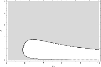
We are also interested in agent welfare. Here, we wish to know if internalization of price impact is welfare improving for the insider and/or the uninformed agent, and especially if the insider’s welfare increases with her signal precision. The latter question arises because in the price-taking equilibrium of Grossman and Stiglitz (1980), insider welfare does not always increase with the signal precision. More precisely, if the insider receives the signal $G=X+Z_{I}$ where $X$ is the asset payoff and $Z_{I}$ is a noise term with precision $p_{I}$, then the map “$p_{I}\to\textrm{Insider Welfare}$” is not monotonically increasing. This is shown in comparison to the price-impact case in Figure 1 below, but qualitatively the map takes the two forms shown in the figure.

[Uncaptioned image]

This is problematic, because either it is never advantageous to obtain the signal (the dot-dashed line) or it is beneficial to obtain the signal, but not to refine it beyond a certain precision level (solid line). As presumably there is a cost (in terms of money and/or effort) to produce the signal, the former case suggests price taking equilibria with private signals are somewhat artificial, and the latter case requires the insider to estimate model parameters (which are very hard to estimate especially for other agents) to know if she should try and improve her signal.

Given this, we would like to know in what environment the insider can be assured that a better quality signal is always better for her, and evidently this is not the case when all agents take prices as given. Furthermore, lack of monotonicity was also shown in the recent Nezafat and Schroder (2023) where all agents account for price impact. However, in our model, by differentiating the insider on two fronts: private information and internalization of market power, we establish monotonicity with respect to the signal precision (Proposition 3.2), and avoid the paradoxical situations where the insider is not motivated to refine her signal, even if doing so does not incur additional costs.

Methodology and Main Contributions

We adjust the single period CARA-normal setting of Grossman and Stiglitz (1980)111Grossman and Stiglitz (1980) assumes all traders are price takers, an assumption ubiquitous in the literature on equilibrium under heterogeneous information. Indeed, it was assumed in the seminal papers of Grossman (1976), Grossman and Stiglitz (1980) and Hellwig (1980), and with the exception of the literature strand started by Kyle (1985); Back (1992), Rochet and Vila (1994) and Subrahmanyam (1991), price taking has remained the dominant assumption. by allowing the insider to internalize her price impact, while maintaining the presence of price-taking uniformed traders and liquidity providers222Assuming the uninformed traders are price takers is realistic, as they represent a mass of small risk-averse traders who rationally optimize their positions, but do not have the power to move prices.. Following the related literature (e.g. Kyle (1985); Rochet and Vila (1994)), we study a linear impact equilibrium where the insider perceives the market price to be an affine function of the sum of her and the noise traders’ demand333Linear price-impact is common in the literature (see among others Kyle (1989), Vayanos (1999), Vives (2011)), and the affine structure of price impact is also seen (though not perceived a-priori by the insider) in the price taking, or competitive, equilibrium (see (26) below)., with the affine coefficients endogenously determined through market clearing.

Our first main result (Theorem 1.6) establishes existence of an affine price impact equilibrium. The affine coefficients (which are not the same as in the price-taking case), are governed by the unique positive root of a certain cubic equation, given in (18)444This stands in contrast to Subrahmanyam (1991) where equilibria are governed by solutions to a quintic equation. The difference arises because, consistent with Grossman and Stiglitz (1980) (see also Rochet and Vila (1994)) we assume the insider, by viewing both her demand and the resultant price, is able to deduce the noise trader’s demand.. For the sake of comparison, we summarize the price-taking results of Grossman and Stiglitz (1980) in Proposition 1.7, and for both the price taking and price impact cases we establish equilibria absent private information by showing it coincides with the zero precision limit: see Proposition 1.11.

Having established existence of equilibria we perform a comparison analysis. While analysis of information transmission and price reactivity yields expected conclusions, the study of indirect utilities (or welfare) results in surprising and novel outcomes that stand in sharp contrast to the literature. Relating to information transmission, we show (similarly to Kacperczyk et al. (2023)) that the insider’s price impact makes the market signal fuzzier than in the competitive setting (see Proposition 2.1). This is reasonable, as the insider has a motive to hide her signal when submitting her demand, and hence her trading lowers the precision of the signal revealed by the prices. Conversely, the uniformed traders recognize the insider reveals a muddied signal, and respond with a less elastic demand function, which in turn makes the equilibrium price less reactive to the public information (consistent with the adverse-selection concerns of Kyle (1989) and Lou and Rahi (2023)). These results are robust across model parameter values (in particular the uninformed traders and insider need not have the same risk aversion) and we conclude that by assuming the insider is a price taker, one is implicitly assuming the market gets a more precise signal, and prices are more reactive to public information, than if the insider had internalized price impact.

We then turn our attention to traders’ indirect utility, which (with a slight abuse of terminology) we refer to as “welfare”. Our main result is that when the insider internalizes price impact (and the uninformed agents do not), insider ex-ante welfare is monotonically increasing in the private signal precision. As discussed above, this result does not hold when either (i) all agents are price takers (e.g. Grossman and Stiglitz (1980)) or (ii) all agents internalize price impact (e.g. Nezafat and Schroder (2023)). Thus, in the reasonable setting of a strategic insider, price-taking uniformed traders and noisy liquidity providers, the meaningful statement “better information increases welfare” always holds, and there is always an incentive to refine the signal. Qualitatively, this result holds because the insider’s strategic trading increases the value of her private signal, and hence refining her signal is attractive.

Our second welfare result stems from a desire to isolate the effects of price impact internalization and private information on insider welfare. In other words, we ask: can one attribute any gain (or loss) in agent welfare to just price impact internalization or just asymmetric information? To answer this, we must turn on and off both the internalization of impact and private information (hence the need for the four equilibria established in Section 1). Our comparison analysis yields several interesting outcomes. First, we show that absent a private signal, internalizing price impact always improves insider welfare. While this result may be expected at the ex-ante level, remarkably it holds for any realization of the noise trader demand. Hence, under symmetric information, the equilibrium at which the insider acts strategically (solely due to her market power) yields a higher utility gain. We conclude that price impact internalization alone increases insider welfare.

The situation changes when we layer in the private signal. While typically (i.e. across the bulk of the parameter space) internalization of price impact yields higher insider welfare, insider welfare does not always increase. Indeed, when the insider is sufficiently risk averse, the uninformed traders are sufficiently risk tolerant and the variance of noise demand is sufficiently low555Note that the variance of noise traders demand can be seen as a proxy for the size of their trading. This approach has been used by Kovalenkov and Vives (2014a) and more recently by Nezafat and Schroder (2023)., internalization of price impact actually reduces the insider’s welfare (the exact condition is given in equation (36) of Proposition 3.6).

This holds because having private information reduces the asset’s risk for the insider, which in turn increases her expected demand (in line with the empirical evidence of Kacperczyk and Pagnotta (2019)). On the other hand, internalization of price impact makes her “hide” her private signal, and this is expected to reduce her demand. This means that price impact and private signal have opposite expected effects on the insider’s demand. While the equilibrium price decreases due to price impact, the insider’s demand is lower under the presence of signal when she is also sufficiently risk averse. If, in addition, the uniformed traders are highly risk tolerant, their demand increases and the insider’s trade at market-clearing equilibrium is reduced even further. In other words, under a large deviation of the traders’ risk aversions, the effect of price impact is dominated by the that of heterogeneous information, the insider’s demand is reduced and her utility gain is lower. However, when the traders have the same risk aversion, the effect of price-impact internalization is always beneficial for the insider. We conclude that both asymmetric information and deviation of agent risk aversions may reduce insider welfare in the price-impact equilibrium. Further details are given in Section 4.

The above results underscore an important (and clarifying) fact. As long as the insider internalizes her price impact, equilibrium prices cannot be driven to the corresponding price-taking equilibrium ones. This stems from the uniformed traders’ optimal demand. Although they are price takers, when determining their optimal demand, they do recognize that the insider internalizes her price impact. As mentioned above, price impact reduces public signal’s precision, and hence uniformed traders demand becomes less elastic than in the competitive equilibrium, and this is true for any realization of the public signal and level of prices. The lower sensitivity on the public signal alters the intercept point of their demand function (as it depends on public signal). Hence, in the price-impact equilibrium the insider trades against a different residual demand than in the price-taking equilibrium, which implies that price-taking equilibrium cannot be written as a special case of the price-impact one.

Finally, analysis of the uniformed traders’ welfare also yields quite interesting outcomes. First, traders are at the same side of trade in both the price-impact and price taking equilibria (e.g. in both equilibria, all agents either buy or sell off their initial endowments). As the insider’s price impact decreases the equilibrium prices, the uniformed traders satisfy their optimal demand at a discount, due to the insider’s price impact. This holds regardless the presence of private signal, which means that price impact is ex-ante beneficial for the uniformed traders with and without asymmetric information, as shown in Proposition 3.5. This allows us to conclude that for the bulk of the parameter space, aggregate welfare of both insider and uniformed traders increases due to the internalization of price impact, and this holds with and without the private signal.

Connection with the related literature

Our paper contributes to the on-going literature on price-impact equilibria under asymmetric information, on market participants’ welfare and on the informativeness of equilibrium prices.

In our price-impact equilibrium, the insider does not act as price-taker. Usually, the price-taking assumption is made for tractability, as in its absence one must specify a price impact model, and depending upon the specification, it may be very difficult to establish equilibria. In the aforementioned Kyle (1985); Back (1992); Rochet and Vila (1994), the insider’s demand is combined with exogenous noise traders’ demand before being sent to a risk neutral market maker who prices in a competitive environment. In Subrahmanyam (1991), market makers are allowed to be risk averse while quoting prices to remain at utility indifference (as opposed the uninformed agent of Grossman and Stiglitz (1980) who can be thought of as a market maker who quotes utility-optimal prices), but the insider does not know the noise trader demand before submitting her order (as in Kyle (1985)). Regarding Subrahmanyam (1991), our analysis updates in two directions. First, by assuming the uninformed agent is a utility optimizer, and second, by allowing the insider to the identify the noise trader demand through the public equilibrium price (as in Rochet and Vila (1994)).

In the spirit of the seminal work of Kyle (1989), several models on normal-CARA setting with price-impact and asymmetric information have been developed. For example, Vayanos (2001) and Rostek and Weretka (2015a) study dynamic thin markets with and without market makers respectively, Rostek and Weretka (2015b) emphasizes on the traders’ interdependent preferences and correlated private signals, while Malamud and Rostek (2017) and Anthropelos and Kardaras (2024) consider decentralized exchanges and restricted participation settings respectively. Also, Bergemann et al. (2021) studies a market of divisible goods where agents receive correlated signals and their demand affects the revealed signal at equilibrium, as in our model. In these works, as in Kyle (1989) and Vives (2011), strategic agents submit demand schedule forming a Nash equilibrium. In contrast to our model, they consider all non-noise agents to be strategic, with private information mostly appearing only on investors’ endowments. An extensive recent overview of this literature is provided in Rostek and Yoon (2023).

While it is an undoubted fact that large financial institutions invest to obtain private information, even when trading in markets that are not thin, theoretical studies that justify the positive relation between better information and higher gains from trading are scarce. We highlight that a key factor which always leads to this positive relationship is the insider’s market power in a markets with a mass of small uniformed traders and noisy liquidity providers. Under a competitive market setting, the fact that private information has positive value if an investor acts strategically was pointed out back in Hirshleifer (1971), while similar positive effect of private signal on traders’ welfare is shown in a competitive model with a continuum of traders in Morris and Shin (2002).

Under non-competitive market settings, information acquisition has been relatively recently studied in Vives (2011), Rostek and Weretka (2012) and Vives (2014), where insiders with correlated noisy signals are considered. An extension of these papers to a two-stage model has been recently developed in Nezafat and Schroder (2023). Therein, at the first stage, one type of traders can choose the precision of the private signal that they will get before trading. This situation is comparable to our model when the rest of the non-noise traders are uniformed (no private signal). In contrast to our model however, both the insider and uniformed traders are assumed strategic, which essentially implies that the market is thin despite the presence of noise traders. Strategic uniformed traders, together with specific conditions on noise traders’ demand, lead to an equilibrium at which private information is welfare-deteriorating. We show that the existence of zero-information equilibria is not possible if the uniformed traders are price takers. In this case, the insider’s ex-ante welfare is always increasing with respect to signal’s precision, which means that the private information does have positive value for the insider. In addition, we show that under Pareto-allocated initial endowments, private information has positive value for uniformed traders too (even though they are assumed as price-takers).

On the other hand, Kacperczyk et al. (2023) considers strategic informed and price-takers uniformed traders as we do, where the role of initial endowments is highlighted for different types of informed traders. In Gong et al. (2022) the insider is assumed risk neutral and the role of uniformed traders is played by an ambiguous market maker with a quadratic objective. A linear equilibrium, similar to Kyle (1985), is derived where the price is underreacted to public signal, as in our case.

Strategic agents and asymmetric information have been included in Lou and Rahi (2023), where in a non-competitive market (in line with Kyle (1989) and Rostek and Weretka (2015a)) traders receive different ex-ante random values of a single asset (and potentially different private signals too). In contrast to our model (and to Kyle (1989)) there are no liquidity providers, which essentially implies that price informativeness does not change due to price impact. As in our model, there are conditions that lead to higher ex-ante expected utility for the uniformed traders than the insider. We reach a similar conclusion, but without assuming that uniformed traders act strategically.

Another channel on the valuation of private information that leads to insider’s lower gains from trading due to private information is the information sharing. For example, Goldstein et al. (2023) reach to this result in a novel model (based on Kyle (1989)) where informed traders share their private signals before trading (as in Indjejikian et al. (2014)).

Structure of the paper

The rest of the paper is organized as follows. In Section 1 provide the model and establish existence of the equilibria under consideration. Section 2 develops quantitative analysis and qualitative discussion on information transmission and signal and price sensitivities. Section 3 focuses on welfare comparison at different equilibria and Section 4 is dedicated to equilibria structure regarding prices and risk allocation and concludes with a discussion on model’s predictions. An extension to a general multi asset model is provided in Appendix A and all proofs are given, starting in Appendix B.


1. The Equilibrium

We now present the model and construct the equilibrium. To both isolate the effects of price impact internalization and asymmetric information, and to keep the presentation/notation as simple as possible, we consider a simplified model with only one risky tradeable asset whose payoff has zero mean and unit variance, and where the initial endowments are at Pareto optimality absent private information666Even though traders have CARA preferences, equilibrium quantities under price-impact do depend on the traders’ initial endowments. Intuitively, this is because it is insider’s trade off her initial position that impacts equilibrium prices. Prices then depend on the insider’s initial endowment, and through market-clearing also on the uniformed traders’ initial position. Assuming initial endowments are Pareto optimal absent private information turns off the channel where welfare differences arise due to hedging demands based on the initial position, independently of private information, and allows us to focus solely on information and internalization effects. While the main discussion of the paper is developed under this assumption, all the equilibrium formulas are stated in the Appendices for general initial positions consistent with the outstanding supply.. The single asset model, and all the main results, are generalized in Appendix A removing the afore-mentioned assumptions. With the exception of Proposition 1.5, proofs of all statements made in this section are given for the general case in Appendix B.

Model and Uncertainty

The model has one period. The risky asset has terminal payoff $X\sim N(0,1)$ and has positive supply $\Pi>0$. The risk-less asset is in 00 net supply, with price normalized to $1$. Following the literature (see Subrahmanyam (1991); Spiegel and Subrahmanyam (1992); Grossman (1976); Grossman and Stiglitz (1980) amongst many others), there is an insider $I$ who at time 00 obtains a private signal $G$ which is a noisy version of $X$, taking the form

(1) $$G=X+Z_{I};\qquad Z_{I}=\frac{1}{\sqrt{p_{I}}}\mathcal{E}_{I},$$

where $\mathcal{E}_{I}\sim N(0,1)$ is independent of $X$ and $p_{I}>0$ is the signal precision. There is also a mass of uniformed traders who do not receive a private signal, but who in the equilibrium established below, will receive a market signal through the time 00 price. In contrast to Nezafat and Schroder (2023), we assume the uninformed traders are price-takers, and following convention, we consider a representative agent $U$, hereafter called the uniformed trader. We assume both traders have exponential preferences with respective risk tolerances $\alpha_{I}$, $\alpha_{U}$. Lastly, there are liquidity providers (also called noise traders), denoted by $N$, with exogenous demand

$$Z_{N}=\frac{1}{\sqrt{p_{N}}}\mathcal{E}_{N},$$

where $\mathcal{E}_{N}\sim N(0,1)$ is independent of both $X$ and $\mathcal{E}_{I}$. $p_{N}$ measures the noise trader demand precision, and, as mentioned in Kovalenkov and Vives (2014b) can be thought of as a measure of the volume of the price inelastic demand. Traders $I$ and $U$ are endowed with (constant) share positions $\left\{\pi_{i,0}\right\}$ which are Pareto optimal absent private information777Since the uninformed agent, being a price taker, can be seen as a representative agent for a group of CARA traders, $\pi_{U,0}$ stands for their aggregate initial position and $\alpha_{U}$ denotes their aggregate risk tolerance. Also, one may allow the liquidity providers to have initial endowment $\pi_{N,0}\neq 0$, but this could just be absorbed into the supply $\Pi$. As such, we take $\pi_{N,0}=0$.

(2) $$\pi_{i,0}=\alpha_{i}\widehat{\Pi}\quad i\in\left\{I,U\right\},\qquad\widehat{\Pi}:=\frac{\Pi}{\alpha_{I}+\alpha_{U}}.$$

By Pareto optimality of the initial endowments we mean that agents’ marginal utility from endowed wealth is proportional to the density

(3) $$\frac{d{\mathbb{Q}}_{0}}{d\mathbb{P}}=\frac{e^{-\widehat{\Pi}^{\prime}X}}{\mathbb{E}\left[e^{-\widehat{\Pi}^{\prime}X}\right]}.$$

We will use ${\mathbb{Q}}_{0}$ below when expressing equilibrium prices.

At time 00 when the signal arrives, $I$ and $U$, using their respective information sets, choose positions $\pi_{I},\pi_{U}$ to take in the risky asset, financing this choice by trading in the riskless asset. Writing the to-be-determined equilibrium price as $p$, the terminal wealth is

$$\mathcal{W}^{\pi_{i}}:=\pi_{i,0}p+\pi_{i}(X-p);\qquad i\in\left\{I,U\right\}.$$

The equilibrium clearing condition is $\Pi=\widehat{\pi}_{I}+\widehat{\pi}_{U}+Z_{N}$, where $\widehat{\pi}_{I},\widehat{\pi}_{U}$ are the optimal positions for $I$ and $U$, and $Z_{N}$ the noise trader demand. As it is more natural to present results for risk-aversion adjusted strategies, we write

$$\psi_{i}:=\frac{\pi_{i}}{\alpha_{i}};\qquad i\in\left\{I,U\right\}.$$

With this notation the clearing condition is

(4) $$\Pi=\alpha_{I}\widehat{\psi}_{I}+\alpha_{U}\widehat{\psi}_{U}+Z_{N},$$

and the risk-aversion adjusted terminal wealth is

(5) $$\mathcal{W}^{\psi_{i}}:=\frac{1}{\alpha_{i}}\mathcal{W}^{\alpha_{i}\psi_{i}}=\widehat{\Pi}p+\psi_{i}(X-p);\qquad i\in\left\{I,U\right\}.$$

Equilibrium Construction

We now construct the price impact equilibrium. At the end of the section we will also summarize the associated price-taking equilibrium (which is known in the literature, dating to Grossman and Stiglitz (1980)), and consider when there is no private information. These latter summaries are made with an eye towards the comparison results of Sections 2 and 3. Proofs of all results are in Appendix B (for the general market model).

Consider when the insider perceives, and hence looks to exploit, her market power, and internalizes her price impact through trading. As the insider’s private information is partially revealed to the market through her demand (which affects the uniformed trader’s optimal demand and hence the equilibrium price), by accounting for her ability to impact the market, she controls the signal revealed to the market. Therefore we expect the insider’s internalization of impact to affect not only equilibrium prices, but also equilibrium information transmission. By contrast, we assume the uniformed agent takes prices, and hence time 0 information, as given. We believe this setting is reasonable, as the uniformed trader is a representative agent for a mass of “small” uniformed traders who do not impact the market.

As is common in the literature, we seek a linear impact equilibrium. In other words, the insider perceives that if she changes her position from $\pi_{I,0}=\alpha_{I}\psi_{I,0}$ to $\pi_{I}=\alpha_{I}\psi_{I}$, then the price will be an affine function of her trade combined with the noise trader demand,

(6) $$p_{\iota}(\psi_{I},Z_{N})=V+M\left(\psi_{I}-\psi_{I,0}+\frac{Z_{N}}{\alpha_{I}}\right),$$

for constants $V,M$ that are determined in equilibrium888The affine structure could also be deduced by the insider if she first examined the equilibrium structure in the price taking case - see Remark 1.9 below. However, as affine impact is so common, we take it as a primitive., and where throughout we use the subscript “$\iota$” to stand for “impact”. Next, following the analysis of Rochet and Vila (1994) we assume the insider can see both her private signal and, for a given trade $\psi$, the price $p_{\iota}$ of (6). This will imply that the noise trader demand $Z_{N}$ is revealed to the insider through her signal and the time 00 price.999This is in contrast to Spiegel and Subrahmanyam (1992) and Subrahmanyam (1991) and leads to a different equilibrium, but we believe it is a realistic assumption, given that the equilibrium price (as will be shown) is linear in the signal and noise.

To make this assumption precise, note that $G$ and $Z_{N}$ are the only random quantities revealed at time 00, and hence every insider strategy must be known using the information generated by $G$ and $Z_{N}$. Therefore, if the insider uses a strategy $\psi$ which reveals the noise trader demand $Z_{N}$ through the price, it must also be that $Z_{N}$ is known given the information generated by $G$ and $p_{\iota}(\psi,Z_{N})$. As such, we define set of acceptable trading strategies for the insider to be

(7) $${\mathcal{A}}_{I}:=\left\{\psi\in\sigma(G,Z_{N})\ |\ Z_{N}\in\sigma(G,p_{\iota}(\psi,Z_{N}))\right\}.$$

Here, “$\psi\in\sigma(G,H)$” means that $\psi$ is $\sigma(G,H)$ measurable, and note that for any $\psi\in{\mathcal{A}}_{I}$, one has $\sigma(G,p_{\iota}(\psi,Z_{N}))=\sigma(G,Z_{N})$.

As the insider knows the noise demand, the public quantity $\psi+Z_{N}/\alpha_{I}$ is (partially) controlled by insider, and its effect on equilibrium can be understood as her price impact. Indeed, when the uniformed trader acts optimally as price taker, the price will take the affine form in (6). As the price is public, the combined insider and noise trader demand changes the public information set, effectively altering the precision of a public signal (taking the same form as in (1) just with a different noise term). Therefore, when the insider accounts for her price impact, the uniformed trader also recognizes that the precision of the public signal will change with the insider’s policy. This is in contrast to the price-taking case and in fact implies the public signal is always of a lower quality when the insider internalizes impact (as we prove in Proposition 2.1).

Identifying the equilibrium is equivalent to identifying $M$ and $V$ which clear the market. The first step is to characterize the insider’s optimal demand for any fixed $M$ and $V$, which is the solution to

(8) $$\begin{split}&\inf_{\psi\in{\mathcal{A}}_{I}}\mathbb{E}\left[e^{-\psi_{I,0}p_{\iota}\left(\psi,Z_{N}\right)-\psi\left(X-p_{\iota}\left(\psi,Z_{N}\right)\right)}\big{|}\sigma(G,Z_{N})\right].\end{split}$$

To identify the optimal $\widehat{\psi}_{I}$, it is useful to express $M$ in terms of $1+p_{I}$, the precision of $X$ given the insider signal $G$

(9) $$\begin{split}M=M(y)=\frac{y}{1+p_{I}}.\end{split}$$

The dependence of $M$ on $y$ will force $V$ to depend on $y$ as well, so we write $V=V(y)$. As we will see, $1+2y>0$ ensures well-posedness of the minimization problem (8) but realistically we expect a positive impact function so that $y>0$. The following lemma identifies the insider’s optimal demand in terms of $y$.

Lemma 1.1.

Let $g,z\in\mathbb{R}$. On the set $\left\{G=g,Z_{N}=z\right\}$, the unique optimizer of (8) enforces

(10) $$\begin{split}\widehat{\psi}_{I,\iota}(g,z)-\psi_{I,0}+\frac{z}{\alpha_{I}}=\frac{p_{I}}{1+2y}\left(g+\Lambda_{\iota}(y)z\right)-\frac{\widehat{\Pi}+(1+p_{I})V(y)}{1+2y},\end{split}$$

where

(11) $$\begin{split}\Lambda_{\iota}(y)=\frac{1+y}{\alpha_{I}p_{I}}.\end{split}$$
Remark 1.2.

$\widehat{\psi}_{I,\iota}$ is in fact optimal among all functions $\psi$ (not just those in ${\mathcal{A}}_{I}$) because $\widehat{\psi}_{I,\iota}$ is invertible in $z$. Therefore, the class ${\mathcal{A}}_{I}$ poses no restriction.

Turning to the uninformed agent, the clearing condition (4) implies in equilibrium $\widehat{\psi}_{I,\iota}-\psi_{I,0}+Z_{N}/\alpha_{I}$ is publicly observable, and using (10) it is natural to define the market signal

(12) $$H_{\iota}:=G+\Lambda_{\iota}Z_{N}=X+Z_{I}+\Lambda_{\iota}Z_{N},$$

which is of the same form as the insider signal $G$, except with lower precision

(13) $$p_{U,\iota}(y)=\left(\frac{1}{p_{I}}+\frac{p_{N}}{\Lambda^{2}_{\iota}(y)}\right)^{-1}=p_{I}\times\frac{\alpha_{I}^{2}p_{I}p_{N}}{(1+y)^{2}+\alpha_{I}^{2}p_{I}p_{N}}.$$

By observing the price, the uniformed trader has time 00 information $\sigma(H_{\iota})$ and written as a function of $H_{\iota}$, the price is $p(H_{\iota})$ where

(14) $$\begin{split}p_{\iota}(h_{\iota})&=M(y)\left(\widehat{\psi}_{I,\iota}-\psi_{I,0}+\frac{Z_{N}}{\alpha_{I}}\right)+V(y)=\frac{p_{I}y}{(1+p_{I})(1+2y)}\left(h_{\iota}-\frac{\widehat{\Pi}}{p_{I}}\right)+\frac{1+y}{1+2y}V(y).\end{split}$$

As the uninformed is a price taker and the risk aversion adjusted initial wealth $\psi_{U,0}p_{\iota}(H_{\iota})$ factors out, his optimization problem is

$$\begin{split}&\inf_{\psi\in\sigma(H_{\iota})}\mathbb{E}\left[e^{-\psi\left(X-p_{\iota}\left(H_{\iota}\right)\right)}\big{|}\sigma(H_{\iota})\right].\end{split}$$

Similarly to Lemma 1.1 we obtain

Lemma 1.3.

The uninformed agent has risk-aversion adjusted optimal demand

(15) $$\widehat{\psi}_{U,\iota}=p_{U,\iota}H_{\iota}-(1+p_{U,\iota})p_{\iota}(H_{\iota}).$$

Relations (12)-(15) quantify the insider’s impact on the market signal $H_{\iota}$, the market signal precision $P_{U,\iota}$, the price $p_{\iota}(H_{\iota})$, and the uninformed trader’s optimal demand $\widehat{\psi}_{U,\iota}$. It is important to note that these impacts are not consistent with the price-taking equilibrium discussed below. When the insider internalizes her price impact, the uniformed trader takes it into account, and the coefficients of her affine demand function change (in fact, the reactions to the public signal and its precision are lower as we show in Section 2). This means that even when the insider submits her optimal price-impact demand in the price taking equilibrium, the market will not equilibrate to the price-impact price, as the uniformed trader’s optimal demand alters. We return to this point in Remark 1.10.

We now identify $y$ and $V(y)$ by enforcing the market-clearing condition (4) using the initial endowments of (2),

$$\begin{split}(\alpha_{I}+\alpha_{U})\widehat{\Pi}&=\alpha_{I}\left(\widehat{\psi}_{I,\iota}(G,Z_{N})-\psi_{I,0}+\frac{Z_{N}}{\alpha_{I}}\right)+\alpha_{I}\widehat{\Pi}+\alpha_{U}\widehat{\psi}_{U,\iota}(H_{\iota}).\end{split}$$

Taking into account (10), (14) and (15), this reduces to

(16) $$\begin{split}(\alpha_{I}+\alpha_{U})\widehat{\Pi}&=\alpha_{I}\left(\frac{p_{I}}{1+2y}h_{\iota}-\frac{\widehat{\Pi}+(1+p_{I})V(y)}{1+2y}\right)+\alpha_{I}\widehat{\Pi}\\ &\qquad+\alpha_{U}\left(\left(p_{U,\iota}(y)-\frac{(1+p_{U,\iota})p_{I}y}{(1+p_{I})(1+2y)}\right)h_{\iota}+\frac{1+p_{U,\iota}}{1+2y}\left(\frac{y\widehat{\Pi}}{1+p_{I}}-V(y)\right)\right),\end{split}$$

which will hold provided $y$ satisfies a certain cubic equation, as

Lemma 1.4.

Equation (16) holds provided $V(y)=-\widehat{\Pi}$ and $y$ solves

$$\begin{split}0=\left(1+y\right)^{2}\left(1-\frac{\alpha_{U}y}{\alpha_{I}(1+p_{I})}\right)+\alpha_{I}^{2}p_{I}p_{N}\left(\frac{\alpha_{U}}{\alpha_{I}}y+\frac{\alpha_{I}+\alpha_{U}}{\alpha_{I}}\right).\end{split}$$

As such, (positive) solutions to a cubic equation111111This differs from the quintic equation in Subrahmanyam (1991) when the insider does not see the noise trader demand. for $y$ are in one-to-one correspondence with equilibrium, with the positivity needed to ensure the pricing function is increasing in the combined trade $\widehat{\psi}_{I,\iota}+Z_{N}/\alpha_{I}$ (see (9)). Next, to ease the notation, define

(17) $$\kappa:=\alpha_{I}^{2}p_{N};\qquad\lambda:=\frac{\alpha_{I}}{\alpha_{I}+\alpha_{U}},$$

as the precision of $Z_{N}/\alpha_{I}$ and the insider’s proportion of the total risk tolerance respectively. The cubic equation becomes

(18) $$0=(1+y)^{2}\left(1-\frac{1-\lambda}{\lambda(1+p_{I})}y\right)+\frac{\kappa p_{I}}{\lambda}\left((1-\lambda)y+1\right),$$

and the following proposition shows

Proposition 1.5.

There exists a unique solution $\widehat{y}>0$ to (18).

Given this proposition we establish equilibria in the main result of the section. To state it, recall the measure ${\mathbb{Q}}_{0}$ from (3) and define

(19) $$p_{0}:=\mathbb{E}^{{\mathbb{Q}}_{0}}\left[X\right]=-\widehat{\Pi},$$

as the equilibrium price, absent private information, given the initial endowments satisfy (2). By expressing quantities in terms of $p_{0}$ we provide an intuitive way to gauge how private information and price impact alter prices.

Theorem 1.6.

$\widehat{y}>0$ from Proposition 1.5 induces a price-impact equilibrium. The market signal is $H_{\iota}$ from (12), and the equilibrium price is $p_{\iota}(H_{\iota})$ for the price function

(20) $$\begin{split}p_{\iota}(h_{\iota})&=p_{0}+\frac{p_{I}\widehat{y}}{(1+p_{I})(1+2\widehat{y})}\left(h_{\iota}-p_{0}\right).\end{split}$$

The insider has optimal policy $\widehat{\pi}_{I,\iota}=\widehat{\psi}_{I,\iota}(G,Z_{N})/\alpha_{I}$ where

$$\widehat{\psi}_{I,\iota}(g,z)=\frac{1}{1+\widehat{y}}\left(p_{I}g-(1+p_{I})p_{\iota}(h_{\iota}(g,z))-\widehat{y}p_{0}\right).$$

The uninformed agent has optimal policy $\widehat{\pi}_{U,\iota}=\widehat{\psi}_{U,\iota}(H_{\iota})/\alpha_{U}$ where from (15)

$$\widehat{\psi}_{U,\iota}(h_{\iota})=p_{U,\iota}h_{\iota}-(1+p_{U,\iota})p_{\iota}(h_{\iota}).$$

Price-taking equilibrium

For comparison purposes (i.e. to provide a benchmark case), herein we consider when all traders are price takers. As this result is well known (see Grossman and Stiglitz (1980)), we summarize the equilibrium structure in the following proposition. To state the proposition, assume there is a market signal $H$ revealed through the time 00 price $p=p(H)$, and both traders take $p(H)$ as given. The insider has time 0 information $\sigma(H,G)$ while the uninformed trader uses $\sigma(H)$. Using (5), the insider and uninformed trader’s optimal investment problems are respectively

(21) $$\inf_{\psi\in\sigma(G,H)}\mathbb{E}\left[e^{-\mathcal{W}^{\psi}}\big{|}\sigma(G,H)\right];\qquad\inf_{\psi\in\sigma(H)}\mathbb{E}\left[e^{-\mathcal{W}^{\psi}}\big{|}\sigma(H)\right].$$

We say $(H,p(H))$ is a price-taking equilibrium if the clearing condition (4) holds for the optimal policies.

Proposition 1.7.

There is a price-taking equilibrium. The market signal is

(22) $$H:=G+\Lambda Z_{N}=X+Z_{I}+\Lambda Z_{N},\qquad\Lambda=\frac{1}{\alpha_{I}p_{I}}.$$

$H$ is of the same form as $G$, but with lower precision (see (17))

(23) $$p_{U}=p_{I}\times\frac{\kappa p_{I}}{1+\kappa p_{I}}.$$

The equilibrium price is $p=p(H)$ for the price function (recall (19))

(24) $$\begin{split}p(h)&:=p_{0}+\frac{\alpha_{I}p_{I}+\alpha_{U}p_{U}}{\alpha_{I}(1+p_{I})+\alpha_{U}(1+p_{U})}(h-p_{0}).\end{split}$$

The optimal policies for $I$ and $U$ are $\widehat{\psi}_{I}(G,Z_{N})$ and $\widehat{\psi}_{U}(H)$ respectively, where

(25) $$\begin{split}\widehat{\psi}_{I}(g,z)&=p_{I}g-(p_{I}+1)p(h(g,z)),\qquad\widehat{\psi}_{U}(h)=p_{U}h-(p_{U}+1)p(h).\end{split}$$
Remark 1.8.

Note that as $X$ is $\mathbb{P}$ independent of the noise terms $Z_{I},Z_{N}$ in (12), from the definition of ${\mathbb{Q}}_{0}$ in (3) $X$ is ${\mathbb{Q}}_{0}$ independent fo $Z_{I},Z_{N}$ as well, and $p_{0}=\mathbb{E}^{{\mathbb{Q}}_{0}}\left[X\right]=\mathbb{E}^{{\mathbb{Q}}_{0}}\left[H_{\iota}\right]=\mathbb{E}^{{\mathbb{Q}}_{0}}\left[p_{\iota}(H_{\iota})\right]$ and similarly $p_{0}=\mathbb{E}^{{\mathbb{Q}}_{0}}\left[p(H)\right]$. Therefore, on average under ${\mathbb{Q}}_{0}$, the prices with price impact/private information and without price impact/private information coincide.

Remark 1.9.

Our assumption of linear price impact is motivated by the price-taking case, where the impact is indeed linear. To see this, note from (22), (24) and (25), on the set $\left\{G=g,Z_{N}=z\right\}$, the combined trade of the insider and noise trader is

$$\widehat{\psi}_{I}(g,z)-\psi_{I,0}+\frac{z}{\alpha_{I}}=p_{I}h(g,z)-(p_{I}+1)p(h(g,z))-\psi_{I,0}=\frac{\alpha_{U}(p_{I}-p_{U})}{\alpha_{I}p_{I}+\alpha_{U}p_{U}}\left(p(h)-p_{0}\right).$$

This combined demand function, and the corresponding uniformed trader’s optimal demand, clears the market at the price $p(h)$. Solving this for $p(h)=p(h(g,z))$ we obtain

(26) $$\begin{split}p(h(g,z))&=p_{0}+\frac{\alpha_{I}p_{I}+\alpha_{U}p_{U}}{\alpha_{U}(p_{I}-p_{U})}\left(\widehat{\psi}_{I}(g,z)-\psi_{I,0}+\frac{z}{\alpha_{I}}\right).\end{split}$$

This is the reverse combined demand function at equilibrium, and indicates linear price impact. Indeed, even though the insider does not internalize impact in the price-taking case, in equilibrium it turns out the price is linearly impacted by her trade, combined with the noise trader’s demand. The price takes the form (6), where

(27) $$V=p_{0},\qquad M=\frac{\alpha_{I}p_{I}+\alpha_{U}p_{U}}{\alpha_{U}(p_{I}-p_{U})}.$$
Remark 1.10.

As discussed above, as long as the insider internalizes her price impact and the uniformed trader takes this into account, the price taking and price impact equilibria cannot coincide. In fact, even if the insider submits the demand which is optimal in the price-taking equilibrium, if she internalizes price impact, the market will not equilibrate to the price-taking equilibrium price. This would be the case if the uniformed trader did not perceive the change in market signal precision due to the insider’s demand (i.e., if he ignored the insider’s internalization of the price impact and assumed $p_{U,\iota}(y)=p_{U}$ for all $y$.)

On the other hand, there is a $y^{*}>0$ such that $M(y^{*})=y^{*}/(1+p_{I})$ coincides with $M$ from (27). For this $M(y^{*})$, if the insider used the price taking optimal demand $\widehat{\psi}_{I}$ from (25), it would reveal the same signal to the uniformed trader as in the price-taking equilibrium. This would lead to the same uniformed trader’s demand and hence the same clearing price as in price-taking equilibrium. However, when $M=M(y^{*})$ and $V=0$, $\widehat{\psi}_{I}$ from (25) is not optimal for the insider. This is because of (11), which identifies the optimal demand under any linear price impact is not consistent with this choice of $M$ and $V$.

No private signal (NS) equilibrium

The price-taking results of the previous section allow us to isolate the effects of price-impact in the presence of information asymmetry. In this section, we turn off the asymmetric information channel to analyze the effects due solely to internalization of price impact. We envision a situation where there is a market maker who is capable of moving prices, but who is not privately informed about the asset’s terminal payoff. She wants to move prices against a mass of (small) uninformed traders in a way to maximize her utility. Now, to formally establish equilibrium, one would have to repeat the analysis of this section removing the private signal, giving all agents the same information set. However, it turns out that the no-signal equilibrium (in both the price-impact and price-taking cases) coincides with the previously established equilibrium in the limit $p_{I}\to 0$. The resultant equilibrium prices and optimal positions are summarized in the following proposition, the proof of which is given in Appendix B.

Proposition 1.11.

The no-signal equilibrium corresponds to $p_{I}=0$. In the price-taking case, the equilibrium price and the risk aversion adjusted optimal positions are $p_{ns}(Z_{N})$ and $\widehat{\psi}_{ns,I}=\widehat{\psi}_{ns,U}=\widehat{\psi}_{ns}(Z_{N})$ where (recall (2) and (19))

(28) $$p_{ns}(z)=p_{0}+\lambda\frac{z}{\alpha_{I}};\qquad\widehat{\psi}_{ns}(z)=\widehat{\Pi}-\lambda\frac{z}{\alpha_{I}},$$

where $\lambda$ is from (17). In the price-impact case, the equilibrium price is $p_{ns,\iota}(Z_{N})$ and the risk aversion adjusted optimal policies for $I$ and $U$ are $\widehat{\psi}_{ns,\iota,I}(Z_{N})$ and $\widehat{\psi}_{ns,\iota,U}(Z_{N})$, where

$$\begin{split}p_{ns,\iota}(z)&=p_{0}+\frac{\lambda}{1-\lambda^{2}}\frac{z}{\alpha_{I}};\qquad\widehat{\psi}_{ns,\iota,I}(z)=\widehat{\Pi}-\frac{\lambda}{1+\lambda}\frac{z}{\alpha_{I}};\qquad\widehat{\psi}_{ns,\iota,U}(z)=\widehat{\Pi}-\frac{\lambda}{1-\lambda^{2}}\frac{z}{\alpha_{I}}.\end{split}$$

2. Comparison Analysis: Signals and Price Sensitivity

In this section, we compare the public signals and price sensitivity with respect to signals of the two equilibria. We label the price impact equilibria as “PI” and the price taking equilibria as “PT”. We show the PI public signal is of a worse quality, and prices are less responsive to not only the market and insider signals, but also to the publicly observable (risk-tolerance weighted) insider’s and noise trader residual demand $\widehat{\psi}_{I}-\psi_{I,0}+Z_{N}/\alpha_{I}$. Thus, the main message of this section is

By assuming the insider is a price taker, one overestimates the quality of the public signal and the reactivity of equilibrium prices.

Throughout, we include the subscript $\iota$ when describing any quantity obtained internalizing price impact. Proofs of all results are in Appendix C. Lastly, using (17), we see that $p_{U,\iota}$ from (13) and $p_{U}$ from (23) take the form

(29) $$\begin{split}p_{U,\iota}=\frac{\kappa p_{I}^{2}}{(1+\widehat{y})^{2}+\kappa p_{I}};\qquad p_{U}=\frac{\kappa p_{I}^{2}}{1+\kappa p_{I}}.\end{split}$$

Signal quality

As we have seen, in both the PI and PT equilibria a signal of the form “$X+\textrm{Noise}$” is communicated to market. It is natural to ask which signal is of a higher quality, or even more pointedly, is the public signal less informative in the presence of price impact? To address these questions we write the market signals as functions of the insider signal $G$ and noisy demand $Z_{N}$, and using (11), (12) and (22) we obtain

(30) $$\begin{split}h_{\iota}(g,z)&=g+\frac{1+\widehat{y}}{p_{I}}\frac{z}{\alpha_{I}};\qquad h(g,z)=g+\frac{1}{p_{I}}\frac{z}{\alpha_{I}}.\end{split}$$

From Theorem 1.6 we know $\widehat{y}>0$, which implies

Proposition 2.1.

The market signal is noisier in the PI equilibria: $p_{U}>p_{U,\iota}$.

That the public signal is less informative under price impact is associated with the way the uniformed trader determines his demand. Indeed, because the uniformed trader accounts for the insider’s internalization of price impact, in his optimization problem he considers $p_{U,\iota}$ instead of $p_{U}$ (see the demand functions (15) and (25)). In other words, he recognizes the insider reveals a wangled signal, and responds with a less elastic demand function.

Remark 2.2.

Accounting for price impact changes the public signal in the direction of the noise traders’ (liquidity providers’) order. As $\widehat{y}>0$, we have $(h_{\iota}(g,z)-h(g,z))z\geq 0$ for all $(g,z)$. In words, the strategically revealed signal by the insider is higher if and only if there is positive demand from the noise traders. As we will analyze in Section 4, positive $z$ implies the insider and uniformed trader take short positions at equilibrium, and hence the strategically enhanced public signal increases the price that the traders sell the assets to the liquidity providers.

Price reactivity

In both the PI and PT equilibria, prices are affine functions of the respective public signals. However, the coefficients in the functions differ. This leads one to ask whether price impact increases or decreases the sensitivity of prices with respect to public signaling. To answer this, we first re-express the prices from (20) and (24) using the notation of (17) and (29).

Proposition 2.3.

The pricing functions take the form

(31) $$\begin{split}p_{\iota}(h_{\iota})&=p_{0}+\frac{p_{I}\widehat{y}}{(1+p_{I})(1+2\widehat{y})}\left(h_{\iota}-p_{0}\right);\\ p(h)&=p_{0}+\frac{p_{I}(\kappa p_{I}+\lambda)}{1-\lambda+(1+p_{I})(\kappa p_{I}+\lambda)}\left(h-p_{0}\right).\end{split}$$

Given this, we now consider reactivity to the market and, equivalently in view of (30), insider signals. To do so, define the slopes

(32) $$\begin{split}m_{g,\iota}=\frac{p_{I}\widehat{y}}{(1+p_{I})(1+2\widehat{y})},\qquad m_{g}=\frac{p_{I}(\kappa p_{I}+\lambda)}{1-\lambda+(1+p_{I})(\kappa p_{I}+\lambda)}.\end{split}$$

The following proposition shows that prices are always more reactive to the insider, and hence to the market signal, when the insider does not internalize price impact. This is directly linked with the lower elasticity of the uniformed trader’s demand function due to price impact. Note that this is an endogenously derived outcome. The insider has a motive to make the public signal noisier, which in turn makes uniformed trader less elastic and yields prices which are less sensitive to the public signal.

Proposition 2.4.

The equilibrium price is less sensitive to the market signal in the PI equilibria: $m_{g,\iota}<m_{g}$.

We conclude this discussion with the price reactivity with respect to the publicly observable (weighted risk-tolerance adjusted) combined demand

$$\widehat{\chi}_{\iota}:=\widehat{\psi}_{I,\iota}(G,Z_{N})-\psi_{I,0}+\frac{1}{\alpha_{I}}Z_{N},\qquad\widehat{\chi}:=\widehat{\psi}_{I}(G,Z_{N})-\psi_{I,0}+\frac{1}{\alpha_{I}}Z_{N}.$$

Using (9), (14), (17), (26) and (29), prices are affine in the combined demand with respective slopes

$$m_{\widehat{\chi},\iota}=\frac{\widehat{y}}{1+p_{I}},\qquad m_{\widehat{\chi}}=\frac{\lambda+\kappa p_{I}}{1-\lambda}.$$

As expected from the preceding analysis, when the insider internalizes her impact, prices are less sensitive to the publicly observable combined demand (similarly to the public signal). Again, we stress this is an endogenous outcome, arising from the insider’s strategy when she internalizes her price impact. The next proposition formally states this result.

Proposition 2.5.

The equilibrium prices is less sensitive to the publicly observable combined demand in the PI equilibria: $m_{\widehat{\chi},\iota}<m_{\widehat{\chi}}$.

3. Welfare Analysis

Overview

This section is dedicated to analyzing the traders’ welfare. We primarily study two issues: how the insider’s signal quality is translated to her welfare from trading; and the effect of price-impact internalization on traders’ welfare. We again label the price impact equilibrium PI and the price taking equilibrium PT.

Following Laffont (1985), we define welfare at both the ex-ante level (i.e. at time $0-$, prior to signal revelation) and interim level (at time 00, after the signal revelation) in terms of certainty equivalents. As such one can alternatively think of this comparison as a comparison of indirect utility gains from trading. We use the subscripts $0-$ and 00 to indicate ex-ante and interim welfare respectively. Welfare will always be computed using the overall wealth in (5). Given this, we denote by $\widehat{\mathcal{W}}_{I,\iota},\widehat{\mathcal{W}}_{U,\iota}$ the optimal terminal wealths in the PI equilibrium, and $\widehat{\mathcal{W}}_{I},\widehat{\mathcal{W}}_{U}$ those in the PT case. Then, for $k\in\left\{\ ,\iota\right\}$ the corresponding interim certainty equivalents are

$$\begin{split}\textrm{CE}^{I}_{0,k}&=-\alpha_{I}\log\left(\mathbb{E}\left[e^{-(1/\alpha_{I})\widehat{\mathcal{W}}_{I,k}}\big{|}\sigma(G,H_{k})\right]\right),\\ \textrm{CE}^{U}_{0,k}&=-\alpha_{U}\log\left(\mathbb{E}\left[e^{-(1/\alpha_{U})\widehat{\mathcal{W}}_{U,k}}\big{|}\sigma(H_{k})\right]\right),\end{split}$$

while the ex-ante certainty equivalents are

$$\textrm{CE}^{j}_{0-,k}=-\alpha_{j}\log\left(\mathbb{E}\left[e^{-(1/\alpha_{j})\widehat{\mathcal{W}}_{j,k}}\right]\right);\qquad j\in\left\{I,U\right\}.$$

We now summarize our main findings. First, in the PI equilibrium, insider welfare is monotonically increasing in the precision $p_{I}$. As mentioned in the introductory section, this is not a standard result, as in the majority of private-information models, better precision does not always imply higher utility gains. For instance, this result stands in direct contrast to Nezafat and Schroder (2023), and shows the conclusions there-in are a consequence of assuming the uninformed trader also internalizes his impact on prices. Additionally, this result is also in contrast to Grossman and Stiglitz (1980), where all traders are price takers. Therefore, one only obtains the reasonable conclusion that a better signal is better for the insider (if not, why would the insider expend effort to obtain the signal?) when there is a differential between the insider and uniformed traders, not only in terms of information, but also in terms of their internalization of price impact.

Second, insider ex-ante welfare is not always higher in the PI equilibrium. While typically this is true, as the insider becomes increasingly more risk averse, PT welfare will exceed PI welfare when also the uninformed trader has sufficiently high risk tolerance, and provided the insider signal quality is not too low. However, in contrast to the insider, uninformed ex-ante welfare is always higher in the PI case.

Third, absent private information, insider welfare is always higher in the PI case, and remarkably this holds at the interim level. In fact, when insider and uniformed traders have the same risk tolerance we can order interim welfare as follows

$$\textrm{U(PI)}>\textrm{I(PI)}>\textrm{U(PT)}=\textrm{I(PT)},$$

so that uninformed trader’s welfare exceeds insider’s welfare in the price-impact case. We use the notation in (17) and, aside from Proposition 3.4, all proofs in this section are in Appendix E.

Certainty Equivalents

We start by calculating the certainty equivalents. Propositions D.4 and D.5 explicitly compute ex-ante welfare for both types of traders in the PI and PT equilibria under the general model of Appendix A. While the formulas there-in are very long in the generalized model, a significant simplification occurs in the model of Section 1 and using the notation in (17). To state the proposition define

(33) $$\textrm{CE}_{nsn}^{i}:=-\frac{\alpha_{i}}{2}\widehat{\Pi}^{2},\qquad i\in\left\{I,U\right\},$$

as the certainty equivalents absent private information for the initial allocations in (2).

Proposition 3.1.

In the PI equilibrium, with $\widehat{y}$ from Proposition 1.5

$$\begin{split}\textrm{CE}^{I}_{0-,\iota}&=\textrm{CE}_{nsn}^{I}+\frac{\alpha_{I}}{2}\log\left(1+\frac{\kappa p_{I}(1+p_{I})+\widehat{y}^{2}}{\kappa(1+p_{I})(1+2\widehat{y})}\right),\\ \textrm{CE}^{U}_{0-,\iota}&=\textrm{CE}_{nsn}^{U}+\frac{\alpha_{U}}{2}\log\left(1+\frac{\lambda^{2}(\kappa p_{I}+(1+\widehat{y})^{2})}{(1-\lambda)^{2}\kappa(1+2\widehat{y})^{2}}\right).\end{split}$$

In the PT equilibrium

$$\begin{split}\textrm{CE}^{I}_{0-}&=\textrm{CE}_{nsn}^{I}+\frac{\alpha_{I}}{2}\log\left(1+\frac{(1-\lambda)^{2}\kappa p+(1+p_{I})(\lambda+\kappa p_{I})^{2}}{\kappa(1+\lambda p_{I}+\kappa p_{I}(1+p_{I}))^{2}}\right),\\ \textrm{CE}^{U}_{0-}&=\textrm{CE}_{nsn}^{U}+\frac{\alpha_{U}}{2}\log\left(1+\frac{\lambda^{2}(1+\kappa p_{I})}{\kappa(1+\lambda p_{I}+\kappa p_{I}(1+p_{I}))^{2}}\right).\end{split}$$

Welfare and the insider’s signal precision

Here we analyze insider welfare with respect to the signal precision $p_{I}$. Though not modeled, it presumably costs effort, time and/or money to both obtain and refine the signal. In fact, one of the most important questions in the related literature is whether it is worth for the traders who have the ability and resources to obtain a private signal to actually pay the cost and obtain it. As such, one should examine whether the benefits of the private signal (as measured by welfare) are increasing with respect to the quality of a signal (as measured by signal precision). This is of course connected with the related cost, in the sense that better signal is normally linked to higher cost.

In the PI equilibrium, using Proposition 3.1 for fixed $\kappa,\lambda$, it suffices to study the map

(34) $$p_{I}\to\phi_{\iota}(p_{I}):=\frac{\kappa p_{I}(1+p_{I})+\widehat{y}(p_{I})^{2}}{\kappa(1+p_{I})(1+2\widehat{y}(p_{I}))},$$

where $\widehat{y}=\widehat{y}(p_{I})$ is the unique positive solution of (18). Numerically, this can easily seen to be increasing in $p_{I}$ by randomly sampling $\kappa>0$, $\lambda\in(0,1)$, solving for $\widehat{y}(p_{I})$ and then plotting $p_{I}\to\phi_{\iota}(p_{I})$. However, we offer an analytic proof in the following proposition.

Proposition 3.2.

For fixed $\kappa>0$ and $\lambda\in(0,1)$ the map $\phi_{\iota}$ defined in (34) is strictly increasing in $p_{I}$. Therefore, $\textrm{CE}^{I}_{0-,\iota}$ is strictly increasing in the precision $p_{I}$.

On the other hand, for the price-taking equilibrium, we have the map

$$p_{I}\to\phi(p_{I}):=\frac{(1-\lambda)^{2}\kappa p_{I}+(1+p_{I})(\lambda+\kappa p_{I})^{2}}{\kappa(1+\lambda p_{I}+\kappa p_{I}(1+p_{I}))^{2}}.$$

As $\phi(0)=\lambda^{2}/\kappa$ and $\phi(\infty)=0$, this map is clearly not increasing. In fact, it is not monotonic because

$$\phi^{\prime}(0)=1-\lambda^{2}+\frac{\lambda^{2}}{\kappa}(1-2\lambda).$$

When $\lambda\leq 1/2$ (equivalently $\alpha_{I}\leq\alpha_{U}$ or that insider is less risk tolerant than uniformed traders), $\phi$ is increasing at 00. However, when the insider is relatively more risk tolerant ($\lambda>1/2$), $\phi$ will be decreasing at 00 for $\kappa=\alpha_{I}^{2}p_{N}$ small enough (which can happen if the noise trader variance/volume is very large).

Interestingly enough, there are cases where the certainty equivalents with and without price impact have the opposite monotonicity with respect to signal’s precision. This is pictured in Figure 1 which shows when insider does not internalize her price impact the better quality of her signal, the lower her ex-ante expected utility becomes; while under price impact we have the more reasonable situation where price impact materializes the better quality of the signal to higher insider’s certainty equivalent.

Remark 3.3.

The above discussion highlights a very interesting feature of the price-impact model. If the insider does not internalize her price impact, her welfare created by the private signal is not necessarily increasing in the signal’s quality. This means that in the PT equilibrium, it is not always worth it to obtain a better signal, as it may decrease utility. On the other hand, when she does internalize her price impact (and the other traders are price-takers), it is always beneficial for the insider to try and improve the quality of her private signal, as long as this improvement comes with marginally lower cost than the corresponding increase of certainty equivalent121212Note that beneficial price-impact for the insider does not mean that the uniformed traders suffer loss of utility because of price impact. On the contrary, when uniformed traders are the same side of trade with the insider, not only they gain welfare due to price impact, but their gain may be even higher than the insider’s (e.g. under absence of private signal, see Proposition E.1 and Remark 3.8 below)..

Refer to caption
Figure 1. Plot comparing $\textrm{CE}^{I}_{0-,\iota}$ and $\textrm{CE}^{I}_{0-}$ as a function of $p_{I}$. Parameters are $\alpha_{I}=\alpha_{U}=.3,\mu_{X}=.5,P_{X}=1,p_{N}=1,\Pi=0$.

Price-impact and price-taking welfare comparison

Next, we focus on how price impact internalization affects both informed and uniformed trader’s welfare. In particular, we examine whether the internalization of price impact implies higher welfare for the insider and the uniformed trader, when compared to the price taking case. Using Proposition 3.1 we readily get the relations

(35) $$\begin{split}\textrm{CE}^{I}_{0-,\iota}\geq\textrm{CE}^{I}_{0-}&\quad\Longleftrightarrow\quad\frac{\kappa p_{I}(1+p_{I})+\widehat{y}^{2}}{(1+p_{I})(1+2\widehat{y})}\geq\frac{(1-\lambda)^{2}\kappa p+(1+p_{I})(\lambda+\kappa p_{I})^{2}}{(1+\lambda p_{I}+\kappa p_{I}(1+p_{I}))^{2}};\\ \textrm{CE}^{U}_{0-,\iota}\geq\textrm{CE}^{U}_{0-}&\quad\Longleftrightarrow\quad\frac{\kappa p_{I}+(1+\widehat{y})^{2}}{(1-\lambda)^{2}(1+2\widehat{y})^{2}}\geq\frac{1+\kappa p_{I}}{(1+\lambda p_{I}+\kappa p_{I}(1+p_{I}))^{2}}.\end{split}$$

Our first result shows that insider welfare need not increase when she internalizes her price impact.

Proposition 3.4.

Both $\textrm{CE}^{I}_{0-,\iota}>\textrm{CE}^{I}_{0-}$ and $\textrm{CE}^{I}_{0-,\iota}<\textrm{CE}^{I}_{0-}$ are possible.

Proof of Proposition 3.4.

Numerically, this is demonstrated in Figure 2. Indeed, in the joint combination of high $\alpha_{U}$ (uninformed close to risk neutrality) and low-to-moderate $p_{I}\in(0,2)$ (modest signal quality) welfare may decrease. Analytically, this will be shown in Proposition 3.6. ∎

Refer to caption
Refer to caption
Refer to caption
Figure 2. Plot comparing $\textrm{CE}^{I}_{0-,\iota}$ and $\textrm{CE}^{I}_{0-}$ as a function of $\alpha_{U}$ (x-axis) and $p_{I}$ (y-axis) for $p_{N}=1$ and $\alpha_{I}=.2$ (upper left), $\alpha_{I}=.1$ (upper right), $\alpha_{I}=.05$ (lower). The shaded region is where $\textrm{CE}^{I}_{0-,\iota}>\textrm{CE}^{I}_{0-}$. The white region is where $\textrm{CE}^{I}_{0-,\iota}<\textrm{CE}^{I}_{0-}$

While no uniform statement can be made for the insider, our next result shows for the uninformed trader, at the ex-ante level the insider’s internalization of price impact is always beneficial.

Proposition 3.5.

$\textrm{CE}^{U}_{0-,\iota}\geq\textrm{CE}^{U}_{0-}$.

As already mentioned, we give the economic intuition behind these model’s predictions in Section 4. For now, we state a couple of additional results which will clarify more the situation.

Risk tolerance asymptotics

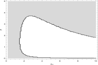
It is rather complicated to precisely describe the set of input parameters that characterizes the order of insider’s certainty equivalents $\left\{(\kappa,p_{I},\lambda)\ |\ \textrm{CE}^{I}_{0-,\iota}\geq\textrm{CE}^{I}_{0-}\right\}$. From Figure 2, we conjugate however that the situation becomes clearer when we consider the asymptotics with respect to traders’ risk tolerances. For this, in the following proposition, we take limits as the insider and uninformed traders’ risk tolerance go to 00 and $\infty$.

Proposition 3.6.

Fix $p_{I},p_{N}$. Then,

  1. (1)

    Fix $\alpha_{I}$. As $\alpha_{U}\to 0$, $\textrm{CE}^{I}_{0-}$ remains bounded while $\textrm{CE}^{I}_{0-,\iota}\to\infty$. As $\alpha_{U}\to\infty$,

    $$\lim_{\alpha_{U}\to\infty}\left(\textrm{CE}^{I}_{0-,\iota}-\textrm{CE}^{I}_{0-}\right)>0.$$
  2. (2)

    Fix $\alpha_{U}$. As $\alpha_{I}\to 0$, $\lim_{\alpha_{I}\to 0}(\textrm{CE}^{I}_{0-,\iota}-\textrm{CE}^{I}_{0-})/\alpha_{I}=0$ but

    limαI0CE0,ιICE0IαI3=d2(1+pI)2(1+pIαU2pIpN)αU2(αU2pIpN+1+pI).subscriptsubscript𝛼𝐼0subscriptsuperscriptCE𝐼limit-from0𝜄subscriptsuperscriptCE𝐼limit-from0superscriptsubscript𝛼𝐼3𝑑2superscript1subscript𝑝𝐼21subscript𝑝𝐼superscriptsubscript𝛼𝑈2subscript𝑝𝐼subscript𝑝𝑁superscriptsubscript𝛼𝑈2superscriptsubscript𝛼𝑈2subscript𝑝𝐼subscript𝑝𝑁1subscript𝑝𝐼\lim_{\alpha_{I}\to 0}\frac{\textrm{CE}^{I}_{0-,\iota}-\textrm{CE}^{I}_{0-}}{\alpha_{I}^{3}}=\frac{d}{2}\frac{(1+p_{I})^{2}(1+p_{I}-\alpha_{U}^{2}p_{I}p_{N})}{\alpha_{U}^{2}(\alpha_{U}^{2}p_{I}p_{N}+1+p_{I})}.

    Thus, for $\alpha_{I}$ small, $\textrm{CE}^{I}_{0-,\iota}\geq\textrm{CE}^{I}_{0-}$ if and only if $1+p_{I}-\alpha_{U}^{2}p_{I}p_{N}\geq 0$. As $\alpha_{I}\to\infty$,

    $$\lim_{\alpha_{I}\to\infty}\left(\textrm{CE}^{I}_{0-,\iota}-\textrm{CE}^{I}_{0-}\right)>0.$$
  3. (3)

    If $\alpha_{I}=\alpha_{U}$, then $\textrm{CE}^{I}_{0-,\iota}\geq\textrm{CE}^{I}_{0-}$.

Proposition 3.6 implies the risk aversion is a crucial parameter for the certainty equivalents’ comparisons. Indeed, when traders have the same risk aversion internalizing price impact always increases agents’ welfare. On the other hand, fixing $\alpha_{U},p_{N}$, insider welfare may be lower than in the price-taking case when she is very risk averse and the following structure condition holds

(36) $$\alpha_{U}^{2}p_{N}>\frac{1}{p_{I}}+1.$$

For example, this condition holds if the uninformed trader is sufficiently risk tolerant, or/and the noise traders’ demand (approximated by its variance) is sufficiently low.

Welfare in the absence of private information

We conclude our welfare analysis proving that if one turns off the asymmetric information channel, and focuses solely on effects due to internalizing of price impact, then remarkably, insider welfare increases at the interim level. As mentioned above, the situation with no private signal assumes only the insider possesses and exploits her price impact. The other (non-noise) traders act as price takers. This corresponds to when a (large) risk averse agent acts strategically, even when she does not have access to a private signal, and when the uninformed traders represent the mass of all other rational agents who are relatively small (i.e. possess no market power) and who also have no private signal. In sum, we are measuring the effects of assuming heterogeneity, not in information, but in internalization of price impact.

For this, recall from Proposition 1.11 that the no-signal equilibrium corresponds to taking $p_{I}\to 0$. Using the interim welfare formulas in Lemmas D.1 and D.2 in Appendix D, we obtain the associated no-signal equilibrium quantities in the following proposition. To state it, recall $\lambda$ from (17).

Proposition 3.7.

As $p_{I}\to 0$ we obtain the almost sure limits for the insider

$$\begin{split}\lim_{p_{I}\to 0}\textrm{CE}^{I}_{0}(G,Z_{N})&=\textrm{CE}_{nsn}^{I}+\frac{\lambda^{2}}{2\alpha_{I}}Z_{N}^{2},\qquad\lim_{p_{I}\to 0}\textrm{CE}^{I}_{0,\iota}(G,Z_{N})=\textrm{CE}_{nsn}^{I}+\frac{\lambda^{2}}{2(1-\lambda^{2})\alpha_{I}}Z_{N}^{2}.\end{split}$$

Therefore, insider interim welfare always increases when internalizing price impact. For the uninformed agent we obtain almost surely

$$\begin{split}\lim_{p_{I}\to 0}\textrm{CE}^{U}_{0}(H)&=\textrm{CE}_{nsn}^{I}+\frac{\alpha_{U}\lambda^{2}}{2\alpha_{I}^{2}}Z_{N}^{2},\qquad\lim_{p_{I}\to 0}\textrm{CE}^{U}_{0,\iota}(H_{\iota})=\textrm{CE}_{nsn}^{I}+\frac{\alpha_{U}\lambda^{2}}{2\alpha_{I}^{2}(1-\lambda^{2})^{2}}Z_{N}^{2},\end{split}$$

and hence interim welfare also always increases when the insider internalizes price impact.

Remark 3.8.

Two quite surprising consequences stem from the above proposition. First, that the insider’s welfare might be higher in the PT equilibrium is directly attributable to the presence of the private signal, as when there is no private signal, internalization of price impact is always beneficial for the insider. Second, assuming no private signal and that both $I,U$ have the same risk tolerance, which forces $\lambda=1/2$ we have the following almost sure order of interim certainty equivalents

$$\textrm{CE}^{U}_{0,\iota}>\textrm{CE}^{I}_{0,\iota}>\textrm{CE}^{U}_{0}=\textrm{CE}^{I}_{0}.$$

Amazingly, not only it is better for the uninformed agent when the insider internalizes her price impact, the uninformed agent’s welfare actually exceeds that of the insider. We explain the mechanism behind these predictions in the next section.

4. Equilibria Structure

In this section, we analyze and compare the equilibrium quantities (allocation and prices) in order to infer the economic intuition behind the models predictions on the effects of price-impact internalization (“internalization”) and insider’s private signal (“private information”). As will be shown, internalization and private information may have competing affects on the insider’s demand, and hence equilibrium quantities. Broadly, internalization has the effect of dampening the position size, while private information may increase the insider’s equilibrium allocation of risk.

We will compare when the insider (1) takes prices as given versus internalizing price impact, and (2) when the insider has a private signal versus when there is no private signal. This leads to four cases. The first two sections deal with the effect of information asymmetry, starting with the price taking (PT) equilibrium and then moving on to the price impact (PI) equilibrium. The last two sections deal with the effect of price impact internalization, staring when there is no private information, and then considering the private signal case. In each section we compare the equilibrium structure of demands and prices. Throughout we use the notation in (17).

Private information effects when price taking

We start with the PT equilibrium, identifying the effect of the signal on the demands, as well as the price. Using (19), (24), (25) and (28) the insider’s optimal demand functions satisfy

(37) $$\widehat{\psi}_{I}(g,z)-\widehat{\psi}_{ns,I}(z)=\frac{(1-\lambda)(p_{I}-p_{U})}{1+\lambda p_{I}+(1-\lambda)p_{U}}(g-p_{0})-\frac{(1-\lambda)(p_{I}(\lambda p_{I}+(1-\lambda)p_{U})+p_{U})}{p_{I}(1+\lambda p_{I}+(1-\lambda)p_{U})}\frac{z}{\alpha_{I}}.$$

As (23) implies $p_{I}>p_{U}$ we see that (as expected) insider optimal demand relative to the no-signal case is increasing in the signal. By contrast, insider relative demand is decreasing in the noise trader demand.

Another interesting effect concerns the outstanding supply, $\Pi=(\alpha_{I}+\alpha_{U})\widehat{\Pi}=-(\alpha_{I}+\alpha_{U})p_{0}$. At the ex-ante level, the expected demand change is

(38) $$\mathbb{E}\left[\widehat{\psi}_{I}(G,Z_{N})-\widehat{\psi}_{ns,I}(Z_{N})\right]=\frac{(1-\lambda)(p_{I}-p_{U})}{1+\lambda p_{I}+(1-\lambda)p_{U}}\widehat{\Pi}>0,$$

so that on average the insider’s position increases due to the private signal. Intuitively, positive supply means that the insider and the uniformed trader are expected to buy the tradeable asset at the equilibrium and for the insider the presence of private signal means that her estimated variance of the tradeable asset (i.e. its risk) is lower. This increases her demand, implying that ex-ante she is more confident to hold higher part of asset supply.

The private signal’s affect on insider demand is transferred to the equilibrium price, as an increase in the insider’s demand tends to increase the price as well. Indeed, from (24) and (28) we find

$$p(h(g,z))-p_{ns}(z)=\frac{\lambda p_{I}+(1-\lambda)p_{U}}{1+\lambda p_{I}+(1-\lambda)p_{U}}(g-p_{0})+\frac{\lambda[(1-\lambda)(p_{I}-p_{U})-p_{I}(consbp_{I}+(1-\lambda)p_{U})]}{p_{I}(1+\lambda p_{I}+(1-\lambda)p_{U})}\frac{z}{\alpha_{I}}.$$

This shows the equilibrium price is increasing in the signal (the factor in front of $z/\alpha_{I}$ can be positive or negative). At the ex-ante level

(39) $$\mathbb{E}\left[p(h(G,Z_{N}))-p_{ns}(Z_{N})\right]=\frac{\lambda p_{I}+(1-\lambda)p_{U}}{1+\lambda p_{I}+(1-\lambda)p_{U}}\widehat{\Pi}>0.$$

Thus, the presence of the signal increases both the insider’s expected demand and expected equilibrium price. Additionally, the equilibrium clearing condition (4) implies the private signal has the opposite effect on the uniformed trader’s demand131313The uninformed agent sees $Z_{N}$ (through the price) in the no-signal equilibrium, but does not see $Z_{N}$ in the PT equilibrium. Therefore, we are not saying the uninformed agent sees $Z_{N}$ in the PT equilibrium and then adjusts her position accordingly. Rather, we are saying the effect of noise trading in the PT equilibrium is to increase the trade size of the uninformed agent over the no-signal equilibrium.. Summarizing,

The presence of private information in the PT equilibria is expected to increase the insider’s demand and the price and to decrease the uniformed trader’s demand.

Private information effects when internalizing price impact

The effects of private signal on equilibrium prices and demands in the PI equilibrium are similar as in the PT equilibrium. Using (11), Theorem 1.6 and Proposition 1.11 we obtain

$$\begin{split}\widehat{\psi}_{I,\iota}(g,z)-\widehat{\psi}_{ns,\iota,I}(z)&=\frac{p_{I}}{1+2\widehat{y}}(g-p_{0})+\left(\frac{\lambda}{1+\lambda}-\frac{\widehat{y}}{1+2\widehat{y}}\right)\frac{z}{\alpha_{I}}.\end{split}$$

As expected, the insider demand (relative to the no-signal case) is increasing with the private signal. Similarly, by noting the right side of (18) is positive at $y=\lambda/(1-\lambda)$ one can use the arguments in the proof of Proposition 2.4 to show $\widehat{y}>\lambda/(1-\lambda)$ and hence the coefficient in front of $z/\alpha_{I}$ is negative. As in the PT equilibrium, at the ex-ante level the presence of signal increases the insider’s demand because

(40) $$\mathbb{E}\left[\widehat{\psi}_{I,\iota}(G,Z_{N})-\widehat{\psi}_{ns,\iota,I}(Z_{N})\right]=\frac{p_{I}}{1+2\widehat{y}}\widehat{\Pi}.$$

As for the equilibrium prices, using (11), (20) and Proposition 1.11 we obtain

$$\begin{split}p_{\iota}(h_{\iota}(g,z))-p_{ns,\iota}(z)&=\frac{p_{I}\widehat{y}}{(1+p_{I})(1+2\widehat{y})}\left(g-p_{0}\right)+\left(\frac{\widehat{y}(1+\widehat{y})}{(1+p_{I})(1+2\widehat{y})}-\frac{\lambda}{1-\lambda^{2}}\right)\frac{z}{\alpha_{I}}.\end{split}$$

Therefore, due to the increased insider demand, the relative price change is increasing in the signal and outstanding supply. At the ex-ante level

$$\mathbb{E}\left[p_{\iota}(h_{\iota}(G,Z_{N}))-p_{ns,\iota}(Z_{N})\right]=\frac{p_{I}\widehat{y}}{(1+p_{I})(1+2\widehat{y})}\widehat{\Pi},$$

which shows a positive difference. This is the same as in the PT case, and in fact, using (39), along with (31) and (32) we obtain

(41) $$\begin{split}\mathbb{E}\left[p(h(G,Z_{N}))-p_{ns}(Z_{N})\right]-\mathbb{E}\left[p_{\iota}(h_{\iota}(G,Z_{N}))-p_{ns,\iota}(Z_{N})\right]=(m_{g}-m_{g,\iota})\widehat{\Pi}.\end{split}$$

Proposition 2.4 thus implies the expected price change caused by the presence of the private signal is lower when accounting for price impact, consistent with the reduced sensitivity with respect to public signal that internalization yields.

As in the PT equilibrium, market clearing implies the effects of the signal on the uniformed trader’s demand are in thee opposite direction of the insider. Indeed, direct calculation shows

$$\mathbb{E}\left[\widehat{\psi}_{U,\iota}(Z_{N})-\widehat{\psi}_{ns,\iota,U}(Z_{N})\right]=-\frac{p_{I}\lambda}{(1-\lambda)(1+2\widehat{y})}\widehat{\Pi},$$

which means that in contrast to the insider, the uniformed trader’s demand is expected to decease due to price impact. Thus, we may conclude

For both the PT and PI equilibria, the presence of a private signal is expected to increase the insider’s demand and price (albeit with a lower change in the PI equilibrium) and decrease the uniformed trader’s demand.

Price impact internalization effects when there is no information asymmetry

We now turn our attention to the effect of price impact, first assuming absence of private information. According to Proposition 1.11, and recalling that $\psi_{I,0}=\widehat{\Pi}$ we see the trades satisfy

(42) $$\left(\widehat{\psi}_{ns,\iota,I}(z)-\psi_{I,0}\right)=-\frac{\lambda}{1+\lambda}\frac{z}{\alpha_{I}},\qquad\left(\widehat{\psi}_{ns,I}(z)-\psi_{I,0}\right)=-\lambda\frac{z}{\alpha_{I}}.$$

Therefore, internalization of price impact keeps the insider at the same side of the trade as in the non-internalization case, but it reduces the magnitude of the trade. Intuitively, the insider accounts for price impact by taking a smaller position, which in turn changes the equilibrium price. Indeed, we readily get that

(43) $$p_{ns,\iota}(z)-p_{ns}(z)=\frac{\lambda^{3}}{1-\lambda^{2}}\frac{z}{\alpha_{I}}.$$

The above implies that in the PI equilibrium, the insider has a lower demand when compared to the PT equilibrium and obtains a better price (price-impact increases the per-unit price when insider sells and decreases it when she buys). Indeed, positive $z$ means that both insider and uniformed trader sell at equilibrium. In the view of Remark 2.2, positive $z$ makes the insider reveal a higher public signal. This increases the demand of the uniformed trader (covers less of noise demand) and hence the interim effect is an increase in the equilibrium price. Lastly, the uniformed trader’s equilibrium allocations imply the relative trade size

$$\left(\widehat{\psi}_{ns,\iota,U}(z)-\psi_{U,0}\right)=-\frac{\lambda}{1-\lambda^{2}}\frac{z}{\alpha_{I}},\qquad\left(\widehat{\psi}_{ns,U}(z)-\psi_{U,0}\right)=-\lambda\frac{z}{\alpha_{I}}.$$

Therefore, when $z<0$ both the insider and uninformed trader buy the risky asset in each equilibria. However, in the PI equilibrium, the insider reduces her position while the uninformed trader increases it. Conversely, when $z>0$ traders sell the risky asset, with the uniformed trader selling more. In particular, the uninformed increases his volume at a better price-per-unit, due to price impact. In other words, when insider buys the asset, internalization reduces her demand which in turn decreases the price and makes the uniformed trader buys more. Summarizing,

Internalization with no signal results in a lower (resp. higher) equilibrium position for the insider (resp. uniformed trader) at a better price.

Price impact internalization effects when there is information asymmetry

We finally consider the effect of price-impact internalization on equilibrium demands and prices in the presence of private information, which associates with our main case. To simplify the presentation and highlight the key points, we state the results at the expected value level, rather than for each realization.

We have seen that the presence of signal is expected to increase the volume of the insider’s order, while the internalization is expected to decrease it (under no private signal). In other words, price impact and presence of the signal have ex-ante opposite expected effects on the insider’s demand. In particular, using (38), (40), (42) and $\mathbb{E}\left[Z_{N}\right]=0$ we obtain

(44) $$\begin{split}\mathbb{E}\left[\widehat{\psi}_{I,\iota}(G,Z_{N})-\widehat{\psi}_{I}(G,Z_{N})\right]&=\left(\frac{p_{I}}{1+2\widehat{y}}-\frac{(1-\lambda)(p_{I}-p_{U})}{1+\lambda p_{I}+(1-\lambda)p_{U}}\right)\widehat{\Pi},\\ &=p_{I}\left(\frac{1}{1+2\widehat{y}}-\frac{(1-\lambda)}{1+\lambda p_{I}+\kappa p_{I}(1+p_{I})}\right)\widehat{\Pi},\end{split}$$

where the second equality follows using (29) and simplifying. The following shows the right side above may be either positive or negative. In short, the effect of price impact prevails over the one of asymmetric information when the insider is sufficiently risk tolerant resulting is a higher expected order.

Proposition 4.1.

The quantity in (44) is positive as $\alpha_{I}\to\infty$ and negative as $\alpha_{I}\to 0$. Therefore, price impact internalization is expected to increase (resp. decrease) the insider’s position when she is sufficiently risk tolerant (resp. risk averse). By market clearing, the opposite is expected for the uninformed trader.

Remark 4.2.

By inspecting the proof of Proposition 4.1 we can identify other instances when $\mathbb{E}\left[\widehat{\psi}_{I,\iota}(G,Z_{N})-\widehat{\psi}_{I}(G,Z_{N})\right]$ is positive or negative. For example, with other parameters fixed, it is positive as (i) $p_{I}\to\infty$, or (ii) as $\alpha_{U}\to 0,\infty$ if $\alpha_{I}^{2}p_{I}p_{N}$ is sufficiently large. Conversely, it is negative as (i) $p_{I}\to 0$ or (ii) as $\alpha_{U}\to 0,\infty$ if $\alpha_{I}^{2}p_{I}p_{N}$ is sufficiently small.

Lastly, for the equilibrium prices, (41), (43) and $\mathbb{E}\left[Z_{N}\right]=0$ give

$$\mathbb{E}\left[p_{\iota}(H_{\iota})-p(H)\right]=(m_{g,\iota}-m_{g})\widehat{\Pi}.$$

Proposition 2.4 implies the right side above is negative, which means that internalization is expected to decrease (resp. increase) the price when insider is expected to buy (resp. sell). In other words, the expected change of the price benefits both traders (as the uniformed trader remains at the same side of trade). Connecting this fact to the expected demand changes, we may conclude that

Due to internalization of price impact, a sufficiently low (resp. high) risk tolerant insider is expected to buy less (resp. more) units at a better price, while uniformed trader buys more (resp. less).


Intuition and model’s predictions

We conclude by providing economic intuition about the predictions induced by the model. First, we have seen that asymmetric information is ex-ante expected to increase the insider’s demand for the tradeable asset. Intuitively, the private signal reduces the asset’s risk (measured by variance) for the insider, which makes her willing to hold a higher allocation. Without strategic trading, higher insider demand is expected to increase the price. Private information tends to increase the insider’s demand even under price impact. The main ex-ante expected difference is the lower increase of the price, as internalization of price impact affects the price in favor of the insider. When the insider trades strategically, she uses her private signal to affect the equilibrium. In fact, it is exactly when the insider internalizes price impact and uninformed agents are price-takers that insider’s welfare is monotonically increasing with respect to the signal precision. In other words, insider’s strategic trading increases the value of her private signal making the acquisition of better signal reasonable.

Internalization of price impact keeps the traders at the same side of trade. As we have seen, the insider hides part of her private signal, which is expected to reduce her demand and hence the equilibrium price. In other words, price impact has the opposite expected effect than the private signal. Provided that insider has long position at equilibrium, the price always decreases due to price impact, under both price impact and private signal. However, the insider’s demand is lower under the presence of signal when she is also sufficiently risk averse. This is intuitive in the sense that a sufficiently risk averse trader wants to undertake less risk. If in addition to high insider’s risk aversion inequality (36) holds, the price impact equilibrium lowers the insider’s welfare. Note that (36) implies the uniformed traders are highly risk tolerant. This reduces the insider’s allocation even further, since the uniformed traders’ demand is higher and hence at market-clearing the insider’s share is lower. Such lower insider’s demand may lead to lower ex-ante expected utility gains, as a signal of good quality (consistent with (36)) means the insider feels more confident to hold a higher position at equilibrium. However, under a large deviation of risk aversions, internalization of price impact prevails, demand is reduced and utility gains are lower. Note that when traders have the same risk aversion, the effect of internalization is always beneficial for the insider.

Interestingly enough, in the absence of a private signal, internalization of price impact induces higher utility gains for the insider. This is because under symmetric information, the insider does not have motive to increase her demand due to a lower asset risk, and hence the effect of price impact, i.e. buying lower quantity at a lower price, increases the expected welfare. We conclude that it is the presence of asymmetric information and the deviation on risk aversions that potentially make the price-impact equilibrium disadvantageous for the insider.

We should also emphasize that as long as the insider internalizes her price impact, equilibrium prices cannot be driven to the corresponding PT equilibrium. This is because the uniformed trader, although he is a price-taker, realizes the insider internalizes her price impact. This makes him reduce his perceived public signal precision, and hence alters his demand function to a less elastic one. Under the Pareto initial allocation, he remains at the same side of trade with the insider and the lower equilibrium prices caused by the internalization imply higher demand for the uniformed trader, who (although price-taker) is benefited by price impact. In other words, price impact decreases the price when traders buy the asset, and at equilibrium the uniformed trader satisfies his optimal demand but at a discount. This is the reason why price impact ex-ante benefits the uniformed trader with and without asymmetric information.

References

  • Anthropelos and Kardaras [2024] M. Anthropelos and C. Kardaras. Price impact under heterogeneous beliefs and restricted participation. Journal of Economic Theory, 215:105774, 2024. ISSN 0022-0531.
  • Back [1992] K. Back. Insider trading in continuous time. Review of Financial Studies, 5(3):387–409, 1992.
  • Benzi and Viviani [2023] Michele Benzi and Milo Viviani. Solving cubic matrix equations arising in conservative dynamics. Vietnam Journal of Mathematics, 51(1):113–126, 2023.
  • Bergemann et al. [2021] D. Bergemann, T. Heumann, and S. Morris. Information, market power, and price volatility. The RAND Journal of Economics, 52(1):125–150, 2021.
  • Goldstein et al. [2023] I. Goldstein, Y. Xiong, and L. Yang. Information sharing in financial markets. Available at SSRN 3632315, 2023.
  • Gong et al. [2022] A. Gong, S. Ke, Y. Qiu, and R. Shen. Robust pricing under strategic trading. Journal of Economic Theory, 199:105201, 2022. Symposium Issue on Ambiguity, Robustness, and Model Uncertainty.
  • Grossman [1976] S. Grossman. On the efficiency of competitive stock markets where trades have diverse information. Journal of Finance, 31(2):573–585, 1976.
  • Grossman and Stiglitz [1980] S.J. Grossman and J.E. Stiglitz. On the impossibility of informationally efficient markets. American Economic Review, 70(3):393–408, 1980.
  • Hellwig [1980] M.F. Hellwig. On the aggregation of information in competitive markets. Journal of Economic Theory, 22(3):477–498, 1980.
  • Hirshleifer [1971] J. Hirshleifer. The private and social value of information and the reward to inventive activity. American Economic Review, 61(2):561––574, 1971.
  • Indjejikian et al. [2014] R. Indjejikian, H. Lu, and L. Yang. Rational information leakage. Management Science, 60(11):2762–2775, 2014.
  • Kacperczyk and Pagnotta [2019] M. T. Kacperczyk and E.S. Pagnotta. Chasing Private Information. The Review of Financial Studies, 32(12):4997–5047, 03 2019.
  • Kacperczyk et al. [2023] M. T. Kacperczyk, J. Nosal, and S. Sundaresan. Market power and price informativeness. Available at SSRN 3137803, 2023.
  • Koijen and Yogo [2019] R.S.J. Koijen and M. Yogo. A demand system approach to asset pricing. Journal of Political Economy, 127(4):1475–1515, 2019.
  • Kovalenkov and Vives [2014a] A. Kovalenkov and V. Vives. Competitive rational expectations equilibria without apology. Journal of Economic Theory, 149:211–235, 2014a.
  • Kovalenkov and Vives [2014b] Alexander Kovalenkov and Xavier Vives. Competitive rational expectations equilibria without apology. Journal of Economic Theory, 149:211–235, 2014b. ISSN 0022-0531. doi: https://doi.org/10.1016/j.jet.2013.05.002. URL https://www.sciencedirect.com/science/article/pii/S0022053113001026. Financial Economics.
  • Kyle [1985] A.S. Kyle. Continuous auctions and insider trading. Econometrica, pages 1315–1335, 1985.
  • Kyle [1989] A.S. Kyle. Informed speculation with imperfect competition. The Review of Economic Studies, 56(3):317–355, 1989.
  • Laffont [1985] J.-J. Laffont. On the welfare analysis of rational expectations equilibria with asymmetric information. Econometrica, 53(1):1–30, 1985.
  • Lou and Rahi [2023] Y. Lou and R. Rahi. Information, market power and welfare. Journal of Economic Theory, 214:105756, 2023.
  • Malamud and Rostek [2017] S. Malamud and M. Rostek. Decentralized exchange. American Economic Review, 107(11):3320–62, 2017.
  • Morris and Shin [2002] S. Morris and H. S. Shin. Social value of public information. American Economic Review, 92(5):1521–1534, December 2002.
  • Nezafat and Schroder [2023] M. Nezafat and M. Schroder. The negative value of private information in illiquid markets. Journal of Economic Theory, 210:105664, 2023.
  • Rochet and Vila [1994] J.-C. Rochet and J.-L. Vila. Insider Trading without Normality. The Review of Economic Studies, 61(1):131–152, 01 1994. ISSN 0034-6527. doi: 10.2307/2297880. URL https://doi.org/10.2307/2297880.
  • Rostek and Weretka [2012] M. Rostek and M. Weretka. Price inference in small markets. Econometrica, 80(2):687–711, 2012.
  • Rostek and Weretka [2015a] M. Rostek and M. Weretka. Dynamic thin markets. Review of Financial Studies, 28:2946–2992, 2015a.
  • Rostek and Weretka [2015b] M. Rostek and M. Weretka. Information and strategic behavior. Journal of Economic Theory, 158:536–557, 2015b. Symposium on Information, Coordination, and Market Frictions.
  • Rostek and Yoon [2023] M. Rostek and J. H. Yoon. Equilibrium theory of financial markets: Recent developments. Prepared for The Journal of Economic Literature, 2023.
  • Spiegel and Subrahmanyam [1992] M. Spiegel and A. Subrahmanyam. Informed speculation and hedging in a noncompetitive securities market. The Review of Financial Studies, 5(2):307–329, 1992.
  • Subrahmanyam [1991] A. Subrahmanyam. Risk aversion, market liquidity, and price efficiency. The Review of Financial Studies, 4(3):417–441, 1991.
  • Vayanos [1999] D. Vayanos. Strategic Trading and Welfare in a Dynamic Market. The Review of Economic Studies, 66(2):219–254, 04 1999.
  • Vayanos [2001] D. Vayanos. Strategic trading in a dynamic noisy market. The Journal of Finance, 56(1):131–171, 2001.
  • Vives [2011] X. Vives. Strategic supply function competition with private information. Econometrica, 79:1919–1966, 2011.
  • Vives [2014] X. Vives. On the possibility of informationally efficient markets. Journal of the European Economic Association, 12(5):1200–1239, 2014.

Appendix A The Equilibrium: General Case

We extend the model of Section 1 to $d$ risky assets with general values for the model inputs, outstanding supply, and agent initial endowments. The assets have terminal payoff $X\sim N(\mu_{X},P_{X}^{-1})$, written

$$X=\mu_{X}+P_{X}^{-1/2}\mathcal{E}_{X},$$

where $\mathcal{E}_{X}\sim N(0,1_{d})$. The outstanding supply is $\Pi\in{\mathbb{R}}^{d}$. The riskless asset price is still normalized to $1$. The private signal $G$ takes the form

(45) $$G=X+Z_{I};\qquad Z_{I}=P_{I}^{-1/2}\mathcal{E}_{I},$$

where $\mathcal{E}_{I}\sim N(0,1_{d})$ is independent of $X$, so that $P_{I}$ is the signal precision matrix. The noise traders have demand

$$Z_{N}=P_{N}^{-1/2}\mathcal{E}_{N},$$

where $\mathcal{E}_{n}\sim N(0,1_{d})$ is independent of both $X$ and $\mathcal{E}_{I}$. The matrices $P_{X},P_{I},P_{N}$ lie in $\mathbb{S}^{d}_{++}$, the set of $d\times d$ strictly positive definite symmetric matrices, and $\mu_{X}\in\mathbb{R}^{d}$. Lastly, the insider $I$ and uninformed agent $U$ are endowed with share positions $\left\{\pi_{i,0}\right\}$ consistent with equilibrium in that (with $\pi_{i,0}=\alpha_{i}\psi_{i,0}$) $\Pi=\alpha_{I}\psi_{I,0}+\alpha_{U}\psi_{U,0}$.

For a given strategy $\pi_{i}$, if the time 00 price vector is $p$ then agent $i$ has risk aversion adjusted terminal wealth (see (5))

(46) $$\mathcal{W}^{\psi_{i}}=(\psi_{i,0})^{\prime}p+\psi_{i}^{\prime}(X-p);\qquad i\in\left\{I,U\right\}.$$

where the symbol denotes transposition. The insider perceives linear price impact so that if she changes her position from $\pi_{I,0}=\alpha_{I}\widehat{\Pi}$ to $\pi_{I}=\alpha_{I}\psi_{I}$, the price will be as in (6) (for a to-be-determined vector $V$ and matrix $M$). The set of acceptable strategies for the insider ${\mathcal{A}}_{I}$ is the same as in (7) and the insider’s optimal investment problem is

(47) $$\begin{split}&\inf_{\psi\in{\mathcal{A}}_{I}}\mathbb{E}\left[e^{-\left(\psi_{I,0}^{\prime}p_{\iota}\left(\psi,Z_{N}\right)+\psi^{\prime}\left(X-p_{\iota}\left(\psi,Z_{N}\right)\right)\right)}\big{|}\sigma(G,Z_{N})\right].\end{split}$$

Write $P_{X|G}$ as the precision of $X$ given the insider signal $G$, and similarly to (9) express $M$ in terms of $P_{X|G}$ and a to-be-determined matrix ${\mathcal{Y}}$.

(48) $$\begin{split}P_{X|G}:=P_{I}+P_{X};\qquad M=M({\mathcal{Y}})=P_{X|G}^{-1/2}\ {\mathcal{Y}}\ P_{X|G}^{-1/2}.\end{split}$$

We also write $V=V({\mathcal{Y}})$ to stress the dependence, and expect ${\mathcal{Y}}+{\mathcal{Y}}^{\prime}\in\mathbb{S}^{d}_{++}$. Analogously to Lemma 1.1 we obtain a unique solution to the insider’s optimal investment problem

Lemma A.1.

Let $g,z\in\mathbb{R}$. On the set $\left\{G=g,Z_{N}=z\right\}$, the unique optimizer of (47) enforces

(49) $$\begin{split}\widehat{\psi}_{I,\iota}(g,z)-\psi_{I,0}+\frac{z}{\alpha_{I}}&={\mathcal{M}}\left(g+\Lambda_{\iota}z+\mathcal{V}\right),\end{split}$$

where

(50) $$\begin{split}{\mathcal{M}}={\mathcal{M}}({\mathcal{Y}})&:=P_{X|G}^{1/2}(1_{d}+{\mathcal{Y}}+{\mathcal{Y}}^{\prime})^{-1}P_{X|G}^{-1/2}P_{I},\\ \Lambda_{\iota}=\Lambda_{\iota}({\mathcal{Y}})&:=\frac{1}{\alpha_{I}}P_{I}^{-1}P_{X|G}^{1/2}(1_{d}+{\mathcal{Y}}^{\prime})P_{X|G}^{-1/2},\\ \mathcal{V}=\mathcal{V}({\mathcal{Y}})&:=P_{I}^{-1}\left(P_{X}\mu_{X}-\psi_{I,0}-P_{X|G}V({\mathcal{Y}})\right).\end{split}$$

Motivated by (49) we define the market signal and its precision

(51) $$\begin{split}H_{\iota}&:=G+\Lambda_{\iota}Z_{N}=X+Z_{I}+\Lambda_{\iota}Z_{N},\\ P_{U,\iota}&=P_{U,\iota}({\mathcal{Y}}):=\left(P_{I}^{-1}+\Lambda_{\iota}({\mathcal{Y}})P_{N}^{-1}\Lambda_{\iota}^{\prime}({\mathcal{Y}})\right)^{-1}.\end{split}$$

By observing the price, the uniformed trader has time 00 information $\sigma(H_{\iota})$ and written as a function of $H_{\iota}$, the price is $p(H_{\iota})$ where

(52) $$\begin{split}p_{\iota}(h_{\iota})&=M{\mathcal{M}}(h_{\iota}+\mathcal{V})+V.\end{split}$$

As the uninformed is a price taker, his optimization problem is

$$\begin{split}&\inf_{\psi\in\sigma(H_{\iota})}\mathbb{E}\left[e^{-\left(\psi_{U,0}^{\prime}p_{\iota}\left(H_{\iota}\right)+\psi^{\prime}\left(X-p_{\iota}\left(H_{\iota}\right)\right)\right)}\big{|}\sigma(H_{\iota})\right].\end{split}$$

Similarly to Lemma A.1 we obtain

Lemma A.2.

Let $h_{\iota}\in\mathbb{R}$. On the set $\left\{H_{\iota}=h_{\iota}\right\}$, the uninformed agent has risk-aversion adjusted optimal demand

(53) $$\widehat{\psi}_{U,\iota}(h_{\iota})=P_{U,\iota}h_{\iota}+P_{X}\mu_{X}-(P_{U,\iota}+P_{X})p_{\iota}(h_{\iota}).$$

The market-clearing condition is

(54) $$\begin{split}\Pi&=\alpha_{I}\left(\widehat{\psi}_{I,\iota}(G,Z_{N})-\psi_{I,0}+\frac{Z_{N}}{\alpha_{I}}\right)+\alpha_{I}\psi_{I,0}+\alpha_{U}\widehat{\psi}_{U,\iota}(H_{\iota}).\end{split}$$

Taking into account (49), (50) and (53), the above will induce the equilibrium conditions on ${\mathcal{Y}}$ and $V$, as stated in the next proposition. To state it, as in (19) but for the general setup, define

(55) $$p_{0}:=\mathbb{E}^{{\mathbb{Q}}_{0}}\left[X\right]=\mu_{X}-P_{X}^{-1}\widehat{\Pi}.$$

As before, $p_{0}$ is the equilibrium price absent any private signals, and provided the initial endowments satisfy (2).

Proposition A.3.

Assume $\widehat{{\mathcal{Y}}}$ enforces the matrix equality

(56) $$\begin{split}0_{d}&=P_{U,\iota}(\widehat{{\mathcal{Y}}}){\mathcal{M}}({\mathcal{Y}})^{-1}+\frac{\alpha_{I}}{\alpha_{U}}1_{d}-(P_{U,\iota}(\widehat{{\mathcal{Y}}})+P_{X})M(\widehat{{\mathcal{Y}}}),\end{split}$$

where $M$, ${\mathcal{M}}$ and $P_{U,\iota}$ are from (48), (50) and (51). Then, there exists a price-impact equilibrium. The market signal is $H_{\iota}$ from (51), and the equilibrium price $p_{\iota}$ is of the form (52) with $M=M(\widehat{{\mathcal{Y}}})$ from (48), and

(57) $$V=V(\widehat{{\mathcal{Y}}})=p_{0}+P_{X}^{-1}P_{\iota}(\widehat{{\mathcal{Y}}})(P_{I}-P_{\iota}(\widehat{{\mathcal{Y}}}))^{-1}\left(\psi_{I,0}-\widehat{\Pi}\right);\qquad P_{\iota}(\widehat{{\mathcal{Y}}}):=\frac{\alpha_{I}P_{I}+\alpha_{U}P_{U,\iota}(\widehat{{\mathcal{Y}}})}{\alpha_{I}+\alpha_{U}}.$$

Lastly, the price function $p_{\iota}$ takes the form

(58) $$\begin{split}p_{\iota}(h_{\iota})&=p_{0}+M(\widehat{{\mathcal{Y}}}){\mathcal{M}}(\widehat{{\mathcal{Y}}})\left(h_{\iota}-p_{0}\right)\\ &\quad+\left(P_{X}^{-1}-M(\widehat{{\mathcal{Y}}}){\mathcal{M}}(\widehat{{\mathcal{Y}}})\left(P_{\iota}(\widehat{{\mathcal{Y}}})^{-1}+P_{X}^{-1}\right)\right)P_{\iota}(\widehat{{\mathcal{Y}}})(P_{I}-P_{\iota}(\widehat{{\mathcal{Y}}}))^{-1}\left(\psi_{I,0}-\widehat{\Pi}\right).\end{split}$$

In light of Proposition A.3, our goal is to find solutions $\widehat{{\mathcal{Y}}}$ to (56). This is a matrix-valued cubic equation for ${\mathcal{Y}}$ and the primary difficulty in establishing existence of solutions $\widehat{{\mathcal{Y}}}$ arises due to the interaction between the precision matrices $P_{I},P_{N}$ and $P_{X}$. While techniques exist for solving such equations (see Benzi and Viviani [2023]), technically this would take us far beyond the intended scope of the paper, and therefore we make the following assumption, which is always valid in the case of a single asset (as in our simplified model of Section 1).

Assumption A.4.

$P_{I}=p_{I}P_{X}$ and $P_{N}=p_{N}P^{-1}_{X}$ for scalars $p_{I},p_{N}>0$.

Under this assumption we guess that ${\mathcal{Y}}=y1_{d}$ for a scalar $y>0$. The quantities in (48), (50) and (51) take the form

(59) $$\begin{split}M&=\frac{y}{1+p_{I}}P_{X}^{-1},\quad{\mathcal{M}}=\frac{p_{I}}{1+2y}P_{X},\quad\Lambda_{\iota}=\frac{y+1}{\alpha_{I}p_{I}}P_{X}^{-1},\quad P_{U,\iota}=\left(\frac{\alpha_{I}^{2}p_{I}^{2}p_{N}}{(1+y)^{2}+\alpha_{I}^{2}p_{I}p_{N}}\right)P_{X}.\end{split}$$

Note the constant in front of $P_{U,\iota}$ is exactly (13). Plugging these values and simplifying one can show that (56) holds if and only if $y$ solves (18). Therefore, using Proposition 1.5 we obtain the following generalization of Theorem 1.6.

Theorem A.5.

Let Assumption A.4 hold. Then a price-impact equilibrium exists. Using $\widehat{y}$ from Proposition 1.5, the market signal is $H_{\iota}$ from (51). The equilibrium price is $p_{\iota}(H_{\iota})$ for $p_{\iota}$ from (58). The insider uses the optimal policy $\widehat{\pi}_{I,\iota}=(1/\alpha_{I})\widehat{\psi}_{I,\iota}(G,Z_{N})$ from (49). The uninformed agent uses the optimal policy $\widehat{\pi}_{U,\iota}=(1/\alpha_{U})\widehat{\psi}_{U,\iota}(H)$ for $\widehat{\psi}_{U,\iota}$ from (53).

Price-taking equilibrium

To state the price taking results, assume there is a market signal $H$ revealed through the time 00 price $p=p(H)$, and both traders take $p(H)$ as given. The insider has time 0 information $\sigma(H,G)$ while the uninformed trader uses $\sigma(H)$. Using (46), the insider and uninformed trader’s optimal investment problems are as in (21), where again $(H,p(H))$ is a price-taking equilibrium if the clearing condition (4) holds for the optimal policies. As this result does not require Assumption A.4 we state it for general parameter values (it generalizes Proposition 1.7).

Proposition A.6.

There is a price-taking equilibrium. The market signal is

(60) $$H:=G+\frac{1}{\alpha_{I}}P_{I}^{-1}Z_{N}=X+Z_{I}+\frac{1}{\alpha_{I}}P_{I}^{-1}Z_{N}.$$

$H$ is of the same form as $G$, but with lower precision

$$P_{U}:=\left(P_{I}^{-1}+\frac{1}{\alpha_{I}^{2}}P_{I}^{-1}P_{N}^{-1}P_{I}^{-1}\right)^{-1}.$$

With $p_{0}$ from (55), the equilibrium price is $p=p(H)$ for the price function

(61) $$\begin{split}p(h)&:=p_{0}+\left(P_{X}+P\right)^{-1}P\left(h-p_{0}\right);\quad P:=\frac{\alpha_{I}P_{I}+\alpha_{U}P_{U}}{\alpha_{I}+\alpha_{U}}.\\ \end{split}$$

The optimal policies for $I$ and $U$ are $\widehat{\psi}_{I}(G,H)$ and $\widehat{\psi}_{U}(H)$ respectively, where

(62) $$\widehat{\psi}_{I}(g,h)=P_{X}\mu_{X}+P_{I}g-(P_{I}+P_{X})p(h);\quad\widehat{\psi}_{U}(h)=P_{X}\mu_{X}+P_{U}h-(P_{U}+P_{X})p(h).$$

No private signal (NS) equilibrium

Continuing, we state the equilibrium results (generalizing Proposition 1.11) where there is no private signal, recalling $\widehat{\Pi}$ and $p_{0}$ from (55).

Proposition A.7.

The no-signal equilibrium corresponds to $p_{I}=0$. In the price-taking case, the equilibrium price and the risk aversion adjusted optimal positions are $p_{ns}(Z_{N})$ and $\widehat{\psi}_{ns,I}=\widehat{\psi}_{ns,U}=\widehat{\psi}_{ns}(Z_{N})$ where

(63) $$p_{ns}(z)=p_{0}+\lambda P_{X}^{-1}\frac{z}{\alpha_{I}};\qquad\widehat{\psi}_{ns}(z)=\widehat{\Pi}-\lambda\frac{z}{\alpha_{I}},$$

where $\lambda$ is defined in (17). In the price-impact case, the equilibrium price is $p_{ns,\iota}(Z_{N})$ where

$$\begin{split}p_{ns,\iota}(z)&=p_{0}+\frac{\lambda}{1-\lambda^{2}}P_{X}^{-1}\frac{z}{\alpha_{I}}+\frac{\lambda^{2}}{1-\lambda^{2}}P_{X}^{-1}\left(\psi_{I,0}-\widehat{\Pi}\right).\end{split}$$

The risk aversion adjusted optimal policies for $I$ and $U$ are $\widehat{\psi}_{ns,\iota,I}(Z_{N})$ and $\widehat{\psi}_{ns,\iota,U}(Z_{N})$, where

$$\begin{split}\widehat{\psi}_{ns,\iota,I}(z)&=\psi_{I,0}-\frac{\lambda}{1+\lambda}\frac{z}{\alpha_{I}}-\frac{1}{1+\lambda}\left(\psi_{I,0}-\widehat{\Pi}\right),\\ \widehat{\psi}_{ns,\iota,U}(z)&=\psi_{I,0}-\frac{\lambda}{1-\lambda^{2}}\frac{z}{\alpha_{I}}-\frac{1}{1-\lambda^{2}}\left(\psi_{I,0}-\widehat{\Pi}\right).\end{split}$$

Appendix B Proofs from Section 1 and Appendix A

Let us first provide a mapping between the results of Section 1 and Section A. First, Lemmas 1.1, 1.3 follow directly from Lemmas A.1, A.2 respectively. Next, while Lemma 1.4 could be deduced from Proposition A.3, the algebra is quite complicated so we will provide a short stand alone proof. Proposition 1.5 requires its own proof. In Theorem 1.6, the statement regarding the price function $p_{\iota}$ follows from Proposition A.3, and that regarding $\widehat{\psi}_{U,\iota}$ follows from Lemma A.2. As for $\widehat{\psi}_{I,\iota}$ we will offer a stand-alone derivation. Lastly, Propositions 1.7, 1.11 follow from Propositions A.6, A.7 respectively. Therefore, we will first provide the necessary proofs from Section 1 and then move on to Appendix A.

Proof of Lemma 1.4.

(16) can be written

$$\begin{split}0&=\alpha_{I}\left(\frac{p_{I}}{1+2y}(h_{\iota}+\widehat{\Pi})-\frac{1+p_{I}}{1+2y}(V(y)+\widehat{\Pi})\right)\\ &\qquad+\alpha_{U}\left(\left(p_{U,\iota}-\frac{(1+p_{U,\iota})p_{I}y}{(1+p_{I})(1+2y)}\right)(h_{\iota}+\widehat{\Pi})-\frac{(1+p_{U,\iota})(1+y)}{1+2y}(V(y)+\widehat{\Pi})\right)\\ &\qquad+\alpha_{U}\left(-1+\frac{(1+p_{U,\iota})y}{(1+p_{I})(1+2y)}-p_{U,\iota}+\frac{(1+p_{U,\iota})p_{I}y}{(1+p_{I})(1+2y)}+\frac{(1+p_{U,\iota})(1+y)}{1+2y}\right)\widehat{\Pi}.\end{split}$$

Direct calculation shows the term on the third line above vanishes, so that if $V(y)=-\widehat{\Pi}$ the clearing condition will hold provided

(64) $$\begin{split}0&=\alpha_{I}\frac{p_{I}}{1+2y}+\alpha_{U}\left(p_{U,\iota}-\frac{(1+p_{U,\iota})p_{I}y}{(1+p_{I})(1+2y)}\right),\\ &=\frac{\alpha_{I}p_{I}}{(1+2y)((1+y)^{2}+\alpha_{I}^{2}p_{I}p_{N}}\left((1+y)^{2}\left(1-\frac{\alpha_{U}y}{\alpha_{I}(1+p_{I})}\right)+\alpha_{I}^{2}p_{I}p_{N}\left(\frac{\alpha_{U}}{\alpha_{I}}y+\frac{\alpha_{U}+\alpha_{I}}{\alpha_{I}}\right)\right).\end{split}$$

Proof of Proposition 1.5.

Define $g(y)$ as the cubic function on the right side of (18). It is clear that $g(0)>0$ and $\lim_{y\to\infty}g(y)=-\infty$. This shows there exists a solution $\widehat{y}>0$ to $g(\widehat{y})=0$. As for uniqueness of positive solutions, straight-forward computations show for any solution to $g(y)=0$ that

$$(1+y)\dot{g}(y)=-\frac{1-\lambda}{\lambda}(1+y)\kappa p_{I}-\kappa p_{I}-(1+y)^{3}\frac{1-\lambda}{\lambda(1+p_{I})}<0.$$

Thus, for any solution $y>-1$, $g$ strictly decreasing at $y$ and hence there is a unique solution exceeding $-1$, which is in fact positive.

Derivation of $\widehat{\psi}_{I,\iota}(g,z)$ in Theorem 1.6.

From (10), (11), $V(y)=\widehat{\Pi}$, (19) and (20) we obtain

$$\begin{split}\widehat{\psi}_{I,\iota}(g,z)&=-p_{0}+\frac{p_{I}}{1+\widehat{y}}(g-h_{\iota})+\frac{p_{I}}{1+2\widehat{y}}(h_{\iota}-p_{0}),\\ &=-\left(1+\frac{p_{I}}{1+\widehat{y}}\right)p_{0}+\frac{p_{I}}{1+\widehat{y}}g-\frac{p_{I}\widehat{y}}{(1+\widehat{y})(1+2\widehat{y})}(h_{\iota}-p_{0}),\\ &=-\left(1+\frac{p_{I}}{1+\widehat{y}}\right)p_{0}+\frac{p_{I}}{1+\widehat{y}}g-\frac{1+p_{I}}{1+\widehat{y}}(p_{\iota}(h_{\iota})-p_{0}),\\ &=\frac{1}{1+\widehat{y}}\left(p_{I}g-(1+p_{I})p_{\iota}(h_{\iota})-\widehat{y}p_{0}\right).\end{split}$$

Above, the third equality used (20).

Proof of Lemma A.1.

The law of $X$ given $\sigma(G,Z_{N})$ has density

(65) $$\frac{\mathbb{P}\left[X\in dx\big{|}\sigma(G,Z_{N})\right]}{\mathbb{P}\left[X\in dx\right]}=\frac{\mathbb{P}\left[X\in dx\big{|}\sigma(G)\right]}{\mathbb{P}\left[X\in dx\right]}=\left(\frac{e^{-\frac{1}{2}x^{\prime}P_{I}x+x^{\prime}P_{I}g}}{\mathbb{E}\left[e^{-\frac{1}{2}X^{\prime}P_{I}X+X^{\prime}P_{I}g}\right]}\right)\bigg{|}_{g=G}.$$

Using this in (47), on $\left\{G=g,Z_{N}=z\right\}$ the insider minimizes over $\psi=\psi(g,z)$ with $\psi(G,Z_{N})\in{\mathcal{A}}_{I}$

$$\begin{split}&(\psi-\psi_{I,0})^{\prime}p_{\iota}\left(\psi,z\right)+\log\left(\frac{\mathbb{E}\left[e^{-\psi^{\prime}X-\frac{1}{2}X^{\prime}P_{I}x+X^{\prime}P_{I}g}\right]}{\mathbb{E}\left[e^{-\frac{1}{2}X^{\prime}P_{I}X+X^{\prime}P_{I}g}\right]}\right).\\ \end{split}$$

As $X\sim N(\mu_{X},P_{X}^{-1})$, this specifies to

$$(\psi-\psi_{I,0})^{\prime}p_{\iota}\left(\psi,z\right)+\frac{1}{2}\psi^{\prime}(P_{I}+P_{X})^{-1}\psi-\psi^{\prime}\left(P_{I}+P_{X}\right)^{-1}\left(P_{I}g+P_{X}\mu_{X}\right).$$

Plugging in for $p_{\iota}$, using $\psi^{\prime}M\psi=(1/2)\psi^{\prime}(M+M^{\prime})\psi$, and grouping by powers of $\psi$ gives

(66) $$\begin{split}&\frac{1}{2}\psi_{I,0}^{\prime}M\left(\psi_{I,0}-\frac{z}{\alpha_{I}}\right)-\psi_{I,0}^{\prime}V+\frac{1}{2}\psi^{\prime}\left(M+M^{\prime}+(P_{I}+P_{X})^{-1}\right)\psi\\ &\qquad-\psi^{\prime}(P_{I}+P_{X})^{-1}\left(P_{I}g+P_{X}\mu_{X}+(P_{I}+P_{X})\left((M+M^{\prime})\psi_{I,0}-M\frac{z}{\alpha_{I}}-V\right)\right).\end{split}$$

Plugging in for $M$ and using $P_{X|G}$ from (48), the optimizer $\widehat{\psi}_{I}$ is

(67) $$\begin{split}\widehat{\psi}_{I,\iota}(g,z)&=P_{X|G}^{1/2}({\mathcal{Y}}+{\mathcal{Y}}^{\prime}+1_{d})^{-1}P_{X|G}^{-1/2}\bigg{(}P_{I}g+P_{X}\mu_{X}-P_{X|G}V+P_{X|G}^{1/2}({\mathcal{Y}}+{\mathcal{Y}}^{\prime})P_{X|G}^{-1/2}\psi_{I,0}\\ &\quad-P_{X|G}^{1/2}{\mathcal{Y}}P_{X|G}^{-1/2}\frac{z}{\alpha_{I}}\bigg{)}.\end{split}$$

The identity in (49) with ${\mathcal{M}},\Lambda_{\iota},\mathcal{V}$ from (50) follow by direct computations. ∎

Proof of Lemma A.2.

As the uninformed is a price taker, this follows immediately from Proposition A.6 below, with the appropriate substitutions $p\to p_{\iota}$, $H\to H_{\iota}$. ∎

Proof of Proposition A.3.

Throughout we suppress the dependence of all quantities on ${\mathcal{Y}}$. Now, (49), (52) and (53) show the right side of (54) is affine in the signal $H_{\iota}$, and after dividing by $\alpha_{U}$ and right-multiplying by ${\mathcal{M}}^{-1}$, (56) is precisely the equation which eliminates the $H_{\iota}$ terms. As for the constant terms, we need

$$\begin{split}\Pi&=\left(\alpha_{I}1_{d}-\alpha_{U}(P_{U,\iota}+P_{X})M\right){\mathcal{M}}\mathcal{V}+\alpha_{I}\psi_{I,0}+\alpha_{U}\left(P_{X}\mu_{X}-(P_{U,\iota}+P_{X})V\right).\end{split}$$

As (56) does not involve $V$, if $\widehat{{\mathcal{Y}}}$ is such that (56) holds, the above becomes

$$\begin{split}\Pi&=-\alpha_{U}P_{U,\iota}\mathcal{V}+\alpha_{I}\psi_{I,0}+\alpha_{U}\left(P_{X}\mu_{X}-(P_{U,\iota}+P_{X})V\right),\\ &=-\alpha_{U}P_{I}^{-1}P_{U,\iota}\left(P_{X}\mu_{X}-\psi_{I,0}-P_{X|G}V\right)+\alpha_{I}\psi_{I,0}+\alpha_{U}\left(P_{X}\mu_{X}-(P_{U,\iota}+P_{X})V\right),\\ &=\alpha_{U}(P_{I}-P_{U,\iota})P_{I}^{-1}P_{X}(\mu_{X}-V)+(\alpha_{I}P_{I}+\alpha_{U}P_{U,\iota})\psi_{I,0},\end{split}$$

where the last equality follows from (50), (48) and simplifying. Therefore, using $\widehat{\Pi}$ and $p_{0}$ from (55), and $P_{\iota}$ from (57) we deduce

$$\begin{split}\widehat{\Pi}&=\frac{\alpha_{U}}{\alpha_{I}+\alpha_{U}}\left(P_{I}-P_{U,\iota}\right)P_{I}^{-1}P_{X}\left(\mu_{X}-V\right)+\frac{\alpha_{U}P_{U,\iota}+\alpha_{I}P_{I}}{\alpha_{I}+\alpha_{U}}P_{I}^{-1}\psi_{I,0},\\ &=\left(P_{I}-P_{\iota}\right)P_{I}^{-1}P_{X}\left(p_{0}-V\right)+\left(P_{I}-P_{\iota}\right)P_{I}^{-1}\widehat{\Pi}+P_{\iota}P_{I}^{-1}\psi_{I,0}.\end{split}$$

This yields

$$V=p_{0}+P_{X}^{-1}P_{I}\left(P_{I}-P_{\iota}\right)^{-1}P_{\iota}P_{I}^{-1}\left(\psi_{I,0}-\widehat{\Pi}\right).$$

(57) now follows as $P_{I}(P_{I}-P_{\iota})^{-1}P_{\iota}P_{I}^{-1}=P_{\iota}(P_{I}-P_{\iota})^{-1}$. As for (58), we have from (52) that

$$p_{\iota}(h_{\iota})=p_{0}+M{\mathcal{M}}(h_{\iota}-p_{0})+\left(M{\mathcal{M}}-1_{d}\right)p_{0}+M{\mathcal{M}}\mathcal{V}+V.$$

Next,

$$\begin{split}&\left(M{\mathcal{M}}-1_{d}\right)p_{0}+M{\mathcal{M}}\mathcal{V}+V\\ &\qquad=\left(M{\mathcal{M}}-1_{d}\right)p_{0}+V+M{\mathcal{M}}P_{I}^{-1}\left(P_{X}p_{0}+\widehat{\Pi}-\psi_{I,0}-P_{X|G}V\right),\\ &\qquad=\left(M{\mathcal{M}}-1_{d}\right)p_{0}+p_{0}+P_{X}^{-1}P_{\iota}(P_{I}-P_{\iota})^{-1}\left(\psi_{I,0}-\widehat{\Pi}\right)\\ &\qquad\qquad+M{\mathcal{M}}P_{I}^{-1}\left(P_{X}p_{0}-\left(\psi_{I,0}-\widehat{\Pi}\right)-P_{X|G}p_{0}-P_{X|G}P_{X}^{-1}P_{\iota}(P_{I}-P_{\iota})^{-1}\left(\psi_{I,0}-\widehat{\Pi}\right)\right).\end{split}$$

Because $P_{X|G}=P_{I}+P_{X}$ the $p_{0}$ terms cancel out. The $\psi_{I,0}-\widehat{\Pi}$ terms are

$$\begin{split}&-M{\mathcal{M}}P_{I}^{-1}+\left(1_{d}-M{\mathcal{M}}P_{I}^{-1}(P_{X}+P_{I})\right)P_{X}^{-1}P_{\iota}(P_{I}-P_{\iota})^{-1}\\ &\qquad=\left(P_{X}^{-1}-M{\mathcal{M}}(P_{\iota}^{-1}+P_{X}^{-1})\right)P_{\iota}(P_{I}-P_{\iota})^{-1}.\end{split}$$

Proof of Proposition A.6.

Assume the market signal takes the form $H=G+\Lambda Z_{N}$, for a to-be-determined matrix $\Lambda$, and the time 00 price is a function $p=p(H)$ of the market signal. Clearly, $\sigma(G,H)=\sigma(G,Z_{N})$, and hence (21) is equivalent to

$$\begin{split}&\inf_{\psi\in\sigma(G,Z_{N})}\mathbb{E}\left[e^{-\psi_{I,0}^{\prime}p(H)-\psi^{\prime}\left(X-p(H)\right)}\big{|}\sigma(G,Z_{N})\right].\end{split}$$

We may ignore the $\psi_{I,0}^{\prime}p(H)$ term, and using (65), on the set $\left\{G,H\right\}=\left\{g,h\right\}$ the insider solves

$$\inf_{\psi}\left(\psi^{\prime}p(h)+\log\left(\frac{\mathbb{E}\left[e^{-\psi^{\prime}X-\frac{1}{2}X^{\prime}P_{I}X+X^{\prime}P_{I}g}\right]}{\mathbb{E}\left[e^{-\frac{1}{2}X^{\prime}P_{I}X+X^{\prime}P_{I}g}\right]}\right)\right).$$

Using that $X\sim N(\mu_{X},P_{X}^{-1})$, this problem is equivalent to minimizing

$$\frac{1}{2}\psi_{I}^{\prime}(P_{I}+P_{X})^{-1}\psi_{I}-\psi_{I}^{\prime}(P_{I}+P_{X})^{-1}\left(P_{X}\mu_{X}+P_{I}g-(P_{I}+P_{X})p(h)\right),$$

which yields $\widehat{\psi}_{I}$ from (62). Next, the clearing condition (4) mandates that $\widehat{\psi}_{I}+Z_{N}/\alpha_{I}$ be $\sigma(H)$ measurable in equilibrium. Using (62), this in turn implies

$$\widehat{\psi}_{I}(G,H)+\frac{Z_{N}}{\alpha_{I}}=P_{I}\left(G+\frac{1}{\alpha_{I}}P_{I}^{-1}Z_{N}\right)+P_{X}\mu_{X}-(P_{I}+P_{X})p(H),$$

must be $\sigma(H)$ measurable, which is achieved setting $H$ as in (60). Turning to $U$, as $H$ is of the same form as $G$, we may repeat the steps for the insider, but using $(P_{U},H)$ rather than $(P_{I},G)$, to conclude that $\widehat{\psi}_{U}$ as in (62) is optimal. We now use (4) to identify $p(H)$. Indeed, in equilibrium we must have

$$\Pi=\alpha_{I}\left(\widehat{\psi}_{I}(G,H)+\frac{Z_{N}}{\alpha_{I}}\right)+\alpha_{U}\widehat{\psi}_{U}(H),$$

which, using $\widehat{\Pi}$ from (2) and $P$ from (61), implies

$$\begin{split}\widehat{\Pi}&=\frac{\alpha_{I}}{\alpha_{I}+\alpha_{U}}\left(P_{I}H+p_{X}\mu_{X}-(P_{I}+P_{X})p(H)\right)+\frac{\alpha_{U}}{\alpha_{I}+\alpha_{U}}\left(P_{U}H+p_{X}\mu_{X}-(P_{U}+P_{X})p(H)\right),\\ &=PH+P_{X}\mu_{X}-(P_{X}+P)p(H).\end{split}$$

Therefore, using (2) again, $p(H)=(P_{X}+P)^{-1}\left(PH+P_{X}p_{0}\right)$ which gives (61), finishing the result.

The proof of Proposition A.7, as well as those in both Sections C and D simplify if we adjust the notation in (17) by defining

(68) $$\beta:=\kappa p_{I}=\alpha_{I}^{2}p_{I}p_{N};\quad\lambda_{I}:=\lambda=\frac{\alpha_{I}}{\alpha_{I}+\alpha_{U}};\quad\lambda_{U}:=1-\lambda=\frac{\alpha_{U}}{\alpha_{I}+\alpha_{U}},\quad R:=\frac{1}{1+p_{I}}.$$

The cubic equation (18) becomes

(69) $$0=(1+y)^{2}\left(1-\frac{\lambda_{U}R}{\lambda_{I}}y\right)+\beta\left(\frac{\lambda_{U}}{\lambda_{I}}(1+y)+1\right).$$

Next, recall that in the general setup of Appendix A

(70) $$X=\mu_{X}+P_{X}^{-1/2}\mathcal{E}_{X};\quad G=X+\frac{1}{\sqrt{p_{I}}}P_{X}^{-1/2}\mathcal{E}_{I};\qquad Z_{N}=\frac{1}{\sqrt{p_{N}}}P_{X}^{1/2}\mathcal{E}_{N},$$

where $\mathcal{E}_{X},\mathcal{E}_{I},\mathcal{E}_{N}$ are three independent $N(0,1_{d})$ random variables.

Proof of Proposition A.7.

We use the notation in (68), and suppress $\widehat{y}$ from the $M,{\mathcal{M}},\mathcal{V},V$ functions. We start with the price taking equilibria. From (45), (60), (68), as well as the general pricing formulas in (73) below we obtain after some computation

$$\begin{split}p(H)&=p_{0}+\frac{\beta+\lambda_{I}}{\lambda_{U}R+\beta+\lambda_{I}}\left((1-R)X+\sqrt{R(1-R)}P_{X}^{-1/2}\mathcal{E}_{I}+\frac{1}{\alpha_{I}}RP_{X}^{-1}Z_{N}-(1-R)p_{0}\right).\end{split}$$

In (68) note that $p_{I}\to 0$ corresponds to $R\to 1,\beta\to 0$. Therefore, almost surely

$$\begin{split}\lim_{p_{I}\to 0}p(H)&=p_{0}+\frac{\lambda_{I}}{(\lambda_{U}+\lambda_{I})}P_{X}^{-1}\frac{Z_{N}}{\alpha_{I}}=p_{0}+\lambda_{I}P_{X}^{-1}\frac{Z_{N}}{\alpha_{I}},\end{split}$$

because $\lambda_{U}+\lambda_{I}=1$. This gives the pricing formula in (63) as $\lambda=\lambda_{I}$. As for the positions, first note from (72) below that

$$\begin{split}P_{U}&=\frac{(1-R)\beta}{R(1+\beta)}P_{X}\to 0;\qquad P_{I}G=\frac{1-R}{R}P_{X}\left(X+\sqrt{\frac{R}{1-R}}P_{X}^{-1/2}{\mathcal{E}}_{I}\right)\to 0,\\ P_{U}H&=\frac{(1-R)\beta}{R(1+\beta)}P_{X}\left(X+\sqrt{\frac{R}{1-R}}P_{X}^{-1/2}\mathcal{E}_{I}+\frac{R}{\alpha_{I}(1-R)}P_{X}^{-1}Z_{N}\right)\to 0.\end{split}$$

(63) follows from (55) and (62). We next consider the price impact case. From (68) and (69) we see that $p_{I}\to 0$ additionally implies $(1-R)/p_{I}\to 1$ and $\widehat{y}\to\lambda_{I}/\lambda_{U}$. From (45), (51), and (73)

$$\begin{split}p_{\iota}(H_{\iota})&=p_{0}+\frac{\widehat{y}}{1+2\widehat{y}}\times\left((1-R)X+\sqrt{R(1-R)}P_{X}^{-1/2}\mathcal{E}_{I}+\frac{R(1+\widehat{y})}{\alpha_{I}}P_{X}^{-1}Z_{N}-(1-R)p_{0}\right)\\ &\qquad+\frac{\lambda_{I}\widehat{y}\left(\beta+(1+\widehat{y})^{2}\right)}{\lambda_{U}(1+2\widehat{y})(1+\widehat{y})^{2}}\times P_{X}^{-1}\left(\psi_{I,0}-\widehat{\Pi}\right).\end{split}$$

Therefore, almost surely, and using $\lambda_{U}+\lambda_{I}=1$

$$\begin{split}\lim_{p_{I}\to 0}p_{\iota}(H_{\iota})&=p_{0}+\frac{\lambda_{I}(\lambda_{U}+\lambda_{I})}{(\lambda_{U}+2\lambda_{I})\lambda_{U}}P_{X}^{-1}\frac{Z_{N}}{\alpha_{I}}+\frac{\lambda_{I}^{2}}{\lambda_{U}(\lambda_{U}+2\lambda_{I})}P_{X}^{-1}\left(\psi_{I,0}-\widehat{\Pi}\right),\\ &=p_{0}+\frac{\lambda_{I}}{1-\lambda^{2}_{I}}P_{X}^{-1}\frac{Z_{N}}{\alpha_{I}}+\frac{\lambda_{I}^{2}}{1-\lambda^{2}_{I}}P_{X}^{-1}\left(\psi_{I,0}-\widehat{\Pi}\right).\end{split}$$

As for $I$’s optimal policy, from (6)

$$\widehat{\psi}(G,Z_{N})=\psi_{I,0}-\frac{Z_{N}}{\alpha_{I}}+M^{-1}(p_{\iota}(H_{\iota})-V).$$

From (59) and (68) we find that $M^{-1}\to(\lambda_{U}/\lambda_{I})P_{X}$, and we have just computed the limit of $p_{\iota}(H_{\iota})$. As for $V$, from (57) as well as (74) and (75) below we deduce

(71) $$\begin{split}V&=p_{0}+\frac{\beta+\lambda_{I}(1+\widehat{y})^{2}}{\lambda_{U}(1+\widehat{y})^{2}}P_{X}^{-1}(\psi_{I,0}-\widehat{\Pi}).\end{split}$$

Therefore, $V\to p_{0}+(\lambda_{I}/\lambda_{U})P_{X}^{-1}(\psi_{I,0}-\widehat{\Pi})$. Putting everything together

$$\begin{split}\lim_{p_{I}\to 0}\widehat{\psi}_{I,\iota}(G,Z_{N})&=\psi_{I,0}-\frac{Z_{N}}{\alpha_{I}}+\frac{\lambda_{U}}{\lambda_{I}}P_{X}\bigg{(}p_{0}+\frac{\lambda_{I}}{1-\lambda^{2}_{I}}P_{X}^{-1}\frac{Z_{N}}{\alpha_{I}}+\frac{\lambda_{I}^{2}}{1-\lambda_{I}^{2}}P_{X}^{-1}\left(\psi_{I,0}-\widehat{\Pi}\right)\\ &\qquad\qquad-p_{0}-\frac{\lambda_{I}}{\lambda_{U}}P_{X}^{-1}(\psi_{I,0}-\widehat{\Pi})\bigg{)},\\ &=\psi_{I,0}-\left(1-\frac{\lambda_{U}}{1-\lambda^{2}_{I}}\right)\frac{Z_{N}}{\alpha_{I}}-\left(1-\frac{\lambda_{I}\lambda_{U}}{1-\lambda_{I}^{2}}\right)(\psi_{I,0}-\widehat{\Pi}),\\ &=\psi_{I,0}-\frac{\lambda_{I}}{1+\lambda_{I}}\frac{Z_{N}}{\alpha_{I}}-\frac{1}{1+\lambda_{I}}\left(\psi_{I,0}-\widehat{\Pi}\right).\end{split}$$

The result for $\widehat{\psi}_{ns,U,\iota}$ can be deduced from the clearing condition (4), which using the current notation implies that in the limit

$$\widehat{\psi}_{ns,U,\iota}=\frac{1}{1-\lambda_{I}}\left(\widehat{\Pi}-\lambda_{I}\frac{Z_{N}}{\alpha_{I}}-\lambda_{I}\widehat{\psi}_{ns,I,\iota}\right).$$

Appendix C Proofs from Sections 2 & 4

Proof of Proposition 2.1.

The first statement follows directly from (30) and $\widehat{y}>0$. For the second, direct calculation shows for $p_{U},p_{U,\iota}$ from (29) and using the notation in (68) that

(72) $$\begin{split}p_{U}&=\frac{1-R}{R}\frac{\beta}{1+\beta};\qquad p_{U,\iota}=\frac{1-R}{R}\left(\frac{\beta}{(1+\widehat{y})^{2}+\beta}\right).\end{split}$$

Thus, $p_{U}>p_{U,\iota}$ is equivalent to $1<(1+\widehat{y})^{2}$, which holds as $\widehat{y}>0$. ∎

We next prove Proposition 2.3 in the general setting of Appendix A. Proposition 2.3 will follow as in Section 1 we have (see (19)) $p_{0}=\psi_{I,0}=\widehat{\Pi}$.

Proposition C.1.

Let Assumption A.4 hold and recall (55). The pricing functions from (58) and (61) specify to

(73) $$\begin{split}p_{\iota}(h_{\iota})&=p_{0}+\frac{p_{I}\widehat{y}}{(1+p_{I})(1+2\widehat{y})}\times\left(h_{\iota}-p_{0}\right)+\frac{\lambda\widehat{y}\left(\kappa p_{I}+(1+\widehat{y})^{2}\right)}{(1-\lambda)(1+2\widehat{y})(1+\widehat{y})^{2}}\times P_{X}^{-1}\left(\psi_{I,0}-\widehat{\Pi}\right),\\ p(h)&=p_{0}+\frac{p_{I}(\kappa p_{I}+\lambda)}{1-\lambda+(1+p_{I})(\kappa p_{I}+\lambda)}\times\left(h-p_{0}\right).\end{split}$$
Proof of Proposition C.1.

We start with $p(h)$ from (61). From (61), (72) and $\lambda_{I}+\lambda_{U}=1$ we obtain

$$\begin{split}P=\frac{(1-R)(\beta+\lambda_{I})}{R(1+\beta)}P_{X};\quad P+P_{X}=\frac{\lambda_{U}R+\beta+\lambda_{I}}{R(1+\beta)}P_{X};\quad(P_{X}+P)^{-1}P=\frac{(1-R)(\beta+\lambda_{I})}{\lambda_{U}R+\beta+\lambda_{I}}1_{d},\end{split}$$

and hence the formula for $p(h)$. We next consider $p_{\iota}(h)$ from (58) and drop the explicit dependence on $\widehat{y}$ in $M,{\mathcal{M}},\mathcal{V},V$. First, (59) implies $M{\mathcal{M}}=(1-R)\widehat{y}/(1+2\widehat{y})1_{d}$ which gives the $h_{\iota}-p_{0}$ term. As for the $\psi_{I,0}-\widehat{\Pi}$ term, using (57), (72) we find

(74) $$P_{\iota}=\frac{(1-R)(\beta+\lambda_{I}(1+\widehat{y})^{2})}{R(\beta+(1+\widehat{y})^{2})}P_{X}.$$

This implies

$$\begin{split}P_{\iota}^{-1}+P_{X}^{-1}&=\frac{\beta+(\lambda_{U}R+\lambda_{I})(1+\widehat{y})^{2}}{(1-R)(\beta+\lambda_{I}(1+\widehat{y})^{2})}P_{X}^{-1},\\ P_{X}^{-1}-M{\mathcal{M}}\left(P_{\iota}^{-1}+P_{X}^{-1}\right)&=\frac{(1+\widehat{y})\left(\beta+\lambda_{I}(1+\widehat{y})^{2}-\lambda_{U}R\widehat{y}(1+\widehat{y})\right)}{(1+2\widehat{y})(\beta+\lambda_{I}(1+\widehat{y})^{2})}P_{X}^{-1},\end{split}$$

as well as

(75) $$P_{I}-P_{\iota}=\frac{(1-R)\lambda_{U}(1+\widehat{y})^{2}}{R(\beta+(1+\widehat{y})^{2})}P_{X}.$$

Therefore,

$$\begin{split}&\left(P_{X}^{-1}-M{\mathcal{M}}\left(P_{\iota}^{-1}+P_{X}^{-1}\right)\right)P_{\iota}(P_{I}-P_{\iota})^{-1}=\frac{\beta+\lambda_{I}(1+\widehat{y})^{2}-\lambda_{U}R\widehat{y}(1+\widehat{y})}{\lambda_{U}(1+2\widehat{y})(1+\widehat{y})}.\\ \end{split}$$

(69) implies $\lambda_{U}R\widehat{y}(1+\widehat{y})=\lambda_{I}(1+\widehat{y})+\lambda_{U}\beta+\lambda_{I}\beta/(1+\widehat{y})$ and hence

$$\beta+\lambda_{I}(1+\widehat{y})^{2}-\lambda_{U}R\widehat{y}(1+\widehat{y})=\frac{\lambda_{I}\widehat{y}(\beta+(1+\widehat{y})^{2})}{1+\widehat{y}},$$

which gives the result.

Proof of Proposition 2.4.

We retain the notation in (68) and suppress $\widehat{y}$ from the $M,{\mathcal{M}},\mathcal{V},V$ functions. First, direct calculation using (32) shows

$$\frac{2}{1-R}\left(m_{g}-m_{g,\iota}\right)=\frac{1}{1+2\widehat{y}}+\frac{\beta+\lambda_{I}-\lambda_{U}R}{\beta+\lambda_{I}+\lambda_{U}R}.$$

This gives the result when $\beta+\lambda_{I}>\lambda_{U}R$. When $\lambda_{U}R>\beta+\lambda_{I}$ define $\widetilde{y}$ through

$$\frac{1}{1+2\widetilde{y}}=\frac{\lambda_{U}R-(\beta+\lambda_{I})}{\lambda_{U}R+\beta+\lambda_{I}}.$$

Thus, $m_{g}>m_{g,\iota}$ if and only if $\widehat{y}<\widetilde{y}$. In the proof of Proposition 1.5 we showed if we define $g$ by the right side of (18) (see also (69)) , then $g$ is strictly decreasing at $\widehat{y}$. Thus, if $g(\widetilde{y})<0$ it must be that $\widehat{y}<\widetilde{y}$. Indeed, $\widehat{y}=\widetilde{y}$ is not possible, and if $\widehat{y}>\widetilde{y}$ then there must be some $\check{y}>0$ with $g(\check{y})=0$, but by the uniqueness statement in Proposition 1.5 we know this is not possible as well.

It therefore suffices to show that $g(\widetilde{y})<0$. To this end, write $p:=\lambda_{U}R$ and $q:=\beta+\lambda_{I}$ so that by assumption $p>q$ and $\widetilde{y}=q/(p-q)$ and $\widetilde{y}+1=p/(p-q)$. In (69) we obtain

$$\begin{split}g(\widetilde{y})&=\frac{p^{2}}{(p-q)^{2}}\left(1-\frac{pq}{\lambda_{I}(p-q)}\right)+\frac{\lambda_{U}p\beta}{\lambda_{I}(p-q)}+\beta.\end{split}$$

As the common denominator $\lambda_{I}(p-q)^{3}$ is positive, we need only show the numerator is negative. The numerator is

$$\lambda_{I}p^{2}(p-q)-p^{3}q+\lambda_{U}p\beta(p-q)^{2}+\beta\lambda_{I}(p-q)^{3}.$$

If we group terms by powers of $p$ the cubic terms vanish, leaving

(76) $$-\left(2\beta+\lambda_{I}(1+\beta)\right)qp^{2}+\left(\lambda_{U}+3\lambda_{I}\right)\beta q^{2}p-\beta\lambda_{I}q^{3}.$$

Since $p>q$, the derivative of the above expression is bounded above by $-q^{2}\left(3\beta+2\lambda_{I}\right)<0$. Thus, (76) is decreasing in $p$ when $p>q$ and hence bounded above by $-q^{3}\left(\beta+\lambda_{I}\right)<0$. The numerator is negative, finishing the result. ∎

Proof of Proposition 2.5.

We again retain the notation in (68) and suppress $\widehat{y}$ from the $M,{\mathcal{M}},\mathcal{V},V$ functions. Using (61), (59) and (72) calculation shows

$$m_{\widehat{\chi}}=\frac{\beta+\lambda_{I}}{\lambda_{U}};\qquad m_{\widehat{\chi},\iota}=R\widehat{y}.$$

Therefore, $m_{\widehat{\chi}}>m_{\widehat{\chi},\iota}$ if and only if $\widehat{y}<\widetilde{y}:=(\beta+\lambda_{I})/(\lambda_{U}R)$. We will show $g(\widetilde{y})<0$ for $g$ defined by the right side of (69), and this will give the result, as the proof of Proposition 2.4 showed for $y>0$ that $g(y)<0$ if and only if $y>\widehat{y}$. To this end, from (69)

$$\begin{split}g(\widetilde{y})&=\frac{(\lambda_{U}R+\beta+\lambda_{I})^{2}}{\lambda_{U}^{2}R^{2}}\left(1-\frac{\beta+\lambda_{I}}{\lambda_{I}}\right)+\frac{\beta(\lambda_{U}R+\beta+\lambda_{I})}{R\lambda_{I}}+\beta,\\ &=\frac{-\beta}{\lambda_{I}\lambda_{U}^{2}R^{2}}\left((\lambda_{U}R+\beta+\lambda_{I})^{2}-\lambda_{U}^{2}R(\lambda_{U}R+\beta+\lambda_{I})-\lambda_{I}\lambda_{U}^{2}R^{2}\right),\\ &=\frac{-\beta}{\lambda_{I}\lambda_{U}^{2}R^{2}}\left(\lambda_{U}R(\beta+\lambda_{I})(1+\lambda_{I})+(\beta+\lambda_{I})^{2}\right),\end{split}$$

where we have used that $\lambda_{I}+\lambda_{U}=1$. The result follows as $\beta,\lambda_{I},\lambda_{U},R>0$. ∎

Proof of Proposition 4.1.

The expected value in (44) is negative if and only if

$$\widehat{y}>\overline{y}:=\frac{(1+p_{I})(\lambda+\kappa p_{I})}{2(1-\lambda)}.$$

Next, as shown in the proof of Proposition 2.4, if we define the function $g$ by the right side of (18) then $\widehat{y}>\overline{y}$ if and only if $g(\overline{y})>0$. Calculations show

$$g(\overline{y})=\frac{(\lambda-\kappa p_{I})\left((\lambda+\kappa p_{I})(1+p_{I})+2(1-\lambda)\right)^{2}}{8(1-\lambda)^{2}\lambda}+\frac{\kappa p_{I}((1+p_{I})(\lambda+\kappa p_{I})+2)}{2\lambda}.$$

The sign of the right hand side above coincides with that of

$$\begin{split}&(\lambda-\kappa p_{I})\left((\lambda+\kappa p_{I})(1+p_{I})+2(1-\lambda)\right)^{2}+4(1-\lambda)^{2}\kappa p_{I}((1+p_{I})(\lambda+\kappa p_{I})+2)\\ &\qquad=(\lambda+\kappa p_{I})\left(((1+p_{I})\lambda+2(1-\lambda))^{2}-4\lambda(1-\lambda)\kappa p_{I}(1+p_{I})-\kappa^{2}p_{I}^{2}(1+p_{I})^{2}\right).\end{split}$$

Therefore $\widehat{y}>\overline{y}$ if and only if

$$\kappa<\overline{\kappa}:=\frac{1}{p_{I}(1+p_{I})}\left(\sqrt{\left(2\lambda(1-\lambda)\right)^{2}+\left(\lambda(1+p_{I})+2(1-\lambda)\right)^{2}}-2\lambda(1-\lambda)\right).$$

Using (17) we see that as the insider becomes very risk averse ($\alpha_{I}\to 0$) we have $\lambda\to 0$ and hence $\overline{\kappa}\to 2/(p_{I}(1+p_{I}))$ while $\kappa\to 0$. Thus $\widehat{y}>\overline{y}$. On the other hand, as the insider becomes sufficiently risk tolerant ($\alpha_{I}\to\infty$), $\overline{\kappa}\to 1/p_{I}$ but $\kappa\to\infty$. Thus, in this instance $\widehat{y}<\overline{y}$.

Appendix D Welfare formulas used in Section 3

We prove results for the general setup in Appendix A and use the notation (68) throughout. We begin by identifying interim certainty equivalents in the price taking case. From (21), the insider has certainty equivalent function (recall (60) implies $\sigma(G,H)=\sigma(G,Z_{N})$)

$$\begin{split}\frac{1}{\alpha_{I}}\textrm{CE}^{I}_{0}(g,z)&=-\log\left(\mathbb{E}\left[e^{-\psi_{I,0}^{\prime}p(h)-\widehat{\psi}_{I}(G,Z_{N})^{\prime}(X-p(H))}\big{|}\sigma(G,Z_{N})\right]\right)\big{|}_{(G,Z_{N})=(g,z)},\\ &=\psi_{I,0}^{\prime}p(h)-\frac{1}{2}\widehat{\psi}_{I}(g,z)^{\prime}(P_{I}+P_{X})^{-1}\widehat{\psi}_{I}(g,z)\\ &\qquad\qquad+\widehat{\psi}_{I}(g,z)^{\prime}(P_{I}+P_{X})^{-1}\left(P_{X}\mu_{X}+P_{I}g-(P_{I}+P_{X})p(h)\right),\end{split}$$

where we used (65) and $X\sim N(\mu_{X},P_{X}^{-1})$. Therefore, (62) implies

(77) $$\begin{split}\frac{1}{\alpha_{I}}\textrm{CE}^{I}_{0}(g,z)&=\psi_{I,0}^{\prime}p(h)+\frac{1}{2}\left\|(P_{I}+P_{X})^{-1/2}\widehat{\psi}_{I}(g,z)\right\|^{2}.\end{split}$$

The uninformed has the same signal type as the insider, giving

(78) $$\begin{split}\frac{1}{\alpha_{U}}\textrm{CE}^{U}_{0}(h)&=\psi_{U,0}^{\prime}p(h)+\frac{1}{2}\left\|(P_{U}+P_{X})^{-1/2}\widehat{\psi}_{U}(h)\right\|^{2},\end{split}$$

where $\widehat{\psi}_{U}$ is from (62). In the price impact equilibrium (recall (51) implies $\sigma(G,H_{\iota})=\sigma(G,Z_{N})$) we first obtain

$$\frac{1}{\alpha_{I}}\textrm{CE}^{I}_{0,\iota}(g,z)=-\log\left(\mathbb{E}\left[e^{-\psi_{I,0}^{\prime}p_{\iota}\left(\widehat{\psi}_{I},Z_{N}\right)-\widehat{\psi}_{I,\iota}^{\prime}\left(X-p_{\iota}\left(\widehat{\psi}_{I},Z_{N}\right)\right)}\big{|}\sigma(G,Z_{N})\right]\right)\big{|}_{(G,Z_{N})=(g,z)}.$$

Using (6) and (65), we see that $-(1/\alpha_{I})\textrm{CE}^{I}_{0,\iota}(g,z)$ is (66), evaluated at $\widehat{\psi}_{I,\iota}$. Therefore

(79) $$\begin{split}\frac{1}{\alpha_{I}}\textrm{CE}^{I}_{0,\iota}(g,z)&=-\psi_{I,0}^{\prime}M\left(\psi_{I,0}-\frac{z}{\alpha_{I}}\right)+\psi_{I,0}^{\prime}V\\ &\qquad+\frac{1}{2}\left\|\left(M+M^{\prime}+(P_{I}+P_{X})^{-1}\right)^{1/2}\widehat{\psi}_{I,\iota}(g,z)\right\|^{2},\end{split}$$

which below will be further specified plugging in for $M$ from (48) and $\widehat{\psi}_{I,\iota}$ from (67). For the uninformed agent $U$, as she is a price taker, the formulas are the same as in the non-impact case except with $H_{\iota},P_{U,\iota},p_{\iota}$ replacing $H,P_{U},p$. As such

(80) $$\begin{split}\frac{1}{\alpha_{U}}\textrm{CE}^{U}_{0,\iota}(h_{\iota})&=\psi_{U,0}^{\prime}p_{\iota}(h_{\iota})+\frac{1}{2}\left\|\left(P_{U,\iota}+P_{X}\right)^{-1/2}\widehat{\psi}_{U,\iota}(h_{\iota})\right\|^{2},\end{split}$$

where $\widehat{\psi}_{U,\iota}$ is from (53). Using the above general formulas, the first Lemma identifies interim welfare in the price taking equilibrium under Assumption A.4 and using the notation in (68).

Lemma D.1.
$$\begin{split}&\frac{1}{\alpha_{I}}\textrm{CE}^{I}_{0}(g,z)=\psi_{I,0}^{\prime}\mu_{X}+\frac{(1-R)(\beta+\lambda_{I})}{\lambda_{U}R+\beta+\lambda_{I}}\psi_{I,0}^{\prime}P_{X}^{-1/2}\bigg{(}P_{X}^{1/2}(g-\mu_{X})+\frac{R}{1-R}P_{X}^{-1/2}\frac{z}{\alpha_{I}}\\ &\qquad\qquad-\frac{R(1+\beta)}{(1-R)(\beta+\lambda_{I})}P_{X}^{-1/2}\widehat{\Pi}\bigg{)}\\ &\qquad+\frac{\lambda_{U}^{2}R(1-R)^{2}}{2(\lambda_{U}R+\beta+\lambda_{I})^{2}}\bigg{\|}P_{X}^{1/2}(g-\mu_{X})-\frac{\beta+\lambda_{I}}{\lambda_{U}(1-R)}P_{X}^{-1/2}\frac{z}{\alpha_{I}}+\frac{1+\beta}{\lambda_{U}(1-R)}P_{X}^{-1/2}\widehat{\Pi}\bigg{\|}^{2}.\end{split}$$

And

$$\begin{split}&\frac{1}{\alpha_{U}}\textrm{CE}^{U}_{0}(h)=\psi_{U,0}^{\prime}\mu_{X}+\frac{(1-R)(\beta+\lambda_{I})}{\lambda_{U}R+\beta+\lambda_{I}}\psi^{\prime}_{U,0}P_{X}^{-1/2}\bigg{(}P_{X}^{1/2}(h-\mu_{X})-\frac{R(1+\beta)}{(1-R)(\beta+\lambda_{I})}P_{X}^{-1/2}\widehat{\Pi}\bigg{)}\\ &\qquad+\frac{R(1+\beta)\lambda_{I}^{2}(1-R)^{2}}{2(R+\beta)(\lambda_{U}R+\beta+\lambda_{I})^{2}}\bigg{\|}P_{X}^{1/2}(h-\mu_{X})-\frac{R+\beta}{\lambda_{I}(1-R)}P_{X}^{-1/2}\widehat{\Pi}\bigg{\|}^{2}.\end{split}$$
Proof of Lemma D.1.

Proposition C.1 and (55) imply $p(h)=\mu_{X}-P_{X}^{-1}\widehat{\Pi}+m_{g}\left(h-\mu_{X}+P_{X}^{-1}\widehat{\Pi}\right)$, where $m_{g}$ is from (32). Therefore, from (60) and (62) we find

$$\begin{split}\widehat{\psi}_{I}(g,h)&=P_{X}\mu_{X}+P_{I}g-(P_{I}+P_{X})\left(\mu_{X}-P_{X}^{-1}\widehat{\Pi}+m_{g}\left(g+P_{I}^{-1}\frac{z}{\alpha_{I}}-\mu_{X}+P_{X}^{-1}\widehat{\Pi}\right)\right).\end{split}$$

Grouping terms by $g-\mu_{X}$, $z/\alpha_{I}$ and $\widehat{\Pi}$ we obtain

$$\begin{split}g-\mu_{X}&:\quad P_{I}-(P_{I}+P_{X})m_{g}=\frac{\lambda_{U}(1-R)}{\lambda_{U}R+\beta+\lambda_{I}}P_{X},\\ \frac{z}{\alpha_{I}}&:\quad-(P_{I}+P_{X})m_{g}P_{I}^{-1}=-\frac{\beta+\lambda_{I}}{\lambda_{U}R+\beta+\lambda_{I}}1_{d},\\ \widehat{\Pi}&:\quad(P_{I}+P_{X})P_{X}^{-1}-(P_{I}+P_{X})m_{g}P_{X}^{-1}=\frac{1+\beta}{\lambda_{U}R+\beta+\lambda_{I}}1_{d}.\end{split}$$

Therefore

(81) $$\begin{split}\widehat{\psi}_{I}(g,z)&=\frac{1}{\lambda_{U}R+\beta+\lambda_{I}}\left(\lambda_{U}(1-R)P_{X}\left(g-\mu_{X}\right)-(\beta+\lambda_{I})\frac{z}{\alpha_{I}}+(1+\beta)\widehat{\Pi}\right).\end{split}$$

Similar calculations show

(82) $$\begin{split}p(h)&=\mu_{X}+\frac{(1-R)(\beta+\lambda_{I})}{\lambda_{U}R+\beta+\lambda_{I}}\bigg{(}g-\mu_{X}+\frac{R}{1-R}P_{X}^{-1}\frac{z}{\alpha_{I}}-\frac{R(1+\beta)}{(1-R)(\beta+\lambda_{I})}P_{X}^{-1}\widehat{\Pi}\bigg{)}.\end{split}$$

As $(P_{I}+P_{X})^{-1}=RP_{X}^{-1}$ we obtain from (77)

$$\begin{split}\frac{1}{\alpha_{I}}\textrm{CE}^{I}_{0}(g,z)&=\psi_{I,0}^{\prime}\mu_{X}+\frac{(1-R)(\beta+\lambda_{I})}{\lambda_{U}R+\beta+\lambda_{I}}\psi_{I,0}^{\prime}\bigg{(}g-\mu_{X}+\frac{R}{1-R}P_{X}^{-1}\frac{z}{\alpha_{I}}-\frac{R(1+\beta)}{(1-R)(\beta+\lambda_{I})}P_{X}^{-1}\widehat{\Pi}\bigg{)}\\ &\ +\frac{R\lambda_{U}^{2}(1-R)^{2}}{2(\lambda_{U}R+\beta+\lambda_{I})^{2}}\bigg{\|}P_{X}^{1/2}(g-\mu_{X})-\frac{\beta+\lambda_{I}}{\lambda_{U}(1-R)}P_{X}^{-1/2}\frac{z}{\alpha_{I}}+\frac{1+\beta}{\lambda_{U}(1-R)}P_{X}^{-1/2}\widehat{\Pi}\bigg{\|}^{2}.\end{split}$$

The result follows factoring out $P_{X}^{-1/2}$ from the linear expression. The calculations are similar for the uniformed trader. From (60) and (62) we obtain

$$\begin{split}\widehat{\psi}_{U}(h)&=P_{X}\mu_{X}+P_{U}h-(P_{U}+P_{X})\left(\mu_{X}-P_{X}^{-1}\widehat{\Pi}+m_{g}\left(h-\mu_{X}+P_{X}^{-1}\widehat{\Pi}\right)\right).\end{split}$$

From (72) we see $P_{U}+P_{X}=(R+\beta)/(R(1+\beta))P_{X}$, and hence grouping terms by $h-\mu_{X}$ and $\widehat{\Pi}$ we obtain

$$\begin{split}h-\mu_{X}&:\quad P_{U}-(P_{U}+P_{X})m_{g}=-\frac{\lambda_{I}(1-R)}{\lambda_{U}R+\beta+\lambda_{I}}P_{X},\\ \widehat{\Pi}&:\quad(1-m_{g})\left(P_{U}+P_{X}\right)P_{X}^{-1}=\frac{R+\beta}{\lambda_{U}R+\beta+\lambda_{I}}1_{d}.\end{split}$$

Therefore,

$$\widehat{\psi}_{U}(h)=-\frac{\lambda_{I}(1-R)}{\lambda_{U}R+\beta+\lambda_{I}}P_{X}(h-\mu_{X})+\frac{R+\beta}{\lambda_{U}R+\beta+\lambda_{I}}\widehat{\Pi}.$$

As $(P_{U}+P_{X})^{-1}=R(1+\beta)/(R+\beta)P_{X}^{-1}$, we conclude from (30), (78) and (82)

$$\begin{split}&\frac{1}{\alpha_{U}}\textrm{CE}^{U}_{0}(h)=\psi_{U,0}^{\prime}\mu_{X}+\frac{(1-R)(\beta+\lambda_{I})}{\lambda_{U}R+\beta+\lambda_{I}}\psi_{U,0}^{\prime}\left(h-\mu_{X}-\frac{R(1+\beta)}{(1-R)(\beta+\lambda_{I})}P^{-1}_{X}\widehat{\Pi}\right)\\ &\qquad+\frac{R(1+\beta)\lambda^{2}_{I}(1-R)^{2}}{2(R+\beta)(\lambda_{U}R+\beta+\lambda_{I})^{2}}\bigg{\|}P_{X}^{1/2}(h-\mu_{X})-\frac{R+\beta}{\lambda_{I}(1-R)}P_{X}^{-1/2}\widehat{\Pi}\bigg{\|}^{2}.\end{split}$$

The result follows factoring out $P_{X}^{-1/2}$ from the linear expression.

The next Lemma identifies interim welfare in the price impact equilibrium.

Lemma D.2.
$$\begin{split}&\frac{1}{\alpha_{I}}\textrm{CE}^{I}_{0,\iota}(g,z)=\psi_{I,0}^{\prime}\mu_{X}+\psi_{I,0}^{\prime}P_{X}^{-1/2}\bigg{(}\widehat{y}RP_{X}^{-1/2}\frac{z}{\alpha_{I}}-\frac{(\widehat{y}+1)^{2}+\beta}{\lambda_{U}(\widehat{y}+1)^{2}}P_{X}^{-1/2}\widehat{\Pi}\\ &\qquad\qquad-\frac{\beta\widehat{y}}{(\widehat{y}+1)^{2}}P_{X}^{-1/2}\psi_{I,0}\bigg{)}\\ &\qquad+\frac{(1-R)^{2}}{2R(1+2\widehat{y})}\bigg{\|}P_{X}^{1/2}(g-\mu_{X})-\frac{\widehat{y}R}{1-R}P_{X}^{-1/2}\frac{z}{\alpha_{I}}+\frac{(\widehat{y}+1)^{2}+\beta}{\lambda_{U}(1-R)(\widehat{y}+1)^{2}}P_{X}^{-1/2}\widehat{\Pi}\\ &\qquad\qquad+\frac{\widehat{y}\left(R(\widehat{y}+1)^{2}+\beta\right)}{(1-R)(\widehat{y}+1)^{2}}P_{X}^{-1/2}\psi_{I,0}\bigg{\|}^{2}.\end{split}$$

And

$$\begin{split}&\frac{1}{\alpha_{U}}\textrm{CE}^{U}_{0,\iota}(h_{\iota})=\psi_{U,0}^{\prime}\mu_{X}+\psi_{U,0}^{\prime}P_{X}^{-1/2}\bigg{(}\frac{(1-R)\widehat{y}}{1+2\widehat{y}}P_{X}^{1/2}(h_{\iota}-\mu_{X})\\ &\quad+\frac{\widehat{y}\lambda_{I}(\beta+(1+\widehat{y})^{2})}{\lambda_{U}(1+2\widehat{y})(\widehat{y}+1)^{2}}P_{X}^{-1/2}\psi_{I,0}-\frac{\beta+(1+\widehat{y})^{2}}{\lambda_{U}(1+2\widehat{y})(1+\widehat{y})}P_{X}^{-1/2}\widehat{\Pi}\bigg{)}\\ &\quad+\frac{1}{2}\frac{\lambda_{I}^{2}(1-R)^{2}(\beta+(1+\widehat{y})^{2})}{\lambda_{U}^{2}R(1+2\widehat{y})^{2}(\beta+R(1+\widehat{y})^{2})}\bigg{\|}P_{X}^{1/2}(h_{\iota}-\mu_{X})+\frac{(\beta+R(1+\widehat{y})^{2})\widehat{y}}{(1+\widehat{y})^{2}(1-R)}P_{X}^{-1/2}\psi_{I,0}\\ &\quad-\frac{\beta+R(1+\widehat{y})^{2}}{(1+\widehat{y})(1-R)\lambda_{I}}P_{X}^{-1/2}\widehat{\Pi}\bigg{\|}^{2}.\end{split}$$
Proof of Lemma D.2.

We start by analyzing $\widehat{\psi}_{I,\iota}$ from (67), using (48) and (59). This gives

$$\widehat{\psi}_{I,\iota}(g,z)=\frac{1}{1+2\widehat{y}}\left(P_{I}g+P_{X}\mu_{X}-(P_{I}+P_{X})V+2\widehat{y}\left(\psi_{I,0}-\frac{z}{2\alpha_{I}}\right)\right).$$

Using the notation in (68), plugging in for $V$ from (71), and recalling (55) we obtain

$$\begin{split}\widehat{\psi}_{I,\iota}(g,z)&=\frac{1}{1+2\widehat{y}}\bigg{(}\frac{1-R}{R}P_{X}(g-\mu_{X})+\frac{1}{R}\widehat{\Pi}-\frac{\beta+\lambda_{I}(1+\widehat{y})^{2}}{\lambda_{U}R(1+\widehat{y})^{2}}(\psi_{I,0}-\widehat{\Pi})\\ &\qquad\qquad+2\widehat{y}\left(\psi_{I,0}-\frac{z}{2\alpha_{I}}\right)\bigg{)}.\end{split}$$

Grouping terms by $P_{X}(g-\mu_{X}),\widehat{\Pi}$ and $z/\alpha_{I}$ we obtain

$$\begin{split}P_{X}(g-\mu_{X})&:\frac{1-R}{R(1+2\widehat{y})},\qquad\widehat{\Pi}:\frac{(1+\widehat{y})^{2}+\beta}{\lambda_{U}R(1+\widehat{y})^{2}(1+2\widehat{y})},\qquad\frac{z}{\alpha_{I}}:-\frac{\widehat{y}}{1+2\widehat{y}}.\end{split}$$

The $\psi_{I,0}$ terms are

$$\frac{1}{R(1+2\widehat{y})}\left(2R\widehat{y}-\frac{\beta+\lambda_{I}(1+\widehat{y})^{2}}{\lambda_{U}(1+\widehat{y})^{2}}\right).$$

As $\widehat{y}$ solves (69) we know

(83) $$\frac{\beta+\lambda_{I}(1+\widehat{y})^{2}}{\lambda_{U}(1+\widehat{y})^{2}}=R\widehat{y}-\frac{\beta\widehat{y}}{(1+\widehat{y})^{2}}.$$

Plugging this in and simplifying gives the $\psi_{I,0}$ terms

$$\frac{\widehat{y}(\beta+R(1+\widehat{y})^{2})}{R(1+2\widehat{y})(1+\widehat{y})^{2}}.$$

Therefore

(84) $$\begin{split}\widehat{\psi}_{I,\iota}(g,z)&=\frac{1-R}{R(1+2\widehat{y})}P_{X}(g-\mu_{X})+\frac{(1+\widehat{y})^{2}+\beta}{\lambda_{U}R(1+\widehat{y})^{2}(1+2\widehat{y})}\widehat{\Pi}-\frac{\widehat{y}}{1+2\widehat{y}}\frac{z}{\alpha_{I}}\\ &\qquad\qquad+\frac{\widehat{y}(\beta+R(1+\widehat{y})^{2})}{R(1+2\widehat{y})(1+\widehat{y})^{2}}\psi_{I,0}.\end{split}$$

Next, specifying $M,P_{I},P_{X}$ from (59) and $V$ from (71) in (79) gives

$$\begin{split}\frac{1}{\alpha_{I}}\textrm{CE}^{I}_{0,\iota}(g,z)&=-R\widehat{y}\psi_{I,0}^{\prime}P_{X}^{-1}\left(\psi_{I,0}-\frac{z}{\alpha_{I}}\right)+\psi_{I,0}^{\prime}\bigg{(}\mu_{X}-\frac{(\widehat{y}+1)^{2}+\beta}{\lambda_{U}(\widehat{y}+1)^{2}}P_{X}^{-1}\widehat{\Pi}\\ &\qquad+\frac{(\widehat{y}+1)^{2}+\beta}{(\widehat{y}+1)^{2}}\left(\frac{\lambda_{I}}{\lambda_{U}}+\frac{\beta}{(\widehat{y}+1)^{2}+\beta}\right)P_{X}^{-1}\psi_{I,0}\bigg{)}\\ &\qquad+\frac{1}{2}R(1+2\widehat{y})\bigg{\|}P_{X}^{-1/2}\bigg{(}\frac{1-R}{R(1+2\widehat{y})}P_{X}(g-\mu_{X})+\frac{(1+\widehat{y})^{2}+\beta}{\lambda_{U}R(1+\widehat{y})^{2}(1+2\widehat{y})}\widehat{\Pi}\\ &\qquad\qquad-\frac{\widehat{y}}{1+2\widehat{y}}\frac{z}{\alpha_{I}}+\frac{\widehat{y}(\beta+R(1+\widehat{y})^{2})}{R(1+2\widehat{y})(1+\widehat{y})^{2}}\psi_{I,0}\bigg{)}\bigg{\|}^{2}.\end{split}$$

By factoring out $(1-R)/(R(1+2\widehat{y}))$ we obtain the quadratic term in the statement of the Lemma. We also immediately obtain the $\psi_{I,0}^{\prime}\mu_{X}$, $\psi_{I,0}^{\prime}P_{X}^{-1}z/\alpha_{I}$ and $\psi_{I,0}^{\prime}P_{X}^{-1}\widehat{\Pi}$ terms. As for the $\psi_{I,0}^{\prime}P_{X}^{-1}\psi_{I,0}$ terms, we have

$$-R\widehat{y}+\frac{\lambda_{I}(\beta+(1+\widehat{y})^{2}}{\lambda_{U}(1+\widehat{y})^{2}}+\frac{\beta}{(1+\widehat{y}^{2})}=-\frac{\beta\widehat{y}}{(1+\widehat{y})^{2}},$$

where the equality follows from (83). This gives the expression for $\textrm{CE}^{I}_{0,\iota}(g,z)$. As for the uninformed trader, in view of (80), let us calculate $\widehat{\psi}_{U,\iota}$ from (53) using $p_{\iota}(h_{\iota})$ from (73).

$$\begin{split}\widehat{\psi}_{U,\iota}(h_{\iota})&=P_{X}\mu_{X}+P_{U,\iota}h_{\iota}-(P_{U,\iota}+P_{X})\bigg{(}\mu_{X}-P_{X}^{-1}\widehat{\Pi}+\frac{(1-R)\widehat{y}}{1+2\widehat{y}}\left(h_{\iota}-\mu_{X}+P_{X}^{-1}\widehat{\Pi}\right)\\ &\qquad\qquad+\frac{\lambda_{I}\widehat{y}(\beta+(1+\widehat{y})^{2})}{\lambda_{U}(1+2\widehat{y})(1+\widehat{y})^{2}}P_{X}^{-1}\left(\psi_{I,0}-\widehat{\Pi}\right)\bigg{)}.\end{split}$$

Using (59) and (17) we find

$$P_{U,\iota}=\frac{(1-R)\beta}{R(\beta+(1+\widehat{y})^{2})}P_{X},\qquad P_{U,\iota}+P_{X}=\frac{\beta+R(1+\widehat{y})^{2}}{R(\beta+(1+\widehat{y})^{2})}P_{X}.$$

Grouping the $P_{X}(h_{\iota}-\mu_{X})$ and $\psi_{I,0}$ terms

$$\begin{split}P_{X}(h_{\iota}-\mu_{X})&:\frac{(1-R)(1+\widehat{y})(\beta-R\widehat{y}(1+\widehat{y}))}{R(1+2\widehat{y})(\beta+(\widehat{y}+1)^{2})},\qquad\psi_{I,0}:-\frac{\lambda_{I}\widehat{y}(\beta+R(1+\widehat{y})^{2})}{\lambda_{U}R(1+2\widehat{y})(1+\widehat{y})^{2}}.\end{split}$$

We may simplify this, as (69) implies

$$\beta-R\widehat{y}(1+\widehat{y})=-\frac{\lambda_{I}(\beta+(1+\widehat{y}^{2}))}{\lambda_{U}(1+\widehat{y})},$$

so that the terms are

$$\begin{split}P_{X}(h_{\iota}-\mu_{X})&:-\frac{(1-R)\lambda_{I}}{\lambda_{U}R(1+2\widehat{y})},\qquad\psi_{I,0}:-\frac{\lambda_{I}\widehat{y}(\beta+R(1+\widehat{y})^{2})}{\lambda_{U}R(1+2\widehat{y})(1+\widehat{y})^{2}}.\end{split}$$

As for $\widehat{\Pi}$ we have

(85) $$\begin{split}&\frac{\beta+R(1+\widehat{y})^{2}}{R(\beta+(1+\widehat{y})^{2})}\left(1-\frac{(1-R)\widehat{y}}{1+2\widehat{y}}+\frac{\lambda_{I}\widehat{y}(\beta+(1+\widehat{y})^{2})}{\lambda_{U}(1+2\widehat{y})(1+\widehat{y})^{2}}\right),\\ &=\frac{\beta+R(1+\widehat{y})^{2}}{R(\beta+(1+\widehat{y})^{2})}\left(\frac{1+R\widehat{y}+\widehat{y}}{1+2\widehat{y}}+\frac{\lambda_{I}\widehat{y}(\beta+(1+\widehat{y})^{2})}{\lambda_{U}(1+2\widehat{y})(1+\widehat{y})^{2}}\right)\end{split}$$

Again, using (69)

$$\lambda_{U}(1+\widehat{y})^{2}(1+R\widehat{y})=(1+\widehat{y})^{2}+\beta(1+\lambda_{U}\widehat{y}).$$

The $\widehat{\Pi}$ terms are thus

$$\frac{\beta+R(1+\widehat{y})^{2}}{\lambda_{U}R(1+\widehat{y})(1+2\widehat{y})}.$$

Therefore,

(86) $$\begin{split}\widehat{\psi}_{U,\iota}(h_{\iota})&=-\frac{(1-R)\lambda_{I}}{\lambda_{U}R(1+2\widehat{y})}P_{X}(h_{\iota}-\mu_{X})+\frac{\beta+R(1+\widehat{y})^{2}}{\lambda_{U}R(1+2\widehat{y})(1+\widehat{y})}\widehat{\Pi}\\ &\qquad-\frac{\lambda_{I}\widehat{y}\left(\beta+R(1+\widehat{y})^{2}\right)}{\lambda_{U}R(1+2\widehat{y})(1+\widehat{y})^{2}}\psi_{I,0}.\end{split}$$

From (80) we obtain

$$\begin{split}\frac{1}{\alpha_{U}}\textrm{CE}^{U}_{0,\iota}(h_{\iota})&=\psi_{U,0}^{\prime}\bigg{(}\mu_{X}-P_{X}^{-1}\widehat{\Pi}+\frac{(1-R)\widehat{y}}{1+2\widehat{y}}\left(h-\mu_{X}+P_{X}^{-1}\widehat{\Pi}\right)\\ &\qquad\qquad+\frac{\lambda_{I}\widehat{y}(\beta+(1+\widehat{y})^{2})}{\lambda_{U}(1+2\widehat{y})(1+\widehat{y})^{2}}P_{X}^{-1}\left(\psi_{I,0}-\widehat{\Pi}\right)\bigg{)}\\ &\qquad+\frac{1}{2}\frac{R(\beta+(1+\widehat{y})^{2})}{\beta+R(1+\widehat{y})^{2}}\bigg{\|}\frac{(1-R)\lambda_{I}}{\lambda_{U}R(1+2\widehat{y})}P^{1/2}_{X}(h_{\iota}-\mu_{X})-\frac{\beta+R(1+\widehat{y})^{2}}{\lambda_{U}R(1+2\widehat{y})(1+\widehat{y})}P_{X}^{-1/2}\widehat{\Pi}\\ &\qquad+\frac{\lambda_{I}\widehat{y}\left(\beta+R(1+\widehat{y})^{2}\right)}{\lambda_{U}R(1+2\widehat{y})(1+\widehat{y})^{2}}P_{X}^{-1/2}\psi_{I,0}\bigg{\|}^{2}.\end{split}$$

The quadratic term in the statement of the lemma now follows. We also immediately obtain the $\psi_{U,0}^{\prime}\mu_{X}$, $\psi_{U,0}^{\prime}P_{X}^{-1}(h_{\iota}-\mu_{x})$ and $\psi_{U,0}^{\prime}P_{X}^{-1}\psi_{I,0}$ terms. As for the $\psi_{U,0}^{\prime}P_{X}^{-1}\widehat{\Pi}$ terms, we have

$$\begin{split}-\left(1-\frac{(1-R)\widehat{y}}{1+2\widehat{y}}+\frac{\lambda_{I}\widehat{y}(\beta+(1+\widehat{y})^{2})}{\lambda_{U}(1+2\widehat{y})(1+\widehat{y})^{2}}\right)\end{split}$$

The term within the parentheses is the same as in (85). This gives $\psi_{I,0}^{\prime}P_{X}^{-1}\widehat{\Pi}$ terms

$$-\frac{\beta+(1+\widehat{y})^{2}}{\lambda_{U}(1+2\widehat{y})(1+\widehat{y})},$$

finishing the result.

We now compute ex-ante welfare for the insider in the two equilibria, using Lemmas D.1 and D.2. Throughout we recall from (51), (60), (59), (68), and (70), that

(87) $$\begin{split}P_{X}^{1/2}(G-\mu_{X})&=\mathcal{E}_{X}+\sqrt{\frac{R}{1-R}}\mathcal{E}_{I}\,=:\,\sqrt{\frac{1}{1-R}}{\mathcal{E}}_{G};\qquad\mathcal{E}_{G}\sim N(0,1_{d}),\\ P_{X}^{-1/2}\frac{Z_{N}}{\alpha_{I}}&=\sqrt{\frac{1-R}{\beta R}}\mathcal{E}_{N},\\ P_{X}^{1/2}(H-\mu_{X})&=\mathcal{E}_{X}+\sqrt{\frac{R}{1-R}}\left(\mathcal{E}_{I}+\frac{1}{\sqrt{\beta}}\mathcal{E}_{N}\right)\,=:\,\sqrt{\frac{\beta+R}{\beta(1-R)}}\mathcal{E}_{H};\qquad{\mathcal{E}}_{H}\sim N(0,1_{d}),\\ P_{X}^{1/2}(H_{\iota}-\mu_{X})&=\mathcal{E}_{X}+\sqrt{\frac{R}{1-R}}\left(\mathcal{E}_{I}+\frac{\widehat{y}+1}{\sqrt{\beta}}\mathcal{E}_{N}\right)\,=:\,\sqrt{\frac{\beta+(1+\widehat{y})^{2}R}{\beta(1-R)}}\mathcal{E}_{H_{\iota}};\qquad{\mathcal{E}}_{H_{\iota}}\sim N(0,1_{d}),\\ \end{split}$$

where ${\mathcal{E}}_{G}$ and ${\mathcal{E}}_{N}$ are independent. To compute the ex-ante welfare, we also need the following lemma.

Lemma D.3.

Let ${\mathcal{E}}_{A},{\mathcal{E}}_{B}$ be independent $N(0,1_{d})$ random variables. For constants $C_{1},C_{2},C_{3},C_{4}$ with $C_{3}>0$, and vectors $V_{1},V_{2},V_{3}$ in ${\mathbb{R}}^{d}$

$$\begin{split}&-\log\left({\mathbb{E}}\left[e^{-C_{1}-V_{1}^{\prime}\left({\mathcal{E}}_{A}+C_{2}{\mathcal{E}}_{B}-V_{2}\right)-\frac{1}{2}C_{3}\left\|{\mathcal{E}}_{A}-C_{4}{\mathcal{E}}_{B}+V_{3}\right\|^{2}}\right]\right)\\ &\qquad=C_{1}-V_{1}^{\prime}V_{2}+\frac{d}{2}\log\left(1+C_{3}+C_{3}C_{4}^{2}\right)+\frac{1}{2}\frac{C_{3}}{1+C_{3}+C_{3}C_{4}^{2}}V_{3}^{\prime}V_{3}\\ &\qquad\quad+\frac{C_{3}(C_{2}C_{4}-1)}{1+C_{3}+C_{3}C_{4}^{2}}V_{1}^{\prime}V_{3}-\frac{1+C_{3}C_{4}^{2}+C_{2}^{2}(1+C_{3})+2C_{2}C_{3}C_{4}}{2(1+C_{3}+C_{3}C_{4}^{2})}V_{1}^{\prime}V_{1}.\end{split}$$
Proof of Lemma D.3.

If ${\mathcal{E}}\sim N(0,1_{k})$, $M\in\mathbb{S}^{k}$ is such that $1_{k}+M\in\mathbb{S}^{k}_{++}$, and $W\in{\mathbb{R}}^{k}$ then

(88) $$\log\left({\mathbb{E}}\left[e^{-\frac{1}{2}{\mathcal{E}}^{\prime}M{\mathcal{E}}+W^{\prime}{\mathcal{E}}}\right]\right)=-\frac{1}{2}\log\left(|1_{k}+M|\right)+\frac{1}{2}W^{\prime}(1_{k}+M)^{-1}W.$$

Next, note that

$$\begin{split}-C_{1}-V_{1}^{\prime}\left({\mathcal{E}}_{A}+C_{2}{\mathcal{E}}_{B}-V_{2}\right)-\frac{1}{2}C_{3}\left\|{\mathcal{E}}_{A}-C_{4}{\mathcal{E}}_{B}+V_{3}\right\|^{2}=-K-\frac{1}{2}{\mathcal{E}}^{\prime}M{\mathcal{E}}+W^{\prime}{\mathcal{E}},\end{split}$$

for $K=C_{1}-V_{1}^{\prime}V_{2}+(1/2)C_{3}V_{3}^{\prime}V_{3}$ and

$${\mathcal{E}}=\left(\begin{array}[]{c}{\mathcal{E}}_{A}\\ {\mathcal{E}}_{B}\end{array}\right);\quad M=\left(\begin{array}[]{c c}C_{3}1_{d}&-C_{3}C_{4}1_{d}\\ -C_{3}C_{4}1_{d}&C_{3}C_{4}^{2}1_{d}\end{array}\right);\quad W=\left(\begin{array}[]{c}-V_{1}-C_{3}V_{3}\\ -C_{2}V_{1}+C_{3}C_{4}V_{3}\end{array}\right).$$

It can easily be checked that $1_{2d}+M\in\mathbb{S}^{2d}_{++}$ with

$$|1_{2d}+M|=(1+C_{3}+C_{3}C_{4}^{2})^{d};\qquad(1_{2d}+M)^{-1}=\frac{1}{1+C_{3}+C_{3}C_{4}^{2}}\left(\begin{array}[]{c c}C_{3}C_{4}^{2}1_{d}&C_{3}C_{4}1_{d}\\ C_{3}C_{4}1_{d}&C_{3}1_{d}\end{array}\right).$$

Therefore, using (88) we obtain

$$\begin{split}&-\log\left({\mathbb{E}}\left[e^{-C_{1}-V_{1}^{\prime}\left({\mathcal{E}}_{A}+C_{2}{\mathcal{E}}_{B}-V_{2}\right)-\frac{1}{2}C_{3}\left\|{\mathcal{E}}_{A}-C_{4}{\mathcal{E}}_{B}+V_{3}\right\|^{2}}\right]\right)\\ &\qquad=K+\frac{1}{2}\log\left(|1_{2d}+M|\right)-\frac{1}{2}W^{\prime}(1_{2d}+M)^{-1}W.\end{split}$$

The result follows by plugging in for $K,W,1_{2d}+M$ and simplifying.

Using Lemma D.3 we now compute ex-ante welfare. We start in the price taking case.

Proposition D.4.
$$\begin{split}\frac{1}{\alpha_{I}}\textrm{CE}^{I}_{0-}&=\frac{d}{2}\log\left(1+\frac{(1-R)(\lambda_{U}^{2}\beta R+(\beta+\lambda_{I})^{2})}{\beta(\lambda_{U}R+\beta+\lambda_{I})^{2}}\right)+\psi_{I,0}^{\prime}\mu_{X}-\frac{1}{2}\psi_{I,0}^{\prime}P_{X}^{-1}\psi_{I,0}\\ &\qquad+\frac{1}{2}\frac{\lambda_{U}^{2}\beta R(1+\beta)^{2}}{\beta(\lambda_{U}R+\beta+\lambda_{I})^{2}+(1-R)(\lambda_{U}^{2}\beta R+(\beta+\lambda_{I})^{2})}\left\|P_{X}^{-1/2}\left(\psi_{I,0}-\psi_{U,0}\right)\right\|^{2}\end{split}$$

and

$$\begin{split}\frac{1}{\alpha_{U}}\textrm{CE}^{U}_{0-}&=\frac{d}{2}\log\left(1+\frac{R(1+\beta)\lambda_{I}^{2}(1-R)}{\beta(\lambda_{U}R\beta+\lambda_{I})^{2}}\right)+\psi_{U,0}^{\prime}\mu_{X}-\frac{1}{2}\psi_{U,0}^{\prime}P_{X}^{-1}\psi_{U,0}\\ &\qquad+\frac{1}{2}\frac{\lambda_{I}^{2}R\beta(1+\beta)(R+\beta)}{\beta(\lambda_{U}R+\beta+\lambda_{I})^{2}+R(1+\beta)\lambda_{I}^{2}(1-R)}\left\|P_{X}^{-1/2}\left(\psi_{U,0}-\psi_{I,0}\right)\right\|^{2}.\end{split}$$
Proof of Proposition D.4.

We start with the insider. From Lemma D.1 and using (87), the interim certainty equivalent becomes

$$\begin{split}&\frac{1}{\alpha_{I}}\textrm{CE}^{I}_{0}(G,Z_{N})=\psi_{I,0}^{\prime}\mu_{X}\\ &\qquad+\frac{\sqrt{1-R}(1+\beta-\lambda_{U})}{\lambda_{U}R+\beta+\lambda_{I}}\psi_{I,0}^{\prime}P_{X}^{-1/2}\left({\mathcal{E}}_{G}+\sqrt{\frac{R}{\beta}}{\mathcal{E}}_{N}-\frac{R(1+\beta)}{\sqrt{1-R}(\beta+\lambda_{I})}P_{X}^{-1/2}\widehat{\Pi}\right)\\ &\qquad+\frac{\lambda_{U}^{2}R(1-R)}{2(\lambda_{U}R+\beta+\lambda_{I})^{2}}\bigg{\|}{\mathcal{E}}_{G}-\frac{\beta+\lambda_{I}}{\lambda_{U}\sqrt{\beta R}}{\mathcal{E}}_{N}+\frac{1+\beta}{\lambda_{U}\sqrt{1-R}}P_{X}^{-1/2}\widehat{\Pi}\bigg{\|}^{2}.\end{split}$$

We obtain $\textrm{CE}^{I}_{0-}$ by applying Lemma D.3, using ${\mathcal{E}}_{A}={\mathcal{E}}_{G}$, ${\mathcal{E}}_{B}={\mathcal{E}}_{N}$ and

$$\begin{split}C_{1}&=\psi_{I,0}^{\prime}\mu_{X};\quad C_{2}=\sqrt{\frac{R}{\beta}};\quad C_{3}=\frac{\lambda_{U}^{2}R(1-R)}{(\lambda_{U}R+\beta+\lambda_{I})^{2}};\quad C_{4}=\frac{\beta+\lambda_{I}}{\lambda_{U}\sqrt{\beta R}},\\ V_{1}&=\frac{\sqrt{1-R}(\beta+\lambda_{I})}{\lambda_{U}R+\beta+\lambda_{I}}P_{X}^{-1/2}\psi_{I,0},;\quad V_{2}=\frac{R(1+\beta)}{\sqrt{1-R}(\beta+\lambda_{I})}P_{X}^{-1/2}\widehat{\Pi};\quad V_{3}=\frac{1+\beta}{\lambda_{U}\sqrt{1-R}}P_{X}^{-1/2}\widehat{\Pi}.\end{split}$$

The remainder of the proof simplifies the expression for $\textrm{CE}^{I}_{0-}$ from Lemma D.3. We know $C_{1}$. Next

$$V_{1}^{\prime}V_{2}=\frac{R(1+\beta)}{\lambda_{U}R+\beta+\lambda_{I}}\psi_{I,0}^{\prime}P_{X}^{-1}\widehat{\Pi}.$$

Continuing

$$\begin{split}1+C_{3}+C_{3}C_{4}^{2}&=\frac{\beta(\lambda_{U}R+\beta+\lambda_{I})^{2}+(1-R)(\lambda_{U}^{2}\beta R+(\beta+\lambda_{I})^{2})}{\beta(\lambda_{U}R+\beta+\lambda_{I})^{2}}.\end{split}$$

Let us define the numerator above as

$$\mathbf{V}:=\beta(\lambda_{U}R+\beta+\lambda_{I})^{2}+(1-R)(\lambda_{U}^{2}\beta R+(\beta+\lambda_{I})^{2}).$$

With this notation,

$$\begin{split}\frac{C_{3}}{1+C_{3}+C_{3}C_{4}^{2}}V_{3}^{\prime}V_{3}&=\frac{\beta R(1+\beta)^{2}}{\mathbf{V}}\widehat{\Pi}^{\prime}P_{X}^{-1}\widehat{\Pi},\\ \frac{C_{3}(C_{2}C_{4}-1)}{1+C_{3}+C_{3}C_{4}^{2}}V_{1}^{\prime}V_{3}&=\frac{R(1-R)\lambda_{I}(1+\beta)^{2}(\beta+\lambda_{I})}{(\lambda_{U}R+\beta+\lambda_{I})\mathbf{V}}\psi_{I,0}^{\prime}P_{X}^{-1}\widehat{\Pi},\\ \frac{1+C_{3}C_{4}^{2}+C_{2}^{2}(1+C_{3})+2C_{2}C_{3}C_{4}}{1+C_{3}+C_{3}C_{4}^{2}}V_{1}^{\prime}V_{1}&=\frac{(1-R)(1+\beta)(\beta+\lambda_{I})^{2}}{\mathbf{V}}\psi_{I,0}^{\prime}P_{X}^{-1}\psi_{I,0},\end{split}$$

where to obtain the last equality we used $1+C_{3}C_{4}^{2}+C_{2}^{2}(1+C_{3})+2C_{2}C_{3}C_{4}=(1+\beta)/\beta$. At this point, we may conclude

$$\begin{split}\frac{1}{\alpha_{I}}\textrm{CE}^{I}_{0-}&=\psi_{I,0}^{\prime}\mu_{X}-\frac{1}{2}\psi_{I,0}^{\prime}P_{X}^{-1}\psi_{I,0}+\frac{d}{2}\log\left(1+\frac{(1-R)(\lambda_{U}^{2}\beta R+(\beta+\lambda_{I})^{2})}{\beta(\lambda_{U}R+\beta\lambda_{I})^{2}}\right)\\ &\qquad+\left(\frac{R(1-R)\lambda_{I}(1+\beta)^{2}(\beta+\lambda_{I})}{(\lambda_{U}R+\beta+\lambda_{I})\mathbf{V}}-\frac{R(1+\beta)}{\lambda_{U}R+\beta+\lambda_{I}}\right)\psi_{I,0}^{\prime}P_{X}^{-1}\widehat{\Pi}\\ &\qquad+\frac{1}{2}\frac{\beta R(1+\beta)^{2}}{\mathbf{V}}\widehat{\Pi}^{\prime}P_{X}^{-1}\widehat{\Pi}\\ &\qquad+\frac{1}{2}\left(1-\frac{(1-R)(1+\beta)(\beta+\lambda_{I})^{2}}{\mathbf{V}}\right)\psi_{I,0}^{\prime}P_{X}^{-1}\psi_{I,0}.\end{split}$$

The $\psi_{I,0}^{\prime}P_{X}^{-1}\widehat{\Pi}$ terms are

$$\begin{split}&\frac{R(1+\beta)}{\mathbf{V}(\lambda_{U}R+\beta+\lambda_{I})}\left(\lambda_{I}(1-R)(1+\beta)(\beta+\lambda_{I})-\mathbf{V}\right)=-\frac{\beta R(1+\beta)^{2}}{\mathbf{V}}.\end{split}$$

and the $\psi_{I,0}^{\prime}P_{X}^{-1}\psi_{I,0}$ terms on the last line are

$$\frac{1}{2\mathbf{V}}\left(\mathbf{V}-(1-R)(1+\beta)(\beta+\lambda_{I})^{2}\right)=\frac{\beta R(1+\beta)^{2}}{2\mathbf{V}}.$$

Therefore,

$$\begin{split}\frac{1}{\alpha_{I}}\textrm{CE}^{I}_{0-}&=\psi_{I,0}^{\prime}\mu_{X}-\frac{1}{2}\psi_{I,0}^{\prime}P_{X}^{-1}\psi_{I,0}+\frac{d}{2}\log\left(1+\frac{(1-R)(\lambda_{U}^{2}\beta R+(\beta+\lambda_{I})^{2})}{\beta(\lambda_{U}R+\beta+\lambda_{I})^{2}}\right)\\ &\qquad+\frac{1}{2}\frac{\beta R(1+\beta)^{2}}{\mathbf{V}}\left\|P_{X}^{-1/2}\left(\psi_{I,0}-\widehat{\Pi}\right)\right\|^{2}.\end{split}$$

The result for $I$ follows because from (4), (2) and (17)

(89) $$\widehat{\Pi}=\lambda_{U}\psi_{U,0}+\lambda_{I}\psi_{I,0}.$$

We work similarly for the uniformed trader’s case. Again by Lemma D.1 and (87) we have

$$\begin{split}&\frac{1}{\alpha_{U}}\textrm{CE}^{U}_{0}(H)=\psi_{U,0}^{\prime}\mu_{X}+\sqrt{\frac{(1-R)(R+\beta)}{\beta}}\frac{\beta+\lambda_{I}}{\lambda_{U}R+\beta+\lambda_{I}}\psi^{\prime}_{U,0}P_{X}^{-1/2}\bigg{(}{\mathcal{E}}_{H}\\ &\qquad\qquad-\sqrt{\frac{\beta}{(1-R)(\beta+R)}}\frac{R(1+\beta)}{\beta+\lambda_{I}}P_{X}^{-1/2}\widehat{\Pi}\bigg{)}\\ &\qquad+\frac{1}{2}\frac{R(1+\beta)(\lambda_{I})^{2}(1-R)}{\beta(\lambda_{U}R+\beta+\lambda_{I})^{2}}\bigg{\|}{\mathcal{E}}_{H}-\sqrt{\frac{\beta(\beta+R)}{1-R}}\frac{1}{\lambda_{I}}P_{X}^{-1/2}\widehat{\Pi}\bigg{\|}^{2}.\end{split}$$

We apply Lemma D.3 again using ${\mathcal{E}}_{A}={\mathcal{E}}_{H}$ and the constants

$$\begin{split}C_{1}&=\psi_{U,0}^{\prime}\mu_{X};\quad C_{2}=0;\quad C_{3}=\frac{R(1+\beta)\lambda_{I}^{2}(1-R)}{\beta(\lambda_{U}R+\beta\lambda_{I})^{2}};\quad C_{4}=0,\\ V_{1}&=\sqrt{\frac{(\beta+R)(1-R)}{\beta}}\frac{\beta+\lambda_{I}}{\lambda_{U}R+\beta+\lambda_{I}}P_{X}^{-1/2}\psi_{U,0};\quad V_{2}=\sqrt{\frac{\beta}{(\beta+R)(1-R)}}\frac{R(1+\beta)}{\beta+\lambda_{I}}P_{X}^{-1/2}\widehat{\Pi},\\ V_{3}&=-\sqrt{\frac{\beta(\beta+R)}{1-R}}\frac{1}{\lambda_{I}}P_{X}^{-1/2}\widehat{\Pi}.\end{split}$$

As $C_{2}=C_{4}=0$ there are a number of cancellations and hence

$$\begin{split}\frac{1}{\alpha_{U}}\textrm{CE}^{U}_{0-}=C_{1}-V_{1}^{\prime}V_{2}+\frac{d}{2}\log\left(1+C_{3}\right)+\frac{1}{2}\frac{C_{3}}{1+C_{3}}V_{3}^{\prime}V_{3}-\frac{C_{3}}{1+C_{3}}V_{1}^{\prime}V_{3}-\frac{1}{2}\frac{1}{1+C_{3}}V_{1}^{\prime}V_{1}.\end{split}$$

As with $I$, the remainder of the proof simplifies the expression for the certainty equivalent. We already know $C_{1}$. Next,

$$V_{1}^{\prime}V_{2}=\frac{R(1+\beta)}{\lambda_{U}R+\beta+\lambda_{I}}\psi_{U,0}^{\prime}P_{X}^{-1}\widehat{\Pi}.$$

Continuing

$$\begin{split}1+C_{3}&=1+\frac{R(1+\beta)\lambda_{I}^{2}(1-R)}{\beta(\lambda_{U}R+\beta+\lambda_{I})^{2}}=\frac{\mathbf{V}}{\beta(\lambda_{U}R+\beta+\lambda_{I})^{2}},\end{split}$$

where

$$\mathbf{V}:=\beta(\lambda_{U}R+\beta+\lambda_{I})^{2}+R(1+\beta)\lambda_{I}^{2}(1-R).$$

Next,

$$\begin{split}\frac{C_{3}}{1+C_{3}}V_{3}^{\prime}V_{3}&=\frac{R\beta(1+\beta)(R+\beta)}{\mathbf{V}}\widehat{\Pi}^{\prime}P_{X}^{-1}\widehat{\Pi},\\ -\frac{C_{3}}{1+C_{3}}V_{1}^{\prime}V_{3}&=\frac{R(1+\beta)(1-R)\lambda_{I}(R+\beta)(\beta+\lambda_{I})}{(\lambda_{U}R+\beta+\lambda_{I})\mathbf{V}}\psi_{U,0}^{\prime}P_{X}^{-1}\widehat{\Pi},\\ \frac{1}{1+C_{3}}V_{1}^{\prime}V_{1}&=\frac{(1-R)(R+\beta)(\beta+\lambda_{I})^{2}}{\mathbf{V}}\psi_{U,0}^{\prime}P_{X}^{-1}\psi_{U,0}.\end{split}$$

At this point, we may conclude

$$\begin{split}\frac{1}{\alpha_{U}}\textrm{CE}^{U}_{0-}&=\psi_{U,0}^{\prime}\mu_{X}-\frac{1}{2}\psi_{U,0}^{\prime}P_{X}^{-1}\psi_{U,0}+\frac{d}{2}\log\left(1+\frac{R(1+\beta)\lambda_{I}^{2}(1-R)}{\beta(\lambda_{U}R+\beta+\lambda_{I})^{2}}\right)\\ &\qquad+\left(\frac{R(1+\beta)(1-R)\lambda_{I}(R+\beta)(\beta+\lambda_{I})}{(\lambda_{U}R+\beta+\lambda_{I})\mathbf{V}}-\frac{R(1+\beta)}{\lambda_{U}R+\beta+\lambda_{I}}\right)\psi_{U,0}^{\prime}P_{X}^{-1}\widehat{\Pi}\\ &\qquad+\frac{1}{2}\frac{R\beta(1+\beta)(R+\beta)}{\mathbf{V}}\widehat{\Pi}^{\prime}P_{X}^{-1}\widehat{\Pi}\\ &\qquad+\frac{1}{2}\left(1-\frac{(1-R)(R+\beta)(\beta+\lambda_{I})^{2}}{\mathbf{V}}\right)\psi_{U,0}^{\prime}P_{X}^{-1}\psi_{U,0}.\end{split}$$

The $\psi_{U,0}^{\prime}P_{X}^{-1}\widehat{\Pi}$ terms are

$$\frac{R(1+\beta)}{(\lambda_{U}R+\beta+\lambda_{I})\mathbf{V}}\left((1-R)\lambda_{I}(R+\beta)(\beta+\lambda_{I})-\mathbf{V}\right)=-\frac{R\beta(1+\beta)\left(R+\beta\right)}{\mathbf{V}},$$

and the $\psi_{U,0}^{\prime}P_{X}^{-1}\psi_{U,0}$ terms on the last line are

$$\frac{1}{2\mathbf{V}}\left(\mathbf{V}-(1-R)(R+\beta)(\beta+\lambda_{I})^{2}\right)=\frac{\beta R(1+\beta)(\beta+R)}{2\mathbf{V}}.$$

Therefore,

$$\begin{split}\frac{1}{\alpha_{U}}\textrm{CE}^{U}_{0-}&=\psi_{U,0}^{\prime}\mu_{X}-\frac{1}{2}\psi_{U,0}^{\prime}P_{X}^{-1}\psi_{U,0}+\frac{d}{2}\log\left(1+\frac{R(1+\beta)\lambda_{I}^{2}(1-R)}{\beta(\lambda_{U}R+\beta+\lambda_{I})^{2}}\right)\\ &\qquad+\frac{\beta R(1+\beta)(\beta+R)}{2\mathbf{V}}\left\|P_{X}^{-1/2}(\psi_{U,0}-\widehat{\Pi})\right\|^{2},\end{split}$$

which in view of (89) gives the result for $U$.

Lastly, we consider when insider internalizes price impact.

Proposition D.5.
$$\begin{split}\frac{1}{\alpha_{I}}\textrm{CE}^{I}_{0-,\iota}&=\psi_{I,0}^{\prime}\mu_{X}-\frac{1}{2}\psi_{I,0}^{\prime}P_{X}^{-1}\psi_{I,0}+\frac{d}{2}\log\left(1+\frac{(1-R)(\beta+\widehat{y}^{2}R)}{\beta R(1+2\widehat{y})}\right)\\ &\qquad+\frac{1}{2}\frac{\beta((\widehat{y}+1)^{2}+\beta)^{2}}{(\widehat{y}+1)^{4}\left(\beta R(1+2\widehat{y})+(1-R)\left(\beta+\widehat{y}^{2}R\right)\right)}\left\|P_{X}^{-1/2}\left(\psi_{I,0}-\psi_{U,0}\right)\right\|^{2}\end{split}$$

and

$$\begin{split}\frac{1}{\alpha_{U}}\textrm{CE}^{U}_{0-,\iota}&=\psi_{U,0}^{\prime}\mu_{X}-\frac{1}{2}\psi_{U,0}^{\prime}P_{X}^{-1}\psi_{U,0}+\log\left(1+\frac{\lambda_{I}^{2}(1-R)(\beta+(1+\widehat{y})^{2})}{\lambda_{U}^{2}\beta R(1+2\widehat{y})^{2}}\right)\\ &\qquad+\frac{1}{2}\frac{\beta\lambda_{I}^{2}(\beta+(1+\widehat{y})^{2})(\beta+R(1+\widehat{y})^{2})}{(\widehat{y}+1)^{4}(\lambda_{U}^{2}\beta R(1+2\widehat{y})^{2}+\lambda_{I}^{2}(1-R)(\beta+(1+\widehat{y})^{2}))}\bigg{\|}P_{X}^{-1/2}\left(\psi_{I,0}-\psi_{U,0}\right)\bigg{\|}^{2}.\end{split}$$
Proof of Proposition D.5.

We start with the insider. From Lemma D.2 and (87) the interim certainty equivalent becomes

$$\begin{split}\frac{1}{\alpha_{I}}\textrm{CE}^{I}_{0,\iota}(G,Z_{N})&=\psi_{I,0}^{\prime}\mu_{X}+\widehat{y}\sqrt{\frac{R(1-R)}{\beta}}\psi_{I,0}^{\prime}P_{X}^{-1/2}\bigg{(}\mathcal{E}_{N}-\sqrt{\frac{\beta}{R(1-R)}}\frac{\beta+(\widehat{y}+1)^{2}}{\lambda_{U}\widehat{y}(\widehat{y}+1)^{2}}P_{X}^{-1/2}\widehat{\Pi}\\ &\qquad-\sqrt{\frac{\beta}{R(1-R)}}\frac{\beta}{(\widehat{y}+1)^{2}}P_{X}^{-1/2}\psi_{I,0}\bigg{)}+\frac{(1-R)\widehat{y}^{2}}{\beta(1+\widehat{y})}\bigg{\|}\mathcal{E}_{N}-\sqrt{\frac{\beta}{R}}\frac{1}{\widehat{y}}\mathcal{E}_{G}\\ &\qquad-\sqrt{\frac{\beta}{R(1-R)}}\frac{\beta+(\widehat{y}+1)^{2}}{\lambda_{U}\widehat{y}(1+\widehat{y})^{2}}P_{X}^{-1/2}\widehat{\Pi}-\sqrt{\frac{\beta}{R(1-R)}}\frac{\beta+R(\widehat{y}+1)^{2}}{(1+\widehat{y})^{2}}P_{X}^{-1/2}\psi_{I,0}\bigg{\|}^{2}.\end{split}$$

We now use Lemma D.3, but unlike in Proposition D.4, we set $\mathcal{E}_{A}=\mathcal{E}_{N}$ and $\mathcal{E}_{B}=\mathcal{E}_{G}$. This gives

$$\begin{split}C_{1}&=\psi_{I,0}^{\prime}\mu_{X};\quad C_{2}=0;\quad C_{3}=\frac{(1-R)\widehat{y}^{2}}{\beta(1+2\widehat{y})};\quad C_{4}=\sqrt{\frac{\beta}{R}}\frac{1}{\widehat{y}},\\ V_{1}&=\sqrt{\frac{R(1-R)}{\beta}}\widehat{y}P_{X}^{-1/2}\psi_{I,0},;\quad V_{2}=\sqrt{\frac{\beta}{R(1-R)}}\left(\frac{\beta+(\widehat{y}+1)^{2}}{\lambda_{U}\widehat{y}(1+\widehat{y})^{2}}P_{X}^{-1/2}\widehat{\Pi}+\frac{\beta}{(1+\widehat{y})^{2}}P_{X}^{-1/2}\psi_{I,0}\right),\\ V_{3}&=-\sqrt{\frac{\beta}{R(1-R)}}\left(\frac{\beta+(\widehat{y}+1)^{2}}{\lambda_{U}\widehat{y}(1+\widehat{y})^{2}}P_{X}^{-1/2}\widehat{\Pi}+\frac{\beta+R(1+\widehat{y})^{2}}{(1+\widehat{y})^{2}}P_{X}^{-1/2}\psi_{I,0}\right).\end{split}$$

As $C_{2}=0$ there are a number of cancellations and hence

$$\begin{split}\gamma_{U}\textrm{CE}^{I}_{0-,\iota}&=C_{1}-V_{1}^{\prime}V_{2}+\frac{d}{2}\log\left(1+C_{3}+C_{3}C_{4}^{2}\right)+\frac{1}{2}\frac{C_{3}}{1+C_{3}+C_{3}C_{4}^{2}}\|V_{1}-V_{3}\|^{2}-\frac{1}{2}\|V_{1}\|^{2}.\end{split}$$

As in the price taking case, the remainder of the proof simplifies the expression for the certainty equivalent. We already know $C_{1}$. Next

$$V_{1}^{\prime}V_{2}=\frac{\beta+(1+\widehat{y})^{2}}{\lambda_{U}(1+\widehat{y})^{2}}\psi_{I,0}^{\prime}P_{X}^{-1}\widehat{\Pi}+\frac{\beta\widehat{y}}{(1+\widehat{y})^{2}}\psi_{I,0}^{\prime}P_{X}^{-1}\psi_{I,0}.$$

Continuing

$$\begin{split}1+C_{3}+C_{3}C_{4}^{2}&=1+\frac{(1-R)(\beta+R\widehat{y}^{2})}{\beta R(1+2\widehat{y})}=\frac{\mathbf{V}}{\beta R(1+2\widehat{y})},\end{split}$$

where

$$\mathbf{V}:=\beta R(1+2\widehat{y})+(1-R)(\beta+R\widehat{y}^{2}).$$

Next,

$$\begin{split}\|V_{1}\|^{2}&=\frac{R(1-R)\widehat{y}^{2}}{\beta}\psi_{I,0}^{\prime}P_{X}^{-1}\psi_{I,0},\\ \frac{C_{3}}{1+C_{3}+C_{3}C_{4}^{2}}\|V_{1}-V_{3}\|^{2}&=\frac{\widehat{y}^{2}}{\beta(1+\widehat{y})^{4}\mathbf{V}}\bigg{\|}\left(\beta^{2}+R(1+\widehat{y})^{2}(\beta+(1-R)\widehat{y})\right)P_{X}^{-1/2}\psi_{I,0}\\ &\qquad+\frac{\beta(\beta+(1+\widehat{y})^{2})}{\lambda_{U}\widehat{y}}P_{X}^{-1/2}\widehat{\Pi}\bigg{\|}^{2}.\end{split}$$

At this point, we may conclude

$$\begin{split}\frac{1}{\alpha_{I}}\textrm{CE}^{I}_{0-,\iota}&=\psi_{I,0}^{\prime}\mu_{X}-\frac{1}{2}\psi_{I,0}^{\prime}P_{X}^{-1}\psi_{I,0}+\log\left(1+\frac{(1-R)(\beta+R\widehat{y}^{2})}{\beta R(1+2\widehat{y})}\right)\\ &\qquad-\left(\frac{\beta+(1+\widehat{y})^{2}}{\lambda_{U}(1+\widehat{y})^{2}}\psi_{I,0}^{\prime}P_{X}^{-1}\widehat{\Pi}+\frac{\beta\widehat{y}}{(1+\widehat{y})^{2}}\psi_{I,0}^{\prime}P_{X}^{-1}\psi_{I,0}\right)-\frac{1}{2}\frac{R(1-R)\widehat{y}^{2}}{\beta}\psi_{I,0}^{\prime}P_{X}^{-1}\psi_{I,0}\\ &\qquad+\frac{\widehat{y}^{2}}{2\beta(1+\widehat{y})^{4}\mathbf{V}}\bigg{\|}\left(\beta^{2}+R(1+\widehat{y})^{2}(\beta+(1-R)\widehat{y})\right)P_{X}^{-1/2}\psi_{I,0}\\ &\qquad+\frac{\beta(\beta+(1+\widehat{y})^{2})}{\lambda_{U}\widehat{y}}P_{X}^{-1/2}\widehat{\Pi}\bigg{\|}^{2}+\frac{1}{2}\psi_{I,0}^{\prime}P_{X}^{-1}\psi_{I,0}.\end{split}$$

The $\widehat{\Pi}^{\prime}P_{X}^{-1}\widehat{\Pi}$ terms are

$$\frac{1}{2}\frac{\beta(\beta+(1+\widehat{y})^{2})^{2}}{\lambda_{U}^{2}\mathbf{V}(1+\widehat{y})^{4}}.$$

The $\psi_{I,0}^{\prime}P_{X}^{-1}\widehat{\Pi}$ terms are

$$\begin{split}&-\frac{\beta+(1+\widehat{y})^{2}}{\lambda_{U}(1+\widehat{y})^{2}}+\frac{\widehat{y}(\beta+(1+\widehat{y})^{2})\left(\beta^{2}+R(1+\widehat{y})^{2}(\beta+\widehat{y}(1-R))\right)}{\lambda_{U}(1+\widehat{y})^{4}\mathbf{V}},\\ &\qquad=\frac{\beta+(1+\widehat{y})^{2}}{\lambda_{U}(1+\widehat{y})^{4}\mathbf{V}}\left(-\mathbf{V}(1+\widehat{y})^{2}+\beta^{2}\widehat{y}+R\widehat{y}(1+\widehat{y})^{2}(\beta+\widehat{y}(1-R))\right).\end{split}$$

The terms within the parentheses on the right evaluate to

$$\beta^{2}\widehat{y}-\beta(1+R\widehat{y})(1+\widehat{y})^{2}=-\frac{\beta}{\lambda_{U}}(\beta+(1+\widehat{y})^{2}),$$

where the equality follows from (69) and $\lambda_{U}+\lambda_{I}=1$. Therefore, the $\psi_{I,0}^{\prime}P_{X}^{-1}\widehat{\Pi}$ terms are

$$-\frac{\beta(\beta+(1+\widehat{y})^{2})^{2}}{\lambda_{U}^{2}\mathbf{V}(1+\widehat{y})^{4}}.$$

Lastly, the $\psi_{I,0}^{\prime}P_{X}^{-1}\psi_{I,0}$ terms not on the first line are

$$\begin{split}&\frac{1}{2}-\frac{\beta\widehat{y}}{(1+\widehat{y})^{2}}-\frac{R(1-R)\widehat{y}^{2}}{2\beta}+\frac{\widehat{y}^{2}\left(\beta^{2}+R(1+\widehat{y})^{2}(\beta+\widehat{y}(1-R))\right)^{2}}{2\beta\mathbf{V}(1+\widehat{y})^{4}},\\ &\qquad=\frac{1}{2}-\frac{\widehat{y}(2\beta^{2}+R(1-R)\widehat{y}(1+\widehat{y})^{2})}{2\beta(1+\widehat{y})^{2}}+\frac{\widehat{y}^{2}\left(\beta^{2}+R(1+\widehat{y})^{2}(\beta+\widehat{y}(1-R))\right)^{2}}{2\beta\mathbf{V}(1+\widehat{y})^{4}}.\end{split}$$

We create the common denominator $2\beta\mathbf{V}(1+\widehat{y})^{4}$. The numerator is

$$\begin{split}&(1+\widehat{y})^{2}\mathbf{V}\left(\beta(\widehat{y}+1)^{2}-\widehat{y}\left(2\beta^{2}+\widehat{y}R(1-R)(\widehat{y}+1)^{2}\right)\right)\\ &\qquad+\widehat{y}^{2}\left(\beta^{2}+R(\widehat{y}+1)^{2}(\beta+\widehat{y}(1-R))\right)^{2}.\end{split}$$

Let us group by powers of $(\widehat{y}+1)$. The fourth order terms are

$$\begin{split}&\widehat{y}^{2}R^{2}(\beta+\widehat{y}(1-R))^{2}+\mathbf{V}(\beta-\widehat{y}^{2}R(1-R))\\ &\qquad=\widehat{y}^{2}R^{2}(\beta+\widehat{y}(1-R))^{2}+\left(\beta+2\beta R\widehat{y}+(1-R)R\widehat{y}^{2}\right)(\beta-\widehat{y}^{2}R(1-R))\\ &\qquad=\beta^{2}\left(1+R\widehat{y}\right)^{2}.\end{split}$$

The second order terms are

$$\begin{split}&-2\beta^{2}\widehat{y}\mathbf{V}+2\beta^{2}R\widehat{y}^{2}(\beta+\widehat{y}(1-R))=-2\beta^{3}\widehat{y}(1+R\widehat{y}).\end{split}$$

The $0^{th}$ order term is $\beta^{4}\widehat{y}^{2}$. The numerator is thus

$$\beta^{2}\left((1+\widehat{y})^{2}(1+R\widehat{y})-\beta\widehat{y}\right)^{2}=\frac{\beta^{2}(\beta+(1+\widehat{y})^{2})^{2}}{\lambda_{U}^{2}},$$

where the equality follows from (69). Therefore, the $\psi_{I,0}^{\prime}P_{X}^{-1}\psi_{I,0}$ terms not on the first line are

$$\frac{\beta(\beta+(1+\widehat{y})^{2}}{2\lambda_{U}^{2}(1+\widehat{y})^{4}\mathbf{V}}.$$

The result follows for the insider $I$ in view of (89). We next consider $U$. From Lemma D.2 and (87) the interim certainty equivalent becomes

$$\begin{split}\frac{1}{\alpha_{U}}\textrm{CE}^{U}_{0,\iota}&=\psi_{U,0}^{\prime}\mu_{X}+\sqrt{\frac{(1-R)(\beta+R(1+\widehat{y})^{2})}{\beta}}\frac{\widehat{y}}{1+2\widehat{y}}\psi_{U,0}^{\prime}P_{X}^{-1/2}\bigg{(}\mathcal{E}_{H_{\iota}}\\ &\qquad+\sqrt{\frac{\beta}{(1-R)(\beta+R(1+\widehat{y})^{2})}}\frac{\lambda_{I}(\beta+(1+\widehat{y})^{2})}{\lambda_{U}(1+\widehat{y})^{2}}P_{X}^{-1/2}\psi_{I,0}\\ &\qquad-\sqrt{\frac{\beta}{(1-R)(\beta+R(1+\widehat{y})^{2})}}\frac{\beta+(1+\widehat{y})^{2}}{\lambda_{U}\widehat{y}(1+\widehat{y})}P_{X}^{-1/2}\widehat{\Pi}\bigg{)}\\ &\qquad+\frac{\lambda_{I}^{2}(1-R)(\beta+(1+\widehat{y})^{2})}{2\lambda_{U}^{2}\beta R(1+2\widehat{y})^{2}}\bigg{\|}\mathcal{E}_{H_{\iota}}+\sqrt{\frac{\beta(\beta+R(1+\widehat{y})^{2}))}{1-R}}\frac{\widehat{y}}{(1+\widehat{y})^{2}}P_{X}^{-1/2}\psi_{I,0}\\ &\qquad-\sqrt{\frac{\beta(\beta+R(1+\widehat{y})^{2}))}{1-R}}\frac{1}{\lambda_{I}(1+\widehat{y})}P_{X}^{-1/2}\widehat{\Pi}\bigg{\|}^{2}.\end{split}$$

We now use Lemma D.3 with $\mathcal{E}_{A}=\mathcal{E}_{H_{\iota}}$ as well as

$$\begin{split}C_{1}&=\psi_{U,0}^{\prime}\mu_{X};\quad C_{2}=0;\quad C_{3}=\frac{\lambda_{I}^{2}(1-R)(\beta+(1+\widehat{y})^{2})}{\lambda_{U}^{2}\beta R(1+2\widehat{y})^{2}};\quad C_{4}=0,\\ V_{1}&=\sqrt{\frac{(1-R)(\beta+R(1+\widehat{y})^{2})}{\beta}}\frac{\widehat{y}}{1+2\widehat{y}}P_{X}^{-1/2}\psi_{U,0},\\ V_{2}&=-\sqrt{\frac{\beta}{(1-R)(\beta+R(1+\widehat{y})^{2})}}\left(\frac{\lambda_{I}(\beta+(1+\widehat{y})^{2})}{\lambda_{U}(1+\widehat{y})^{2}}P_{X}^{-1/2}\psi_{I,0}-\frac{\beta+(1+\widehat{y})^{2}}{\lambda_{U}\widehat{y}(1+\widehat{y})}P_{X}^{-1/2}\widehat{\Pi}\right),\\ V_{3}&=\sqrt{\frac{\beta(\beta+R(1+\widehat{y})^{2}))}{1-R}}\left(\frac{\widehat{y}}{(1+\widehat{y})^{2}}P_{X}^{-1/2}\psi_{I,0}-\frac{1}{\lambda_{I}(1+\widehat{y})}P_{X}^{-1/2}\widehat{\Pi}\right).\end{split}$$

As $C_{2}=C_{4}=0$ there are a number of cancellations and hence

$$\begin{split}\gamma_{U}\textrm{CE}^{I}_{0-,\iota}&=C_{1}-V_{1}^{\prime}V_{2}+\frac{d}{2}\log\left(1+C_{3}\right)+\frac{1}{2}\frac{C_{3}}{1+C_{3}}\|V_{1}-V_{3}\|^{2}-\frac{1}{2}\|V_{1}\|^{2}.\end{split}$$

As with $I$, the remainder of the proof simplifies the expression for the certainty equivalent. We already know $C_{1}$. Next

$$V_{1}^{\prime}V_{2}=-\frac{\lambda_{I}\widehat{y}(\beta+(1+\widehat{y})^{2})}{\lambda_{U}(1+2\widehat{y})(1+\widehat{y})^{2}}\psi_{U,0}^{\prime}P_{X}^{-1}\psi_{I,0}+\frac{\beta+(1+\widehat{y})^{2}}{\lambda_{U}(1+2\widehat{y})(1+\widehat{y})}\psi_{U,0}^{\prime}P_{X}^{-1}\widehat{\Pi}.$$

Continuing

$$\begin{split}1+C_{3}&=1+\frac{\lambda_{I}^{2}(1-R)(\beta+(1+\widehat{y})^{2})}{\lambda_{U}^{2}\beta R(1+2\widehat{y})^{2}}=\frac{\mathbf{V}}{\lambda_{U}^{2}\beta R(1+2\widehat{y})^{2}},\end{split}$$

where

(90) $$\mathbf{V}:=\lambda_{U}^{2}\beta R(1+2\widehat{y})^{2}+\lambda_{I}^{2}(1-R)(\beta+(1+\widehat{y})^{2}).$$

Next,

$$\begin{split}\|V_{1}\|^{2}&=\frac{(1-R)\widehat{y}^{2}(\beta+R(1+\widehat{y})^{2})}{\beta(1+2\widehat{y})^{2}}\psi_{U,0}^{\prime}P_{X}^{-1}\psi_{U,0},\\ \frac{C_{3}}{1+C_{3}}\|V_{1}-V_{3}\|^{2}&=\frac{\beta\lambda_{I}^{2}(\beta+(1+\widehat{y})^{2})(\beta+R(1+\widehat{y})^{2})}{\mathbf{V}}\\ &\qquad\times\bigg{\|}P_{X}^{-1/2}\left(\frac{(1-R)\widehat{y}}{\beta(1+2\widehat{y})}\psi_{U,0}-\frac{\widehat{y}}{(1+\widehat{y})^{2}}\psi_{I,0}+\frac{1}{\lambda_{I}(1+\widehat{y})}\widehat{\Pi}\right)\bigg{\|}^{2}.\end{split}$$

At this point, we may conclude

$$\begin{split}\frac{1}{\alpha_{U}}\textrm{CE}^{U}_{0-,\iota}&=\psi_{U,0}^{\prime}\mu_{X}-\frac{1}{2}\psi_{U,0}^{\prime}P_{X}^{-1}\psi_{U,0}+\log\left(1+\frac{\lambda_{I}^{2}(1-R)(\beta+(1+\widehat{y})^{2})}{\lambda_{U}^{2}\beta R(1+2\widehat{y})^{2}}\right)\\ &\qquad+\left(\frac{\lambda_{I}\widehat{y}(\beta+(1+\widehat{y})^{2})}{\lambda_{U}(1+2\widehat{y})(1+\widehat{y})^{2}}\psi_{U,0}^{\prime}P_{X}^{-1}\psi_{I,0}-\frac{\beta+(1+\widehat{y})^{2}}{\lambda_{U}(1+2\widehat{y})(1+\widehat{y})}\psi_{U,0}^{\prime}P_{X}^{-1}\widehat{\Pi}\right)\\ &\qquad+\left(\frac{1}{2}-\frac{(1-R)\widehat{y}^{2}(\beta+R(1+\widehat{y})^{2})}{2\beta(1+2\widehat{y})^{2}}\right)\psi_{U,0}^{\prime}P_{X}^{-1}\psi_{U,0}\\ &\qquad+\frac{\beta\lambda_{I}^{2}(\beta+(1+\widehat{y})^{2})(\beta+R(1+\widehat{y})^{2})}{2\mathbf{V}}\\ &\qquad\times\bigg{\|}P_{X}^{-1/2}\left(\frac{(1-R)\widehat{y}}{\beta(1+2\widehat{y})}\psi_{U,0}-\frac{\widehat{y}}{(1+\widehat{y})^{2}}\psi_{I,0}+\frac{1}{\lambda_{I}(1+\widehat{y})}\widehat{\Pi}\right)\bigg{\|}^{2}.\end{split}$$

The remainder of the proof shows this value coincides with that in the statement of the Lemma. Here, unlike with $I$ we cannot leave $\widehat{\Pi}$ as is until the very end. Instead we substitute in for $\widehat{\Pi}$ as in (89). Doing this, and simplifying, we obtain

$$\begin{split}\frac{1}{\alpha_{U}}\textrm{CE}^{U}_{0-,\iota}&=\psi_{U,0}^{\prime}\mu_{X}-\frac{1}{2}\psi_{U,0}^{\prime}P_{X}^{-1}\psi_{U,0}+\log\left(1+\frac{\lambda_{I}^{2}(1-R)(\beta+(1+\widehat{y})^{2})}{\lambda_{U}^{2}\beta R(1+2\widehat{y})^{2}}\right)\\ &\qquad-\frac{\lambda_{I}(\beta+(1+\widehat{y})^{2})}{\lambda_{U}(1+2\widehat{y})(1+\widehat{y})^{2}}\psi_{U,0}^{\prime}P_{X}^{-1}\psi_{I,0}-\frac{\beta+(1+\widehat{y})^{2}}{(1+2\widehat{y})(1+\widehat{y})}\psi_{U,0}^{\prime}P_{X}^{-1}\psi_{U,0}\\ &\qquad+\left(\frac{1}{2}-\frac{(1-R)\widehat{y}^{2}(\beta+R(1+\widehat{y})^{2})}{2\beta(1+2\widehat{y})^{2}}\right)\psi_{U,0}^{\prime}P_{X}^{-1}\psi_{U,0}\\ &\qquad+\frac{\beta\lambda_{I}^{2}(\beta+(1+\widehat{y})^{2})(\beta+R(1+\widehat{y})^{2})}{2\mathbf{V}}\\ &\qquad\times\bigg{\|}P_{X}^{-1/2}\left(\left(\frac{(1-R)\widehat{y}}{\beta(1+2\widehat{y})}+\frac{\lambda_{U}}{\lambda_{I})(1+\widehat{y})}\right)\psi_{U,0}+\frac{1}{(1+\widehat{y})^{2}}\psi_{I,0}\right)\bigg{\|}^{2},\end{split}$$

The $\psi_{I,0}^{\prime}P_{X}^{-1}\psi_{I,0}$ terms are

$$\frac{\beta\lambda_{I}^{2}(\beta+(1+\widehat{y})^{2})(\beta+R(1+\widehat{y})^{2})}{2\mathbf{V}(1+\widehat{y})^{4}},$$

which is consistent with that in the statement of the lemma. As for the $\psi_{I,0}^{\prime}P_{X}^{-1}\psi_{U,0}$ terms, we claim

(91) $$\begin{split}&-\frac{\lambda_{I}(\beta+(1+\widehat{y})^{2})}{\lambda_{U}(1+2\widehat{y})(1+\widehat{y})^{2}}+\frac{\beta\lambda_{I}^{2}(\beta+(1+\widehat{y})^{2})(\beta+R(1+\widehat{y})^{2})}{\mathbf{V}(1+\widehat{y})^{2}}\left(\frac{(1-R)\widehat{y}}{\beta(1+2\widehat{y})}+\frac{\lambda_{U}}{\lambda_{I}(1+\widehat{y})}\right)\\ &\qquad=-\frac{\beta\lambda_{I}^{2}(\beta+(1+\widehat{y})^{2})(\beta+R(1+\widehat{y})^{2})}{\mathbf{V}(1+\widehat{y})^{4}},\end{split}$$

which is consistent with the Lemma statement. Indeed, cancelling common terms and re-arranging, (91) is the same as

$$\begin{split}&\frac{1}{\lambda_{U}(1+2\widehat{y})}=\frac{\beta\lambda_{I}(\beta+R(1+\widehat{y})^{2})}{\mathbf{V}}\left(\frac{(1-R)\widehat{y}}{\beta(1+2\widehat{y})}+\frac{\lambda_{U}}{\lambda_{I}(1+\widehat{y})}+\frac{1}{(1+\widehat{y})^{2}}\right),\end{split}$$

or equivalently

$$\begin{split}&\lambda_{U}(\beta+R(1+\widehat{y})^{2})\bigg{(}\lambda_{I}(1-R)\widehat{y}(1+\widehat{y})^{2}+\lambda_{U}\beta(1+2\widehat{y})(1+\widehat{y})+\beta\lambda_{I}(1+2\widehat{y})\bigg{)}\\ &\qquad=(1+\widehat{y})^{2}\mathbf{V}\\ &\qquad=\lambda_{U}^{2}\beta R(1+2\widehat{y})^{2}(1+\widehat{y})^{2}+\lambda_{I}^{2}(1-R)(\beta+(1+\widehat{y})^{2})(1+\widehat{y})^{2}\\ &\qquad=\lambda_{U}^{2}\beta R(1+2\widehat{y})^{2}(1+\widehat{y})^{2}+\lambda_{U}\lambda_{I}(1-R)(R(1+\widehat{y})^{2}\widehat{y}-\beta(1+\widehat{y}))(1+\widehat{y})^{2},\end{split}$$

where the last equality uses (83). There is an $\lambda_{U}\lambda_{I}R(1-R)\widehat{y}(1+\widehat{y})^{4}$ term common to both sides. Eliminating this term, the remaining terms each have a $\beta$ and $\lambda_{U}$ in them, which we can also eliminate. This leaves

$$\begin{split}&(\beta+R(1+\widehat{y})^{2})\bigg{(}\lambda_{U}(1+2\widehat{y})(1+\widehat{y})+\lambda_{I}(1+2\widehat{y})\bigg{)}+\lambda_{I}(1-R)\widehat{y}(1+\widehat{y})^{2}\\ &\qquad=\lambda_{U}R(1+2\widehat{y})^{2}(1+\widehat{y})^{2}-\lambda_{I}(1-R)(1+\widehat{y})^{3}.\end{split}$$

Note that $(1+\widehat{y})^{3}+\widehat{y}(1+\widehat{y})^{2}=(1+\widehat{y})^{2}(1+2\widehat{y})$. This allows us to eliminate one copy of $(1+2\widehat{y})$ from both sides, to obtain

$$\begin{split}&(\beta+R(1+\widehat{y})^{2})\bigg{(}\lambda_{U}(1+\widehat{y})+\lambda_{I}\bigg{)}+\lambda_{I}(1-R)(1+\widehat{y})^{2}\\ &\qquad=\lambda_{U}R(1+2\widehat{y})(1+\widehat{y})^{2}=\lambda_{U}R\left((1+\widehat{y})^{3}+y(1+\widehat{y})^{2}\right)\end{split}$$

There is a common $\lambda_{U}R(1+\widehat{y})^{3}$ term. Eliminating this term gives

$$\begin{split}&\lambda_{I}(\beta+R(1+\widehat{y})^{2})+\lambda_{U}\beta(1+\widehat{y})+\lambda_{I}(1-R)(1+\widehat{y})^{2}=\lambda_{U}Ry(1+\widehat{y})^{2}.\end{split}$$

The left side above simplifies to

$$\beta+\lambda_{U}\beta\widehat{y}+\lambda_{I}(1+\widehat{y})^{2}.$$

Using (83) again, the right side above simplifies to

$$\lambda_{I}((1+\widehat{y})^{2}+\beta)+\lambda_{U}\beta(1+\widehat{y})=\beta+\lambda_{U}\beta\widehat{y}+\lambda_{I}(1+\widehat{y})^{2},$$

and hence (91) holds. Lastly, for the $\psi_{U,0}^{\prime}P_{X}^{-1}\psi_{U,0}$ terms, we claim

$$\begin{split}&\frac{1}{2}-\frac{(1-R)\widehat{y}^{2}(\beta+R(1+\widehat{y})^{2})}{2\beta(1+2\widehat{y})^{2}}-\frac{\beta+(1+\widehat{y})^{2}}{(1+2\widehat{y})(1+\widehat{y})}\\ &\qquad+\frac{\beta\lambda_{I}^{2}(\beta+(1+\widehat{y})^{2})(\beta+R(1+\widehat{y})^{2})}{2\mathbf{V}}\left(\frac{(1-R)\widehat{y}}{\beta(1+2\widehat{y})}+\frac{\lambda_{U}}{\lambda_{I}(1+\widehat{y})}\right)^{2}\\ &\qquad\qquad=\frac{\beta\lambda_{I}^{2}(\beta+(1+\widehat{y})^{2})(\beta+R(1+\widehat{y})^{2})}{2\mathbf{V}(1+\widehat{y})^{4}},\end{split}$$

which if true, would finish the proof. Let us first focus on the terms with $(1+2\widehat{y})^{2}$ in the denominator on the left side. Here, using (90) we find

$$\begin{split}&-\frac{(1-R)\widehat{y}^{2}(\beta+R(1+\widehat{y})^{2})}{2\beta(1+2\widehat{y})^{2}}+\frac{\beta\lambda_{I}^{2}(\beta+(1+\widehat{y})^{2})(\beta+R(1+\widehat{y})^{2})(1-R)^{2}\widehat{y}^{2}}{2\mathbf{V}\beta^{2}(1+2\widehat{y})^{2}}\\ &\qquad=-\frac{\lambda_{U}^{2}R(1-R)\widehat{y}^{2}(\beta+R(1+\widehat{y})^{2})}{2\mathbf{V}}.\end{split}$$

Next, let us focus on the terms with $(1+\widehat{y})(1+2\widehat{y})$ in the denominator on the left side.

$$\begin{split}&-\frac{\beta+(1+\widehat{y})^{2}}{(1+2\widehat{y})(1+\widehat{y})}+\frac{\lambda_{U}(1-R)\lambda_{I}\widehat{y}(\beta+(1+\widehat{y})^{2})(\beta+R(1+\widehat{y})^{2})}{\mathbf{V}(1+2\widehat{y})(1+\widehat{y})}\\ &\qquad=\frac{\beta+(1+\widehat{y})^{2}}{\mathbf{V}(1+2\widehat{y})(1+\widehat{y})}\bigg{(}-\lambda_{U}^{2}\beta R(1+2\widehat{y})^{2}-\lambda_{I}^{2}(1-R)(\beta+(1+\widehat{y})^{2})\\ &\qquad\qquad+\lambda_{U}\lambda_{I}(1-R)\widehat{y}(\beta+R(1+\widehat{y})^{2})\bigg{)}\end{split}$$

Using (83) the terms within the parentheses evaluate to

$$\begin{split}&-\lambda_{U}^{2}\beta R(1+2\widehat{y})^{2}-\lambda_{I}(1-R)(\lambda_{U}R\widehat{y}(1+\widehat{y})^{2}-\lambda_{U}\beta(1+\widehat{y}))+\lambda_{U}\lambda_{I}(1-R)\widehat{y}(\beta+R(1+\widehat{y})^{2})\\ &\qquad=\lambda_{U}\beta(1+2\widehat{y})(\lambda_{I}(1-R)-\lambda_{U}R(1+2\widehat{y})),\end{split}$$

so that

$$\begin{split}&-\frac{\beta+(1+\widehat{y})^{2}}{(1+2\widehat{y})(1+\widehat{y})}+\frac{\lambda_{U}(1-R)\lambda_{I}\widehat{y}(\beta+(1+\widehat{y})^{2})(\beta+R(1+\widehat{y})^{2})}{\mathbf{V}(1+2\widehat{y})(1+\widehat{y})}\\ &\qquad=\frac{\lambda_{U}\beta(\beta+(1+\widehat{y})^{2})(\lambda_{I}(1-R)-\lambda_{U}R(1+2\widehat{y}))}{\mathbf{V}(1+\widehat{y})}\end{split}$$

Therefore, we must show

$$\begin{split}&\frac{1}{2}-\frac{\lambda_{U}^{2}R(1-R)\widehat{y}^{2}(\beta+R(1+\widehat{y})^{2})}{2\mathbf{V}}+\frac{\lambda_{U}\beta(\beta+(1+\widehat{y})^{2})(\lambda_{I}(1-R)-\lambda_{U}R(1+2\widehat{y}))}{\mathbf{V}(1+\widehat{y})}\\ &\qquad+\frac{\beta(\beta+(1+\widehat{y})^{2})(\beta+R(1+\widehat{y})^{2})}{2\mathbf{V}(1+\widehat{y})^{4}}\left(\lambda_{U}^{2}(1+\widehat{y})^{2}-\lambda_{I}^{2}\right)=0.\end{split}$$

Let us focus on terms containing $\beta(\beta+(1+\widehat{y})^{2})$:

$$\begin{split}&\frac{\beta(\beta+(1+\widehat{y})^{2})}{2\mathbf{V}(1+\widehat{y})^{4}}\bigg{(}2\lambda_{U}(\lambda_{I}(1-R)-\lambda_{U}R(1+\widehat{y})-\lambda_{U}R\widehat{y})(1+\widehat{y})^{3}\\ &\qquad+(\beta+R(1+\widehat{y})^{2})(\lambda_{U}^{2}(1+\widehat{y})^{2}-\lambda_{I}^{2})\bigg{)}\end{split}$$

The terms within the parentheses are

$$\begin{split}&2\lambda_{U}\lambda_{I}(1-R)(1+\widehat{y})^{3}-2\lambda_{U}^{2}R(1+\widehat{y})^{4}-2\lambda_{U}^{2}R\widehat{y}(1+\widehat{y})^{3}+\lambda_{U}^{2}\beta(1+\widehat{y})^{2}-\beta\lambda_{I}^{2}\\ &\qquad\qquad+\lambda_{U}^{2}R(1+\widehat{y})^{4}-\lambda_{I}^{2}R(1+\widehat{y})^{2}\\ &\qquad=-\lambda_{U}^{2}R(1+\widehat{y})^{4}+2\lambda_{U}\lambda_{I}(1-R)(1+\widehat{y})^{3}-2\lambda_{U}(1+\widehat{y})(\lambda_{I}(1+\widehat{y})^{2}+\lambda_{I}\beta+\lambda_{U}\beta(1+\widehat{y}))\\ &\qquad\qquad+\lambda_{U}^{2}\beta(1+\widehat{y})^{2}-\beta\lambda_{I}^{2}+\lambda_{U}^{2}R(1+\widehat{y})^{4}-\lambda_{I}^{2}R(1+\widehat{y})^{2}\\ &\qquad=-\lambda_{U}^{2}R(1+\widehat{y})^{4}-2\lambda_{U}\lambda_{I}R(1+\widehat{y})^{3}-(\lambda_{U}^{2}\beta+\lambda_{I}^{2}R)(1+\widehat{y})^{2}\\ &\qquad\qquad-2\lambda_{U}\lambda_{I}\beta(1+\widehat{y})-\beta\lambda_{I}^{2}\\ &\qquad=-(\beta+R(1+\widehat{y})^{2}\left(\lambda_{U}^{2}(1+\widehat{y})^{2}+2\lambda_{U}(1+\widehat{y})\lambda_{I}+\lambda_{I}^{2}\right)\\ &\qquad=-(\beta+R(1+\widehat{y})^{2})(1+\lambda_{U}\widehat{y})^{2}.\end{split}$$

Above, the second equality uses (83). Therefore, the terms containing $\beta(\beta+(1+\widehat{y})^{2})$ are

$$-\frac{\beta(\beta+(1+\widehat{y})^{2})(\beta+R(1+\widehat{y})^{2})(1+\lambda_{U}\widehat{y})^{2}}{2\mathbf{V}(1+\widehat{y})^{4}},$$

and we must show

$$\begin{split}0&=\frac{1}{2}-\frac{\lambda_{U}^{2}R(1-R)\widehat{y}^{2}(\beta+R(1+\widehat{y})^{2})}{2\mathbf{V}}-\frac{\beta(\beta+(1+\widehat{y})^{2})(\beta+R(1+\widehat{y})^{2})(1+\lambda_{U}\widehat{y})^{2}}{2\mathbf{V}(1+\widehat{y})^{4}},\end{split}$$

or that

$$\begin{split}\mathbf{V}&=(\beta+R(1+\widehat{y})^{2})\bigg{(}\lambda_{U}^{2}R(1-R)\widehat{y}^{2}+\frac{\beta(\beta+(1+\widehat{y})^{2})(1+\lambda_{U}\widehat{y})^{2}}{(1+\widehat{y})^{4}}\bigg{)}.\end{split}$$

To show this, we note that (69) implies

$$\beta=\frac{(1+\widehat{y})^{2}(\lambda_{U}R\widehat{y}-\lambda_{I})}{1+\lambda_{U}\widehat{y}},$$

and hence from (90) we see

$$\mathbf{V}=(1+\widehat{y})^{2}\left(\lambda_{I}^{2}(1-R)+\frac{(\lambda_{U}R\widehat{y}-\lambda_{I})(\lambda_{U}^{2}R(1+2\widehat{y})^{2}+\lambda_{I}^{2}(1-R))}{1+\lambda_{U}y}\right),$$

and

$$\begin{split}&(\beta+R(1+\widehat{y})^{2})\bigg{(}\lambda_{U}^{2}R(1-R)\widehat{y}^{2}+\frac{\beta(\beta+(1+\widehat{y})^{2})(1+\lambda_{U}\widehat{y})^{2}}{(1+\widehat{y})^{4}}\bigg{)}\\ &\qquad=(1+\widehat{y})^{2}\frac{\lambda_{U}R\widehat{y}-\lambda_{I}+R(1+\lambda_{U}\widehat{y})}{1+\lambda_{U}\widehat{y}}\bigg{(}\lambda_{U}^{2}R(1-R)\widehat{y}^{2}+(\lambda_{U}R\widehat{y}-\lambda_{I})^{2}+\\ &\qquad\qquad+(\lambda_{U}R\widehat{y}-\lambda_{I})(1+\lambda_{U}\widehat{y})\bigg{)}.\end{split}$$

Thus, we want to show

$$\begin{split}&\lambda_{I}^{2}(1-R)(1+\lambda_{U}y)+(\lambda_{U}R\widehat{y}-\lambda_{I})(\lambda_{U}^{2}R(1+2\widehat{y})^{2}+\lambda_{I}^{2}(1-R))\\ &\qquad=(\lambda_{U}R\widehat{y}-\lambda_{I}+R(1+\lambda_{U}\widehat{y}))\bigg{(}\lambda_{U}^{2}R(1-R)\widehat{y}^{2}+(\lambda_{U}R\widehat{y}-\lambda_{I})^{2}+\\ &\qquad\qquad+(\lambda_{U}R\widehat{y}-\lambda_{I})(1+\lambda_{U}\widehat{y})\bigg{)}\\ &\qquad=(2\lambda_{U}R\widehat{y}+R-\lambda_{I})\bigg{(}2\lambda_{U}^{2}R\widehat{y}^{2}+(-2\lambda_{U}R\lambda_{I}+\lambda_{U}R-\lambda_{U}\lambda_{I})\widehat{y}+\lambda_{I}^{2}-\lambda_{I}\bigg{)}\\ \end{split}$$

Here, as we no longer need appeal to (69) or (83) we simply match powers of $\widehat{y}$ on both sides of the equation. The cubic terms are

$$4\lambda_{U}^{3}R^{2}\textrm{ vs. }4\lambda_{U}^{3}R^{2}\qquad\checkmark.$$

The quadratic terms are

$$\begin{split}&4\lambda_{U}^{3}R^{2}-4\lambda_{U}^{2}\lambda_{I}R\textrm{ vs. }2\lambda_{U}^{2}R(R-\lambda_{I})+2\lambda_{U}R(-2\lambda_{U}R\lambda_{I})+\lambda_{U}R-\lambda_{U}\lambda_{I})\qquad\checkmark.\end{split}$$

The linear terms are

$$\begin{split}&\lambda_{U}\lambda_{I}^{2}(1-R)+\lambda_{U}R(\lambda_{I}^{2}(1-R)+\lambda_{I}^{2}R)-4\lambda_{I}\lambda_{U}^{2}R\textrm{ vs. }\\ &\qquad 2\lambda_{U}R(\lambda_{I}^{2}-\lambda_{I})+(R-\lambda_{I})(-2\lambda_{U}R\lambda_{I}+\lambda_{U}R-\lambda_{U}\lambda_{I})\end{split}$$

Within this term, the quadratic powers in $R$ are

$$\begin{split}-\lambda_{U}\lambda_{I}^{2}+\lambda_{U}^{3}\textrm{ vs. }-2\lambda_{U}\lambda_{I}+\lambda_{U}\qquad\checkmark.\end{split}$$

The linear powers in $R$ are

$$-4\lambda_{U}^{2}\lambda_{I}\textrm{ vs. }4\lambda_{U}\lambda_{I}^{2}-4\lambda_{U}\lambda_{I}\qquad\checkmark.$$

The constants are

$$\lambda_{U}\lambda_{I}^{2}\textrm{ vs. }\lambda_{U}\lambda_{I}^{2}\qquad\checkmark.$$

Lastly, terms which do not depend on $\widehat{y}$ are

$$\begin{split}&\lambda_{I}^{2}(1-R)-\lambda_{I}(\lambda_{U}^{2}R+\lambda_{I}^{2}(1-R))=-\lambda_{U}\lambda_{I}R+\lambda_{U}\lambda_{I}^{2}\textrm{ vs.}\\ &\qquad R(\lambda_{I}^{2}-\lambda_{I})-\lambda_{I}^{2}(\lambda_{I}-1)=-\lambda_{U}\lambda_{I}R+\lambda_{U}\lambda_{I}^{2}\qquad\checkmark.\end{split}$$

The proof is complete. ∎

Appendix E Proofs from Section 3

Proof of Proposition 3.2.

Set $c=(1-\lambda)/\lambda$, $p=p_{I}$ and write $\widehat{y}(p_{I})=y(p)$ so that (18) is

(92) $$0=(1+y(p))^{2}\left(1-\frac{cy(p)}{1+p}\right)+\kappa pc(1+y(p))+\kappa p.$$

Next define the function (c.f. (34))

$$Q(p,y)=\frac{\kappa p(1+p)+y^{2}}{\kappa(1+p)(1+2y)}$$

so that

$$\partial_{p}Q(p,y)=\frac{\kappa(1+p)^{2}-y^{2}}{\kappa(1+p)^{2}(1+2y)};\quad\partial_{y}Q(p,y)=\frac{2(y(1+y)-\kappa p(1+p))}{\kappa(1+p)(1+2y)^{2}}.$$

Additionally, from (92) we deduce

$$\begin{split}0&=\left(\kappa+\kappa c(1+y(p))+\frac{cy(p)(1+y(p))^{2}}{(1+p)^{2}}\right)\\ &\qquad-\left(\frac{c(1+y(p))^{2}}{1+p}+2(1+y(p))\left(\frac{cy(p)}{1+p}-1\right)-\kappa cp\right)\partial_{p}y(p).\end{split}$$

Using (92) one can show the quantity in front of $\partial_{p}y(p)$ is strictly positive so that $y(p)$ is increasing in $p$ and hence

$$\begin{split}\partial_{p}y(p)&=\frac{\kappa+\kappa c(1+y(p))+\frac{cy(p)(1+y(p))^{2}}{(1+p)^{2}}}{\frac{c(1+y(p))^{2}}{1+p}+2(1+y(p))\left(\frac{cy(p)}{1+p}-1\right)-\kappa cp}.\end{split}$$

By the chain rule

(93) $$\partial_{p}\phi_{\iota}(p)=\partial_{p}Q(p,y(p))+\partial_{y}Q(p,y(p))\partial_{p}y(p),$$

and we wish to show the right side above is positive for all $p>0,c>0,\kappa>0$. To do this we will change perspective. Namely, from (92) we see that $y(p)\geq(1+p)/c$ and in fact $y(p)=(1+p)/c$ when $\kappa=0$. Thus, let us substitute $y(p)=(1+p)/c+z(p)$ so that $z(p)$ solves (uniquely over the positive reals) the equation

$$0=-\frac{cz}{1+p}\left(1+z+\frac{1+p}{c}\right)^{2}+\kappa pc\left(1+z+\frac{1+p}{c}\right)+\kappa p.$$

Now, fix $p>0,c>0$ and think about $z=z(\kappa)$. It is straight-forward to show that $z$ is strictly increasing in $\kappa$ with extreme values $z(0)=0$ and $z(\infty)=\infty$. Therefore, there is no loss in generality in fixing $p>0,c>0,z>0$ and setting

$$\kappa=\frac{z(1+p+c+cz)^{2}}{pc(1+p)(2+p+c+cz)}.$$

Plugging in $y=(1+p)/c+z$ and $\kappa$ as above we obtain

$$\begin{split}\partial_{p}Q(p,y(p))&=\frac{zc(1+p)(1+p+c+cz)^{2}-p(1+p+cz)(2+p+c+cz)}{z(1+p)(2+2p+c+2z)(1+p+c+cz)^{2}},\\ \partial_{y}Q(p,y(p))&=\frac{2pc((1+p)(1+p+c+cz)+(1+p+cz))}{z(1+p+c+cz)(2+2p+c+2z)^{2}},\\ \partial_{p}y(p)&=\frac{(1+p+c+cz)(2+p+c+cz)(zc(1+p)+p(1+p+cz))}{pc(1+p)(cz+(1+p+c+2cz)(2+p+c+cz))}.\end{split}$$

At this point, if one plugs these values into the right side of (93) and takes a common denominator, the numerator is a sixth order polynomial in $z$. Furthermore, one can directly verify (e.g. using Mathematica) that each of the coefficients in the polynomial is positive for all $p>0,c>0$, giving the result since $z>0$ as well. ∎

Proof of Proposition 3.5.

From (35) we see that $\textrm{CE}^{U}_{0-,\iota}\geq\textrm{CE}^{U}_{0-}$ is equivalent to

$$f(y):=\frac{\kappa p_{I}+(1+\widehat{y})^{2}}{(1+2\widehat{y})^{2}}\geq\frac{(1-\lambda)^{2}(1+\kappa p_{I})}{(1+p_{I}\lambda+\kappa p_{I}(1+p_{I}))^{2}}\,=:\,\ell.$$

The map $y\to f(y)$ is strictly decreasing with $f(0)=\kappa p_{I}+1$ and $f(\infty)=1/4$. Furthermore, as $\ell$ is evidently decreasing in $\lambda\in(0,1)$ we know

$$0<\ell<\frac{1+\kappa p_{I}}{(1+\kappa p_{I}(1+p_{I}))^{2}}<f(0),$$

and hence $k\leq 1/4$ implies $\textrm{CE}^{U}_{0-,\iota}\geq\textrm{CE}^{U}_{0-}$. For $1/4<k$, the positive root of $\kappa p_{I}+(1+y)^{2}=\ell(1+2y)^{2}$ is

$$\check{y}=\frac{1-2\ell+\sqrt{(4\ell-1)\kappa p_{I}+\ell}}{4\ell-1}.$$

As shown in the proof of Proposition 1.5, if we define $g(y)$ by the cubic function in (18), then $g(y)>0$ for $0<y<\widehat{y}$ and $g(y)<0$ for $y>\widehat{y}$. Therefore, if $g(\check{y})<0$ then $\check{y}>\widehat{y}$ and

$$\frac{\kappa p_{I}+(1+\widehat{y})^{2}}{(1+2\widehat{y})^{2}}>\frac{\kappa p_{I}+(1+\check{y})^{2}}{(1+2\check{y})^{2}}=\ell,$$

giving the result. It therefore suffices perform the following check

  1. (1)

    Fix $0<\lambda<1$, $\kappa,p>0$ and let $\ell=\ell(\lambda,\kappa,p_{I})$ as above.

  2. (2)

    If $\ell\leq 1/4$ then $\textrm{CE}^{U}_{0-,\iota}\geq\textrm{CE}^{U}_{0-}$.

  3. (3)

    If $\ell>1/4$ then set $\check{y}=\check{y}(\lambda,\kappa,p_{I})$ and $g=g(\check{y})$ as above. If $g(\check{y})<0$ then $\textrm{CE}^{U}_{0-,\iota}\geq\textrm{CE}^{U}_{0-}$.

This check can easily be performed by any software tool and one always obtains that either $\ell\leq 1/4$ or $g(\check{y})<0$. ∎

Proof of Proposition 3.6.

We prove this result using the general setup in Appendix A. In this setting, the certainty equivalent absent private information from (33) takes the form

(94) $$\textrm{CE}^{i}_{nsn}:=\alpha_{i}\left(\widehat{\Pi}^{\prime}\mu_{X}-\frac{1}{2}\widehat{\Pi}^{\prime}P_{X}^{-1}\widehat{\Pi}\right),\qquad i\in\left\{I,U\right\}.$$

Thus, using (2) and (63) we obtain

(95) $$\begin{split}\lim_{\alpha_{I}\to 0}\frac{\textrm{CE}^{I}_{nsn}}{\alpha_{I}}&=\frac{1}{\alpha_{U}}\Pi^{\prime}\mu_{X}-\frac{1}{2\alpha_{U}^{2}}\Pi^{\prime}P_{X}^{-1}\Pi;\quad\lim_{\alpha_{I}\to\infty}\textrm{CE}^{I}_{nsn}=\Pi^{\prime}\mu_{X},\\ \lim_{\alpha_{U}\to 0}\textrm{CE}^{I}_{nsn}&=\Pi^{\prime}\mu_{X}-\frac{1}{2\alpha_{I}}\Pi^{\prime}P_{X}^{-1}\Pi;\quad\lim_{\alpha_{U}\to\infty}\alpha_{U}\textrm{CE}^{I}_{nsn}=\alpha_{I}\Pi^{\prime}\mu_{X}.\end{split}$$

For the first item, we fix $\alpha_{I}$ and let $\alpha_{U}\to 0$ which corresponds to $\lambda\to 1$ with $\kappa,p_{I}$ fixed. It is easy to see that

$$\frac{(1-\lambda)^{2}\kappa p_{I}+(1+p_{I})(\lambda+\kappa p_{I})^{2}}{\kappa(1+\lambda p_{I}+\kappa p_{I}(1+p_{I}))^{2}}\to\frac{1}{\kappa(1+p_{I})},$$

which, in view of (95), gives

$$\lim_{\alpha_{U}\to 0}\textrm{CE}^{I}_{0-}=\Pi^{\prime}\mu_{X}-\frac{1}{2\alpha_{I}}\Pi^{\prime}P_{X}^{-1}\Pi+\alpha_{I}\frac{d}{2}\log\left(1+\frac{1}{\kappa(1+p_{I})}\right).$$

In particular, the above means that $\textrm{CE}^{I}_{0-}$ remains bounded. As for $\textrm{CE}^{I}_{0-,\iota}$, (18) implies $(1-\lambda)\widehat{y}\to 1+p_{I}$. This gives

$$1+\frac{\kappa p_{I}(1+p_{I})+\widehat{y}^{2}}{\kappa(1+p_{I})(1+2\widehat{y})}=\frac{1}{1-\lambda}\left(1-\lambda+\times\frac{(1-\lambda)\kappa p_{I}(1+p_{I})/\widehat{y}+(1-\lambda)\widehat{y}}{\kappa(1+p_{I})\left(1/\widehat{y}+2\right)}\right)\approx\frac{1}{2\kappa(1-\lambda)}.$$

Now since $1-\lambda=\alpha_{U}/(\alpha_{I}+\alpha_{U})$, we get that

$$\lim_{\alpha_{U}\to 0}\frac{\textrm{CE}^{I}_{0-,\iota}}{-\log(\alpha_{U})}=\alpha_{I}\frac{d}{2},$$

which in particular implies that $\lim_{\alpha_{U}\to 0}\textrm{CE}^{I}_{0-,\iota}=\infty$. Now keep $\alpha_{I}$ fixed and let $\alpha_{U}\to\infty$. This corresponds to $\lambda\to 0$ with $\kappa,p_{I}$ fixed. Straight-forward computations show

$$\frac{(1-\lambda)^{2}\kappa p_{I}+(1+p_{I})(\lambda+\kappa p_{I})^{2}}{\kappa(1+\lambda p_{I}+\kappa p_{I}(1+p_{I}))^{2}}\to\frac{p_{I}}{1+\kappa p_{I}(1+p_{I})},$$

which, in view of (95),

$$\lim_{\alpha_{U}\to\infty}\textrm{CE}^{I}_{0-}=\alpha_{I}\frac{d}{2}\log\left(1+\frac{p_{I}}{1+\kappa p_{I}(1+p_{I})}\right).$$

As for $\textrm{CE}^{I}_{0-,\iota}$, (18) implies $\widehat{y}$ converges to the unique positive solution of $y(1+y)=\kappa p_{I}(1+p_{I})$, which is $(1/2)(\sqrt{1+4\kappa p_{I}(1+p_{I})}-1)$ and enforces $(\kappa p_{I}(1+p_{I})+y^{2})/(1+2y)=y$. Therefore,

$$\frac{\kappa p_{I}(1+p_{I})+\widehat{y}^{2}}{\kappa(1+p_{I})(1+2\widehat{y})}\to\frac{\sqrt{1+4\kappa p_{I}(1+p_{I})}-1}{2\kappa(1+p_{I})},$$

which gives

$$\lim_{\alpha_{U}\to\infty}\textrm{CE}^{I}_{0-,\iota}=\alpha_{I}\frac{d}{2}\log\left(1+\frac{\sqrt{1+4\kappa p_{I}(1+p_{I})}-1}{2\kappa(1+p_{I})}\right).$$

Hence,

$$\begin{split}\lim_{\alpha_{U}\to\infty}\left(\textrm{CE}^{I}_{0-,\iota}-\textrm{CE}^{I}_{0-}\right)&=\frac{1}{2\kappa(1+p_{I})}\left(\sqrt{1+4\kappa p_{I}(1+p_{I})}-1-\frac{2\kappa p_{I}(1+p_{I})}{1+\kappa p_{I}(1+p_{I})}\right),\\ &\,=:\,\frac{1}{2\kappa(1+p_{I})}\times f(\kappa p_{I}(1+p_{I})).\end{split}$$

It is easy to see $f(x)>0$ for all $x>0$ and thus the statement follows. This finishes the proof of item (1).

For the second item, let us fix $\alpha_{U}$ and $\alpha_{I}\to 0$. This corresponds to both $\lambda\to 0$ and $\kappa\to 0$. As such, we again will write $\kappa=\alpha_{I}^{2}p_{N}$ and appeal to (18) when analyzing $\widehat{y}$. For $\textrm{CE}^{I}_{0-}$ one can see

(96) $$\frac{(1-\lambda)^{2}\kappa p_{I}+(1+p_{I})(\lambda+\kappa p_{I})^{2}}{\kappa(1+\lambda p_{I}+\kappa p_{I}(1+p_{I}))^{2}}\to\frac{\alpha_{U}^{2}p_{I}p_{N}+1+p_{I}}{\alpha_{U}^{2}p_{N}}.$$

On the other hand, (18) implies $\widehat{y}/\alpha_{I}\to(1+p_{I})/\alpha_{U}$. Therefore,

$$\frac{\kappa p_{I}(1+p_{I})+\widehat{y}^{2}}{\kappa(1+p_{I})(1+2\widehat{y})}\to\frac{\alpha_{U}^{2}p_{I}p_{N}+1+p_{I}}{\alpha_{U}^{2}p_{N}}.$$

The above limits give

$$\lim_{\alpha_{I}\to 0}\frac{\textrm{CE}^{I}_{0-}}{\alpha_{I}}=\lim_{\alpha_{I}\to 0}\frac{\textrm{CE}^{I}_{0-,\iota}}{\alpha_{I}}=\frac{1}{\alpha_{U}}\Pi^{\prime}\mu_{X}-\frac{1}{\alpha_{U}^{2}}\Pi^{\prime}P_{X}^{-1}\Pi+\frac{d}{2}\log\left(1+\frac{\alpha_{U}^{2}p_{I}p_{N}+1+p_{I}}{\alpha_{U}^{2}p_{N}}\right).$$

Now, the third order approximation for $\widehat{y}$ around $\alpha_{I}=0$ is

$$\widetilde{y}:=\frac{\alpha_{I}}{\alpha_{U}}(1+p_{I})\left(1+\alpha_{I}p_{I}p_{N}(\alpha_{U}-\alpha_{I}p_{I})\right)$$

and calculation shows $\limsup_{\alpha_{I}\to 0}\alpha_{I}^{-4}|\widehat{y}-\widetilde{y}|<\infty$. As such, in the limit

$$\lim_{\alpha_{I}\to 0}\frac{1}{\alpha_{I}^{2}}\left(\frac{\kappa p_{I}(1+p_{I})+\widehat{y}^{2}}{\kappa(1+p_{I})(1+2\widehat{y})}-\frac{(1-\lambda)^{2}\kappa p_{I}+(1+p_{I})(\lambda+\kappa p_{I})^{2}}{\kappa(1+\lambda p_{I}+\kappa p_{I}(1+p_{I}))^{2}}\right),$$

we can substitute $\widetilde{y}$ in for $\widehat{y}$ to obtain

$$\frac{(1+p_{I})^{2}\left(1+p_{I}-\alpha_{U}^{2}p_{I}p_{N}\right)}{\alpha_{U}^{4}p_{N}}.$$

Using the above, limit (96), and the fact that $\lim_{x\to 0}\log(1+C(x)x)/x=C$ if $C(x)\to C$, we get

limαI0CE0,ιICE0IαI3=d2(1+pI)2(1+pIαU2pIpN)αU2(αU2pIpN+1+pI).subscriptsubscript𝛼𝐼0subscriptsuperscriptCE𝐼limit-from0𝜄subscriptsuperscriptCE𝐼limit-from0superscriptsubscript𝛼𝐼3𝑑2superscript1subscript𝑝𝐼21subscript𝑝𝐼superscriptsubscript𝛼𝑈2subscript𝑝𝐼subscript𝑝𝑁superscriptsubscript𝛼𝑈2superscriptsubscript𝛼𝑈2subscript𝑝𝐼subscript𝑝𝑁1subscript𝑝𝐼\lim_{\alpha_{I}\to 0}\frac{\textrm{CE}^{I}_{0-,\iota}-\textrm{CE}^{I}_{0-}}{\alpha_{I}^{3}}=\frac{d}{2}\frac{(1+p_{I})^{2}(1+p_{I}-\alpha_{U}^{2}p_{I}p_{N})}{\alpha_{U}^{2}(\alpha_{U}^{2}p_{I}p_{N}+1+p_{I})}.

The latter completes the proof of the limiting arguments when $\alpha_{I}\rightarrow 0$.

We now send $\alpha_{I}\to\infty$. This causes both $\lambda\to 1$ and $\kappa\to\infty$ so we will (c.f. (17)) plug in $\kappa=\alpha_{I}^{2}p_{N}$. Doing this, one can verify

$$\alpha_{I}^{2}\times\frac{(1-\lambda)^{2}\kappa p_{I}+(1+p_{I})(\lambda+\kappa p_{I})^{2}}{\kappa(1+\lambda p_{I}+\kappa p_{I}(1+p_{I}))^{2}}\to\frac{1}{p_{N}(1+p_{I})}.$$

Since, $\alpha_{I}\log(1+C/\alpha_{I}^{2})\to 0$ as $\alpha_{I}\to\infty$, we get that $\lim_{\alpha_{I}\to\infty}\textrm{CE}^{I}_{0-}=\Pi^{\prime}\mu_{X}$. As for $\textrm{CE}^{I}_{0-,\iota}$, appealing to (18) we see that, by setting $\widehat{y}=\alpha_{I}\widehat{z}$, dividing by $\alpha_{I}^{2}$ and taking the limit that $\widehat{z}$ converges to a solution of

$$0=z^{2}\left(1-\frac{\alpha_{U}z}{1+p_{I}}\right)+p_{I}p_{N}\left(\alpha_{U}z+1\right).$$

Furthermore, the exact same arguments as in the proof of Proposition 1.5 show there is a unique positive solution. Given that $\widehat{y}/\alpha_{I}\to\widehat{z}$ we find

$$\alpha_{I}\times\frac{\kappa p_{I}(1+p_{I})+\widehat{y}^{2}}{\kappa(1+p_{I})(1+2\widehat{y})}\to\frac{p_{I}p_{N}(1+p_{I})+\widehat{z}^{2}}{2p_{N}(1+p_{I})\widehat{z}}.$$

This gives that

$$\lim_{\alpha_{I}\to\infty}\textrm{CE}^{I}_{0-,\iota}=\Pi^{\prime}\mu_{X}+\frac{d\left(p_{I}p_{N}(1+p_{I})+\widehat{z}^{2}\right)}{4p_{N}(1+p_{I})\widehat{z}}$$

since $\alpha_{I}\log(1+C/\alpha_{I})\to C$ as $\alpha_{I}\to\infty$. The above limits finish the proof of the second item.

Lastly, for item (3), we have from (17) that $\alpha_{U}=\alpha_{I}$ yields $\lambda=1/2$. As such, (35) implies $\textrm{CE}^{I}_{0-,\iota}\geq\textrm{CE}^{I}_{0-}$ is equivalent to

$$\begin{split}f(\widehat{y}):=\frac{\kappa p_{I}(1+p_{I})+\widehat{y}^{2}}{(1+2\widehat{y})}&\geq\frac{(1+p_{I})\left(\kappa p_{I}+(1+p_{I})(1+2\kappa p_{I})^{2}\right)}{(2+p_{I}+2\kappa p_{I}(1+p_{I}))^{2}}\,=:\,k,\end{split}$$

where $\widehat{y}$ solves (18) with $\lambda=1/2$. Note that

$$\dot{f}(y)=\frac{2(y(1+y)-\kappa p_{I}(1+p_{I}))}{(1+2y)^{2}},$$

so that $f$ is minimized $(0,\infty)$ at $y_{0}=(1/2)\left(\sqrt{1+4\kappa p_{I}(1+p_{I})}-1\right)$, and this value enforces $f(y_{0})=y_{0}$. Therefore, $f(\widehat{y})\geq f(y_{0})=y_{0}$ and hence if

(97) $$y_{0}\geq k\quad\Longleftrightarrow\quad\frac{1}{2}\left(\sqrt{1+4\kappa p_{I}(1+p_{I})}-1\right)\geq\frac{(1+p_{I})\left(\kappa p_{I}+(1+p_{I})(1+2\kappa p_{I})^{2}\right)}{(2+p_{I}+2\kappa p_{I}(1+p_{I}))^{2}},$$

then $\textrm{CE}^{I}_{0-,\iota}\geq\textrm{CE}^{I}_{0-}$. Otherwise, $f(y_{0})<k$ is strictly less than the right side above, and denote by $\check{y}$ the unique $y>y_{0}$ such that $f(\check{y})=k$. As (18) implies

$$\widehat{y}(1+\widehat{y})-\kappa p_{I}(1+p_{I})=\frac{(1+p_{I})\left((1+\widehat{y})^{2}+\kappa p_{I}\right)}{1+\widehat{y}}>0,$$

$\dot{f}(\widehat{y})>0$ and hence $\widehat{y}>y_{0}$. Therefore, $\textrm{CE}^{I}_{0-,\iota}\geq\textrm{CE}^{I}_{0-}$ is equivalent to $\widehat{y}\geq\check{y}$, which as shown in the proof of Proposition 1.5, is equivalent to $g(\check{y})\geq 0$ for $g$ defined by the cubic function in (18). However, it can easily be checked by any software tool that either (97) holds, or $g(\check{y})\geq 0$. This gives the result.

We finish by stating and proving the version of Proposition 3.7 under the general setup of Appendix A.

Proposition E.1.

Let Assumption A.4 hold. As $p_{I}\to 0$ we obtain the almost sure limits for the insider

$$\begin{split}\lim_{p_{I}\to 0}\frac{1}{\alpha_{I}}\textrm{CE}^{I}_{0}(G,Z_{N})&=\psi_{I,0}^{\prime}\mu_{X}-\frac{1}{2}\psi_{I,0}^{\prime}P_{X}^{-1}\psi_{I,0}+\frac{1}{2}\bigg{\|}P_{X}^{-1/2}\left(\frac{\lambda}{\alpha_{I}}Z_{N}+(1-\lambda)(\psi_{I,0}-\psi_{U,0})\right)\bigg{\|}^{2},\\ \lim_{p_{I}\to 0}\frac{1}{\alpha_{I}}\textrm{CE}^{I}_{0,\iota}(G,Z_{N})&=\psi_{I,0}^{\prime}\mu_{X}-\frac{1}{2}\psi_{I,0}^{\prime}P_{X}^{-1}\psi_{I,0}\\ &\qquad\qquad+\frac{1}{2(1-\lambda^{2})}\bigg{\|}P_{X}^{-1/2}\left(\frac{\lambda}{\alpha_{I}}Z_{N}+(1-\lambda)(\psi_{I,0}-\psi_{U,0})\right)\bigg{\|}^{2}.\end{split}$$

For the uninformed agent we obtain almost surely

$$\begin{split}\lim_{p_{I}\to 0}\frac{1}{\alpha_{U}}\textrm{CE}^{U}_{0}(H)&=\psi_{U,0}^{\prime}\mu_{X}-\frac{1}{2}\psi_{U,0}^{\prime}P_{X}^{-1}\psi_{U,0}+\frac{1}{2}\bigg{\|}P_{X}^{-1/2}\left(\frac{\lambda}{\alpha_{I}}Z_{N}+\lambda(\psi_{U,0}-\psi_{I,0})\right)\bigg{\|}^{2},\\ \lim_{p_{I}\to 0}\frac{1}{\alpha_{I}}\textrm{CE}^{U}_{0,\iota}(H_{\iota})&=\psi_{U,0}^{\prime}\mu_{X}-\frac{1}{2}\psi_{U,0}^{\prime}P_{X}^{-1}\psi_{U,0}\\ &\qquad\qquad+\frac{1}{2(1-\lambda)^{2}(1+\lambda)^{2}}\bigg{\|}P_{X}^{-1/2}\left(\frac{\lambda}{\alpha_{I}}Z_{N}+(1-\lambda)\lambda(\psi_{U,0}-\psi_{I,0})\right)\bigg{\|}^{2}.\end{split}$$
Proof of Proposition E.1.

We will start with the price taking case and use the notation from (17). From Lemma D.1 and using (70) we find

$$\begin{split}&\gamma_{I}\textrm{CE}^{I}_{0}(G,Z_{N})=\psi_{I,0}^{\prime}\mu_{X}+\frac{p_{I}(\kappa p_{I}+\lambda)}{(1+p_{I})\left(\frac{1-\lambda}{1+p_{I}}+\kappa p_{I}+\lambda\right)}\psi_{I,0}^{\prime}P_{X}^{-1/2}\bigg{(}\mathcal{E}_{X}+\frac{1}{\sqrt{p_{I}}}\mathcal{E}_{I}+\frac{\mathcal{E}_{N}}{p_{I}\alpha_{I}\sqrt{p_{N}}}\\ &\qquad\qquad-\frac{1+\kappa p_{I}}{p_{I}(\kappa p_{I}+\lambda)}P_{X}^{-1/2}\widehat{\Pi}\bigg{)}+\frac{(1-\lambda)^{2}p_{I}^{2}}{2(1+p_{I})^{3}\left(\frac{1-\lambda}{1+p_{I}}+\kappa p_{I}+\lambda\right)^{2}}\bigg{\|}\mathcal{E}_{X}+\frac{1}{\sqrt{p_{I}}}\mathcal{E}_{I}\\ &\qquad\qquad\qquad-\frac{(1+p_{I})(\kappa p_{I}+\lambda)}{(1-\lambda)p_{I}\alpha_{I}\sqrt{p_{N}}}\mathcal{E}_{N}+\frac{(1+\kappa p_{I})(1+p_{I})}{(1-\lambda)p_{I}}P_{X}^{-1/2}\widehat{\Pi}\bigg{\|}^{2}.\end{split}$$

It then follows that almost surely

$$\begin{split}\lim_{p_{I}\to 0}\gamma_{I}\textrm{CE}^{I}_{0}(G,Z_{N})&=\psi_{I,0}^{\prime}\mu_{X}+\psi_{I,0}^{\prime}P_{X}^{-1/2}\bigg{(}\frac{\lambda}{\alpha_{I}\sqrt{p_{N}}}\mathcal{E}_{N}-P_{X}^{-1/2}\widehat{\Pi}\bigg{)}\\ &\qquad+\frac{1}{2}\bigg{\|}\frac{\lambda}{\alpha_{I}\sqrt{p_{N}}}\mathcal{E}_{N}-P_{X}^{-1/2}\widehat{\Pi}\bigg{\|}^{2}.\end{split}$$

Substituting back in for $Z_{N}$ in (70), and using (89) gives

$$\begin{split}&\psi_{I,0}^{\prime}\mu_{X}-\frac{1}{2}\psi_{I,0}^{\prime}P_{X}^{-1}\psi_{I,0}+\psi_{I,0}^{\prime}P_{X}^{-1}\bigg{(}\frac{\lambda_{I}}{\alpha_{I}}Z_{N}-(1-\lambda)\psi_{U,0}-\lambda\psi_{I,0}\bigg{)}\\ &\qquad\qquad+\frac{1}{2}\bigg{\|}P_{X}^{-1/2}\left(\frac{\lambda}{\alpha_{I}}Z_{N}-(1-\lambda)\psi_{U,0}-\lambda\psi_{I,0}\right)\bigg{\|}^{2}+\frac{1}{2}\psi_{I,0}^{\prime}P_{X}^{-1}\psi_{I,0},\end{split}$$

and hence the result. We next consider the price impact case. Here

$$\begin{split}&\gamma_{I}\textrm{CE}^{I}_{0,\iota}(G,Z_{N})=\psi_{I,0}^{\prime}\mu_{X}+\psi_{I,0}^{\prime}P_{X}^{-1/2}\bigg{(}\frac{\widehat{y}}{1+p_{I}}\frac{1}{\alpha_{I}\sqrt{p_{N}}}\mathcal{E}_{N}-\frac{(\widehat{y}+1)^{2}+\kappa p_{I}}{(1-\lambda)(\widehat{y}+1)^{2}}P_{X}^{-1/2}\widehat{\Pi}\\ &\qquad\qquad-\frac{\kappa p_{I}\widehat{y}}{(\widehat{y}+1)^{2}}P_{X}^{-1/2}\psi_{I,0}\bigg{)}+\frac{1}{2(1+p_{I})(1+2\widehat{y})}\bigg{\|}p_{I}\mathcal{E}_{X}+\sqrt{p_{I}}\mathcal{E}_{I}-\frac{\widehat{y}}{\alpha_{I}\sqrt{p_{N}}}\mathcal{E}_{N}\\ &\qquad\qquad+\frac{(1+p_{I})((\widehat{y}+1)^{2}+\kappa p_{I})}{(1-\lambda)(\widehat{y}+1)^{2}}P_{X}^{-1/2}\widehat{\Pi}+\frac{\widehat{y}\left(\frac{1}{1+p_{I}}(\widehat{y}+1)^{2}+\kappa p_{I}\right)(1+p_{I})}{(\widehat{y}+1)^{2}}P_{X}^{-1/2}\psi_{I,0}\bigg{\|}^{2}.\end{split}$$

(18) implies $\widehat{y}\to\lambda/(1-\lambda)$ as $p_{I}\to 0$. It then follows that almost surely

$$\begin{split}&\lim_{p_{I}\to 0}\gamma_{I}\textrm{CE}^{I}_{0,\iota}(G,Z_{N})=\psi_{I,0}^{\prime}\mu_{X}+\psi_{I,0}^{\prime}P_{X}^{-1/2}\bigg{(}\frac{\lambda}{(1-\lambda)\alpha_{I}\sqrt{p_{N}}}\mathcal{E}_{N}-\frac{1}{1-\lambda}P_{X}^{-1/2}\widehat{\Pi}\bigg{)}\\ &\qquad\qquad+\frac{1}{2(1-\lambda^{2})}\bigg{\|}\frac{\lambda}{\alpha_{I}\sqrt{p_{N}}}\mathcal{E}_{N}-P_{X}^{-1/2}\widehat{\Pi}-\lambda P_{X}^{-1/2}\psi_{I,0}\bigg{\|}^{2}.\end{split}$$

Substituting back in $Z_{N}$ and plugging in for $\widehat{\Pi}$, the right side is

$$\begin{split}&\psi_{I,0}^{\prime}\mu_{X}-\frac{1}{2}\psi_{I,0}^{\prime}P_{X}^{-1}\psi_{I,0}+\psi_{I,0}^{\prime}P_{X}^{-1}\bigg{(}\frac{\lambda}{(1-\lambda)\alpha_{I}}Z_{N}-\psi_{U,0}-\frac{\lambda}{(1-\lambda)}\psi_{I,0}\bigg{)}\\ &\qquad\qquad+\frac{1}{2(1-\lambda^{2})}\bigg{\|}P_{X}^{-1/2}\left(\frac{\lambda}{\alpha_{I}}Z_{N}-(1-\lambda)\psi_{U,0}-2\lambda\psi_{I,0}\right)\bigg{\|}^{2}+\frac{1}{2}\psi_{I,0}^{\prime}P_{X}^{-1}\psi_{I,0}.\end{split}$$

The result follows by collecting terms. We next turn to $U$ where using (87) we obtain $P_{X}^{1/2}(H-\mu_{X})=\mathcal{E}_{X}+1/\sqrt{p_{I}}\mathcal{E}_{I}+1/(p_{I}\alpha_{I}\sqrt{p_{N}})\mathcal{E}_{N}$. Therefore, from Lemma D.1

$$\begin{split}&\gamma_{U}\textrm{CE}^{U}_{0}(H)=\psi_{U,0}^{\prime}\mu_{X}+\frac{(\kappa p_{I}+\lambda)}{(1+p_{I})\left((1-\lambda)\frac{1}{1+p_{I}}+\kappa p_{I}+\lambda\right)}\psi^{\prime}_{U,0}P_{X}^{-1/2}\bigg{(}p_{I}\mathcal{E}_{X}+\sqrt{p_{I}}\mathcal{E}_{I}+\frac{1}{\alpha_{I}\sqrt{p_{N}}}\mathcal{E}_{N}\\ &\qquad\qquad-\frac{1+\kappa p_{I}}{\kappa p_{I}+\lambda}P_{X}^{-1/2}\widehat{\Pi}\bigg{)}\\ &\qquad+\frac{(1+\kappa p_{I})\lambda^{2}}{2(1+p_{I})^{3}\left(\frac{1}{1+p_{I}}+\kappa p_{I}\right)\left(\frac{1-\lambda}{1+p_{I}}+\kappa p_{I}+\lambda\right)^{2}}\bigg{\|}p_{I}\mathcal{E}_{X}+\sqrt{p_{I}}\mathcal{E}_{I}+\frac{1}{\alpha_{I}\sqrt{p_{N}}}\mathcal{E}_{N}\\ &\qquad\qquad\qquad-\frac{1+(1+p_{I})\kappa p_{I}}{\lambda}P_{X}^{-1/2}\widehat{\Pi}\bigg{\|}^{2}.\end{split}$$

This gives the almost sure limit

$$\begin{split}&\lim_{p_{I}\to 0}\gamma_{U}\textrm{CE}^{U}_{0}(H)=\psi_{U,0}^{\prime}\mu_{X}+\psi^{\prime}_{U,0}P_{X}^{-1/2}\bigg{(}\frac{\lambda}{\alpha_{I}\sqrt{p_{N}}}\mathcal{E}_{N}-P_{X}^{-1/2}\widehat{\Pi}\bigg{)}+\frac{1}{2}\bigg{\|}\frac{\lambda}{\alpha_{I}\sqrt{p_{N}}}\mathcal{E}_{N}-P_{X}^{-1/2}\widehat{\Pi}\bigg{\|}^{2}.\end{split}$$

Substituting back in $Z_{N}$ and plugging in for $\widehat{\Pi}$, the right side is

$$\begin{split}&\psi_{U,0}^{\prime}\mu_{X}-\frac{1}{2}\psi_{U,0}^{\prime}P_{X}^{-1}\psi_{U,0}+\psi^{\prime}_{U,0}P_{X}^{-1}\bigg{(}\frac{\lambda}{\alpha_{I}}Z_{N}-(1-\lambda)\psi_{U,0}-\lambda\psi_{I,0}\bigg{)}\\ &\qquad\qquad+\frac{1}{2}\bigg{\|}P_{X}^{-1/2}\left(\frac{\lambda}{\alpha_{I}}Z_{N}-(1-\lambda)\psi_{U,0}-\lambda\psi_{I,0}\right)\bigg{\|}^{2}+\frac{1}{2}\psi_{U,0}^{\prime}P_{X}^{-1}\psi_{U,0},\end{split}$$

from which the result can be deduced. Lastly we consider the price impact case where again using (87) we obtain $P_{X}^{1/2}(H_{\iota}-\mu_{X})=\mathcal{E}_{X}+1/\sqrt{p_{I}}\mathcal{E}_{I}+(\widehat{y}+1)/(p_{I}\alpha_{I}\sqrt{p_{N}})\mathcal{E}_{N}$. Therefore, from Lemma D.2

$$\begin{split}&\gamma_{U}\textrm{CE}^{U}_{0,\iota}(H_{\iota})=\psi_{U,0}^{\prime}\mu_{X}+\psi_{U,0}^{\prime}P_{X}^{-1/2}\bigg{(}\frac{\widehat{y}}{(1+p_{I})(1+2\widehat{y})}\left(p_{I}\mathcal{E}_{X}+\sqrt{p_{I}}\mathcal{E}_{I}+\frac{\widehat{y}+1}{\alpha_{I}\sqrt{p_{N}}}\mathcal{E}_{N}\right)\\ &\quad+\frac{\widehat{y}\lambda(\kappa p_{I}+(1+\widehat{y})^{2})}{(1-\lambda)(1+2\widehat{y})(\widehat{y}+1)^{2}}P_{X}^{-1/2}\psi_{I,0}-\frac{\kappa p_{I}+(1+\widehat{y})^{2}}{(1-\lambda)(1+2\widehat{y})(1+\widehat{y})}P_{X}^{-1/2}\widehat{\Pi}\bigg{)}\\ &\quad+\frac{1}{2}\frac{\lambda^{2}(\kappa p_{I}+(1+\widehat{y})^{2})}{(1-\lambda)^{2}(1+p_{I})(1+2\widehat{y})^{2}\left(\kappa p_{I}+\frac{1}{1+p_{I}}(1+\widehat{y})^{2}\right)}\bigg{\|}p_{I}\mathcal{E}_{X}+\sqrt{p_{I}}\mathcal{E}_{I}+\frac{\widehat{y}+1}{\alpha_{I}\sqrt{p_{N}}}\mathcal{E}_{N}\\ &\qquad\qquad+\frac{\left(\kappa p_{I}+\frac{1}{1+p_{I}}(1+\widehat{y})^{2}\right)\widehat{y}(1+p_{I})}{(1+\widehat{y})^{2}}P_{X}^{-1/2}\psi_{I,0}-\frac{\left(\kappa p_{I}+\frac{1}{1+p_{I}}(1+\widehat{y})^{2}\right)(1+p_{I})}{(1+\widehat{y})\lambda}P_{X}^{-1/2}\widehat{\Pi}\bigg{\|}^{2}.\end{split}$$

Using $\widehat{y}\to\lambda/(1-\lambda)$ in the limit, we obtain the almost sure limit

$$\begin{split}&\lim_{p_{I}\to 0}\gamma_{U}\textrm{CE}^{U}_{0,\iota}(H_{\iota})=\psi_{U,0}^{\prime}\mu_{X}+\frac{1}{1-\lambda^{2}}\psi_{U,0}^{\prime}P_{X}^{-1/2}\bigg{(}\frac{\lambda}{\alpha_{I}\sqrt{p_{N}}}\mathcal{E}_{N}+\lambda^{2}P_{X}^{-1/2}\psi_{I,0}\\ &\qquad-P_{X}^{-1/2}\widehat{\Pi}\bigg{)}+\frac{1}{2(1-\lambda^{2})^{2}}\bigg{\|}\frac{\lambda}{\alpha_{I}\sqrt{p_{N}}}\mathcal{E}_{N}+\lambda^{2}P_{X}^{-1/2}\psi_{I,0}-P_{X}^{-1/2}\widehat{\Pi}\bigg{\|}^{2}.\end{split}$$

Substituting back in $Z_{N}$ and plugging in for $\widehat{\Pi}$, the right side is

$$\begin{split}&\psi_{U,0}^{\prime}\mu_{X}\pm\frac{1}{2}\psi_{U,0}^{\prime}P_{X}^{-1}\psi_{U,0}+\frac{1}{\lambda_{U}(2-\lambda_{U})}\psi_{U,0}^{\prime}P_{X}^{-1}\bigg{(}\frac{\lambda_{I}}{\alpha_{I}}Z_{N}-\lambda_{U}\lambda_{I}\psi_{I,0}\\ &\qquad-\lambda_{U}\psi_{U,0}\bigg{)}+\frac{1}{2\lambda_{U}^{2}(2-\lambda_{U})^{2}}\bigg{\|}P_{X}^{-1/2}\left(\frac{\lambda_{I}}{\alpha_{I}}Z_{N}-\lambda_{U}\lambda_{I}\psi_{I,0}-\lambda_{U}\psi_{U,0}\right)\bigg{\|}^{2},\end{split}$$

from which the result follows. ∎