Multi-Branch Generative Models for Multichannel Imaging with an Application to PET/CT Joint Reconstruction

Abstract

This paper presents a proof-of-concept approach for learned synergistic reconstruction of medical images using multi-branch generative models. Leveraging VAE and GAN, our models learn from pairs of images simultaneously, enabling effective denoising and reconstruction. Synergistic image reconstruction is achieved by incorporating the trained models in a regularizer that evaluates the distance between the images and the model, in a similar fashion to multichannel DiL. We demonstrate the efficacy of our approach on both MNIST and PET/CT datasets, showcasing improved image quality and information sharing between modalities. Despite challenges such as patch decomposition and model limitations, our results underscore the potential of generative models for enhancing medical imaging reconstruction.

I Introduction

Multimodal imaging refers to acquiring data from different sources or from different techniques to capture complementary information about the object or scene being observed. Multi-modal imaging is used in various fields such as remote sensing [1, 2] robotics [3, 4] and medical imaging [5, 6]. Some of the modalities used in the latter field include PET, CT, MRI, ultrasound, and various optical imaging techniques. PET is a powerful medical imaging technique that uses a small amount of radioactive material to visualize and track various processes in the body. It provides valuable insights into cancer detection and other areas of medicine such as cardiology and neurology [7]. PET is generally completed with CT and MRI which provide anatomical information.

The images are obtained by solving an inverse problem through a reconstruction method, which maps the measurement data acquired by the detectors to the image domain. In medical imaging, early methods were based on inversion formulas such as FBP [8] for CT (and to some extent PET) and IFFT for MRI. These methods were then followed by MBIR algorithms which consist of iteratively minimizing a cost function comprising a data fidelity term that encompasses the physics and statistics of the measurement, often combined with a regularizer to control the noise. Such methods include EM for PET and SPECT [9] and its regularized versions [10, 11], as well as penalized WLS for CT [12].

Multimodal imaging systems produce multiple images of the same object. In general, each modality is reconstructed individually. However, they correspond to images of the same object. Therefore, it is natural to take advantage of the inter-modality information to reconstruct the images together, or synergistically, in order to improve the SNR. In medical imaging, this approach can give room for dose reduction and/or scan time reduction. Early synergistic techniques use handcrafted multichannel regularizers embedded within a MBIR framework, such as JTV for color images [13] and its variant PET/MRI [14], PLS for PET/MRI [15] and TNV for multi-energy (or spectral) CT [16] (see [17] for a review). These handcrafted regularizers promote structural similarities between the images, and therefore may not be suitable for modalities with different intrinsic resolution. For example, in PET/CT or PET/MRI, the resolution of the PET can be artificially enhanced, and while this enhancement may improve aesthetics, it may not accurately represent the actual distribution of radiotracers.

Alternatively, the inter-modality information can be learned with ML techniques. DiL techniques have been used in image reconstruction for single-energy CT [18] but also for spectral CT through tensor DiL to sparsely represent the images in a joint multidimensional dictionary [19, 20, 21, 22] (see [23] for a review). A similar multichannel DiL approach was proposed for PET/MRI [24]. All these works reported better performances using multichannel DiL as compared with single-channel DiL. DiL relies on patch decomposition, which is not efficient for joint sparse representation across channels. To remedy this, multichannel CDL was proposed (see [25] for dual-energy CT).

Multichannel DiL is limited to encoding structural information only. In that sense, synergistic multichannel image reconstruction could benefit from the deeper architectures used in DL. However, very few researchers addressed synergistic reconstruction using DL. For example in a recent work, [26] [26] proposed an unrolling framework for synergistic PET/MRI reconstruction. The training of unrolling models is supervised and computationally expensive as it integrates the imaging system forward model at each layer. In another work, [27] [27] proposed a model for anatomically-guided PET denoising. However, this approach does not perform end-to-end reconstruction.

In this work, which is an extension of our previous work [28, 29], we investigate the feasibility of DL for synergistic multichannel image reconstruction through the utilization of deep generative models such as VAE and GAN, and we propose a proof-of-concept approach. This approach can be seen as a generalization of DiL where the dictionaries are replaced by a generative model (taking the form of a deep architecture) and the sparse code is replaced by a latent variable, all of which is incorporated within a MBIR framework through a regularize in a similar fashion as proposed by [30] [30]. For our approach, we used multiple-branch generators to map a single latent variable to multiple images. The training is unsupervised and performed on an image pair basis and does not involve the forward model, thus enabling the possibility to use the same model to any imaging system using the same modalities.

In Section II we present our framework, including the two architectures (VAE and GAN) and the corresponding reconstruction algorithm. Section III demonstrates the capability of our architectures to generate multiple images and to convey information across channels, and shows the results of their utilization in a denoising framework with data generated from the MNIST database [31] and in a synergistic reconstruction framework in PET/CT. Section IV discusses the limitations of our method and experiments.

II Method

II-A Background on Multimodal Medical Image Reconstruction

Image reconstruction corresponds to the task of estimating an image $\bm{x}=[x_{1},\dots,x_{m}]^{\top}\in\mathcal{X}\triangleq\mathbb{R}^{m}$ from a random measurement $\bm{y}=[y_{1},\dots,y_{n}]^{\top}\in\mathcal{Y}\triangleq\mathbb{R}^{n}$, where $m$ and $n$ are respectively the dimension of the image (number of pixels or voxels) and the dimension of the measurement (number of detectors) and ‘^⊤’ denotes the matrix transposition. The image $\bm{x}$ is a visual representation of the interior of an object (e.g., a patient, a suitcase, etc.). The image $\bm{x}$ can be reconstructed from $\bm{y}$ using a forward model which takes the form of a mapping $\bar{\bm{y}}=[\bar{y}_{1},\dots,\bar{y}_{n}]^{\top}\colon\mathcal{X}\to\mathcal{Y}$ that incorporates the physics of the imaging system such that given a GT $\bm{x}^{\star}$ the expected measurement matches the forward model, i.e., $\mathbb{E}[\bm{y}]=\bar{\bm{y}}(\bm{x}^{\star})$. Image reconstruction is therefore achieved by matching $\bar{\bm{y}}(\bm{x})$ to $\bm{y}$, i.e.,

$$\text{find $\bm{x}$ s.t.}\quad\bar{\bm{y}}(\bm{x})\approx\bm{y}\,,$$ (1)

which is an (ill-posed) inverse problem. As solving (1) cannot be achieved in one go, MBIR techniques have been prevalent over the last decades. MBIR consists in solving an optimization problem of the form

$$\min_{\bm{x}\in\mathcal{X}}\,L(\bm{y},\bar{\bm{y}}(\bm{x}))+\beta R(\bm{x})$$ (2)

where $L$ is a loss function that evaluates the goodness of fit between the measurement between the measurement $\bm{y}$ and the expectation $\bar{\bm{y}}$, $R\colon\mathcal{X}\to\mathbb{R}$ is a regularizer, and $\beta>0$ is a weight, with an iterative algorithm. When the measurement consists of photon counting (e.g., CT, PET and SPECT), the loss function $L$ is a negative Poisson log-likelihood. The regularizer $R$ usually promotes images that have desired properties, such as piecewise smoothness or sparsity of the gradient ((2) is often referred to as PML). The choice of the algorithm to solve (2) largely depends on $\bar{\bm{y}}$, $L$, and $R$. Examples from the literature include SPS for CT [12], EM, OSEM [9, 32] modified EM [11] for PET with smooth regularizers. Non-smooth regularizers can be addressed for example with a primal-dual algorithm [33].

Multimodal hybrid imaging systems such as PET/CT, PET/MRI, SPECT/CT (and to some extent, spectral CT) can acquire multiple measurement $\{\bm{y}_{k}\}=\{\bm{y}_{1},\dots,\bm{y}_{K}\}$, $\bm{y}_{k}=[y_{1,k},\dots,y_{n_{k},k}]\in\mathbb{R}^{n_{k}}\triangleq\mathcal{Y}_{k}$ for all $k$, to reconstruct several images $\{\bm{x}_{k}\}=\{\bm{x}_{1},\dots,\bm{x}_{K}\}$ that can be combined. For simplicity, we assume that the images $\bm{x}_{k}$ are all $m$-dimensional. In general, each channel $k$ is individually reconstructed by solving (2) using its corresponding forward model $\bar{\bm{y}}_{k}=[\bar{y}_{1,k},\to,\bar{y}_{n_{k},k}]^{\top}\colon\mathcal{X}\to\mathcal{Y}_{k}$, loss function $L_{k}\colon\mathcal{Y}_{k}\times\mathcal{Y}_{k}\to\mathbb{R}$ and regularizer $R_{k}$. Another approach consists of reconstructing the images simultaneously by solving

$$\min_{\{\bm{x}_{k}\}\in\mathcal{X}^{K}}\,\sum_{k=1}^{K}\eta_{k}L_{k}(\bm{y}_{k},\bar{\bm{y}}_{k}(\bm{x}_{k}))+\beta R_{\mathrm{syn}}(\bm{x}_{1},\dots,\bm{x}_{K})$$ (3)

where $R_{\mathrm{syn}}\colon\mathcal{X}^{K}\to\mathbb{R}$ is a synergistic regularizer that promotes structural and/or functional dependencies between the multiple images and the $\eta_{k}$s are positive weights ($\eta_{k}>0$, $\sum_{k}\eta_{k}=1$) that tune the strength of the regularizer for each channel $k$ independently. A classical regularizer is JTV [13] which encourages joint sparsity of the image gradients. Similarly, TNV, which encourages common edge locations and a shared gradient direction among image channels, was used in spectral CT [16]. Another example is parallel levelsets, which were used in PET/MRI [15]. By promoting common features between the images, synergistic regularizers can convey information across channels in a way that each image $\bm{x}_{k}$ leverages the entire raw data $\bm{y}_{1},\dots,\bm{y}_{K}$, thus improving the SNR. However, enforcing structural similarities may not be appropriate for modalities that do not have the same intrinsic resolutions, such as in PET/CT and PET/MRI.

II-B Learned Regularizers with Generative Models

ML and DL techniques have been used in inverse problem-solving and image reconstruction [34]. These approaches have changed the paradigm of image reconstruction in the sense that they are trained to deliver the reconstructed images. For example, unrolling methods extend conventional iterative algorithms into a deep architecture for end-to-end reconstructions [35], while other techniques directly map the raw data into the image space [36, 37, 38]. Another category of technique aims at training a penalty $R_{\bm{\theta}}\colon(\mathbb{R}^{m})^{K}\to\mathbb{R}$ with respect to some parameter $\bm{\theta}$ such that it promotes plausible multichannel image $\{\bm{x}_{k}\}$, that is to say, images that are plausible not only individually but also together. This section focuses on generative model-based regularizers, based on a multichannel image generator $\bm{G}_{\bm{\theta}}^{\mathrm{mult}}$ of the form

$$\bm{G}_{\bm{\theta}}^{\mathrm{mult}}\triangleq\left\{\bm{G}_{\bm{\theta}}^{1},\dots,\bm{G}_{\bm{\theta}}^{K}\right\}\colon\mathcal{Z}\to\mathcal{U}^{K}$$ (4)

where for each $k=1,\dots,K$, $\bm{G}_{\bm{\theta}}^{k}\colon\mathcal{Z}\to\mathcal{U}$ is a generative model that maps a latent variable $\bm{z}$ in the latent space $\mathcal{Z}\triangleq\mathbb{R}^{S}$ to a dD image, $d<m$, corresponding to a patch (a portion of an image) in channel $k$, and $\mathcal{U}=\mathbb{R}^{d}$ is the patch space; patches are used to reduce training complexity and minimize hallucinations (encoder learning useful representations from the images) [39]. The latent variable $\bm{z}$, which represents “the object” (e.g., a patient). Note that $\bm{G}^{\mathrm{mult}}_{\bm{\theta}}$ takes a single $\bm{z}$ as input such that the $K$ images correspond to the same $\bm{z}$ (e.g., all the scans are performed on the same patient).

In the following, $\bm{P}_{p}\colon\mathcal{X}\to\mathcal{U}$ is the $p$th patch extractor, $p=1,\dots,P$, such that for each channel $k$, $\bm{u}_{k}=\bm{P}_{p}\bm{x}_{k}\in\mathcal{U}$ is a “portion” of $\bm{x}_{k}$. The patches cover the entire image, with possible overlaps. The corresponding synergistic regularizer $R_{\bm{\theta}}$ is then defined as

$$\begin{split}&R_{\bm{\theta}}(\{\bm{x}_{k}\})\triangleq\\ &\min_{\{\bm{z}_{p}\}\in\mathcal{Z}^{P}}\,\sum_{p=1}^{P}\sum_{k=1}^{K}\frac{\eta_{k}}{2}\left\|\bm{G}^{k}_{\bm{\theta}}(\bm{z}_{p})-\bm{P}_{p}\bm{x}_{k}\right\|^{2}+\alpha H(\bm{z}_{p})\end{split}$$ (5)

where $H$ is a regularizer on the latent variable with weight $\alpha>0$ and the $\eta_{k}$ are the same as in (3). The regularizer $R_{\bm{\theta}}$ is minimized when for all patch $p$, each $\bm{P}_{p}\bm{x}_{k}$ is approximately generated from the same $\bm{z}_{p}$ that is ‘regularized’ in the sense of $H$. Solving the PML problem (3) with $R_{\mathrm{syn}}=R_{\bm{\theta}}$ requires to alternate minimization in $\{\bm{z}_{p}\}$ and $\{\bm{x}_{k}\}$. In the following, we describe two types of generative models that can be used in this framework.

II-B1 Dictionary-based Generative Models

DiL is a widely employed technique for regularization in medical imaging, especially in CT reconstruction [18]. The approach consists of approximating each of the $K$ channels by a single sparse decomposition of “atoms” coming from $K$ dictionaries. The decomposition is performed on a patch basis in order to reduce the complexity. The generative model is given by

$$\bm{G}^{k}_{\bm{\theta}}(\bm{z})=\bm{D}_{k}\bm{z}$$ (6)

where $\bm{\theta}=\{\bm{D}_{k}\}$, $\bm{D}_{k}\in\mathbb{R}^{d\times S}$ is a trained dictionary, $\bm{z}\in\mathbb{R}^{S}$ is a single sparse vector of coefficient such that the image can be represented simultaneously with a fraction of the columns of the $\bm{D}_{k}$. The sparsity in $\bm{z}$ is enforced by taking $H(\bm{z})=\|\bm{z}\|_{q}$ where $\|\cdot\|_{q}$ can be either the $\ell^{0}$ semi-norm or the $\ell^{1}$-norm. The training of $\bm{D}$ is achieved by minimizing $R_{\bm{\theta}}$ on a training dataset. Examples of the utilization its utilization in multichannel image reconstruction include spectral CT reconstruction [40] (with a tensor dictionary learning formulation) as well as PET/MRI [24].

Patch-based DiL might prove inefficient due to the shift variance of atoms, potentially leading to the generation of atoms that are merely shifted versions of one another. Additionally, employing numerous neighboring or overlapping patches throughout the training images may not be optimal for sparse representation, as sparsification is executed on each patch independently.

II-B2 Deep Generative Models

In contrast to DiL, which relies on a finite set of atoms to represent data, deep NN can learn parameters that capture more complex patterns and structures within the image data. Deep NN used as generative models have been used to define the learned regularizer (5) for conventional image reconstruction (single channel) [30]. CNN have been proposed in a similar fashion for spectral CT [41], but they did not employ a generative model.

We propose two multichannel CNN-based generative models $\bm{G}_{\bm{\theta}}^{\mathrm{mult}}$ with multi-branch architectures. In contrast with multi-channel single-branch models, multi-branch generative models introduce parallel pathways, each specializing in generating specific components of the data. By implementing this segregation, the original attributes unique to each modality can be better preserved in both the encoding and decoding components, with interactions only taking place within the latent space.

Assuming the latent space $\mathcal{Z}$ is endowed with a PDF $p_{0}:\mathcal{Z}\rightarrow\mathbb{R}^{+}$, and that the multichannel patches from the training dataset are represented by a random array $\{\bm{u}_{k}\}=\{\bm{u}_{1},\dots,\bm{u}_{K}\}\in\mathcal{U}^{K}$, such that for all $k$, $\bm{u}_{k}\in\mathcal{U}$ represents a patch in channel $k$. We also assume that $\{\bm{u}_{k}\}$ follows a PDF $p^{*}:\mathcal{U}^{K}\rightarrow\mathbb{R}+$. This PDF corresponds to randomly selecting a patient image from the training dataset and extracting $K$ patches (one patch per channel at the same location for all $k$). The training process is performed such that the random vector $\bm{G}_{\bm{\theta}}^{\mathrm{mult}}(\bm{z})$ follows a probability distribution that is a generalization of $p^{*}$. More formally, the training is performed by solving

$$\min_{\bm{\theta}}\,d(\bm{G}^{\mathrm{mult}}_{\bm{\theta}\#}p_{0}\,||\,p^{\ast})$$ (7)

where $\bm{G}^{\mathrm{mult}}_{\bm{\theta}\#}p_{0}$ is the pushforward probability distribution of $p_{0}$ by $\bm{G}_{\bm{\theta}}$, i.e., the probability distribution of $\bm{G}_{\bm{\theta}}(\bm{z})$, and $d$ is a statistical distance. The generative model is therefore dependent on the choice of $d$.

Variational Autoencoder

Using the KL divergence $d=\mathrm{KL}$ (assuming that $\bm{G}^{\mathrm{mult}}_{\bm{\theta}}(\bm{z})$ has a PDF), the training (7) approximately corresponds to solving

$$\min_{\bm{\theta},\bm{\psi}}\,\mathbb{E}_{\{\bm{u}_{k}\}\sim{}p^{\ast}}\left[\mathbb{E}_{\bm{z}|\{\bm{u}_{k}\}}\left[\frac{\left\|\{\bm{u}_{k}\}-\bm{G}^{\mathrm{mult}}_{\bm{\theta}}(\bm{z})\right\|_{2}^{2}}{2\rho^{2}}\right]+\mathrm{KL}\left\{p_{0}\,||\,\mathcal{N}\left(\bm{\mu}_{\bm{\psi}}(\{\bm{u}_{k}\}),\bm{\sigma}^{2}_{\bm{\psi}}(\{\bm{u}_{k}\})\right)\right\}\right]$$ (8)

(see [30]) where $\bm{\mu}_{\bm{\psi}},\bm{\sigma}_{\bm{\psi}}\colon\mathcal{U}^{K}\to\mathcal{Z}$ are the multichannel encoder mean and encoder variance (both NN) and $\bm{z}|\{\bm{u}_{k}\}\sim\mathcal{N}\left(\bm{\mu}_{\bm{\psi}}(\{\bm{u}_{k}\}),\mathrm{diag}\left\{\bm{\sigma}^{2}_{\bm{\psi}}(\{\bm{u}_{k}\})\right\}\right)$. These models are referred to VAE.

The multi-branch VAE architecture for $K=2$, 32$\times$32 patches, and $S=32$ is represented in Figure 1. In this work, we employed a four-layer CNN network for the encode and decoder branches with ReLU [42] activation. All encoder branches have identical architecture and the same principle is also applied to all decoder branches. The VAE network was trained on a bimodal ($K=2$) image pair with little to no processing on the original image.

Generative Adversarial Network

Alternatively, using the Wasserstein distance $d=\mathcal{W}$, the training (7) approximately corresponds to solving

$$\min_{\bm{\theta}}\,\max_{\bm{\phi}}\,\mathbb{E}_{\{\bm{u}_{k}\}\sim p^{\ast}}\left[D_{\bm{\phi}}(\{\bm{u}_{k}\})\right]-\mathbb{E}_{\bm{z}\sim p_{0}}\left[D_{\bm{\phi}}\left(\bm{G}^{\mathrm{mult}}_{\bm{\theta}}(\bm{z})\right)\right]$$ (9)

(see [30]) where $D_{\bm{\phi}}\colon\mathcal{U}^{K}\to\mathbb{R}$ is a multichannel discriminator, i.e., a NN parametrized by $\bm{\phi}$. Each modality has a dedicated branch, $\bm{G}^{k}_{\bm{\theta}}$, that takes in a single latent vector $\bm{z}$ as input and generates images for each channel. The discriminator $D_{\bm{\phi}}$ takes as input $K$ images in a and outputs a scalar representing the probability of the pair being real data. In particular, $D_{\bm{\psi}}$ will discard generated $K$-tuples that are not consistent.

The multi-branch GAN architecture for $K=2$, 32$\times$32 patches, and $S=64$ is represented in Figure 2.

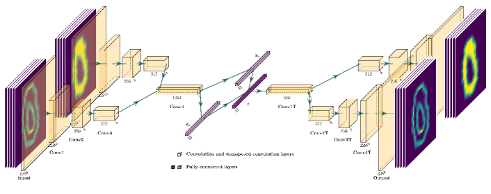
Figure 1: Architecture of our proposed multi-branch VAE

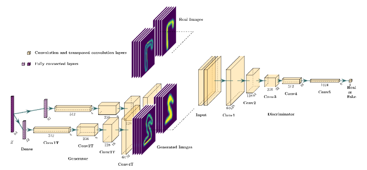
Figure 2: Architecture of multi-branch GAN

II-C Reconstruction Algorithm

Solving (3) using the synergistic regularizer $R_{\mathrm{syn}}=R_{\bm{\theta}}$ defined in (5) is achieved by alternating minimization in $\{\bm{z}_{p}\}$ and $\{\bm{x}_{k}\}$. Given a current estimate $\bm{x}_{k}^{(q)}$ at iteration $q$, the new estimate at iteration $q+1$ is given by

$$\bm{z}_{p}^{(q)}={} \operatornamewithlimits{arg\,min}_{\bm{z}\in\mathcal{Z}}\,\sum_{k=1}^{K}\frac{\eta_{k}}{2}\left\|\bm{G}^{k}_{\bm{\theta}}(\bm{z})-\bm{P}_{p}\bm{x}_{k}^{(q)}\right\|_{2}^{2}+\alpha H(\bm{z})$$

$$\quad\forall p=1,\dots,P$$ (10)

$$\bm{x}_{k}^{(q+1)}={} \operatornamewithlimits{arg\,min}_{\bm{x}\in\mathcal{X}}\,L_{k}(\bm{y}_{k},\bar{\bm{y}}_{k}(\bm{x}))$$

$$+\frac{\beta}{2}\sum_{p=1}^{P}\left\|\bm{G}^{k}_{\bm{\theta}}\left(\bm{z}_{p}^{(q)}\right)-\bm{P}_{p}\bm{x}\right\|^{2}_{2}\quad\forall k=1,\dots,K$$ (11)

Both sub-minimizations can be achieved with iterative algorithms initialized from the previous estimates $\bm{z}_{p}^{(q)}$ and $\bm{x}_{k}^{(q)}$. The $\bm{x}$-update (11) depends on the loss $L_{k}$ and the forward model $\bar{\bm{y}}_{k}$. Note that it is possible to use different $\beta$-values for each $k$ in (11) to adjust the strength of $R_{\bm{\theta}}$ for each channel.

We implemented the $\bm{z}$-update step (10) with a LBFGS algorithm [43] for VAE. However, we observed that LBFGS performed poorly with GAN due to the sensitivity to the initialization in the latent space.

To get around this problem, we used a metaheuristic algorithm that relies on candidate solutions in a defined search space called PSO [44]. The algorithm does not rely on the gradient of the objective being optimized which means the problem does not have to be differentiable [45]. In our study, we used a Python implementation of the variant quantum-behaved PSO [44].

III Results

In this section, we show some results of our methodology for $K=2$. For simplicity, and to solely focus on the inter-channel dependencies, we used $H\equiv 0$, i.e., no regularization on $\bm{z}$. Our generative model-based regularizer is

$$R_{\bm{\theta}}(\bm{x}_{1},\bm{x}_{2})=\min_{\{\bm{z}_{p}\}\in\mathcal{Z}^{P}}\,\Bigg{(}\sum_{p=1}^{P}\frac{\eta}{2}\left\|\bm{\mathcal{G}}^{1}_{\bm{\theta}}(\bm{z}_{p})-\bm{P}_{p}\bm{x}_{1}\right\|^{2}+\frac{1-\eta}{2}\left\|\bm{\mathcal{G}}^{2}_{\bm{\theta}}(\bm{z}_{p})-\bm{P}_{p}\bm{x}_{1}\right\|^{2}\Bigg{)}$$ (12)

where $\eta\in[0,1]$. The reconstructed images are defined as

$$(\hat{\bm{x}}_{1}^{\eta},\hat{\bm{x}}_{2}^{\eta})\triangleq\operatornamewithlimits{arg\,min}_{\bm{x}_{1},\bm{x}_{2}}\,\eta L_{1}(\bm{y}_{1},\bar{\bm{y}}_{1}(\bm{x}_{1}))+(1-\eta)L_{2}(\bm{y}_{2},\bar{\bm{y}}_{2}(\bm{x}_{2}))+\beta R_{\bm{\theta}}(\bm{x}_{1},\bm{x}_{2})\,.$$ (13)

The quality of the reconstructed images $(\hat{\bm{x}}_{1}^{\eta},\hat{\bm{x}}_{2}^{\eta})$ was assessed using the PSNR with respect to the GT images $(\bm{x}_{1}^{\star},\bm{x}_{2}^{\star})$. The function peak_signal_noise_ratio from the Python package skimage.metrics was used to compute the PSNR. The training of the architectures was implemented on a single Nvidia RTX A6000 GPU.

Section III-A presents an evaluation based on the MNIST dataset [31] (reshaped to 32$\times$32), while Section III-B presents results of our multi-branch VAE model for PET/CT joint reconstruction from synthetic projection data generated from real patient images.

III-A MNIST Data

III-A1 Data and Training

The database consists of a collection of 70,000 32$\times$32 image pairs representing digits from 0 to 9 with various shapes (see Figure LABEL:subfig:x1_mnist). These images play the role of the first channel, i.e., $\bm{x}_{1}$. The second channel images $\bm{x}_{2}$ are derived from $\bm{x}_{1}$ using a Roberts Edge filter from scikit-image [46] followed by a Gaussian filter. Figure 3 shows an example of training image pairs.

For this experiment the images coincide with the patches, that is to say, $P=1$, $d=m=1024$, and $\bm{P}_{1}=\mathrm{id}_{\mathcal{X}}$ (identity operator on $\mathcal{X}$).

(a)

(b)

Figure 3: Example of $\bm{x}_{1},\bm{x}_{2}$ image pairs derived from the MNIST dataset used to train the 2 models.

Both VAE and GAN models were trained in an unsupervised manner using 60,000 image pairs for training and 10,000 image pairs for validation. All models were trained using the Adam optimizer with a learning rate of $10^{-4}$. The batch size was chosen experimentally to balance between memory and time constraints. For the VAE training occurs in batches of 10,240 for 10,000 epochs. While the multi-branch GAN model was done in batches of 16,384 for 1,000 epochs.

III-A2 Results

Image Generation

Figures 4 and 5 show generated images using respectively the VAE model and GAN model, using a random $\bm{z}$ generated by uniformity sampling each of its coordinates on $[-3,3]$. The images are distorted digits, similar to the training dataset. We observe that images generated from the same $\bm{z}$ correspond to each other, which suggests that both generators were able to learn from the pairs as opposed to each image individually. We also observed that the GAN-generated images are somehow sharper than the VAE-generated ones.

(a)

(b)

Figure 4: VAE-generated image pairs $(\bm{\mathcal{G}}^{1}_{\bm{\theta}}(\bm{z}),\bm{\mathcal{G}}^{2}_{\bm{\theta}}(\bm{z}))$, using the MNIST-trained models, with random $\bm{z}\in\mathcal{Z}$. The sub-images on LABEL:subfig:vae_1 and LABEL:subfig:vae_2 at same position were generated from the same $\bm{z}$

(a)

(b)

Figure 5: GAN-generated image pairs $(\bm{\mathcal{G}}^{1}_{\bm{\theta}}(\bm{z}),\bm{\mathcal{G}}^{2}_{\bm{\theta}}(\bm{z}))$ with random $\bm{z}\in\mathcal{Z}$. The sub-images on LABEL:subfig:gan_1 and LABEL:subfig:gan_2 at same position were generated from the same $\bm{z}$

Image Prediction: $\bm{x}_{1}$ to $\bm{x}_{2}$ and $\bm{x}_{2}$ to $\bm{x}_{1}$

We define the “model-fitting” function $f_{\eta}$, which evaluates the goodness of the fit between two target images $\bm{x}^{\star}_{1},\bm{x}^{\star}_{2}$ and the generated pair from a trained two-channel model $\bm{\mathcal{G}}^{1}_{\bm{\theta}}(\bm{z}),\bm{\mathcal{G}}^{2}_{\bm{\theta}}(\bm{z})$ as

$$f_{\eta}(\bm{z},\bm{x}_{1}^{\star},\bm{x}_{2}^{\star})\triangleq\eta\left\|\bm{\mathcal{G}}^{1}_{\bm{\theta}}(\bm{z})-\bm{x}^{\star}_{1}\right\|_{2}^{2}+(1-\eta)\left\|\bm{\mathcal{G}}^{2}_{\bm{\theta}}(\bm{z})-\bm{x}^{\star}_{2}\right\|_{2}^{2}$$ (14)

The optimal latent variable, denoted $\check{\bm{z}}_{\eta}(\bm{u}_{1},\bm{u}_{2})$ is defined as

$$\check{\bm{z}}_{\eta}(\bm{x}_{1},\bm{x}_{2})\triangleq\operatornamewithlimits{arg\,min}_{\bm{z}\in\mathcal{Z}}f_{\eta}(\bm{z},\bm{x}_{1},\bm{x}_{2})\,,$$ (15)

where we dropped the $(\bm{x}_{1},\bm{x}_{2})$-dependency on the left-hand side to lighten the notation. Finally, the “predicted images” are given by

$$\check{\bm{x}}_{k}^{\eta}=\bm{\mathcal{G}}^{k}_{\bm{\theta}}(\check{\bm{z}}_{\eta}(\bm{x}_{1},\bm{x}_{2}))\,,\quad k=1,2\,.$$ (16)

Thus, $(\check{\bm{x}}_{k}^{\eta},\check{\bm{x}}_{k}^{\eta})$ represents the “best copy” of $(\bm{x}^{\star}_{1},\bm{x}^{\star}_{2})$ where $\eta$ is a weight that dictates which target image the generative model should prioritize. In particular, if $\eta=0$ then the model-fitting process (15) is oblivious to $\bm{x}_{1}$, so that $\hat{\bm{x}}_{1}^{0}$ is a “prediction” of $\bm{x}_{1}^{\star}$ from $\bm{x}_{2}^{\star}$ from the model (and conversely with $\eta=1$).

Figure 6 shows VAE-generated images $(\check{\bm{x}}_{1}^{\eta},\check{\bm{x}}_{2}^{\eta})$ obtained using model-fitting to a target MNIST digit pair $(\bm{x}_{1}^{\star},\bm{x}_{2}^{\star})$ (from the testing) for different values of $\eta$. When $\eta=0.5$, both generated images $(\check{\bm{x}}_{1}^{0.5},\check{\bm{x}}_{2}^{0.5})$ correspond to the targets with almost no visible mismatch. When $\eta=1$, $\check{\bm{x}}_{1}^{1}$ is very similar to $\bm{x}_{1}^{\star}$ as expected, while $\check{\bm{x}}_{2}^{1}$ is somehow similar to $\bm{x}_{2}^{\star}$ (with some distortions), which shows that the model managed to predict an image fairly similar to $\bm{x}_{2}^{\star}$ using $\bm{x}_{1}^{\star}$ only. The converse result is observed with $\eta=0$. This shows that our model has learned images pairwise and has the potential to predict an image from the other.

Figure 6 shows the same results with our GAN model. The generated images are somehow similar to the targets for $\eta=0.5$ and the images are sharper than the VAE-generated image. However, the model seems to have some difficulties with prediction as artifacts are visible on both images for $\eta=0,1$. Additionally, the best results for both images seem to be obtained for $\eta=0.5$, which suggests that the model needs to see both targets for accurate model fitting.

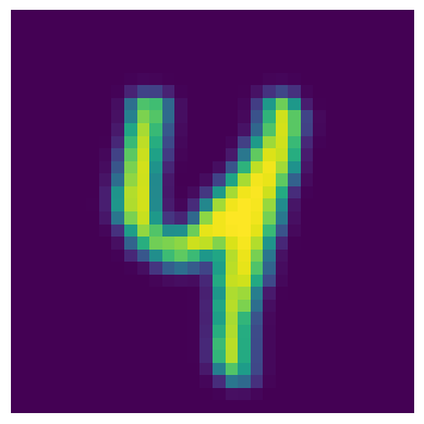
(a)

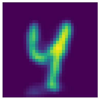
(b)

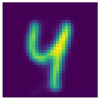
(c)

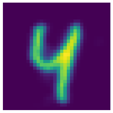
(d)

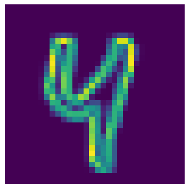
(e)

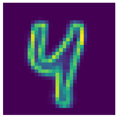
(f)

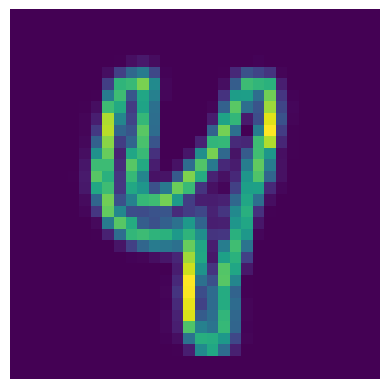
(g)

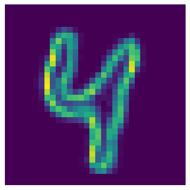
(h)

Figure 6: VAE-generated images $(\check{\bm{x}}_{1}^{\eta},\check{\bm{x}}_{2}^{\eta})$ obtained by model-fitting to a target MNIST digit pair $\bm{x}_{1}^{\star},\bm{x}_{2}^{\star}$ for different values of $\eta$.

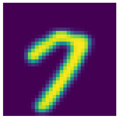
(a)

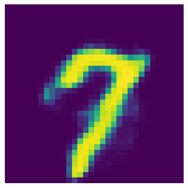
(b)

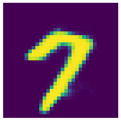
(c)

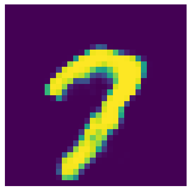
(d)

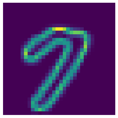
(e)

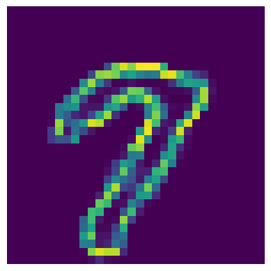
(f)

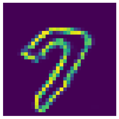
(g)

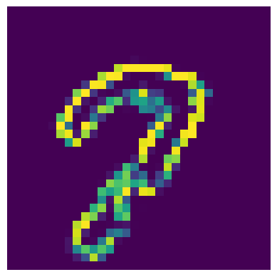
(h)

Figure 7: GAN-generated images $(\check{\bm{x}}_{1}^{\eta},\check{\bm{x}}_{2}^{\eta})$ obtained by model-fitting to a target MNIST digit pair $\bm{x}_{1}^{\star},\bm{x}_{2}^{\star}$ for different values of $\eta$.

Image Denoising

In this section, we focus on denoising two images $\bm{x}_{1}^{\mathrm{n}}$ and $\bm{x}_{2}^{\mathrm{n}}$,

$$\bm{x}^{\mathrm{n}}_{k}=\bm{x}^{\star}_{k}+\bm{\epsilon}_{k}\,,\quad k=1,2$$

where $(\bm{x}_{1}^{\star},\bm{x}_{1}^{\star})$ is a GT image pair (from the testing dataset) and $\epsilon_{k}\sim\mathcal{N}(\bm{0}_{m},\sigma_{k}^{2}\bm{I}_{m})$, using a PLS approach, i.e., solving (3) with $\bm{y}_{k}=\bm{x}^{\mathrm{n}}_{k}$, $\bar{\bm{y}}_{k}=\mathrm{id}_{\mathcal{X}}$, $L_{k}(\bm{y}_{k},\bar{\bm{y}}_{k})=\frac{1}{2}\|\bm{y}_{k}-\bar{\bm{y}}_{k}\|_{2}^{2}$ and using the trained regularizer $R_{\mathrm{syn}}=R_{\bm{\theta}}$ defined in (12). As $P=1$, the image update (11) simplifies to $\bm{x}_{k}^{(q+1)}=\left(\bm{x}^{\mathrm{n}}_{k}+\beta\bm{\mathcal{G}}^{k}_{\bm{\theta}}\left(\bm{z}^{(q+1)}\right)\right)/(1+\beta)$, $k=1,2$ . We used $\beta=1$ for both VAE and GAN. We use $\sigma_{2}>\sigma_{1}$ and $\sigma_{1}>\sigma_{2}$ respectively for the VAE and the GAN model. The denoised images are denoted $\hat{\bm{x}}_{1}^{\eta}$ and $\hat{\bm{x}}_{2}^{\eta}$. Figure 8 (VAE) and Figure 10 (GAN) shows the original noisy images $\bm{x}^{\mathrm{n}}_{k}$ and the denoised images $\hat{\bm{x}}_{k}^{\eta}$. We start by commenting on the VAE results.

For $\eta=0$, the model ignores the first channel and focuses on the second channel only, which is the noisiest. Therefore the model fails to generate the second image, which results in a poor prediction for the first image. The quality of $\hat{\bm{x}}_{1}^{\eta}$ seems to increase as $\eta$ approaches 0.9 (with a slight decrease at $\eta=1$). In contrast, the quality of $\hat{\bm{x}}_{2}^{\eta}$ seems to increase between $\eta=0$ and $0.5$ then slowly decrease from $0.5$ and $1$. These observations are confirmed by the PSNR-$\eta$ curves (Figure 9). This experiment suggests that the less noisy channel does not benefit from the more noisy one while the noisy one benefits from both (best results obtained with $\eta=0.5$)

The results are somehow reversed with the GAN model (Figure 10 and Figure 11), but we observe that the best results are obtained for $\eta=0.5$ for both channels (with a slightly higher PSNR at $\eta=0.1$ for $k=2$). We also observe that the PSNR-$\eta$ curves appear “unstable”. This phenomenon can be attributed to the issues reported with model-fitting for GAN [30].

In conclusion of this experiment, we observe our model performs the best when it denoises the two images simultaneously, suggesting that the multi-branched regularizer manages to convey information from between the two channels.

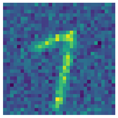
(a)

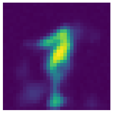
(b)

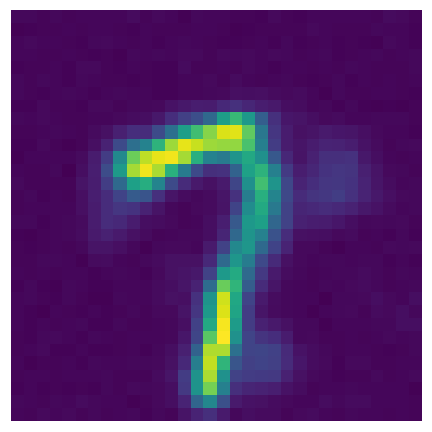
(c)

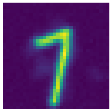
(d)

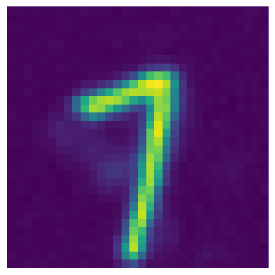
(e)

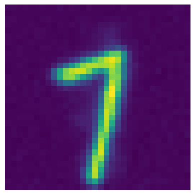
(f)

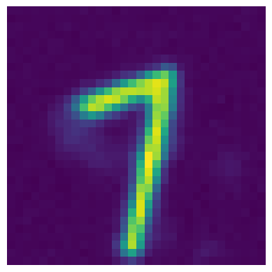
(g)

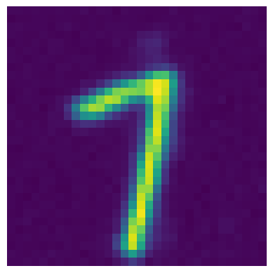
(h)

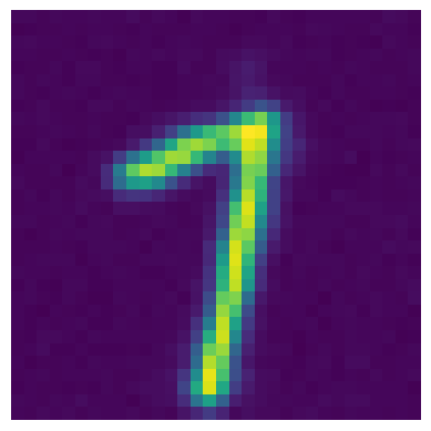
(i)

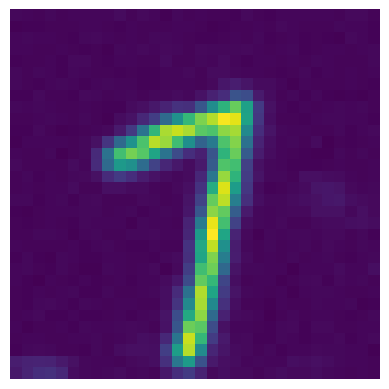
(j)

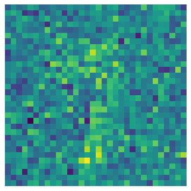
(k)

(l)

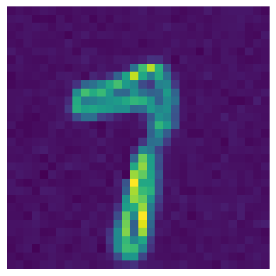
(m)

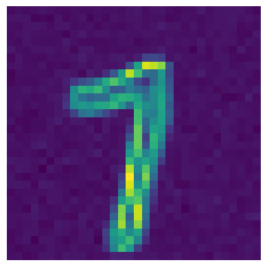
(n)

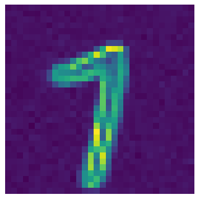
(o)

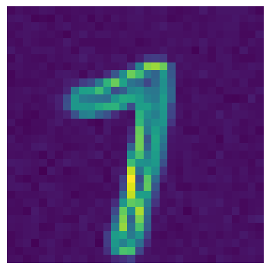
(p)

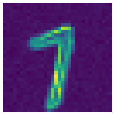
(q)

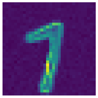
(r)

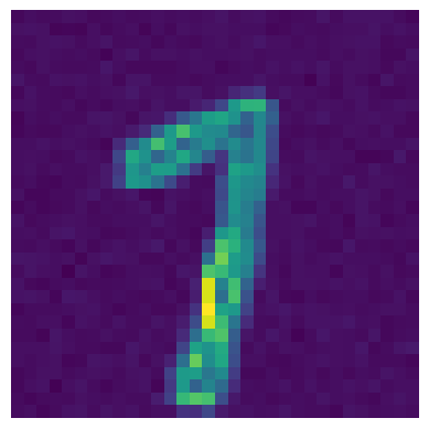
(s)

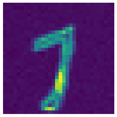
(t)

Figure 8: Noisy $(\bm{x}_{1}^{\mathrm{n}},\bm{x}_{2}^{\mathrm{n}})$ and VAE-denoised images $(\check{\bm{x}}_{1}^{\eta},\check{\bm{x}}_{2}^{\eta})$ for different values of $\eta$.

Figure 9: PSNR values of denoised MNIST images using VAE with respect to $\eta$.

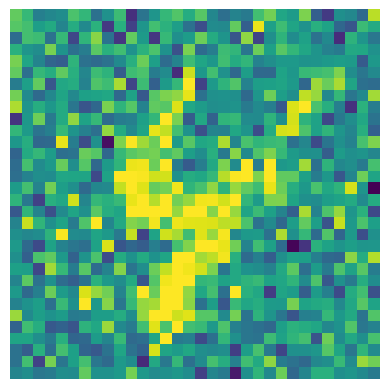
(a)

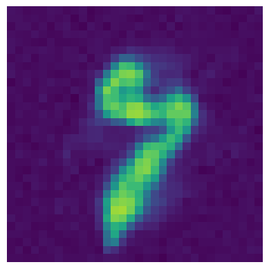
(b)

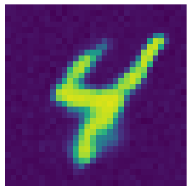
(c)

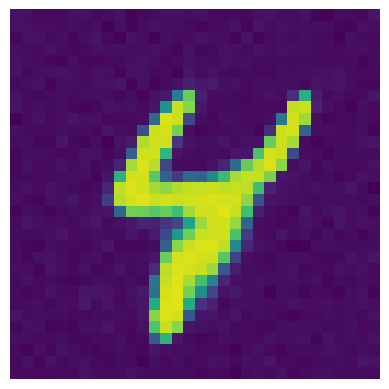
(d)

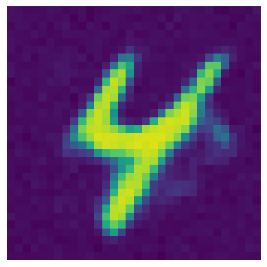
(e)

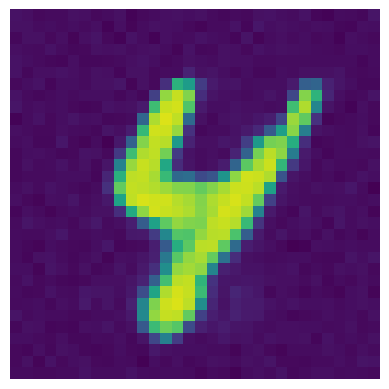
(f)

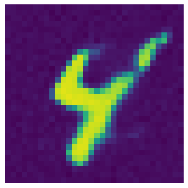
(g)

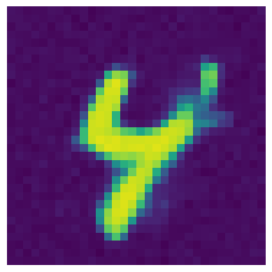
(h)

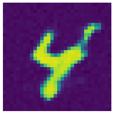
(i)

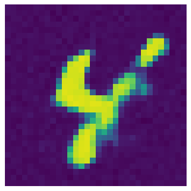
(j)

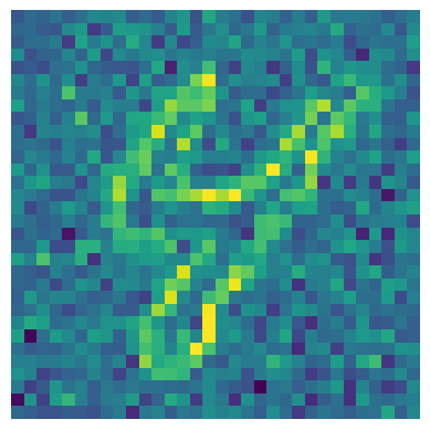
(k)

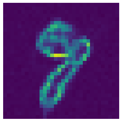
(l)

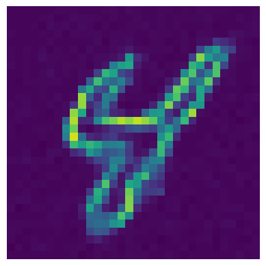
(m)

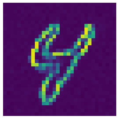
(n)

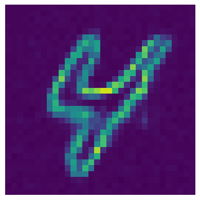
(o)

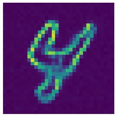
(p)

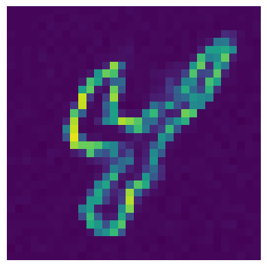
(q)

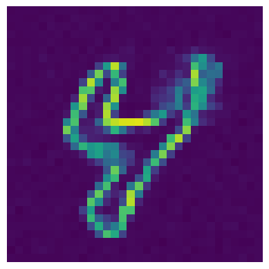
(r)

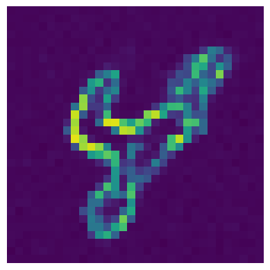
(s)

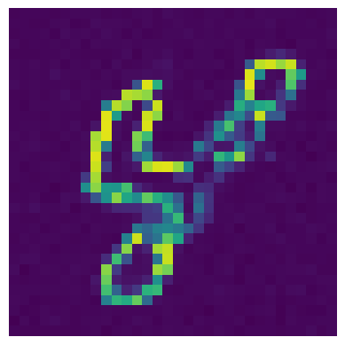
(t)

Figure 10: Noisy images $(\bm{x}_{1}^{\mathrm{n}},\bm{x}_{2}^{\mathrm{n}})$ and GAN-denoised images $(\check{\bm{x}}_{1}^{\eta},\check{\bm{x}}_{2}^{\eta})$ for different values of $\eta$.

Figure 11: PSNR values of denoised MNIST images using GAN with respect to $\eta$.

III-B Synergistic PET/CT Reconstruction

In the following, we only consider the VAE-based regularizer.

III-B1 Data and Training

A collection of 368 abdomens PET/CT image volumes were acquired by Siemens Biograph mCT PET/CT scanner at Centre Hospitalier Universitaire Poitier. Each volume comprises a set of 512$\times$512 slices (0.97 mm pixel size), for a total of 41,000 slices per modality. A $(\bm{x}_{1},\bm{x}_{2})$ pair correspond PET/CT slice pair ($\bm{x}_{1}$ for PET, $\bm{x}_{2}$ for CT). A total of 318 pairs were used for training while 50 pairs were used for testing—testing images and training images came from different patients. $64\times 64$ patches were extracted from each image (with a 75% overlap along each axis, for a total of 2,000 patches pair $(\bm{u}_{1},\bm{u}_{2})$, see Figure 12) then were used to train the VAE model $\bm{\mathcal{G}}_{\bm{\theta}}$ and to define $R_{\bm{\theta}}$ (12). The PET and CT were normalized before training, and the two normalizing constants were incorporated in $R_{\bm{\theta}}$ (12). The Adam optimizer was used for training with a learning rate of 10^-4 and batch size of 4,096 for 1,000 epochs.

(a)

(b)

Figure 12: Examples for PET/CT patch pairs, i.e., $\bm{u}_{1},\bm{u}_{2}$ in (8), used to train our model.

A PET/CT image pair $(\bm{x}_{1}^{\star},\bm{x}_{1}^{\star})$ (Figure 13) was used as a GT. The PET data $\bm{y}_{1}\in\mathbb{R}^{n_{1}}$ and CT data $\bm{y}_{2}\in\mathbb{R}^{n_{2}}$ were generated as

$$\bm{y}_{k}\sim\mathrm{Poisson}\left(\bar{\bm{y}}_{k}\left(\bm{x}_{k}^{\star}\right)\right),\quad k=1,2$$ (17)

where $\bar{\bm{y}}_{1}\colon\mathbb{R}^{m}\to\mathbb{R}^{n_{1}}$ and $\bar{\bm{y}}_{2}\colon\mathbb{R}^{m}\to\mathbb{R}^{n_{2}}$ are respectively the PET and CT forward model, and $n_{1}$ and $n_{2}$ are respectively the number of PET LoR and the number of CT beams.

(a)

(b)

Figure 13: PET and CT GT images $\bm{x}_{1}^{\star}$ and $\bm{x}_{2}^{\star}$.

The PET forward model is

$$\bar{\bm{y}}_{1}(\bm{x}_{1})=\tau\bm{P}\bm{x}\,,\quad\forall\bm{x}_{1}\in\mathcal{X}$$ (18)

where $\bm{P}\in\mathbb{R}^{{n_{1}}\times m}$ is the PET system matrix that incorporates the 511 keV attenuation coefficients, $\bm{x}_{1}$ is the radiotracer distribution and $\tau$ is the acquisition time. The PET attenuation factors were obtained by converting $\bm{x}^{\star}_{2}$ to a 511-keV attenuation image using the method proposed in [47]. We used a homemade parallel-beam projector for $\bm{P}$ with 120 angles of view from 0^∘ to 360^∘ and 512 beams.

The (monochromatic) CT forward model we used is

$$\bar{\bm{y}}_{2}(\bm{x}_{2})=I\cdot\exp(-\bm{A}\bm{x}_{2})\,,\quad\forall\bm{x}\in\mathcal{X},$$ (19)

where $I$ is X-ray intensity, $\bm{A}\in\mathbb{R}^{n_{2}\times m}$ is the CT system matrix (fan-beam transform), $\bm{x}_{2}$ is the attenuation image, and the $\exp$ function applied to a vector should be understood as operating on each element individually. Both PET and CT acquisitions were tuned to simulate low-count imaging by tuning $\tau$ in (18) and $I$ in (19). We implemented the projection matrix $\bm{A}$ using ASTRA [48] as a fan-beam projector with a source-to-origin distance of 600 mm and an origin-to-detector distance of 600 mm, utilizing 750 detectors with a width of 1.2 mm each and capturing 120 angles of view from 0^∘ to 360^∘.

III-B2 Results

Image Generation

Figure 14 shows images of generated images patches using respectively the VAE PET/CT model, using a random $\bm{z}$ generated similarly as for the MNIST model in Section III-A2. The images generated from the PET model $\bm{\mathcal{G}}^{1}_{\bm{\theta}}$ (Figure LABEL:subfig:vae_lungs_pet64) appear blurry while those generated from the CT model $\bm{\mathcal{G}}^{2}_{\bm{\theta}}$ (Figure LABEL:subfig:vae_lungs_ct64) are sharper. Some structural similarities can be observed (cf. the magnified areas in Figure 14), which suggests that information is shared between the two modalities. However, these similarities are less pronounced than the MNIST-trained model.

(a)

(b)

Figure 14: VAE-generated image pairs $(\bm{\mathcal{G}}^{1}_{\bm{\theta}}(\bm{z}),\bm{\mathcal{G}}^{2}_{\bm{\theta}}(\bm{z}))$ with random $\bm{z}\in\mathcal{Z}$, using the PET/CT-trained models, with random $\bm{z}\in\mathcal{Z}$. The sub-images on LABEL:subfig:vae_1 and LABEL:subfig:vae_2 at same position were generated from the same $\bm{z}$

Image Reconstruction

Joint reconstruction of $(\bm{x}_{1},\bm{x}_{2})$ is achieved by solving (3) with $L_{k}(\bm{y}_{k},\bar{\bm{y}}_{k})=\sum_{i=1}^{n_{k}}-y_{i,k}\log\bar{y}_{i,k}+\bar{y}_{i,k}$ (negative Poisson log-likelihood with the convention $0\cdot\log 0=0$), the trained regularizer $R_{\mathrm{syn}}=R_{\bm{\theta}}$, and using the algorithm iteratively defined by (10) and (11). The patch extractors $\bm{P}_{p}$ were the same as those used in training (75% overlap along each axis).

We used a modified EM algorithm [49] for the $\bm{x}_{1}$-update with 50 iterations. For the $\bm{x}_{2}$-update, we performed a WLS reconstruction using a SPS algorithm [12] with 150 iterations. The attenuation correction factors were obtained from a scout reconstruction of the attenuation image $\bm{x}_{2}$ from $\bm{y}_{2}$ using an unregularized WLS reconstruction, then converted into 511-keV images using the method proposed by [47] [47]. We used the LBFGS algorithm for $\bm{z}$-fitting with maximum iteration set at 200 for the VAE model. Both reconstructions were compared with standard EM (for PET) and WLS (for CT).

The scanner data $\bm{y}_{1}$ and $\bm{y}_{2}$ were acquired following (17) with 2 settings: (i) $\tau=300$ and $I=700$ (high-count PET, low-count CT), and (ii) $\tau=10$ and $I=4.5\cot 10^{4}$ (low-count PET, high-count CT). We used two different $\beta$-values for the PET and the CT. The $\beta$-values were adjusted so that the contribution of $R_{\bm{\theta}}$ is the same in both settings. We present the results in the two following paragraphs.

High-count PET, low-count CT

Reconstructed images $\hat{\bm{x}}_{1}^{\eta}$ and $\hat{\bm{x}}_{2}^{\eta}$ for $\eta$ ranging from $0$ to $1$ are shown in Figures 15, alongside the EM-reconstructed PET image $\hat{\bm{x}}_{1}^{\mathrm{em}}$ (Figure LABEL:subfig:mlem_pet64) and the WLS-reconstructed CT image $\hat{\bm{x}}_{2}^{\mathrm{wls}}$ (Figure LABEL:subfig:wls_ct64). The PSNR values are also displayed for each image. Both EM-PET and WLS-PET images appear noisy as expected as their reconstructions were not regularized (especially the WLS-PET). The optimal PET reconstruction is obtained with our model with $\eta=0.75$, while the optimal CT image is obtained with $\eta=0.5$. This suggests that both modalities benefit from each other, although the CT can be further improved with a greater contribution from the CT. However, the CT images appear blurry as the ribs and the spine are barely visible. Blurry images are a well-known problem with VAE which was reported in [30].

\begin{overpic}[width=65.04034pt]{images/vae/lungs/pet/patch64/full_recon/fullpet_halfct/sc700i300bp14k/eta0.5/pet_mlem_psnr31.36_ssim0.9874.png} \put(1.0,4.0){ {\color[rgb]{1,0,0}\small PSNR=31.36} } \end{overpic}

(a)

\begin{overpic}[width=65.04034pt]{images/vae/lungs/pet/patch64/full_recon/fullpet_halfct/sc700i300bp14k/eta0.01/pet_recon_iter9_psnr29.87_ssim0.9917.png} \put(1.0,4.0){ {\color[rgb]{1,0,0}\small PSNR=29.87} } \par\end{overpic}

(b)

\begin{overpic}[width=65.04034pt]{images/vae/lungs/pet/patch64/full_recon/fullpet_halfct/sc700i300bp14k/eta0.25/pet_recon_iter9_psnr35.93_ssim0.9958.png} \put(1.0,4.0){ {\color[rgb]{1,0,0}\small PSNR=35.93} } \end{overpic}

(c)

\begin{overpic}[width=65.04034pt]{images/vae/lungs/pet/patch64/full_recon/fullpet_halfct/sc700i300bp14k/eta0.5/pet_recon_iter9_psnr36.57_ssim0.9963.png} \put(1.0,4.0){ {\color[rgb]{1,0,0}\small PSNR=36.57} } \end{overpic}

(d)

\begin{overpic}[width=65.04034pt]{images/vae/lungs/pet/patch64/full_recon/fullpet_halfct/sc700i300bp14k/eta0.75/pet_recon_iter9_psnr37.65_ssim0.9967.png} \put(1.0,4.0){ {\color[rgb]{1,0,0}\small PSNR=37.65} } \end{overpic}

(e)

\begin{overpic}[width=65.04034pt]{images/vae/lungs/pet/patch64/full_recon/fullpet_halfct/sc700i300bp14k/eta0.99/pet_recon_iter9_psnr35.52_ssim0.9969.png} \put(1.0,4.0){ {\color[rgb]{1,0,0}\small PSNR=35.52} } \end{overpic}

(f)

\begin{overpic}[width=65.04034pt]{images/vae/lungs/ct/patch64/full_recon/eta0.5/sc700i300/ct_wls_psnr19.54_ssim0.9992.png} \put(1.0,4.0){ {\color[rgb]{1,0,0}\small PSNR=19.54} } \end{overpic}

(g)

\begin{overpic}[width=65.04034pt]{images/vae/lungs/ct/patch64/full_recon/eta0.01/sc700i300/ct_recon_iter9_psnr28.53_ssim0.9998.png} \put(1.0,4.0){ {\color[rgb]{1,0,0}\small PSNR=28.53} } \end{overpic}

(h)

\begin{overpic}[width=65.04034pt]{images/vae/lungs/ct/patch64/full_recon/eta0.25/sc700i300/ct_recon_iter9_psnr28.68_ssim0.9998.png} \put(1.0,4.0){ {\color[rgb]{1,0,0}\small PSNR=28.68} } \end{overpic}

(i)

\begin{overpic}[width=65.04034pt]{images/vae/lungs/ct/patch64/full_recon/eta0.5/sc700i300/ct_recon_iter9_psnr28.49_ssim0.9998.png} \put(1.0,4.0){ {\color[rgb]{1,0,0}\small PSNR=28.49} } \end{overpic}

(j)

\begin{overpic}[width=65.04034pt]{images/vae/lungs/ct/patch64/full_recon/eta0.75/sc700i300/ct_recon_iter9_psnr28.50_ssim0.9998.png} \put(1.0,4.0){ {\color[rgb]{1,0,0}\small PSNR=28.50} } \end{overpic}

(k)

\begin{overpic}[width=65.04034pt]{images/vae/lungs/ct/patch64/full_recon/eta0.99/sc700i300/ct_recon_iter9_psnr27.66_ssim0.9997.png} \put(1.0,4.0){ {\color[rgb]{1,0,0}\small PSNR=27.66} } \end{overpic}

(l)

Figure 15: PET and CT reconstructions using the proposed methods with high-count PET, low-count CT.

Low-count PET, high-count CT

Reconstructed images in Figures 16. The best CT reconstruction is obtained by the WLS reconstruction, which is expected as we used high-count projection data. The PSNR of the reconstructed images decreases. On the other hand, the best PET reconstruction in terms of PSNR is obtained with $\eta=0.75$, as the CT information prevents the model from overfitting with the noise in the PET data. The PSNR drops with $\eta=0.99$, when the CT information vanishes. This result highlights the contribution from the CT to the PET.

\begin{overpic}[width=65.04034pt]{images/vae/lungs/pet/patch64/full_recon/halfpet_fullct/sc20i3000bp200/eta0.5/pet_mlem_psnr20.22_ssim0.9102.png} \put(1.0,4.0){ {\color[rgb]{1,0,0}\small PSNR=20.22} } \end{overpic}

(a)

\begin{overpic}[width=65.04034pt]{images/vae/lungs/pet/patch64/full_recon/halfpet_fullct/sc20i3000bp200/eta0.01/pet_recon_iter9_psnr30.10_ssim0.9904.png} \put(1.0,4.0){ {\color[rgb]{1,0,0}\small PSNR=30.10} } \end{overpic}

(b)

\begin{overpic}[width=65.04034pt]{images/vae/lungs/pet/patch64/full_recon/halfpet_fullct/sc20i3000bp200/eta0.25/pet_recon_iter9_psnr34.68_ssim0.9936} \put(1.0,4.0){ {\color[rgb]{1,0,0}\small PSNR=34.68} } \end{overpic}

(c)

\begin{overpic}[width=65.04034pt]{images/vae/lungs/pet/patch64/full_recon/halfpet_fullct/sc20i3000bp200/eta0.5/pet_recon_iter9_psnr34.81_ssim0.9938.png} \put(1.0,4.0){ {\color[rgb]{1,0,0}\small PSNR=34.81} } \end{overpic}

(d)

\begin{overpic}[width=65.04034pt]{images/vae/lungs/pet/patch64/full_recon/halfpet_fullct/sc20i3000bp200/eta0.75/pet_recon_iter9_psnr35.28_ssim0.9939.png} \put(1.0,4.0){ {\color[rgb]{1,0,0}\small PSNR=35.28} } \end{overpic}

(e)

\begin{overpic}[width=65.04034pt]{images/vae/lungs/pet/patch64/full_recon/halfpet_fullct/sc20i3000bp200/eta0.99/pet_recon_iter9_psnr34.41_ssim0.9931.png} \put(1.0,4.0){ {\color[rgb]{1,0,0}\small PSNR=34.41} } \end{overpic}

(f)

\begin{overpic}[width=65.04034pt]{images/vae/lungs/ct/patch64/full_recon/halfpet_fullct/sc20i3000v2/eta0.5/ct_wls_psnr30.47_ssim0.9999.png} \put(1.0,4.0){ {\color[rgb]{1,0,0}\small PSNR=30.47} } \end{overpic}

(g)

\begin{overpic}[width=65.04034pt]{images/vae/lungs/ct/patch64/full_recon/halfpet_fullct/sc20i3000v2/eta0.01/ct_recon_iter3_psnr29.74_ssim0.9999.png} \put(1.0,4.0){ {\color[rgb]{1,0,0}\small PSNR=29.74} } \end{overpic}

(h)

\begin{overpic}[width=65.04034pt]{images/vae/lungs/ct/patch64/full_recon/halfpet_fullct/sc20i3000v2/eta0.25/ct_recon_iter3_psnr29.70_ssim0.9999.png} \put(1.0,4.0){ {\color[rgb]{1,0,0}\small PSNR=29.70} } \end{overpic}

(i)

\begin{overpic}[width=65.04034pt]{images/vae/lungs/ct/patch64/full_recon/halfpet_fullct/sc20i3000v2/eta0.5/ct_recon_iter3_psnr29.64_ssim0.9999.png} \put(1.0,4.0){ {\color[rgb]{1,0,0}\small PSNR=29.64} } \end{overpic}

(j)

\begin{overpic}[width=65.04034pt]{images/vae/lungs/ct/patch64/full_recon/halfpet_fullct/sc20i3000v2/eta0.75/ct_recon_iter3_psnr29.65_ssim0.9999.png} \put(1.0,4.0){ {\color[rgb]{1,0,0}\small PSNR=29.65} } \end{overpic}

(k)

\begin{overpic}[width=65.04034pt]{images/vae/lungs/ct/patch64/full_recon/halfpet_fullct/sc20i3000v2/eta0.99/ct_recon_iter3_psnr27.85_ssim0.9998.png} \put(1.0,4.0){ {\color[rgb]{1,0,0}\small PSNR=27.85} } \end{overpic}

(l)

Figure 16: PET and CT reconstructions using the proposed methods with low-count PET, high-count CT.

IV Discussion

This work follows up on our previous studies presented in [28, 29], where we initially trained our models on full images. However, we encountered potential overfitting issues due to the lack of data for training, resulting in overly optimistic results. To address this challenge, we adopted a patch decomposition approach. It has been previously reported that training on repetitive and consistent patches yields better results than training on the entire image [39]. To mitigate artifacts in the reconstructed images, our regularization strategy necessitates numerous overlapping patches. However, this comes at the expense of increased computational cost, as each patch requires its own latent variable.

We demonstrated that our models successfully learn from two images simultaneously, suggesting their applicability in a framework akin to multichannel DiL for image reconstruction. Results obtained with MNIST-trained models distinctly showcase how our generative model-based regularizers effectively utilize information from both images for denoising. Furthermore, the multi-branch architecture of our model did not suffer from cross-modal imprinting as observed in [50]. It also does not prioritize one modality at the expense of the other as observed in [27]. However, this effect is less pronounced in PET/CT images. This limitation can be attributed to the utilization of small patches, which restrict the model’s ability to capture more “global” inter-modal information. While using larger patches could address this issue, it may require more training data and may lead to increased computational burden due to the need for significant patch overlap to prevent artifacts.

We focused on VAE for PET/CT reconstruction due to the observed model-fitting (minimization w.r.t. $\bm{z}$) issues with GAN. However, VAE is known to produce blurry images. While this limitation may be acceptable for PET due to its low intrinsic resolution, it poses challenges for CT and MRI reconstructions.

While we have demonstrated that multi-branch generative models offer a viable approach for learned synergistic reconstruction, it’s important to explore alternative options beyond VAE and GAN. DM have shown significant promise in generating high-quality images from training datasets [51]. These models can be seamlessly integrated into a PML reconstruction framework, as demonstrated by DPS [52]. Recent advancements in spectral CT reconstruction have further highlighted the potential of DM. Studies have shown that DM are capable of capturing multi-channel information and employing multi-channel DPS leads to superior spectral CT images compared to conventional techniques [53, 54]. More specifically, they demonstrated that single-image DPS achieves better results than conventional synergistic reconstruction, and that joint DPS outperforms single-image DPS. Therefore, the future of learned synergistic reconstruction may shift towards leveraging DM.

V Conclusion

In conclusion, our study highlights the utility of generative models for learned synergistic reconstruction in medical imaging. By training on pairs of images, our approach harnesses the power of VAE and GAN to improve denoising and reconstruction outcomes. While challenges such as patch decomposition and inherent model limitations persist, our results demonstrate promising advancements in leveraging generative models for enhancing image quality and information exchange between modalities. Moving forward, further exploration of alternative models, such as DM, may offer additional avenues for enhancing imaging outcomes in medical diagnostics and research. Overall, our findings contribute to the growing body of literature on learned synergistic reconstruction methods and pave the way for future developments in medical multimodal imaging technology.

References

- [1] Luis Gómez-Chova, Devis Tuia, Gabriele Moser and Gustau Camps-Valls “Multimodal Classification of Remote Sensing Images: A Review and Future Directions” In Proceedings of the IEEE 103.9, 2015, pp. 1560–1584 DOI: 10.1109/JPROC.2015.2449668
- [2] M. Dalla Mura, S. Prasad, F. Pacifici, P. Gamba, J. Chanussot and J.. Benediktsson “Challenges and Opportunities of Multimodality and Data Fusion in Remote Sensing” In Proceedings of the IEEE 103.9, 2015, pp. 1585–1601 DOI: 10.1109/JPROC.2015.2462751
- [3] Teng Xue, Weiming Wang, Jin Ma, Wenhai Liu, Zhenyu Pan and Mingshuo Han “Progress and Prospects of Multimodal Fusion Methods in Physical Human–Robot Interaction: A Review” In IEEE Sensors Journal 20.18, 2020, pp. 10355–10370 DOI: 10.1109/JSEN.2020.2995271
- [4] Hang Su, Wen Qi, Jiahao Chen, Chenguang Yang, Juan Sandoval and Med Amine Laribi “Recent advancements in multimodal human–robot interaction” In Frontiers in Neurorobotics 17, 2023, pp. 1084000 DOI: 10.3389/fnbot.2023.1084000
- [5] Bernd J. Pichler, Martin S. Judenhofer and Christina Pfannenberg “Multimodal Imaging Approaches: PET/CT and PET/MRI” In Molecular Imaging I 185/1, Handbook of Experimental Pharmacology Berlin, Heidelberg: Springer Berlin Heidelberg, 2008, pp. 109–132 DOI: 10.1007/978-3-540-72718-7˙6
- [6] Pierre Decazes, Pauline Hinault, Ovidiu Veresezan, Sébastien Thureau, Pierrick Gouel and Pierre Vera “Trimodality PET/CT/MRI and Radiotherapy: A Mini-Review” In Frontiers in Oncology 10, 2021, pp. 614008 DOI: 10.3389/fonc.2020.614008
- [7] Dale L Bailey, Michael N Maisey, David W Townsend and Peter E Valk “Positron emission tomography” Springer, 2005
- [8] Frank Natterer “The mathematics of computerized tomography” SIAM, 2001
- [9] L.. Shepp and Y. Vardi “Maximum Likelihood Reconstruction for Emission Tomography” In IEEE Transactions on Medical Imaging 1.2, 1982, pp. 113–122 DOI: 10.1109/TMI.1982.4307558
- [10] Peter J Green “Bayesian reconstructions from emission tomography data using a modified EM algorithm” In IEEE transactions on medical imaging 9.1 IEEE, 1990, pp. 84–93
- [11] Alvaro R De Pierro “A modified expectation maximization algorithm for penalized likelihood estimation in emission tomography” In IEEE transactions on medical imaging 14.1 IEEE, 1995, pp. 132–137
- [12] I.. Elbakri and J.. Fessler “Statistical image reconstruction for polyenergetic X-ray computed tomography” In IEEE transactions on medical imaging 21.2 IEEE, 2002, pp. 89–99
- [13] Peter Blomgren and Tony F Chan “Color TV: total variation methods for restoration of vector-valued images” In IEEE transactions on image processing 7.3 IEEE, 1998, pp. 304–309
- [14] Abolfazl Mehranian, Martin A Belzunce, Claudia Prieto, Alexander Hammers and Andrew J Reader “Synergistic PET and SENSE MR image reconstruction using joint sparsity regularization” In IEEE transactions on medical imaging 37.1 IEEE, 2017, pp. 20–34
- [15] Matthias J Ehrhardt, Kris Thielemans, Luis Pizarro, David Atkinson, Sébastien Ourselin, Brian F Hutton and Simon R Arridge “Joint reconstruction of PET-MRI by exploiting structural similarity” In Inverse Problems 31.1 IOP Publishing, 2014, pp. 015001
- [16] David S Rigie and Patrick J La Rivière “Joint reconstruction of multi-channel, spectral CT data via constrained total nuclear variation minimization” In Physics in Medicine & Biology 60.5 IOP Publishing, 2015, pp. 1741
- [17] Simon R Arridge, Matthias J Ehrhardt and Kris Thielemans “(An overview of) Synergistic reconstruction for multimodality/multichannel imaging methods” In Philosophical Transactions of the Royal Society A 379.2200 The Royal Society Publishing, 2021, pp. 20200205
- [18] Qiong Xu, Hengyong Yu, Xuanqin Mou, Lei Zhang, Jiang Hsieh and Ge Wang “Low-dose X-ray CT reconstruction via dictionary learning” In IEEE transactions on medical imaging 31.9 IEEE, 2012, pp. 1682–1697
- [19] Yanbo Zhang, Xuanqin Mou, Ge Wang and Hengyong Yu “Tensor-based dictionary learning for spectral CT reconstruction” In IEEE transactions on medical imaging 36.1 IEEE, 2016, pp. 142–154
- [20] Yi Zhang, Yan Xi, Qingsong Yang, Wenxiang Cong, Jiliu Zhou and Ge Wang “Spectral CT reconstruction with image sparsity and spectral mean” In IEEE transactions on computational imaging 2.4 IEEE, 2016, pp. 510–523
- [21] Weiwen Wu, Yanbo Zhang, Qian Wang, Fenglin Liu, Peijun Chen and Hengyong Yu “Low-dose spectral CT reconstruction using image gradient –norm and tensor dictionary” In Applied Mathematical Modelling 63 Elsevier, 2018, pp. 538–557
- [22] Xuru Li, Xueqin Sun, Yanbo Zhang, Jinxiao Pan and Ping Chen “Tensor Dictionary Learning with an Enhanced Sparsity Constraint for Sparse-View Spectral CT Reconstruction” In Photonics 9.1, 2022, pp. 35 MDPI
- [23] Alexandre Bousse, Venkata Sai Sundar Kandarpa, Simon Rit, Alessandro Perelli, Mengzhou Li, Guobao Wang, Jian Zhou and Ge Wang “Systematic Review on Learning-based Spectral CT” In IEEE Transactions on Radiation and Plasma Medical Sciences, 2023 DOI: 10.1109/TRPMS.2023.3314131
- [24] Viswanath P Sudarshan, Gary F Egan, Zhaolin Chen and Suyash P Awate “Joint PET-MRI image reconstruction using a patch-based joint-dictionary prior” In Medical image analysis 62 Elsevier, 2020, pp. 101669
- [25] Alessandro Perelli, Suxer Alfonso Garcia, Alexandre Bousse, Jean-Pierre Tasu, Nikolaos Efthimiadis and Dimitris Visvikis “Multi-channel convolutional analysis operator learning for dual-energy CT reconstruction” In Physics in Medicine & Biology 67.6 IOP Publishing, 2022, pp. 065001
- [26] Guillaume Corda-D’Incan, Julia A Schnabel, Alexander Hammers and Andrew J Reader “Single-modality supervised joint PET-MR image reconstruction” In IEEE Transactions on Radiation and Plasma Medical Sciences IEEE, 2023
- [27] Zhaoheng Xie, Tiantian Li, Xuezhu Zhang, Wenyuan Qi, Evren Asma and Jinyi Qi “Anatomically aided PET image reconstruction using deep neural networks” In Medical Physics 48.9, 2021, pp. 5244–5258
- [28] N.. Pinton, A. Bousse, Z. Wang, C. Cheze-Le-Rest, V. Maxim, C. Comtat, F. Sureau and D. Visvikis “Synergistic PET/CT Reconstruction Using a Joint Generative Model” In International Conference on Fully Three-Dimensional Image Reconstruction in Radiology and Nuclear Medicine, 2023
- [29] N.. Pinton, A Bousse, C. Cheze-Le-Rest and D. Visvikis “Joint PET/CT Reconstruction Using a Double Variational Autoencoder” In IEEE Nuclear Science Symposium Medical Imaging Conference and Room Temperature Semiconductor Conference, 2023
- [30] Margaret Duff, Neill DF Campbell and Matthias J Ehrhardt “Regularising inverse problems with generative machine learning models” In arXiv preprint arXiv:2107.11191, 2021
- [31] Li Deng “The MNIST database of handwritten digit images for machine learning research [best of the web]” In IEEE signal processing magazine 29.6 IEEE, 2012, pp. 141–142
- [32] H.. Hudson and R. Larkin “Accelerated image reconstruction using ordered subsets of projection data” In IEEE Transactions on Medical Imaging 13.4, 1994, pp. 601–609
- [33] Emil Y Sidky, Jakob H Jørgensen and Xiaochuan Pan “Convex optimization problem prototyping for image reconstruction in computed tomography with the Chambolle–Pock algorithm” In Physics in Medicine & Biology 57.10 IOP Publishing, 2012, pp. 3065
- [34] Simon R Arridge, Peter Maass, Ozan Öktem and Carola-Bibiane Schönlieb “Solving inverse problems using data-driven models” In Acta Numerica 28 Cambridge University Press, 2019, pp. 1–174
- [35] Vishal Monga, Yuelong Li and Yonina C Eldar “Algorithm unrolling: Interpretable, efficient deep learning for signal and image processing” In IEEE Signal Processing Magazine 38.2 IEEE, 2021, pp. 18–44
- [36] V… Kandarpa, Alexandre Bousse, Didier Benoit and Dimitris Visvikis “DUG-RECON: A Framework for Direct Image Reconstruction using Convolutional Generative Networks” arXiv:2012.02000 [physics] In IEEE Transactions on Radiation and Plasma Medical Sciences 5.1, 2021, pp. 44–53 DOI: 10.1109/TRPMS.2020.3033172
- [37] Ruiyao Ma, Jiaxi Hu, Hasan Sari, Song Xue, Clemens Mingels, Marco Viscione, Venkata Sai Sundar Kandarpa, Wei Bo Li, Dimitris Visvikis, Rui Qiu, Axel Rominger, Junli Li and Kuangyu Shi “An encoder-decoder network for direct image reconstruction on sinograms of a long axial field of view PET” In Eur J Nucl Med Mol Imaging 49.13, 2022, pp. 4464–4477
- [38] Zhang Cao and Lijun Xu “12 - Direct image reconstruction in electrical tomography and its applications” In Industrial Tomography (Second Edition), Woodhead Publishing Series in Electronic and Optical Materials Woodhead Publishing, 2022, pp. 389–425 DOI: https://doi.org/10.1016/B978-0-12-823015-2.00018-2
- [39] Kamal Gupta, Saurabh Singh and Abhinav Shrivastava “PatchVAE: Learning Local Latent Codes for Recognition” arXiv:2004.03623 [cs] arXiv, 2020 URL: http://arxiv.org/abs/2004.03623
- [40] Cheng Zhang, Tao Zhang, Ming Li, Chengtao Peng, Zhaobang Liu and Jian Zheng “Low-dose CT reconstruction via L1 dictionary learning regularization using iteratively reweighted least-squares” In Biomedical engineering online 15.1 Springer, 2016, pp. 1–21
- [41] Zhihan Wang, Alexandre Bousse, Franck Vermet, Jacques Froment, Béatrice Vedel, Alessandro Perelli, Jean-Pierre Tasu and Dimitris Visvikis “Uconnect: Synergistic Spectral CT Reconstruction With U-Nets Connecting the Energy Bins” In IEEE Transactions on Radiation and Plasma Medical Sciences 8.2 IEEE, 2024, pp. 222–233 DOI: 10.1109/TRPMS.2023.3330045
- [42] Abien Fred Agarap “Deep learning using rectified linear units (relu)” In arXiv preprint arXiv:1803.08375, 2018
- [43] Ciyou Zhu, Richard H Byrd, Peihuang Lu and Jorge Nocedal “Algorithm 778: L-BFGS-B: Fortran subroutines for large-scale bound-constrained optimization” In ACM Transactions on mathematical software (TOMS) 23.4 ACM New York, NY, USA, 1997, pp. 550–560
- [44] Jun Sun, Bin Feng and Wenbo Xu “Particle swarm optimization with particles having quantum behavior” In Proceedings of the 2004 Congress on Evolutionary Computation (IEEE Cat. No.04TH8753) 1, 2004, pp. 325–331 DOI: 10.1109/CEC.2004.1330875
- [45] J. Kennedy and R. Eberhart “Particle swarm optimization” In Proceedings of ICNN’95 - International Conference on Neural Networks 4, 1995, pp. 1942–1948 DOI: 10.1109/ICNN.1995.488968
- [46] Stefan Van der Walt, Johannes L Schönberger, Juan Nunez-Iglesias, François Boulogne, Joshua D Warner, Neil Yager, Emmanuelle Gouillart and Tony Yu “scikit-image: image processing in Python” In PeerJ 2 PeerJ Inc., 2014, pp. e453
- [47] Mark Oehmigen, Maike E. Lindemann, Lutz Tellmann, Titus Lanz and Harald H. Quick “Improving the CT (140 kVp) to PET (511 keV) conversion in PET/MR hardware component attenuation correction” In Medical Physics 47.5, 2020, pp. 2116–2127 DOI: 10.1002/mp.14091
- [48] Wim Aarle, Willem Jan Palenstijn, Jeroen Cant, Eline Janssens, Folkert Bleichrodt, Andrei Dabravolski, Jan De Beenhouwer, K. Batenburg and Jan Sijbers “Fast and flexible X-ray tomography using the ASTRA toolbox” In Opt. Express 24.22 Optica Publishing Group, 2016, pp. 25129–25147 URL: http://opg.optica.org/oe/abstract.cfm?URI=oe-24-22-25129
- [49] A.R. De Pierro “A modified expectation maximization algorithm for penalized likelihood estimation in emission tomography” In IEEE Transactions on Medical Imaging 14.1, 1995, pp. 132–137
- [50] Guillaume Corda-D’Incan, Julia A. Schnabel and Andrew J. Reader “Syn-Net for Synergistic Deep-Learned PET-MR Reconstruction” In 2020 IEEE Nuclear Science Symposium and Medical Imaging Conference (NSS/MIC), 2020, pp. 1–5
- [51] Prafulla Dhariwal and Alexander Nichol “Diffusion models beat GANs on image synthesis” In Advances in neural information processing systems 34, 2021, pp. 8780–8794
- [52] Hyungjin Chung, Jeongsol Kim, Michael Thompson Mccann, Marc Louis Klasky and Jong Chul Ye “Diffusion Posterior Sampling for General Noisy Inverse Problems” In The Eleventh International Conference on Learning Representations, 2023
- [53] C. Vazia, A. Bousse, B. Vedel, F. Vermet, Z. Wang, T. Dassow, J-.P Tasu, D. Visvikis and J. Froment “Diffusion posterior sampling for synergistic reconstruction in spectral computed tomography” In 2024 IEEE 21st international symposium on biomedical imaging (ISBI 2024), 2024 IEEE URL: https://arxiv.org/abs/2403.06308
- [54] Corentin Vazia, Alexandre Bousse, Jacques Froment, Béatrice Vedel, Franck Vermet, Zhihan Wang, Thore Dassow, Jean-Pierre Tasu and Dimitris Visvikis “Spectral CT Two-step and One-step Material Decomposition using Diffusion Posterior Sampling” In arXiv preprint arXiv:2403.10183, 2024 URL: https://arxiv.org/abs/2403.10183