Routing and Spectrum Allocation in Broadband Quantum Entanglement Distribution

Abstract

We investigate resource allocation for quantum entanglement distribution over an optical network. We characterize and model a network architecture that employs a single quasi-deterministic time-frequency heralded Einstein-Podolsky-Rosen (EPR) pair source, and develop a routing scheme for distributing entangled photon pairs over such a network. We focus on max-min fairness in entanglement distribution and compare the performance of various spectrum allocation schemes by examining the max-min and median number of EPR-pairs assigned by them, and the Jain index associated with this assignment. Since this presents an NP-hard problem, we identify two approximation algorithms that outperform others in minimum and mean EPR-pair rate distribution and are comparable to others in the Jain index. We also analyze how the network size and connectivity affect these metrics using Watts-Strogatz random graphs. We find that a spectrum allocation approach that achieves high minimum EPR-pair rate can perform significantly worse when the median EPR-pair rate, Jain index, and runtimes are considered.

I Introduction

Quantum entanglement distribution over a network is essential for large-scale quantum computing, quantum sensing, and quantum security. Although various protocols have been proposed [2], the entanglement source-in-the-middle approach is efficient in many practical settings. A promising source-in-the-middle method employs a broadband degenerate quasi-deterministic time-frequency heralded Einstein-Podolsky-Rosen (EPR) pair source [3]. Wavelength-selective routing can then be used to distribute the broadband entangled-photon pairs to consumer node pairs in a network.

The scheme from [3] has the advantage of producing EPR-pairs that are heralded in time and frequency, however, it presents unique challenges in routing and spectrum allocation. The source in [3] is degenerate: it outputs entangled photon pairs on the same wavelength. Thus, photons from a given pair cannot use the same fiber span in the same direction without routing ambiguity or requiring time multiplexing. Routing algorithms must account for this, along with path-dependent photon losses. Furthermore, although the source is broadband, when segmented into narrow-band channels, the rate of entangled photon pairs it generates per channel varies across the spectrum. Here, we build upon the classical approaches [4] to develop routing and spectrum allocation strategies for single-source entanglement distribution.

Fortunately, in our single-source setting, routing and spectrum allocation can be addressed separately. We adapt Suurballe’s algorithm [5, 6] to find an optimal route in polynomial time. We desire max-min fair spectrum allocation, where the minimum number of EPR-pairs each node receives is maximized. Unfortunately, as in classical optical networks [7], this is an NP-hard integer linear program (ILP). First, we investigate the performance of various approximation algorithms, and compare them to the optimal ILP solution on a simple network. We identify two approximation algorithms that achieve close-to-optimal performance and analyze them on larger networks. We employ a topology model based on an existing local exchange carrier (ILEC) network in Manhattan, New York, USA [8, 9], as well as larger synthetic topologies generated using Watts-Strogatz model [10], to numerically evaluate these approaches. We also address the EPR-pair source placement problem. We observe that the nodal degree has a significant impact on optimal EPR-pair source location. We also find that a spectrum allocation approach that achieves high minimum EPR-pair rate in the network can perform significantly worse when the median EPR-pair rate, fairness, and runtimes are considered.

We discuss prior work in the next section, while in Section III we overview the source and network architectures and their models. We present our approaches for optimizing routing and spectrum allocation in Section IV and compare them numerically in Section V. We discuss the implications of our results and future work in Section VI.

II Previous Work

The initial studies of quantum entanglement distribution largely focus on quantum-repeater networks [11]. Extensive simulation studies for both bipartite and multipartite entanglement distribution in repeater networks are available [12, 13, 14, 15, 16, 17, 18]. However, given the infancy of the quantum-repeater technology, recent research efforts concentrate on the use of classical optical networking for entanglement distribution.

Authors in [19] demonstrate quantum key distribution (QKD) by placing an attenuated light source and a wavelength demultiplexer at each node in a star network, where each node is connected to a QKD router that uses wavelength-division multiplexing (WDM) to route wavelengths to different node-pairs. While this is a notable experimental achievement, from a networking perspective it lacks scalability, as it requires a dedicated fiber link and a multiplexer between the QKD router and each node, and a photon source and demultiplexer at each node. A different approach for QKD in a similar network setting is proposed in [20], where an EPR-pair source was used to distribute entanglement in a 4-node network. Similar to a passive optical network architecture, each of the four end nodes has a dedicated fiber connected to the ‘network provider’ node, which consists of an EPR pair source, wavelength demultiplexers and multiplexers. While this approach enables entanglement distribution among multiple nodes using a single EPR-pair source, it still lacks scalability due to the requirement of a dedicated direct fiber link from the network provider to each node. Nevertheless, the control of entangled bit (ebit) distribution rates by varying multiplexing combinations is a major breakthrough towards efficient entanglement distribution using classical optical networking technology. A related proposal for entanglement-based QKD using a single broadband entangled photon pair source is presented in [21]. A wavelength selective switch (WSS) is used to distribute entanglement among nodes similarly to [20]. This approach also presents scalability issues, due to dedicated direct fiber connections between WSS ports and nodes. Similar to the experimental set-up proposed in [20], authors in [22] perform dynamic entanglement distribution by using an optical fiber switch after demultiplexing the EPR pair source spectrum. This allows dynamic spectrum allocation (hence, dynamic ebit rate provisioning) among different node pairs.

While these studies are important to advancing the state of the art in entanglement distribution, they do not address the problem of scalability, i.e., how to route entangled pairs across progressively larger networks, with increasing degree of connectivity. In this paper we address exactly this problem, using routing and spectrum allocation heuristics to optimize entangled pair distribution over optical transmission networks.

III System Model

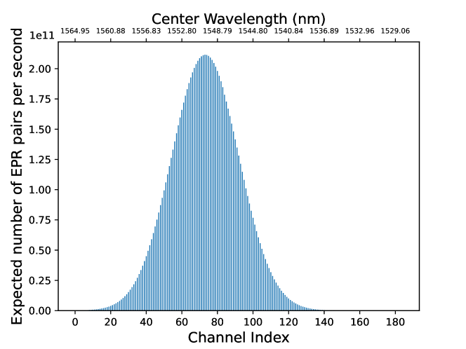
Figure 1: Rate of EPR-pair generation in $m=185$ channels of width 12.5 GHz, used for simple and ILEC networks. The bottom-axis label shows the channel indices and the top-axis label shows the center wavelength of each channel.

III-A Broadband Degenerate EPR-pair Generation

We assume the availability of a broadband, quasi-deterministic EPR-pair source. An example of such is the zero-added loss entangled multiplexing (ZALM) scheme described in [3]. It employs dual spontaneous parametric down-conversion (SPDC) processes, taking advantage of their broadband output. ZALM heralds polarization-entangled photon pairs in time and frequency via the following wavelength-demultiplexed Bell state measurement: the idler photons generated by both SPDC processes are interfered at a beamsplitter, wavelength-demultiplexed, and photodetected. The photon coincidence counts occurring at the same wavelength for two idler photons then herald entanglement of the signal photons. The corresponding heralded signal photons of now known and identical wavelength are directed through a WDM system with wavelength-selective add-drop capability.

We assume a conventional SPDC source that produces entangled photons at the rate that follows a Gaussian function centered at 1550 nm with a full-width half max of 9 nm. We divide the spectrum which falls within the C-band (1528-1565 nm or 191.69-196.33 THz) into $m$ channels of equal widths in frequency. Channels are separated by a gap equal to the channel width to prevent fidelity loss from wavelength ambiguity. We discuss the selection of the number of channels, $m$, and channel width in Section III-D.

Due to the Gaussian output spectrum from the SPDC sources, the EPR-pair generation rate per second for channels near 1550 nm is higher than for those on the edges of the spectrum. The EPR-pair source is depicted in Fig. 2a as ‘Source Node A.’ Note that our analysis can be adapted to other methods of generating degenerate EPR-pairs. The output spectrum from this source can be routed and distributed across the network using WDM routing techniques like those that have been developed for classical optical networks [4].

III-B Node Architecture

Each photon of the generated EPR-pair is directed by the source into a separate fiber. The node is built around $1\times N$ WSSs, whose role is to route wavebands towards different consumer nodes or else towards its own quantum memory bank. These wavebands group the source wavelength channels, e.g., those depicted in Fig. 1. Information heralded by the EPR-pair generation process (including the channel and timestamp of the generated pair) is transmitted along a classical network that is not depicted here. A consumer node lacks EPR-pair generation capability but has all the other components of the source node. The block diagrams for both the source and consumer nodes are in Fig. 2a.

Measured insertion loss $l_{\text{WSS}}$ on Lumentum’s TrueFlex Twin WSS ranges from 4 dB to 8 dB [23]. Hence we analyze EPR-pair distribution for two values of WSS loss: $l_{\text{WSS}}\in\{4,8\}$ dB. While they add significant loss, we note that WSSs are currently manufactured for use in classical networks and, thus, are not optimized for loss reduction. Other wavelength management and switching devices can achieve a loss of 2 dB [24]. Here we employ wavelength-independent loss $l$ in dB that is related to power transmittance by $\eta=10^{-l/10}$.

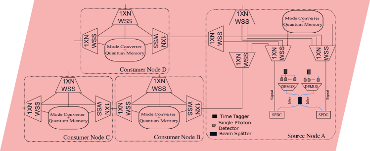
(a) Network Layout

(b) Graph Model

Figure 2: Correspondence between a network layout and its graph model. LABEL:sub@fig:source_consumer_network_model shows a network of source (A) and consumer nodes (B, C, and D). LABEL:sub@fig:source_consumer_graph_model shows the corresponding graph model.

III-C Network Topologies

We analyze the topology model of an existing incumbent local exchange carrier (ILEC) node map of Manhattan [8, 9]. This topology contains $n=17$ ILEC sites, with each site connected to between 2 and 16 other nodes. The layout of these nodes is shown in Fig. 3. While this is the reference topology for validating the performance of our approximation algorithms, the comparison with an optimal ILP solution is restricted to a smaller network topology with $n=6$ nodes, shown in Fig. 4, because the optimal fair allocation of EPR-pairs is an NP-hard problem.

Additionally, we study the impact of network size on the performance by employing random Watts-Strogatz graphs [10]. These are generated as follows: first, $n$ nodes are generated and connected to their $k$ nearest neighbors symmetrically in a ring. Then, for every node, each edge connected to $k/2$ rightmost neighbors is rewired with probability $\beta$ to a different, randomly chosen node. These graphs are useful in network science due to their small-world properties. We consider the parameters $n\in\{10,20,30,40\}$, $\beta\in\{0.2,0.5,0.8\}$, and $\frac{k}{n}\in\bigl{\{}\frac{1}{5},\frac{2}{5},\frac{3}{5},\frac{4}{5}\bigl{\}}$.

III-D Channelization

We utilize channel widths of 12.5 GHz for both the ILEC and simple topologies, yielding a $m=185$ channels, as illustrated in Fig. 1. Thus, the lowest and highest indexed channels correspond to center frequencies of 191.17 THz and 196.29 THz. For larger Watts-Strogatz networks $m=185$ channels are insufficient, because each of $\kappa=\binom{n}{2}=n(n-1)/2$ node pairs needs to be assigned at least one channel. We use $m=\lfloor 1.36\binom{n}{2}\rfloor$ where $1.36$ is the number of channels per node pair available in the ILEC network: $185/\binom{17}{2}=1.36$. This results in channel widths of 38 GHz when analyzing Watts-Strogatz graphs with $n=10$ and 2.19 GHz with $n=40$. We denote by $\bar{n}_{x}$ the EPR-pair rate generated in channel $x$. We adjust the total available EPR-pair rate $\sum_{x=1}^{m}\bar{n}_{x}$ across differently-sized Watts-Strogatz topologies to maintain a constant ratio $\frac{1}{\kappa}\sum_{x=1}^{m}\bar{n}_{x}$. This allows a fair comparison among networks with varying $n$.

III-E Network Architecture

The deployed fiber link lengths between nodes in the ILEC topology depicted in Fig. 3 are unknown. Thus, we use direct ‘as the crow flies’ distance as a proxy. The fiber link lengths between nodes of the simple network are shown in Fig. 4. For Watts-Strogatz we set all fiber link lengths to 5 km.

Standard single-mode fiber is assumed on each link. We employ a higher loss coefficient of $\alpha=0.4$ dB/km than typical fiber loss at 1550 nm (found in, e.g.,[25]) to account for higher losses and longer run lengths characteristic of metro fiber plant. We assume that all node pairs in the network request EPR-pairs from the source. Each wavelength channel is assigned to a single pair. The wavelength routing mechanism follows a circuit-switching approach. The routes serving different sets of node pairs do not interfere with one another, however, photons from a particular channel cannot be directed to two different nodes of a pair via the same fiber in the same direction, as this results in a routing ambiguity. Therefore, we only consider networks that allow disjoint light-paths from the source to each of the $\kappa$ node pairs. Edge-disjoint paths can be absent only if the minimum cut of the graph is less than two. We eliminate such instances of random Watts-Strogatz topologies.

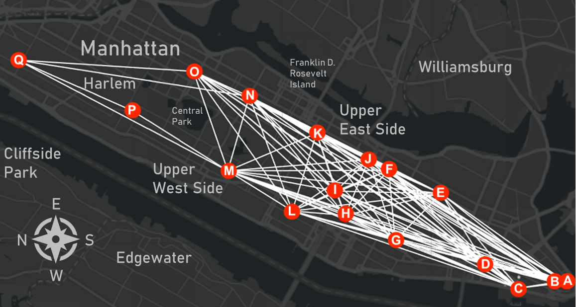
Figure 3: A map of Manhattan with ILEC nodes and links overlaid.

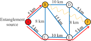
Figure 4: Topology of the simple network.

III-F Network Model

We represent a network as a graph denoted by $\mathcal{G}=(\mathcal{V},\mathcal{E})$, where $\mathcal{V}$ and $\mathcal{E}$ are the sets of vertices and directed edges, respectively. We also define a map $w:\mathcal{E}\to\mathbb{R}$ that assigns photon losses (in dB) as edge weights. We construct $\mathcal{G}$ for the network topologies described in Section III-C as follows:

• For each pair $(i,j)$ of connected consumer nodes we add the following directed edges and the corresponding vertices: $e^{i,\text{out}_{j}}_{j,\text{in}_{i}}\equiv\left(v_{i,\text{out}_{j}},v_{j,\text{in}_{i}}\right)$ and $e^{j,\text{out}_{i}}_{i,\text{in}_{j}}\equiv\left(v_{j,\text{out}_{i}},v_{i,\text{in}_{j}}\right)$ to $\mathcal{G}$. Hence each vertex is indexed by the node it belongs to, and by the role of that vertex. Vertices that serve input/output roles have the name of the corresponding external node as a subscript. The weight of the edges is $w\left(e^{i,\text{out}_{j}}_{j,\text{in}_{i}}\right)=w\left(e^{j,\text{out}_{i}}_{i,\text{in}_{j}}\right)=\alpha\times d(i,j)$, where $d(i,j)$ is the distance (in km) between nodes $i$ and $j$, and $\alpha$ is optical fiber loss (in dB/km) discussed in Section III-E.

• For each consumer node $i$, we iterate over all nodes $j,k$ that connect to $i$, and add edges $e^{i,\text{in}_{j}}_{i,\text{out}_{k}}\equiv\left(v_{i,\text{in}_{j}},v_{i,\text{out}_{k}}\right)$ to $\mathcal{E}$. This captures the consumer nodes’ internal connections between incoming and outgoing ports. Since the photons routed through a consumer node must traverse two WSSes, the weight of these edges is $w\left(e^{i,\text{in}_{j}}_{i,\text{out}_{k}}\right)=2l_{\rm WSS}$, as discussed in Section III-E. Furthermore, we also add edges $e^{i,\text{in}_{j}}_{i,\text{mem}}\equiv\left(v_{i,\text{in}_{j}},v_{i,\text{mem}}\right)$ describing internal connections to node $i$’s quantum memory to $\mathcal{E}$, and the corresponding vertices to $\mathcal{V}$. Since only one WSS is traversed in this case, $w\left(e^{i,\text{in}_{j}}_{i,\text{mem}}\right)=l_{\rm WSS}$.

• For the source node $s$, we iterate over all nodes $j$ that connect to $s$, and add edges $e^{s,\text{out}_{j}}_{j,\text{in}_{s}}\equiv\left(v_{s,\text{out}_{j}},v_{j,\text{in}_{s}}\right)$ to $\mathcal{E}$ and corresponding vertices to $\mathcal{V}$. The weight of these edges is $w\left(e^{s,\text{out}_{j}}_{j,\text{in}_{s}}\right)=\alpha\times d(s,j)$. Consumer node’s incoming vertices $v_{j,\text{in}_{s}}$ are connected to outgoing vertices and quantum memories as described above. Finally, we add edges $e^{s,\text{gen}}_{s,\text{out}_{j}}\equiv\left(v_{s,\text{gen}},v_{s,\text{out}_{j}}\right)$ and $e^{s,\text{gen}}_{s,\text{mem}}\equiv\left(v_{s,\text{gen}},v_{s,\text{mem}}\right)$ from vertex $v_{s,\text{gen}}$ describing EPR-pair generator to all outgoing ports and vertex $v_{s,\text{mem}}$ describing source’s own quantum memory. The weights for these edges are $w\left(e^{s,\text{gen}}_{s,\text{out}_{j}}\right)=2l_{\rm WSS}$ and $w\left(e^{s,\text{gen}}_{s,\text{mem}}\right)=l_{\rm WSS}$, per above. Note that the source node does not have incoming ports.

The total loss on a path from source to a consumer node $i$ is the sum of weights of the edges connecting $v_{s,\text{gen}}$ to $v_{i,\text{mem}}$. Fig. 2b depicts a graph model corresponding to the four-node network shown in Fig. 2a.

III-G Max-min (Egalitarian) Fairness

We seek max-min, or egalitarian, fairness, and maximize the minimum rate of EPR-pairs received by all $\kappa=n(n-1)/2$ pairs $(i,j)$ of $n$ nodes [26]. Let $l_{(i,j)}$ be the total loss (in dB) from the source to nodes $(i,j)$. That is, $l_{(i,j)}$ is the sum of losses on the disjoint paths from source to nodes $i$ and $j$, per Section III-F. Then, transmittance $\eta_{(i,j)}=10^{-l_{(i,j)}/10}$ is the fraction of the entangled photon pairs that are received by $(i,j)$. Let $\mathcal{A}_{(i,j)}$ be the set of channels assigned to node pair $(i,j)$. Since each channel cannot be assigned to more than one node pair, the set $\mathcal{P}=\left\{\mathcal{A}_{(i,j)}:i,j=1,\ldots,n,i\neq j\right\}$ partitions the $m$ available channels. Let $\bar{n}_{x}$ be the EPR-pair rate generated in channel $x$. The EPR-pair rate received by node pair $(i,j)$ is then $\bar{n}_{(i,j)}=\eta_{(i,j)}\sum_{x\in\mathcal{A}_{(i,j)}}\bar{n}_{x}$ and the max-min fair allocation involves the following optimization: $\max_{\mathcal{P}}\min_{(i,j)}\bar{n}_{(i,j)}$.

IV Algorithms

Orthogonality of sets $\mathcal{A}_{(i,j)}$ allows treating routing and spectrum allocation problems separately, as discussed next.

IV-A Optimal routing

Unlike standard networks, our source-in-the-middle entanglement distribution system described in Section III requires two disjoint light paths from source $s$ to nodes $i$ and $j$ that minimize total loss $l_{(i,j)}$ for each pair $(i,j)$ in the network. Per Section III-F, this translates to finding edge-disjoint routes in $\mathcal{G}$ from $v_{s,\text{gen}}$ to $v_{i,mem}$ and $v_{j,\text{mem}}$ minimizing the sum of weights of these paths. To this end, we use Suurballe’s algorithm [5, 6] as follows: for each consumer pair $(i,j)$ we add a dummy vertex $v_{(i,j),\text{d}}$ to $\mathcal{V}$ and dummy zero weighted edges: $e^{i,\text{mem}}_{(i,j),\text{d}}\equiv\left(v_{i,\text{mem}},v_{(i,j),\text{d}}\right)$ and $e^{j,\text{mem}}_{(i,j),\text{d}}\equiv\left(v_{j,\text{mem}},v_{(i,j),\text{d}}\right)$ to $\mathcal{E}$. Suurballe’s algorithm yields two edge-disjoint paths of minimum total weight between $v_{s,\text{gen}}$ and $v_{(i,j),\text{d}}$. Removing dummy vertices and edges returns edge-disjoint paths of minimum total weight from $v_{s,\text{gen}}$ to $v_{i,mem}$ and $v_{j,\text{mem}}$ for all pairs $(i,j)$. Suurballe’s algorithm’s run-time is polynomial in graph size.

IV-B Spectrum Allocation Strategies

Let $X$ be an $m\times\kappa$ binary matrix with $X_{x,(i,j)}=1$ if channel $x$ is assigned to node pair $(i,j)$ and zero otherwise (note that the pair $(i,j)$ indexes columns of $X$). Formally, $X_{x,(i,j)}=\left\{1~{}\text{if}~{}x\in\mathcal{A}_{(i,j)};0~{}\text{else}\right\}$. Also define an $\kappa\times\kappa$ diagonal matrix $\Lambda$ with transmittances $\eta_{(i,j)}^{\ast}$ of optimal routes (see Section IV-A) from source to each node pair $(i,j)$ on the diagonal and a vector $N=\left[\bar{n}_{1},\ldots,\bar{n}_{m}\right]$ of EPR-pair-generation rates in each channel (see Section III-G). For some $X$, the rate of EPR-pairs received by $(i,j)$ is $\bar{n}_{(i,j)}=\left[NX\Lambda\right]_{(i,j)}$, the $(i,j)^{\text{th}}$ entry of vector $NX\Lambda$. Finding an optimal spectrum allocation matrix $X$ is a well-known problem in optical networking [7]. Here we focus on maintaining max-min fairness in source-in-the-middle entanglement distribution.

IV-B1 Optimal Assignment

The following integer linear program (ILP) yields the optimal max-min fair solution:

$$\max_{X}T\text{~{}s.t.~{}} \sum_{\genfrac{}{}{0.0pt}{}{i,j=1}{i\neq j}}^{n}X_{x,(i,j)}=1,\forall x=1,\ldots,m$$ (1a)

$$\left[NX\Lambda\right]_{(i,j)}\geq T,\forall i,j=1,\ldots,n,i\neq j,$$ (1b)

where constraint (1a) enforces that each channel is assigned only once and (1b) ensures that each node pair receives EPR-pair rate of at least $T$.

The routing scheme in our scenario implicitly enforces wavelength contiguity constraints, as wavelengths cannot be switched at intermediate nodes. This contrasts with classical optical networks, where optimal spectrum allocation has to explicitly enforce them. Additionally, unlike classical networks that allow fractional channel allocation, source-in-the-middle entanglement distribution requires discrete channel assignment to entangle two particular quantum memories. This necessitates solving an NP-hard ILP problem. Hence, we consider approximations.

IV-B2 Round Robin [27]

Consumer node pairs, sorted in descending order of loss, are assigned channels in a cyclic order. The available channel with the highest EPR-pair rate is selected at each step. Algorithm 1 provides the pseudocode. The time complexity of this algorithm is determined by sorting the $\kappa$ node pairs and $m$ channels. Since $m\geq\kappa$, the overall time complexity is $\mathcal{O}(m\log{m})$.

1:procedure RoundRobin($\Lambda,N$)

2:     $nr\leftarrow\Lambda.diagonal.length$ $\triangleright$ Number of node pairs

3:     $nc\leftarrow N.length$ $\triangleright$ Number of channels

4:     $X\leftarrow\textsc{zeros}(nc,nr)$

5:     $\eta\leftarrow\Lambda.diagonal$ $\triangleright$ Transmittances

6:     $\hat{\eta},I_{\eta}\leftarrow\textsc{SortAscending}(\eta)$

7:     $\triangleright$ $\hat{\eta}$ has the transmittance in ascending order, $I_{\eta}$ has indices of the sorted array in the original array

8:     $\hat{N},I_{N}\leftarrow\textsc{SortDescending}(N)$ $\triangleright$ As previous line, but in descending order

9:     $i\leftarrow 0$ $\triangleright$ Tracks channel index at current iteration

10:     while $i<nc$ do

11:         $j\leftarrow i\bmod nr$ $\triangleright$ next lowest transmittance picks the next highest channel

12:         $X[I_{N}[i],I_{\eta}[j]]\leftarrow 1$

13:         $i\leftarrow i+1$

14:     end while

15:     return $X$

16:end procedure

Algorithm 1 Round Robin

IV-B3 First Fit [7]

We assign channels sequentially to a node pair. If EPR-pair rate $T$ is reached, then we repeat for the next node pair. The ordering of consumer node pairs follows a descending order based on loss. We restart with a smaller $T$ if channels are exhausted before all node pairs attain EPR-pair rate $T$. The maximum value $T^{\ast}$ satisfied by this algorithm can be found via binary search. Algorithm 2 provides the pseudocode. Its time complexity is $\mathcal{O}\left(m\log\left({\frac{1}{\kappa}\sum_{x=1}^{m}\bar{n}_{x}}\right)\right)$.

1:  

2:Main Procedure

3:  

1:procedure FirstFit($\Lambda,N$)

2:     $nr\leftarrow\Lambda.diagonal.length$ $\triangleright$ Number of node pairs

3:     $nc\leftarrow N.length$ $\triangleright$ Number of channels

4:     $\eta\leftarrow\Lambda.diagonal$ $\triangleright$ Transmittances

5:     $\hat{\eta},I_{\eta}\leftarrow\textsc{SortAscending}(\eta)$ $\triangleright$ $\hat{\eta}$ has the transmittance in ascending order, $I_{\eta}$ has indices of the sorted array in the original array

6:     $T^{\ast}\leftarrow\textsc{BinarySearch}(low=0,high=\lceil{\frac{sum(N)}{nr}}\rceil,predicate=FirstFitPredicate)$

7:     $X,\_\leftarrow\textsc{FirstFitAssignment}(T^{\ast})$

8:     return $X$

9:end procedure

1:  

2:Auxiliary procedures inheriting context from the main procedure

3:  

1:procedure FirstFitAssignment($T$)

2:     $X\leftarrow\textsc{zeros}(nc,nr)$

3:     $A\leftarrow\textsc{zeros}(1,nr)$ $\triangleright$ Stores Assigned EPR-pair rates for each node pair

4:     $i\leftarrow 0$ $\triangleright$ Tracks channel index

5:     $j\leftarrow 0$ $\triangleright$ Tracks node pair index

6:     while $i<nc\And j<nr$ do

7:         $\hat{j}\leftarrow I_{\eta}[j]$ $\triangleright$ Node pair’s index in unsorted list

8:         $X[i,\hat{j}]\leftarrow 1$

9:         $i\leftarrow i+1$

10:         $A[\hat{j}]=A[\hat{j}]+\hat{\eta}[j]N[i]$

11:         if $A[\hat{j}]\geq T$ then

12:              $j\leftarrow j+1$

13:         end if

14:     end while

15:     return $X,A$

16:end procedure

17:procedure FirstFitPredicate($T$)

18:     $\_,A\leftarrow\textsc{FirstFitAssignment}(T)$

19:     for $j=0,\dots,(nr-1)$ do

20:         if $A[j]<T$ then

21:              return false

22:         end if

23:     end for

24:     return true

25:end procedure

Algorithm 2 First Fit

IV-B4 Modified Longest Processing Time First (LPT) [28, 29]

This is a well-known machine scheduling algorithm. We modify it to greedily optimize for the max-min rather than min-max goal, akin to [30]: each channel is assigned to a node pair which maximizes the current minimum received EPR-pair rate across the node pairs. While our experiments indicate that this approach performs well, we have not derived any analytical performance guarantees. The pseudocode for this algorithm is given in Algorithm 3. Its time complexity is determined by sorting the $\kappa$ node pairs and $m$ channels, and finding the minimum value of $\kappa$ node pairs for $m-\kappa$ iterations. The time required for sorting the node pairs can be disregarded, as in the analysis of the Round Robin algorithm. Hence the overall time complexity is given as $\mathcal{O}(m\kappa+m\log m)$.

1:procedure ModifiedLPT($\Lambda,N$)

2:     $nr\leftarrow\Lambda.diagonal.length$ $\triangleright$ Number of node pairs

3:     $nc\leftarrow N.length$ $\triangleright$ Number of channels

4:     $X\leftarrow\textsc{zeros}(nc,nr)$

5:     $\eta\leftarrow\Lambda.diagonal$ $\triangleright$ Transmittances

6:     $\hat{\eta},I_{\eta}\leftarrow\textsc{SortAscending}(\eta)$ $\triangleright$ $\hat{\eta}$ has the transmittance in ascending order, $I_{\eta}$ has indices of the sorted array in the original array

7:     $\hat{N},I_{N}\leftarrow\textsc{SortDescending}(N)$ $\triangleright$ As previous line, but in descending order

8:     $A\leftarrow\textsc{zeros}(1,nr)$ $\triangleright$ Stores assigned EPR-pair rates for each node pair

9:     $\triangleright$ Assign each node pair one channel

10:     for $j=0,\dots,(nr-1)$ do

11:         $X[I_{N}[j],I_{\eta}[j]]\leftarrow 1$

12:         $A[I_{\eta}[j]]=A[I_{\eta}[j]]+\hat{\eta}[j]\hat{N}[j]$

13:     end for

14:     $\triangleright$ Now assign each new channel greedily

15:     $i\leftarrow nr$

16:     while $i<nc$ do

17:         $j\leftarrow\textsc{ArgMin}(A)$

18:         $X[I_{N}[i],j]\leftarrow 1$

19:         $A[j]\leftarrow A[j]+\eta[j]\hat{N}[i]$

20:         $i\leftarrow i+1$

21:     end while

22:     return $X$

23:end procedure

Algorithm 3 Modified LPT

IV-B5 Bezáková and Dani’s $1/(m-k+1)$-approximation (BD) [31]

This iterative polynomial-time algorithm converges to a solution that is guaranteed to be within $1/(m-k+1)$ of the optimal max-min EPR-pair rate. We make two modifications: 1) instead of always assigning one channel to each node pair in each round, we allow skipping a channel assignment; 2) in each round, we prefer the assignment which minimizes the total rate of EPR-pair generation that is assigned. These are invoked as long as it does not impact the overall max-min EPR-pair rate, hence they can only increase the minimum received EPR-pair rate for all node pairs, all the while preserving the original approximation guarantee. The pseudocode for this algorithm is given in Algorithm 4. It assigns each node pair one channel in the first round, and zero or one channels in subsequent rounds, and thus has to run for $m-\kappa+1$ rounds in the worst case. In each round, we run a binary search taking a maximum of $\log(\max(N))$ iterations. For each run, the maximum matching can be found in $\mathcal{O}(m\kappa(m+\kappa)+(m+\kappa)^{2})$ time using the Ford-Fulkerson algorithm [32]. Finally, finding the minimum-weight matching is found in $\mathcal{O}(\kappa\log(\kappa)+m\kappa)$ time. This results in the total time complexity of $\mathcal{O}(g(m,\kappa))$, where

$$g(m,\kappa) =(\log(\max(N))(m\kappa(m+\kappa)+(m+\kappa)^{2})+\kappa\log(\kappa)m)$$

$$\phantom{=}\times(m-\kappa+1),$$ (2)

which simplifies to $\mathcal{O}(m^{3}\kappa\log(\max(N)))$.

1:  

2:Main Procedure

3:  

1:procedure BD($\Lambda,N$)

2:     $nr\leftarrow\Lambda.diagonal.length$ $\triangleright$ Number of node pairs

3:     $nc\leftarrow N.length$ $\triangleright$ Number of channels

4:     $X\leftarrow$ array of zeros of size $nr\times nc$ $\triangleright$ Note the order of dimensions

5:     $\eta\leftarrow\Lambda.diagonal$

6:     $\mathcal{G}\leftarrow$ BipartiteGraph($\eta,N$)

7:     $T^{\ast}\leftarrow 0$

8:     while $\text{length}(G.channels)\geq\text{length}(G.nodepairs)$ do

9:         $T^{\ast}\leftarrow\textsc{BinarySearch}(low=T^{\ast},high=T^{\ast}+\lceil{\frac{\text{sum}(N)}{nr}}\rceil,predicate=MatchingExists)$

10:         $\mathcal{G^{\prime}}\leftarrow$ MinWeightMatching($\mathcal{G},T^{\ast}$) $\triangleright$ The original algorithm uses any matching, not necessarily min-weight

11:         for all $e$ in $\mathcal{G^{\prime}}.edges$ do

12:              $node\_pair\leftarrow e.start$ $\triangleright$ Node pair vertex

13:              $channel\leftarrow e.end$ $\triangleright$ Channel vertex

14:              $node\_pair\_idx\leftarrow$ index of $node\_pair$ in $\eta$

15:              $channel\_idx\leftarrow$ index of $channel$ in $N$

16:              $X[channel\_idx,node\_pair\_idx]\leftarrow 1$ $\triangleright$ Mark the connection between node pair and channel

17:              $\mathcal{G}\leftarrow$ DeleteVertex($\mathcal{G},channel$)

18:              $node\_pair.weight\leftarrow node\_pair.weight+e.weight$ $\triangleright$ Update the weight of the node pair

19:         end for

20:     end while

21:     $\Lambda_{rel},N_{rel}\leftarrow$ ExtractRelevant($\Lambda,N,\mathcal{G}$) $\triangleright$ Extract relevant Lambdas and N

22:     $X\_RR\leftarrow$ RoundRobin($\Lambda_{rel},N_{rel}$) $\triangleright$ Assign unassigned channels in Round Robin manner

23:     $X\leftarrow X+X\_RR$ $\triangleright$ Combine assignments

24:     return $X$

25:end procedure

1:  

2:Auxiliary procedures inheriting context from the main procedure

3:  

1:procedure BipartiteGraph($\eta,N$)

2:     $\mathcal{G}.nodes\leftarrow\mathcal{G}.nodepairs\cup\mathcal{G}.channels$

3:     $n.weight\leftarrow 0,\quad\forall n\in\mathcal{G}.nodes$

4:     for $e$ in $\mathcal{G}.edges$ do

5:         $node\_pair\_idx\leftarrow$ index of $e.start$ in $\eta$

6:         $channel\_idx\leftarrow$ index of $e.end$ in $N$

7:         $e.weight\leftarrow\eta[channel\_idx]\times N[node\_pair\_idx]$ $\triangleright$ Calculate edge weight

8:     end for

9:     return $\mathcal{G}$

10:end procedure

11:procedure MatchingExists($G,T$)

12:     $\mathcal{\hat{G}}\leftarrow$ModifiedGraph($G$)

13:     return HasMatching($\mathcal{\hat{G}}$)

14:end procedure

15:procedure ModifiedGraph($G,T$)

16:     for $n$ in $G.nodes$ do $\triangleright$ Remove nodes that have at least $T$ weight

17:         if $n.weight\geq T$ then

18:              Remove $n$ from $G.nodes$

19:         end if

20:     end for

21:     for $e$ in $G.edges$ do $\triangleright$ Add node weights to edge weights

22:         $e.weight\leftarrow e.weight+e.start.weight$

23:     end for

24:     for $e$ in $G.edges$ do $\triangleright$ Prune edges whose weights represent less than T EPR-pair rate

25:         if $e.weight<T$ then

26:              Remove $e$ from $G.edges$

27:         end if

28:     end for

29:end procedure

30:procedure MinWeightMatching($G,T$)

31:     $\triangleright$ Assumes a matching exists

32:     $\mathcal{\hat{G}}\leftarrow$ModifiedGraph($G$)

33:     $R\leftarrow$ Sort node pairs in $\mathcal{\hat{G}}$ in descending order based on the following criteria:

34:      1. Number of neighboring channels

35:      2. Transmittance associated with each node pair

36:     for all $r$ in $R$ do

37:         Find the neighbors of node pair $r$, which are channels connected to $r$ (as $G$ is bipartite).

38:         Among these channels, identify the channel with the fewest photons.

39:         Let $c$ be this channel, and let $c_{i}$ be its index in the list $N$.

40:         Delete all edges in $\mathcal{\hat{G}}$ originating from $r$ that are not connected to $c$.

41:     end for

42:     return $\mathcal{\hat{G}}$

43:end procedure

Algorithm 4 Modified BD

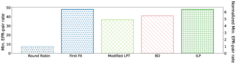
(a) Minimum received EPR-pair rates

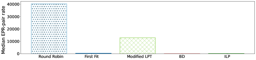
(b) Median received EPR-pair rates

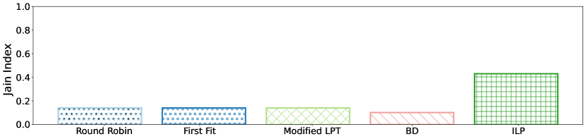
(c) Jain index

Figure 5: Comparison of performance using different allocation strategies on the simple network depicted in Fig. 4 for 8 dB WSS loss and source node location A. 5a shows unnormalized (left-axis label) and normalized (right-axis label) minimum EPR-pair rates received by any node pair.

(a)

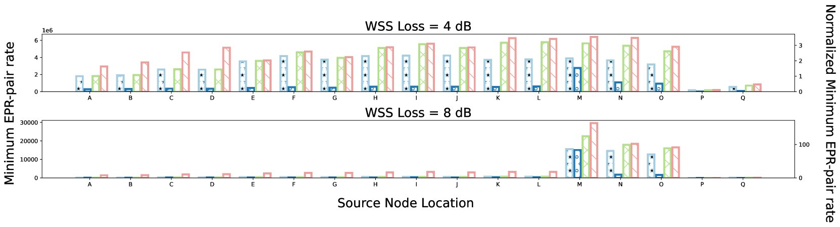
(a) Minimum received EPR-pair rates

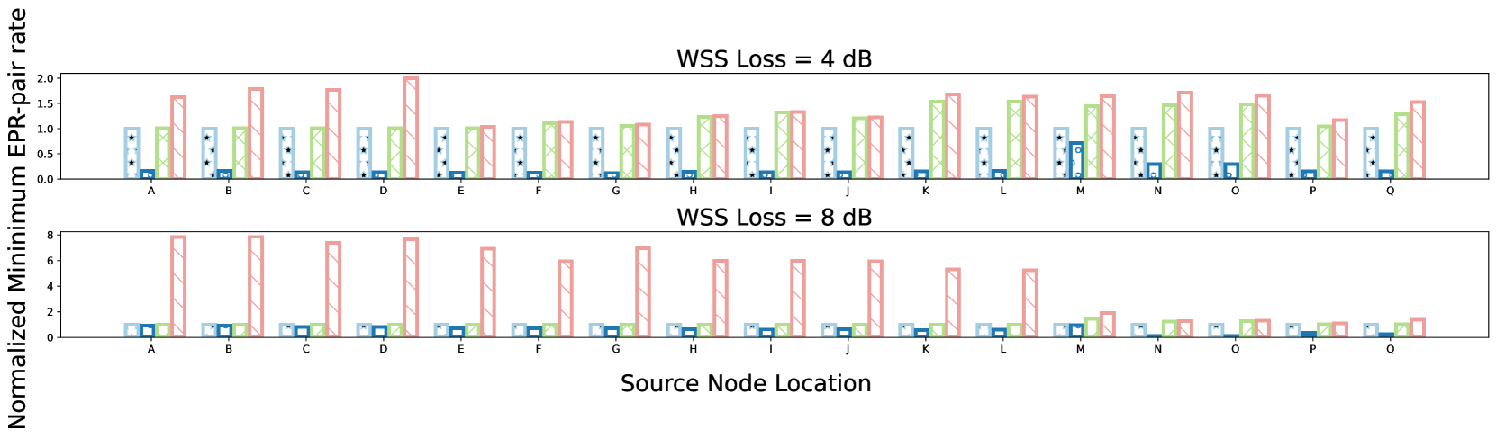
(b) Normalized Minimum received EPR-pair rates

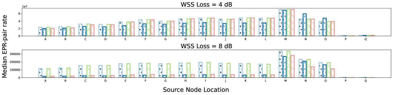
(c) Median received EPR-pair rates

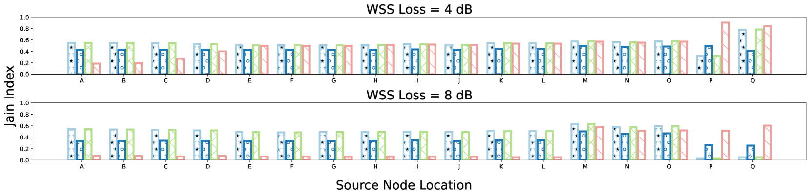
(d) Jain index

Figure 6: Comparison of performance using different allocation strategies on the ILEC network depicted in Fig. 3 for 4 dB and 8 dB WSS loss.

V Results and Discussion

V-A Metrics and Methods

For each of these networks, we analyze the minimum and median received EPR-pair rate, and the fairness in the allocation of these EPR-pairs. The minimum EPR-pair rate reflects the guaranteed rate to each node pair in the network. The median EPR-pair rate reflects the rate to at least half of the node pairs. We chose median over a mean to reduce impact from the exponential relationship between path length and transmission success probability. We also analyze the performance of the normalized minimum EPR-pair rates, which enables a comparison of allocation strategies across network configurations. Our normalization is relative to a baseline, which is the minimum EPR-pair rate assigned by Round Robin. It is used since it is a well-known and intuitive strategy.

The fairness of EPR rate allocation is quantified by the Jain index [33]. The Jain index for values $x_{i},i=1,\ldots,r$, is:

$$J(x_{1},x_{2}...x_{r}) =\frac{(\sum_{i=1}^{r}x_{i})^{2}}{r\sum_{i=1}^{r}x_{i}^{2}}$$ (3)

The maximum Jain index is unity, which occurs when all $x_{i}$’s are equal. Hence, this indicates complete fairness. The minimum Jain index $\frac{1}{r}$ indicates a completely unfair resource allocation. In our case, for a network with $n$ nodes, $r$ is the number of node pairs $r=\kappa=n(n-1)/2$. The dependence of the Jain index on $n$ limits its use when comparing fairness between networks with different numbers of nodes. We also use the Jain index to analyze the importance of source node location by calculating it for the minimum EPR-pair rates assigned for each possible source node location. A smaller Jain index (lower-bounded by $1/n$) indicates increased source node location importance, since this is due to a larger variation in the minimum EPR-pair rate across the choices of source node location.

For simple and ILEC networks, we use the minimum and median EPR-pair rate, and the Jain index to analyze the performance of the different channel allocation strategies, for different choices of source node placement, and values of WSS loss. For the random Watts-Strogatz networks with a fixed WSS loss of 4dB, we analyze the impact of input parameters $n$, $k$, and $\beta$ on the minimum and median EPR-pair rates, and the Jain index using the modified LPT and BD approximation algorithms. Analysis is restricted to only these algorithms as these were the best strategies on the fixed networks. The minimum and median EPR-pair rates, and the Jain index, are calculated for the max-min-optimal source node for each of the two algorithms, and are averaged over 100 randomly generated Watt-Strogratz topologies for each value of input parameters $n$, $k$, and $\beta$ given in Section III-C.

V-B Spectrum Allocation in Simple and ILEC Networks

Fig. 5a depicts the minimum EPR-pair rates received by any node pair in the simple network topology depicted in Fig. 4 when placing the source at node A and a WSS loss of 8 dB. We can calculate the optimal max-min solution using ILP for this configuration. We note that the BD approximation algorithm is close to optimal. Modified LPT and First Fit algorithms perform well; the First Fit’s performance is surprising given its relative simplicity. Round Robin performs poorly.

Fig. 5b depicts the median EPR-pair rates for the simple topology. ILP, which gave us the theoretical best performance on the minimum EPR-pair metric, shows poor performance on this metric. This behavior is also true for the BD and First Fit algorithms. Round Robin, which performed poorly on the minimum EPR-pair metric shows the best performance here, followed by modified LPT.

Fig. 5c examines the Jain index for the simple topology. Although the ILP algorithm consistently produces the same minimum EPR-pair rate in each run, it may use distinct assignment configurations, resulting in varying Jain index. Thus, the results from the ILP algorithm are averaged over 1000 runs, with each run randomizing the order of processing the node pairs. The confidence intervals are negligibly small and are not depicted. The ILP solution, which optimizes for the minimum received EPR-pair rate, also performs the best on this fairness measure. The performance of the other strategies is comparable to each other. The BD approximation algorithm, which performed well for minimum received EPR-pair rate, performs the poorest on the Jain index.

The variability in the performance of channel assignment algorithms on these metrics emphasizes the limitations inherent in each metric and underscores the importance of considering them collectively. While the minimum EPR-pair rate provides insights into the worst-case performance, it may not be representative of the majority of the rate allocations. Similarly, the median overlooks outliers in the allocation distribution. Additionally, the Jain index assesses the relative fairness among assignments but does not consider the magnitude of EPR-pair rates allocated.

Figs. 6a and  6b show the normalized and unnormalized minimum received EPR-pair rates in the ILEC network depicted in Fig. 3 for source at different network nodes. Due to the complexity of the ILP program for this topology, we cannot calculate the optimal solution. The number of intermediate nodes traversed by a path in the ILEC network varies significantly based on the source node location. A linear increase in the number of intermediate nodes traversed leads to an exponential decrease of the path transmittance. Hence we see that minimum EPR-pair rates vary significantly across source node locations. Also due to this exponential relationship between path loss in dB and transmittance, the difference in the minimum EPR-pair rates across source node locations is accentuated when the WSS loss is set to 8dB versus 4 dB.

The normalized values for the minimum EPR-pair rate indicate the relative performance improvement of a strategy compared to a trivial (Round Robin) strategy. This accentuates the superiority of BD approximation on ILEC topology for the WSS loss set to 8dB rather than 4 dB. Thus, a more careful approach in allocating channels that provide vastly different received EPR-pair rates can have significant benefit.

Consistent with findings for the simple network in Fig. 4, both the BD algorithm and modified LPT algorithms are effective in optimizing the minimum received ERP-pair rates by node pairs in ILEC network in Fig. 3. However, the First Fit algorithm, which performed well on the simple topology from Fig. 4, performs poorly here. This is due to the greater disparity in the transmittance to different node pairs in the ILEC network, owing to the greater difference in path losses to these node pairs. For the First Fit algorithm, scenarios can arise where no high EPR-pair rate channels are available by the time a node pair with highly lossy paths reaches its turn.

For different source locations, those with higher degrees can supply higher minimum EPR-pair rates. Nodes $A$ through $L$ have degree 14, and show similar performance. Node $M$ with the highest degree (16) demonstrates the best performance. Nodes $P$ and $Q$ have degrees two and four, respectively, and perform the poorest. Interestingly, the performance of nodes $N$ and $O$, which have degree 15, show dramatic improvement over nodes with degree 14. This can be attributed to the fact that these nodes’ neighbors are neighbors to node $Q$ and second-order neighbors to node $P$, the two nodes with smallest degree. Thus, while the nodes with 14 neighbors cannot efficiently supply EPR-pairs to node pairs containing $P$ or $Q$, source nodes $N$ and $O$ do not suffer from this.

Fig. 6c depicts the median EPR-pair rate in the ILEC network for the source at different network nodes. The median EPR-pair rates assigned by the channel assignment algorithms exhibit more comparable performance than the minimum EPR-pair rates. The BD algorithm, which demonstrated superior performance for the minimum EPR rate, does not perform as well as Round Robin and LPT on the median EPR rate metric.

Finally, Fig. 6d examines the Jain index for ILEC topology. The BD algorithm and LPT strategy perform best on this metric. The BD strategy is superior on source nodes $P$ and $Q$ when the WSS loss is 8 dB.

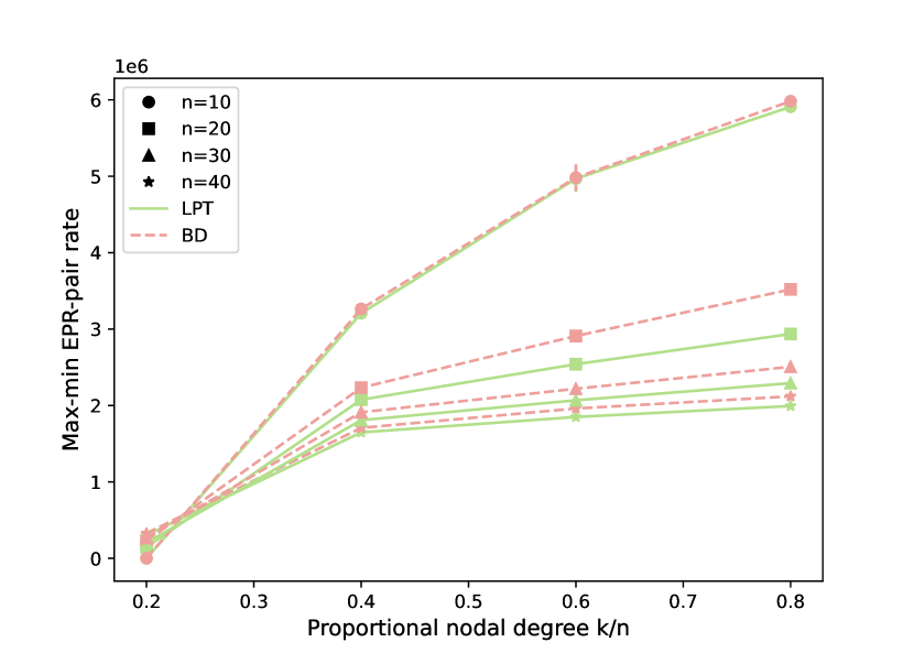
Figure 7: Max-min EPR-pair rates at the optimal source location for networks with varying number of nodes and proportional nodal degree. Rewiring probability $\beta=0.5$; results for other settings of $\beta$ are similar.

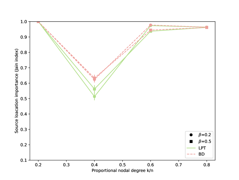
(a) $n=10$
Minimum Jain index = 0.1

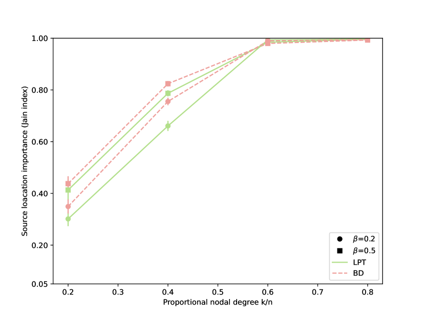
(b) $n=20$
Minimum Jain index = 0.05

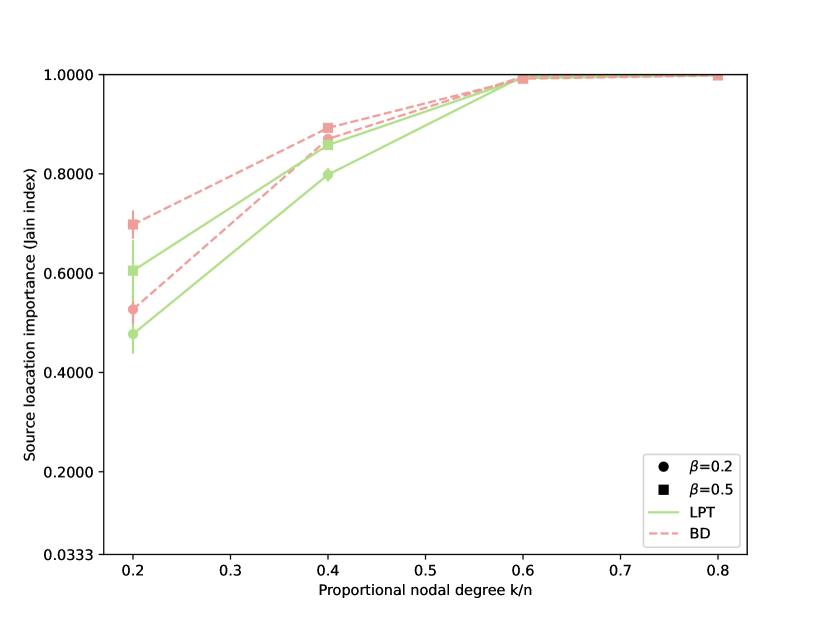
(c) $n=30$
Minimum Jain index = 0.0333

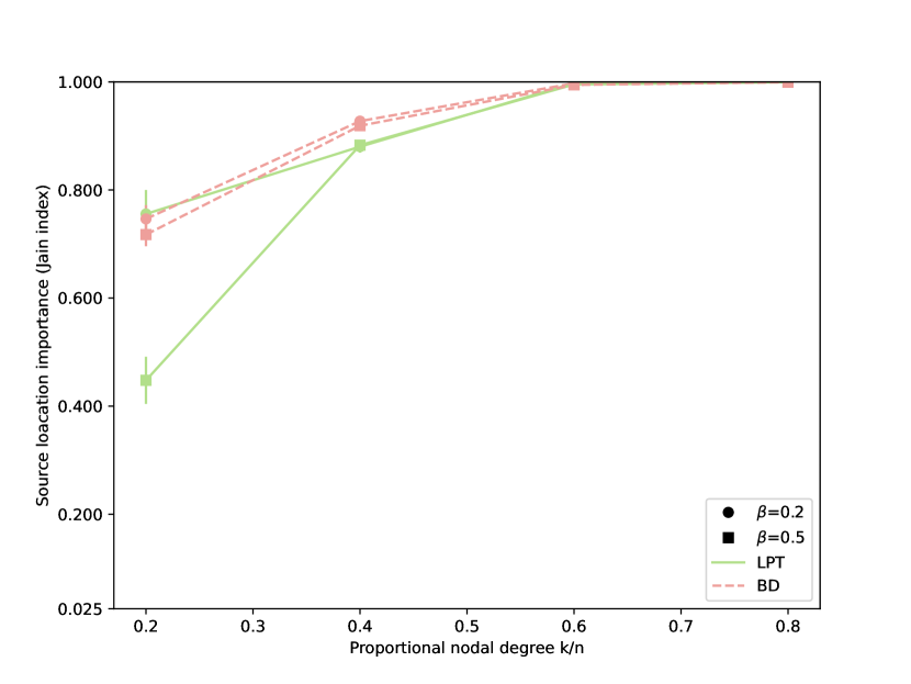
(d) $n=40$
Minimum Jain index = 0.025

Figure 8: Source node location importance measured using the Jain index for varying number of nodes, proportional nodal degree, and rewiring probability. Smaller Jain index indicates greater importance.

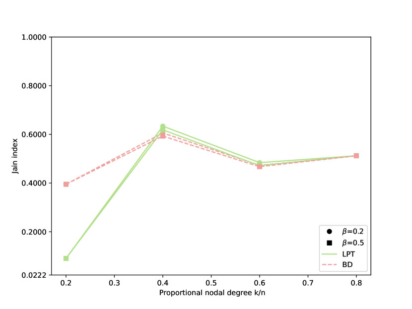
(a) $n=10$
Minimum Jain index = 0.0222

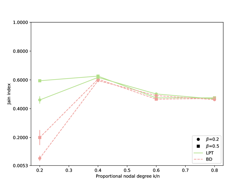
(b) $n=20$
Minimum Jain index = 0.0053

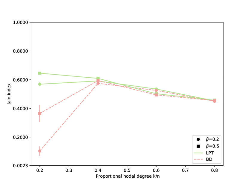
(c) $n=30$
Minimum Jain index = 0.0023

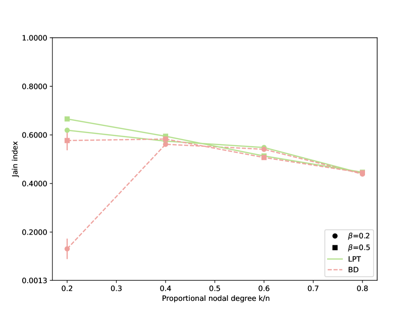
(d) $n=40$
Minimum Jain index = 0.0013

Figure 9: The fairness of the network and allocation strategy, measured using the Jain index at the node with the best max-min EPR-pair rate. Each subplot starts from its associated theoretical minimum value.

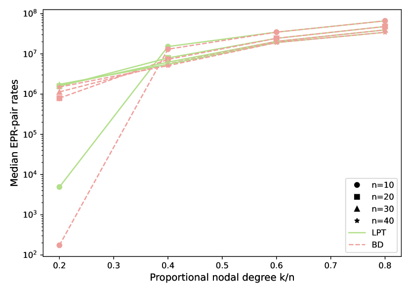
Figure 10: Median EPR-pair rates at the max-min-optimal source location for networks with varying number of nodes and proportional nodal degree. Rewiring probability $\beta=0.5$; results for other settings of $\beta$ are similar. Median EPR-pair rates on the ordinate are in log scale.

V-C Impact of Network Size and Connectivity

We analyze the impact of network size and connectivity using the Watts-Strogatz random networks described in Section III-C, We focus on modified LPT and BD approximation algorithms due to their superior performance over others. Fig. 7 shows that, as the number of nodes in a network increases, the minimum number of received EPR-pairs decreases. This is intuitive, as we expect that, with more nodes, the longer path lengths increase loss and decrease the likelihood that a photon successfully reaches its destination. Furthermore, as the proportional nodal degree $k/n$ increases, so does the minimum received EPR-pair rate. This is because increasing the number of connections in a network increases the possible available routing paths, thus, on average, decreasing the path lengths and loss in the best available paths. Finally, the rewiring probability $\beta$ does not seem to impact the max-min EPR-pair rate.

Next, we study the importance of source node location on the max-min received EPR-pair rate using the Jain index. Note that, for $n=10$ and $k=2$, varying the source node location does not impact the max-min EPR-pair rate because this corresponds to a rotationally-symmetric ring network, where each node is only connected to its neighbor. Fig. 8 shows that, as the proportional nodal degree increases, so does the importance of source location. This indicates an increasing uniformity of network path lengths. Additionally, for low-degree networks, the rewiring probability $\beta$ has a greater impact on the importance of source location. This is due to the fewer possible routes through the network.

Fig. 9 shows that, as proportional nodal degree $k/n$ increases, the spectrum allocation becomes less fair, indicated by a decrease in the Jain index. This is due to the combination of increasing uniformity in network path lengths driven by increasing $k/n$, and a highly non-uniform Gaussian dependence of the EPR-pair rates on the channels (see Section III-A).

Finally, we compare the median EPR-pair rates for the source node location optimizing the performance of BD and modified LPT algorithms in Fig. 10. Although these algorithms approximate an optimal max-min EPR-pair rate solution, median measures the impact of the choice of algorithm beyond the minimum rate. Consistent with minimum EPR-pair rate result in Fig. 7, the median EPR-pair rate decreases with increasing number of nodes. However, the modified LPT algorithm outperforms the BD algorithm in median EPR-pair rate, although the difference decreases with increasing $k/n$.

VI Conclusion

In this study, we explore the optimization of EPR-pair distribution in quantum networks to address the increasing demand for efficient quantum computation and communication. We consider a source-in-the-middle time-frequency-heralded architecture and examine optimal routing and various approaches for fair spectrum allocation that approximate the optimal NP-hard solution. For the latter, we find that the BD approximation and modified LPT algorithms outperform others in EPR-pair rate while being comparable to others in fairness as measured by the Jain index. Analysis of the modified LPT and BD approximation algorithms on the Watts-Strogatz networks, suggests that the latter outperforms the former in the minimum EPR-pair rate. However when including Jain index, median distribution of EPR-pair rates, and run time in the consideration, modified LPT outperforms BD approximation. Thus, determining the appropriate algorithm depends on which performance metrics are important to the intended application. Our future work will focus on algorithm refinement and experimental implementations. Furthermore, having multiple EPR-pair sources in a network substantially complicates the routing and spectrum allocation problem. We are exploring various approaches to address these.

References

- [1] R. Bali, A. Tittelbaugh, S. L. Jenkins, A. Agrawal, J. Horgan, M. Ruffini, D. Kilper, and B. A. Bash, “Routing and spectrum allocation in broadband degenerate epr-pair distribution,” in Proc. IEEE Int. Conf. Commun. (ICC), 2024.
- [2] A. Singh, K. Dev, H. Siljak, H. D. Joshi, and M. Magarini, “Quantum internet—applications, functionalities, enabling technologies, challenges, and research directions,” IEEE Commun. Surv. Tutor., vol. 23, no. 4, pp. 2218–2247, 2021.
- [3] K. C. Chen, P. Dhara, M. Heuck, Y. Lee, W. Dai, S. Guha, and D. Englund, “Zero-added-loss entangled-photon multiplexing for ground- and space-based quantum networks,” Phys. Rev. Appl., vol. 19, p. 054029, May 2023. [Online]. Available: https://link.aps.org/doi/10.1103/PhysRevApplied.19.054029
- [4] J. M. Simmons, Optical network design and planning. Springer, 2014.
- [5] J. Suurballe and R. Tarjan, “A quick method for finding shortest pairs of disjoint paths,” Networks, vol. 14, no. 2, pp. 325–336, 1984.
- [6] S. Banerjee, R. Ghosh, and A. Reddy, “Parallel algorithm for shortest pairs of edge-disjoint paths,” J. Parallel Distrib. Comput., vol. 33, no. 2, p. 165–171, Mar. 1996. [Online]. Available: https://doi.org/10.1006/jpdc.1996.0035
- [7] B. C. Chatterjee, N. Sarma, and E. Oki, “Routing and spectrum allocation in elastic optical networks: A tutorial,” IEEE Commun. Surv. Tutor., vol. 17, no. 3, pp. 1776–1800, 2015.
- [8] J. Yu, Y. Li, M. Bhopalwala, S. Das, M. Ruffini, and D. C. Kilper, “Midhaul transmission using edge data centers with split phy processing and wavelength reassignment for 5g wireless networks,” in 2018 Int. Conf. Opt. Netw. Des. Model. (ONDM), 2018, pp. 178–183.
- [9] Y. Li, M. Bhopalwala, S. Das, J. Yu, W. Mo, M. Ruffini, and D. C. Kilper, “Joint optimization of bbu pool allocation and selection for c-ran networks,” in 2018 Opt. Fiber Commun. Conf. Exhib. (OFC), 2018, pp. 1–3.
- [10] D. J. Watts and S. H. Strogatz, “Collective dynamics of ‘small-world’networks,” Nature, vol. 393, no. 6684, pp. 440–442, 1998. [Online]. Available: https://doi.org/10.1038/30918
- [11] S. Muralidharan, L. Li, J. Kim, N. Lütkenhaus, M. D. Lukin, and L. Jiang, “Optimal architectures for long distance quantum communication,” Sci. Rep., vol. 6, no. 1, p. 20463, 2016.
- [12] M. Pant, H. Krovi, D. Towsley, L. Tassiulas, L. Jiang, P. Basu, D. Englund, and S. Guha, “Routing entanglement in the quantum internet,” Npj Quantum Inf., vol. 5, no. 1, p. 25, 2019.
- [13] A. Patil, M. Pant, D. Englund, D. Towsley, and S. Guha, “Entanglement generation in a quantum network at distance-independent rate,” Npj Quantum Inf., vol. 8, no. 1, p. 51, 2022.
- [14] Y. Wang, X. Yu, Y. Zhao, A. Nag, and J. Zhang, “Pre-established entanglement distribution algorithm in quantum networks,” JIEEE J. Opt. Commun. Netw. (JOCN), vol. 14, no. 12, pp. 1020–1033, 2022.
- [15] N. K. Panigrahy, M. G. De Andrade, S. Pouryousef, D. Towsley, and L. Tassiulas, “Scalable multipartite entanglement distribution in quantum networks,” in 2023 IEEE Int. Conf. of Quantum Comput. Eng. (QCE), vol. 2. IEEE, 2023, pp. 391–392.
- [16] E. Kaur and S. Guha, “Distribution of entanglement in two-dimensional square grid network,” in 2023 IEEE Int. Conf. of Quantum Comput. Eng. (QCE), vol. 1. IEEE, 2023, pp. 1154–1164.
- [17] E. Sutcliffe and A. Beghelli, “Multi-user entanglement distribution in quantum networks using multipath routing,” IEEE Trans. Quantum Eng. (TQE), 2023.
- [18] E. A. Van Milligen, E. Jacobson, A. Patil, G. Vardoyan, D. Towsley, and S. Guha, “Entanglement routing over networks with time multiplexed repeaters,” arXiv preprint arXiv:2308.15028, 2023.
- [19] W. Chen, Z.-F. Han, T. Zhang, H. Wen, Z.-Q. Yin, F.-X. Xu, Q.-L. Wu, Y. Liu, Y. Zhang, X.-F. Mo, Y.-Z. Gui, G. Wei, and G.-C. Guo, “Field experiment on a “star type” metropolitan quantum key distribution network,” IEEE Photon. Technol. Lett., vol. 21, no. 9, pp. 575–577, 2009.
- [20] S. Wengerowsky, S. K. Joshi, F. Steinlechner, H. Hübel, and R. Ursin, “An entanglement-based wavelength-multiplexed quantum communication network,” Nature, vol. 564, no. 7735, pp. 225–228, 2018. [Online]. Available: https://doi.org/10.1038/s41586-018-0766-y
- [21] E. Y. Zhu, C. Corbari, A. Gladyshev, P. G. Kazansky, H.-K. Lo, and L. Qian, “Toward a reconfigurable quantum network enabled by a broadband entangled source,” J. Opt. Soc. Am. B, vol. 36, no. 3, pp. B1–B6, Mar. 2019. [Online]. Available: https://opg.optica.org/josab/abstract.cfm?URI=josab-36-3-B1
- [22] R. Wang, O. Alia, M. J. Clark, S. Bahrani, S. K. Joshi, D. Aktas, G. T. Kanellos, M. Peranić, M. Lončarić, M. Stipčević, J. Rarity, R. Nejabati, and D. Simeonidou, “A dynamic multi-protocol entanglement distribution quantum network,” in 2022 Opt. Fiber Commun. Conf. Exhib. (OFC), 2022, pp. 1–3.
- [23] TrueFlex® Twin High Port Count Wavelength Selective Switch (Twin WSS), Lumentum Holdings Inc, 11 1997, revised Sept. 2002.
- [24] P. D. Colbourne, S. McLaughlin, C. Murley, S. Gaudet, and D. Burke, “Contentionless twin 8×24 wss with low insertion loss,” in 2018 Opt. Fiber Commun. Conf. Exhib. (OFC), 2018, pp. 1–3.
- [25] “Optical loss & testing overview — kingfisher international.” https://kingfisherfiber.com/application-notes/optical-loss-testing-overview, accessed: Oct. 11, 2023.
- [26] R. J. Lipton, E. Markakis, E. Mossel, and A. Saberi, “On approximately fair allocations of indivisible goods,” in Proceedings of the 5th ACM Conference on Electronic Commerce, ser. EC ’04. New York, NY, USA: Association for Computing Machinery, 2004, p. 125–131. [Online]. Available: https://doi.org/10.1145/988772.988792
- [27] H. Aziz, I. Caragiannis, A. Igarashi, and T. Walsh, “Fair allocation of indivisible goods and chores,” Auton. Agents and Multi-Agent Syst., vol. 36, no. 1, p. 3, 2021. [Online]. Available: https://doi.org/10.1007/s10458-021-09532-8
- [28] R. L. Graham, “Bounds on multiprocessing timing anomalies,” SIAM J. Appl. Math., vol. 17, no. 2, pp. 416–429, 1969. [Online]. Available: http://www.jstor.org/stable/2099572
- [29] B. L. Deuermeyer, D. K. Friesen, and M. A. Langston, “Scheduling to maximize the minimum processor finish time in a multiprocessor system,” SIAM J. Algebr. Discrete Methods, vol. 3, no. 2, pp. 190–196, 1982. [Online]. Available: https://doi.org/10.1137/0603019
- [30] B. Y. Wu, “An analysis of the lpt algorithm for the max–min and the min–ratio partition problems,” Theor. Comput. Sci., vol. 349, no. 3, pp. 407–419, 2005. [Online]. Available: https://www.sciencedirect.com/science/article/pii/S0304397505005815
- [31] I. Bezáková and V. Dani, “Allocating indivisible goods,” SIGecom Exch., vol. 5, no. 3, p. 11–18, apr 2005. [Online]. Available: https://doi.org/10.1145/1120680.1120683
- [32] J. Kleinberg and E. Tardos, “A first application: The bipartite matching problem,” in Algorithm Design. USA: Addison-Wesley Longman Publishing Co., Inc., 2005, pp. 367–373.
- [33] R. K. Jain, D.-M. W. Chiu, and W. R. Hawe, “A quantitative measurement of fairness and discrimination for resource allocation in shared computer system,” Eastern Research Laboratory, Digital Equipment Corporation: Hudson, MA, USA, vol. 2, 1984.