Identifying Banking Transaction Descriptions via Support Vector Machine Short-Text Classification Based on a Specialized Labelled Corpus

Abstract

Short texts are omnipresent in real-time news, social network commentaries, etc. Traditional text representation methods have been successfully applied to self-contained documents of medium size. However, information in short texts is often insufficient, due, for example, to the use of mnemonics, which makes them hard to classify. Therefore, the particularities of specific domains must be exploited. In this article we describe a novel system that combines Natural Language Processing techniques with Machine Learning algorithms to classify banking transaction descriptions for personal finance management, a problem that was not previously considered in the literature. We trained and tested that system on a labelled dataset with real customer transactions that will be available to other researchers on request. Motivated by existing solutions in spam detection, we also propose a short text similarity detector to reduce training set size based on the Jaccard distance. Experimental results with a two-stage classifier combining this detector with a svm indicate a high accuracy in comparison with alternative approaches, taking into account complexity and computing time. Finally, we present a use case with a personal finance application, CoinScrap, which is available at Google Play and App Store.

=-15pt

I Introduction

Financial companies need to develop new strategies to keep and to expand their customer base. Their product portfolios have diversified over the years and customer behaviour has shifted from long-term loyalty to online interaction.

The fierce competition between banks has led to a growing need to convert customer data – which include short-text banking transaction (bt) descriptions – into information relevant for decision making.

Data mining has been successfully applied to finance in various ways: identifying likely candidates for loan disbursement [1] and product acceptance [2]; characterizing product segments [3]; and analysing customer attrition and retention [4]. However, to the best of our knowledge the problem of automatic classification of short-text bt descriptions (according to a predefined set of labels) has not yet been tackled.

From a broader perspective, automated text classification has become a popular research area due to the many public digital text sources available. Text classification is useful for a wide range of applications, such as web searching [5], opinion mining [6] and event detection [7]. Nevertheless, most text classification methods are valid for long texts. Some distinctive aspects of short texts are:

1. Sparsity: Short texts often have fewer than 150 words and are usually organized in few sentences. They convey very little effective information. Since sparsity affects the quality of short text semantics, traditional techniques as those used for long texts are impractical [8, 9], as it is difficult to extract key features from large feature spaces for accurate classification training.

2. Real-time generation: Nowadays vast amounts of information are continuously produced in the form of short messages. Consider, for example, chat and micro-blog information and news comments, among others. They reflect reactions in real-time to outside world events and, therefore, are difficult to collect. Consequently, short-text classification methods must be highly efficient.

3. Irregularity: Short-text terminology is not standardized and vocabularies are informal or specific (in our case related to banking).

Two key aspects are that words are seldom repeated in a given bt description and that few words are irrelevant. The level of significance of a word cannot be simply determined by its repetition within the text. However, for the same reasons, short texts are less noisy than long texts.

Our proposal is based on Natural Language Processing (nlp) and Machine Learning (ml). It characterizes financial short messages with features such as character and word $n$-grams, which feed a supervised Support Vector Machine (svm) classifier. Motivated by existing solutions in spam detection, we also propose a short text similarity detector to reduce training set size based on the Jaccard distance. Therefore, our proposal consists in a two-stage classifier combining this detector with a svm. In any case, the sizes of short-text banking description datasets discourage the application of deep learning techniques [10].

The rest of this article is organized as follows. In Section II we review the state of the art in short-text classification. In Section III we describe the classification problem. Subsections III-A1-III-A4 explain the modules of our system. In particular, Section III-A4 describes the short text similarity detector to reduce training set size based on the Jaccard distance. Section IV presents the experimental text corpora and evaluates our approach with real data. Section V cites a real world solution based on our approach. Finally, Section VI concludes the paper.

II Related work

II-A Customer analysis

bt data have grown considerably with the expansion of electronic banking [11]. The banking sector is well aware of the value of customer information covering demographics, leisure, wealth, insurance, financial transactions, and so on.

Several studies have been conducted on the analysis of customer attrition and retention. Some focus on aspects influencing customer choices, such as customer care, speed and quality of service, variety of services, fees, online accessibility, etc [12, 13, 14]. Other studies have focused on customer churn (that is, leaving one bank to another) [12, 15, 16, 17], fraud [18, 19] and even spatial distribution from transaction activity in commercial areas [20].

II-B Personal Finance Management

Personal finance management or pfm aggregates household bank accounts and offers users a view of their day-to-day personal finances. It involves planning and budgeting, cash flow control, investment, taxation, and insurance [21]. It is becoming increasingly popular and many pfm resources such as BudgetBuddy, AccBiz, Prosper, Finn and Figo exploit pfm by recommending personalized insurance products or long-term financing plans. These applications also provide budgeting and credit scoring tools to help households track their expenses and credit score.

II-C Open Banking European Regulation

The European path to digitization is based on four pillars [22]: (1) extensive reporting requirements to control systemic risk and change financial sector behaviour; (2) strict data protection rules; (3) open banking to enhance competition; and (4) a legislative framework for digital identification. In this line, the Second Payments Services Directive (psd 2) empowers customers to make their banking data available to third parties such as FinTech companies. In essence it paves the way for new banking products and services, by promoting competition without compromising security.

II-D Text classification

Most existing approaches for text classification rely on simple document representations in word-oriented input spaces. Despite considerable efforts to introduce more sophisticated techniques for document representation such as those based on higher-order word statistics [23], nlp [24], string kernels [25] and word clusters [26], simple bag-of-words (bow) approaches [27] are still popular.

Different ml methods, such as Naive Bayes [28], logistic regression [29] and svms [30] have been proposed for text classification. In particular, linear classifiers, which are efficient, robust and easy to interpret, have been successful at sentiment analysis [31].

Diverse complex features have been added to these text classification models. Some examples are parts-of-speech and phrase information [32], syntax integration by means of explicit features and implicit kernels [33], and, for sentiment analysis, dependency tree features [34] and semantic composition models [35]. In [36] it was shown that bow and bigram features are more productive than much more complex features. Distributed word representations [37, 38, 39] have enriched discrete models for semi-supervised learning. Word embeddings have mostly been used to feed neural network models such as recursive tensor networks [40], dynamic pooling networks [41] and deep convolutional neural networks [42]. Finally, direct learning of distributed vector representations of paragraphs and sentences for text classification was discussed in [43].

As previously mentioned, unlike normal text classification, short-text classification must tackle the problem of sparsity [44]. Rare and even missing words in training texts may appear in testing data. Most words only appear once in the texts that include them. Therefore, the term frequency-inverse document frequency (tf-idf) metric is not representative. To address this issue, some researchers enrich data contexts with information from Wikipedia [45] and ontologies [46]. However, this requires solid nlp knowledge and high-dimensional representations that may be expensive in terms of memory and computing time and, thus, inefficient for real-time solutions. The more sophisticated approach in [47] applied a Dirichlet multinomial mixture model for short-text classification. The approach in [48] clustered texts using the Locality Preserving Indexing (lpi) algorithm. In recurrent neural network (rnn), textual trees are also computationally expensive [49]. Therefore, the design of efficient models is still challenging.

Two well-known methods for short-text classification are Probase Bag-of-Concepts short-text classification (Probase boc stc) [50] and Entity Explicit Semantic Analysis (esa) [51]. esa is based on semantic relation degrees [52, 53, 54] from Wikipedia. It associates all words in a Wikipedia page to the corresponding Wikipedia entry (concept) using the tf-idf value as correlation metric and produces indexes that map each word in a short text to the concepts considered. Note that the short text may not mention the concept explicitly. esa uses the vector representation of a short text as the input of a svm classifier. Regarding Probase boc stc, it is based on the Probase knowledge base of entity relationships and other related information that Microsoft extracted from massive Internet data using the is-a relationship. A key difference with esa is that Probase is a knowledge base by itself that has been produced with an automatic extraction algorithm. However, as in the case of esa indexing, is-a relationships may lack relevant information for short-text classification.

To the best of our knowledge no previous research has considered short-text bt classification. We propose a simple and efficient approach that could be easily adapted to other application domains.

III System description

We seek to develop a simple and efficient short-text classification system by taking advantage of the particularities of bt descriptions, with high macro-average precision, recall and $F$ measures. Our approach has three stages, as described in Figure 1: (1) preprocessing, (2) ml (linguistic knowledge extraction and probabilistic model training), and (3) classification.

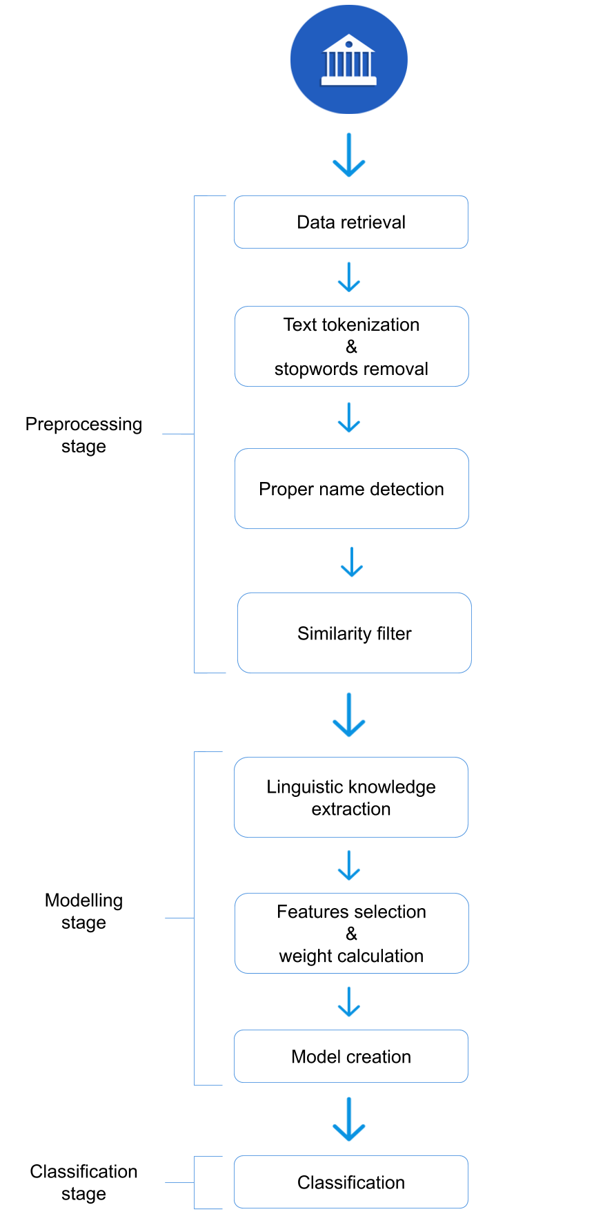
Figure 1: System stages.

III-A Preprocessing

III-A1 Data retrieval

Data was retrieved with the CoinScrap coin scrapper embedded into electronic banking apps of real users, who granted us permission. Section IV-A describes the resulting dataset.

III-A2 Text tokenization and stopwords

The language of bt descriptions is quite particular because it must be concise. The meaning of the message is condensed in few characters. In most cases verbs are totally absent. Nevertheless, bt descriptions may still contain useless information that may affect text classification.

First, each bt description is split into tokens, and, in some cases, into sentences. Then meaningless words or stopwords, such as determiners and prepositions (‘el’/‘the’, ‘en’/‘in’, ‘entonces’/‘so’, ‘aunque’/‘although’, ‘pero’/‘but’ and so on) are removed. Table I shows some stopword examples. Next, all punctuation marks apart from ‘.’ and ‘,’ are also removed.

TABLE I: Some examples of stopwords.

Stopwords
algún	como	incluso	poder	también
ambos	esta	otro	por	tras
ante	estar	para	primero	un
antes	hacer	pero	ser	uso

III-A3 Proper name detection

Finally, proper names are detected using lists of names and surnames and replaced by a tag.

Taking the real bt description ‘Compra en supermercado Elvira Madrid 28. TARJ. :*320546’ as an example, after text tokenization, stopword removal and proper name extraction, the result is ‘Compra # supermercado #PNegi# Madrid 28. TARJ. #320546’. The “#” symbol marks the place where a word is removed. Note that each proper name is substituted by “#PN” followed by a set of characters (‘egi’ in the example) and “#”. Thus, a given name is always replaced by the same identifier (‘Elvira’ by #PNegi# in the example). Credit card number was always anonymized.

III-A4 Training sample reduction with similarity detection stage

We take advantage of the fact that many bt descriptions are similar to reduce the size of the training set. For that purpose, we insert a similarity detector based on the Jaccard distance [55] before the classifier. This is inspired by spam detection techniques that use this distance to seek for characteristic sentences [56, 57, 58].

The similarity detector only considers the text of the descriptions. When the Jaccard similarity between a new labelled description and a previous entry in our dataset exceeds 85%, and both belong to the same category, the new description is not added to the svm training set. Otherwise, we keep it. When the similarity between a new unlabelled description and a previous entry exceeds 85%, we assign to the description the class of the entry. Otherwise, the description is passed to the svm for classification.

Figure 2 illustrates the architecture of the system including the Jaccard similarity detector. The svm classifier is explained in Section III-B3.

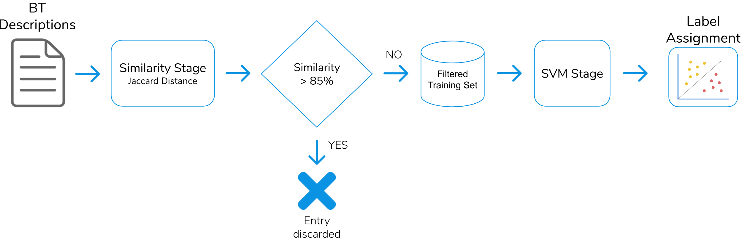
Figure 2: Flow diagram of the system with Jaccard similarity detector.

III-B Machine learning analysis

In this section we explain the knowledge-based linguistic extraction as well as the feature selection.

III-B1 Linguistic knowledge extraction

In this step we create lexica whose entries are related to the categories of the classification problem. Figure 3 represents the lexicon generation procedure.

First, starting from the preprocessed bt descriptions in the training set, which are labelled according to the classification categories, all non-alphabetic characters such as numbers, punctuation marks and symbols are cleared. Next, useful final elements for the lexica are extracted. These are the unigrams that appear at least five times in the text corpora for each category (all others are excluded) and the bigrams that are present at least three times in the corpora. Single-character alphabetic elements are also discarded. The final result is a set of lexica with unigrams and bigrams and their corresponding categories.

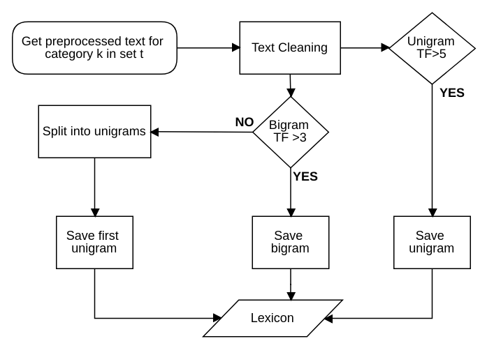
Figure 3: uml diagram of the lexicon generation procedure.

For example, let us suppose that the training set only has the following entries for a given category:

1. Compra en Pescados Diego, S.L. (‘Purchase at Pescados Diego, S.L.’)

2. Compra en supermercado Elvira Madrid 28 (‘Purchase at Elvira supermarket Madrid 28’)

3. Compra en amazon.es (‘Purchase in amazon.es’)

4. Compra en supermercado Carrefour Enero 2018 (‘Purchase at Carrefour supermarket January 2018’)

5. Compra en amazon.es Febrero 2018 (‘Purchase in amazon.es February 2018’)

6. Compra en Amazon (“Purchase in Amazon’)

7. Pago en supermercado Elvira Alicante (‘Payment at Elvira Alicante supermarket’)

8. Pago en supermercado El Corte Inglés Vigo (‘Payment at El Corte Inglés Vigo supermarket’)

9. Compra en supermercado Carrefour Febrero 2018 (‘Purchase at Carrefour supermarket February 2018’)

10. Compra en supermercado amazon.es (‘Purchase in amazon.es supermarket’)

The resulting lexicon would only contain the words ‘compra’ and ‘supermercado’ and the bigram ‘compra supermercado’ followed by the categories.

III-B2 Feature selection and weight calculation

The system uses a standard svm algorithm for modelling and prediction. Short texts are encoded according to the vector space model in [59]. The smallest data unit in the model corresponds to a feature. A text $T$ may be seen as an $n$-dimensional vector in the vector space, as follows:

$$T=((t_{1},w_{1}),(t_{2},w_{2}),...,(t_{n},w_{n}))$$ (1)

where $t$ is the value of a feature of text $T$ and $w$ its weight. The greater the $w$, the more information the feature contains in that case [60].

Many different types of features are possible, such as Boolean, word frequency (number of times a word appears in the text) and tf-idf. Note that classification results depend greatly on feature selection [61, 62]. An efficient feature selection method not only reduces the dimension of the feature space but also avoids useless features. The features in our system are the following:

1. Lexicon data. These features count the words in the bt descriptions that appear in the lexica for each existing category.

2. Amount. The range of the bt amount field, since ranges are more significant for our application than exact values. Specifically, we consider non-overlapping intervals limited by $20$, $60$, $200$, $800$, $1500$ and $3000$ euros.

3. Sign of the amount. This feature indicates if the bt is an income (positive) or an expense (negative).

4. Date. The information in the date field of each bt. Again, we use ranges. This is because some events occur on specific days of the month (e.g. salary at the end), whereas other events (e.g. purchases) may happen anytime during the month. The selected ranges were the last five, ten, twenty and twenty-five days of the month.

5. Word $n$-grams. $N$-gram representation is language-independent. It transforms documents into high-dimensional feature vectors where each feature corresponds to a contiguous sub-string. Formally, an $n$-gram consists of $n$ adjacent items from alphabet $A$. Items can be phonemes, syllables, letters, words or base pairs depending on the application. Hence, the number of different $n$-grams in a text is $|A|^{n}$ at most. The dimension of an $n$-gram feature sub-vector may therefore be very high even for moderate values of $n$. However, since not all $n$-grams are present in a document, the dimension is substantially reduced. During the formation of an $n$-gram feature sub-vector, all upper-case characters are converted into lower-case characters and punctuation marks are converted to spaces. Sub-vectors are then normalized. The optimal $n$ depends on the text corpora.

   We explain feature sub-vectors with an example that computes the $n$-grams from one to four words for the bt description ‘Operación tarjeta débito Amazon’ (‘Amazon debit card transaction’). The resulting vector consists of the following components: ‘operación’ (‘transaction’), ‘tarjeta’ (‘card’), ‘débito’ (‘debit’), amazon; ‘operación tarjeta’ (‘card transaction’), ‘tarjeta débito’ (‘debit card’), ‘débito amazon’ (‘amazon debit’); ‘operación tarjeta débito’ (‘debit card transaction’), ‘tarjeta débito amazon’ (‘amazon debit card’); ‘operación tarjeta débito amazon’ (‘amazon debit card transaction’).

6. Character $n$-grams. Character $n$-grams have been proven useful for a variety of ml problems, such as language detection. Simple models based on them have outperformed convolutional and recursive deep neural networks (cnns and rnns) [63, 64, 65].

   We illustrate them with an example that computes the trigram, four-gram and five-gram character sub-vectors for the sentence ‘Operación tarjeta débito Amazon’ (note that spaces are also taken into account when computing character $n$-grams): (ope, per, era, rac, aci, ció, ión, ón , n t, ta, tar, arj, rje, jet, eta, ta , a d, dé, déb, ébi, bit, ito, to , o a, am, ama, maz, azo, zon; oper, pera, erac, raci, ació, ción, ión , ón t, n ta, tar, tarj, arje, rjet, jeta, eta , ta d, a dé, déb, débi, ébit, bito, ito , to a, o am, ama, amaz, mazo, azon; opera, perac, eraci, ració, ación, ción , ión t, ón ta, n tar, tarj, tarje, arjet, rjeta, jeta , eta d, ta dé, a déb, débi, débit, ébito, bito , ito a, to am, o ama, amaz, amazo, mazon).

   They have been applied in scenarios with misspelling errors [66, 67]. Character $n$-grams may also capture other effects of language usage, such as re-named entities and abbreviations, e.g. ‘maths’ instead of ‘mathematics’. In our case, they are justified by the many shortened words in bt descriptions.

III-B3 svm classifier

We decompose the overall problem into pairwise two-class problems, following a one-versus-one approach. Therefore, $k(k-1)/2$ svm classification models are necessary for $k$ text classes. The category is decided by majority voting.

IV Experimental results

All experiments were performed on a computer with the following specifications:

1. Operating System: Ubuntu 18.04 LTS 64 bits

2. Processor: Intel@Core i5 3470 CPU 3.2Ghz x 4

3. RAM: 15.4 Gb

4. Disk: 1.9 Tb

IV-A Dataset

The dataset comprises 30,844 bt descriptions from customer accounts of major Spanish banks, written mostly in Spanish and issued between August 2017 and February 2018. They were collected during the CatCoin project with the collaboration of CoinScrap Finance S.L., Spain, using the CoinScrap platform. The entries of the dataset have the following attributes:

1. ID: a unique numeric identifier.

2. Description: the bt short-text description.

3. Amount: the amount in euros of the bt, either positive (income) or negative (expense).

4. Date: the date when the bt occurred.

Every entry has an extra field with the category label that determines the classification goal. The dataset may be requested to the authors by e-mail. Table II shows the numerical distributions of the fifteen categories in the dataset. Table III shows some examples of dataset entries.

TABLE II: Distribution of categories in the labelled dataset.

Category	Instances
Bank	4,835
Means of transport	3,479
Shopping	11,061
Household expenses	1,158
Taxes and charges	489
Off-cycle income	89
Payroll	248
Leisure	2,362
Health, sport and education	867
Insurances	883
Social security, grants and pensions	67
Transfers	2,086
Business and professional expenses	197
Rentals	116
Others	2,907
Total	30,844

IV-B Evaluation metrics

Due to the issues of accuracy with class asymmetries [68, 69], we employed precision, recall and $F$ metrics using a macro-average approach.

TABLE III: Examples of entries in the labelled dataset.

ID	Description	Category	Amount	Date
59da944c5858 aa32256f883a	Recibo ORANGE ESPAGNE S.A.U ‘ORANGE ESPAGNE S.A.U bill’	Household expenses	-42,29 €	Thu Sep 28 2017 02:00:00
59da944c5858 aa32256f882a	Traspaso recibido Cuenta Nómina ‘Transfer received Payroll Account’	Bank	100,00 €	Thu Oct 05 2017 02:00:00
5a046cf2d9f7 0921c74182d9	www.just-eat.es	Leisure	-39,60 €	Thu Nov 09 2017 01:00:00
5a69353d323c a817506a2bdd	RECIBO ASOC DE CONSUMIDORES EN ACCION-FACUA ‘Association of Consumers in Action-FACUA bill’	Health, sport and education	-63,00 €	Tue Jan 09 2018 01:00:00
5a8d5a8d1a33 590273326bed	TRANSFERENCIA A FAVOR DE PN CONCEPTO Alquiler Febrero 2017 + Luz ‘Transfer in favour of PN CONCEPT February 2017 rent + electricity’	Rentals	-377,75 €	Wed Feb 07 2018 01:00:00

Macro-averaged results were computed as indicated by [70]. Consider a binary evaluation metric $B(t_{p},t_{n},f_{p},f_{n})$ that is calculated based on the number of true positives ($t_{p}$), true negatives ($t_{n}$), false positives ($f_{p}$) and false negatives ($f_{n}$). Let $t_{p_{\lambda}}$, $f_{p_{\lambda}}$, $t_{n_{\lambda}}$ and $f_{n_{\lambda}}$ be the amounts of true positives, false positives, true negatives and false negatives, respectively, after binary evaluation for label $\lambda$. The macro-average evaluation metric is calculated as follows:

$$\small\displaystyle B_{macro}=\frac{1}{q}\sum_{\lambda=1}^{k}B(t_{p_{\lambda}},f_{p_{\lambda}},t_{n_{\lambda}},f_{n_{\lambda}})$$ (2)

Macro-averaging weights all classes equally, whereas micro-averaging weights all document classification decisions equally. Since $F$ ignores true negatives and its magnitude is mostly determined by the number of true positives, large classes dominate over small classes in micro-averaging [71]. For this reason we preferred the macro-average approach.

To calculate precision, recall and $F$ rates we first computed each of these measures separately for each category using expressions (3)-(5):

$$\small\displaystyle\mbox{\em Precision}_{\mbox{\footnotesize micro}_{q}}=\frac{t_{p_{q}}}{t_{p_{q}}+f_{p_{q}}}$$ (3)

$$\small\displaystyle\mbox{\em Recall}_{\mbox{\footnotesize micro}_{q}}=\frac{t_{p_{q}}}{t_{p_{q}}+f_{n_{q}}}$$ (4)

$$\small\displaystyle\mbox{\em F}_{\mbox{\footnotesize micro}_{q}}=\frac{2(\mbox{\em Precision}_{\mbox{\footnotesize micro}_{q}}*\mbox{\em Recall}_{\mbox{\footnotesize micro}_{q}})}{(\mbox{\em Precision}_{\mbox{\footnotesize micro}_{q}}+\mbox{\em Recall}_{\mbox{\footnotesize micro}_{q}})}$$ (5)

These metrics were then averaged by category using expression  (2) to produce the macro-averaged metrics.

IV-C Numerical results

We performed cross-validation in different dataset splits of training and testing subsets (in all cases the first and second percentages correspond to training and testing subset sizes, respectively): 30%-70%, 40%-60%, 60%-40% and 70%-30%. The purpose was to check the robustness of our system when fewer training data were available.

TABLE IV: Average word distribution in the lexica for the different training-testing splits before applying the similarity filter.

Lexicon	30%-70%	40%-60%	60%-40%	70%-30%
Bank	368.6	421.8	486.2	513.6
Means of transport	515	602.6	742.4	782.6
Shopping	1,551.2	1,830.2	2,295.2	2,501.4
Household expenses	191.4	226.8	280.4	307.6
Taxes and charges	101.8	128.4	159.8	169.2
Off-cycle income	13.2	18.2	24.2	113.2
Payroll	65	80.4	105	27.6
Leisure	479.6	569.8	706.4	765.2
Health, sport and education	262	310.2	393.2	437.2
Insurances	154	181.2	244.6	259.4
Social security, grants and pensions	15.2	19.2	23.4	24.2
Transfers	516.6	639.6	849.6	933
Business and professional expenses	61.8	80.4	107.8	119.6
Rentals	54.8	58.6	79.2	90
Others	160.2	190.6	226.4	241.8

In each experiment we extracted the lexica of the set as explained in Section III-B1. Table IV shows the distributions of words in the lexica for all categories before applying the similarity detector. We added features incrementally to the model to assess their significance. Therefore, first we only used word $n$-grams and lexica, then we added bt amount and date, and finally character $n$-grams features.

Given the target sector (finance), precision may be more important than recall. This is because banking campaigns prefer to obtain less positives for key categories. By doing so, they maximize the probability that customers will be receptive to personalized products.

We compared our system with three competitor approaches, All-In-1 [72] and two variants of the method by IITP (Indian Institute of Technology Patna) [73]. These approaches analyzed customer feedback to manufacturers, which also consisted of short texts, although with more elaborate sentences than bt descriptions. Note that no other researchers have considered bt to date. For the sake of fairness, we applied the Jaccard distance detector stage to the competitors as well.

The All-In-1 approach in [72] is based on a classic svm classifier that takes character $n$-grams and monolingual word embeddings as input. Logically we only used the monolingual version.

The two IITP variants [73] are based on cnns. The second variant combines a cnn with an rnn. Specifically, a convolutional feature extractor is applied to the input, a recurrent network is applied to the cnn output, an optional fully connected layer is applied to the rnn output, and finally a softmax layer delivers the result.

Tables V and VI show average elapsed training and testing times for our system and its competitors for the different splits and selections of features, obtained with cross-validation (five different dataset samplings in each experiment). For our system, the values of $n$ in character and word $n$-grams were adjusted to 3-5 and 1-4 respectively.

Note that, even though testing times were comparable, the training times of the competitors were significantly higher. This is due to their greater computational complexity. Specifically, the svm classifier of All-In-1 uses word embeddings and the two variants of IITP are based on cnns.

Table VII shows the average training set reductions that the similarity detector achieved for the different splits. Note that they exceeded 56% in all cases.

TABLE V: Elapsed training and testing times of our system for different dataset splits.

Split	Set	Instances	Features	Computing time (s)
30%-70%	Train	4,031	Word $n$-grams	2.20 $\pm$ 0.40
			Word $n$-grams + char $n$-grams	5.00 $\pm$ 1.55
			Word $n$-grams + lexica	2.20 $\pm$ 0.40
			Word $n$-grams + lexica + amount + date	2.20 $\pm$ 0.40
			Word $n$-grams + lexica + amount + date + char $n$-grams	6.20 $\pm$ 1.47
	Test	21,590	Word $n$-grams	8.20 $\pm$ 0.40
			Word $n$-grams + char $n$-grams	15.40 $\pm$ 0.49
			Word $n$-grams + lexica	10.00 $\pm$ 0.00
			Word $n$-grams + lexica + amount + date	10.40 $\pm$ 0.49
			Word $n$-grams + lexica + amount + date + char $n$-grams	18.60 $\pm$ 2.15
40%-60%	Train	4,849.40	Word $n$-grams	2.00 $\pm$ 0.00
			Word $n$-grams + char $n$-grams	5.80 $\pm$ 0.75
			Word $n$-grams + lexica	3.00 $\pm$ 0.00
			Word $n$-grams + lexica + amount + date	3.20 $\pm$ 0.40
			Word $n$-grams + lexica + amount + date + char $n$-grams	6.00 $\pm$ 0.00
	Test	18,506	Word $n$-grams	7.00 $\pm$ 0.00
			Word $n$-grams + char $n$-grams	14.00 $\pm$ 0.00
			Word $n$-grams + lexica	8.40 $\pm$ 0.49
			Word $n$-grams + lexica + amount + date	8.40 $\pm$ 0.49
			Word $n$-grams + lexica + amount + date + char $n$-grams	15.20 $\pm$ 0.40
60%-40%	Train	6,209.20	Word $n$-grams	3.00 $\pm$ 0.00
			Word $n$-grams + char $n$-grams	9.40 $\pm$ 1.50
			Word $n$-grams + lexica	4.20 $\pm$ 0.40
			Word $n$-grams + lexica + amount + date	4.00 $\pm$ 0.00
			Word $n$-grams + lexica + amount + date + char $n$-grams	9.00 $\pm$ 0.63
	Test	12,338	Word $n$-grams	5.00 $\pm$ 0.00
			Word $n$-grams + char $n$-grams	11.40 $\pm$ 0.80
			Word $n$-grams + lexica	6.20 $\pm$ 0.40
			Word $n$-grams + lexica + amount + date	6.00 $\pm$ 0.00
			Word $n$-grams + lexica + amount + date + char $n$-grams	12.00 $\pm$ 0.00
70%-30%	Train	6,780.20	Word $n$-grams	4.00 $\pm$ 0.00
			Word $n$-grams + char $n$-grams	11.20 $\pm$ 0.98
			Word $n$-grams + lexica	4.20 $\pm$ 0.40
			Word $n$-grams + lexica + amount + date	4.60 $\pm$ 0.80
			Word $n$-grams + lexica + amount + date + char $n$-grams	11.20 $\pm$ 0.40
	Test	9,253	Word $n$-grams	4.00 $\pm$ 0.00
			Word $n$-grams + char $n$-grams	9.60 $\pm$ 0.49
			Word $n$-grams + lexica	5.20 $\pm$ 0.40
			Word $n$-grams + lexica + amount + date	5.20 $\pm$ 0.40
			Word $n$-grams + lexica + amount + date + char $n$-grams	10.60 $\pm$ 0.49

TABLE VI: Elapsed training and testing times of the competitor systems for different dataset splits.

Split	Set	Instances	Features	Computing time (s)
30%-70%	Train	4,031	Word $n$-grams	2.20 $\pm$ 0.40
			Word $n$-grams + char $n$-grams	5.00 $\pm$ 1.55
			All-In-1 Word $n$-grams	1.83 $\pm$ 0.08
			All-In-1 Word $n$-grams + char $n$-grams	30.04 $\pm$ 1.66
			IITP-cnn	976.10 $\pm$ 33.34
			IITP-cnn+rnn	1153.03 $\pm$ 59.08
	Test	21,590	Word $n$-grams	8.20 $\pm$ 0.40
			Word $n$-grams + char $n$-grams	15.40 $\pm$ 0.49
			All-In-1 Word $n$-grams	1.56 $\pm$ 0.02
			All-In-1 Word $n$-grams + char $n$-grams	5.53 $\pm$ 0.16
			IITP-cnn	4.47 $\pm$ 0.37
			IITP-cnn+rnn	5.99 $\pm$ 0.62
40%-60%	Train	4,849.40	Word $n$-grams	2.00 $\pm$ 0.00
			Word $n$-grams + char $n$-grams	5.80 $\pm$ 0.75
			All-In-1 Word $n$-grams	2.28 $\pm$ 0.15
			All-In-1 Word $n$-grams + char $n$-grams	38.68 $\pm$ 1.70
			IITP-cnn	1224.89 $\pm$ 71.48
			IITP-cnn+rnn	1698.12 $\pm$ 108.46
	Test	18,506	Word $n$-grams	7.00 $\pm$ 0.00
			Word $n$-grams + char $n$-grams	14.00 $\pm$ 0.00
			All-In-1 Word $n$-grams	1.33 $\pm$ 0.04
			All-In-1 Word $n$-grams + char $n$-grams	5.01 $\pm$ 0.12
			IITP-cnn	3.85 $\pm$ 0.28
			IITP-cnn+rnn	5.80 $\pm$ 0.19
60%-40%	Train	6,209.20	Word $n$-grams	3.00 $\pm$ 0.00
			Word $n$-grams + char $n$-grams	9.40 $\pm$ 1.50
			All-In-1 Word $n$-grams	2.93 $\pm$ 0.08
			All-In-1 Word $n$-grams + char $n$-grams	61.95 $\pm$ 3.68
			IITP-cnn	2025.20 $\pm$ 22.99
			IITP-cnn+rnn	2759.47 $\pm$ 66.43
	Test	12,338	Word $n$-grams	5.00 $\pm$ 0.00
			Word $n$-grams + char $n$-grams	11.40 $\pm$ 0.80
			All-In-1 Word $n$-grams	0.91 $\pm$ 0.02
			All-In-1 Word $n$-grams + char $n$-grams	3.91 $\pm$ 0.16
			IITP-cnn	2.90 $\pm$ 0.09
			IITP-cnn+rnn	4.45 $\pm$ 0.13
70%-30%	Train	6,780.20	Word $n$-grams	4.00 $\pm$ 0.00
			Word $n$-grams + char $n$-grams	11.20 $\pm$ 0.98
			All-In-1 Word $n$-grams	3.21 $\pm$ 0.09
			All-In-1 Word $n$-grams + char $n$-grams	69.35 $\pm$ 1.75
			IITP-cnn	2327.73 $\pm$ 38.76
			IITP-cnn+rnn	3072.74 $\pm$ 327.81
	Test	9,253	Word $n$-grams	4.00 $\pm$ 0.00
			Word $n$-grams + char $n$-grams	9.60 $\pm$ 0.49
			All-In-1 Word $n$-grams	0.69 $\pm$ 0.02
			All-In-1 Word $n$-grams + char $n$-grams	3.30 $\pm$ 0.10
			IITP-cnn	2.37 $\pm$ 0.06
			IITP-cnn+rnn	3.41 $\pm$ 0.12

TABLE VII: Training sample reduction for different dataset splits.

Split	Instances	Instances after similarity detection
30%-70%	9,254	4,031
40%-60%	12,338	4,849
60%-40%	18,506	6,209
70%-30%	21,591	6,780

IV-C1 30%-70% split

In each experiment the training dataset had in average 4,031 entries (after similarity detection) and the testing dataset had 21,590 entries.

Tables VIII and IX show the results of bt classification. Note that we did not modify the design or the implementation of the selected competitors. Thus, for a fair comparison, only word and character $n$-grams features were enabled in Table VIII. Our system outperformed the competitors in terms of precision and All-In-1 was the best option in recall and $F$-measure.

TABLE VIII: Average evaluation metrics for the basic combinations of features, 30%-70% split.

Train	Test	Features	$\mbox{P}_{\mbox{\tiny\bf macro}}$	$\mbox{R}_{\mbox{\tiny\bf macro}}$	$\mbox{F}_{\mbox{\tiny\bf macro}}$
30%	70%	Proposed system word $n$-grams	68.19%	25.70%	37.32%
		Proposed system word $n$-grams + char $n$-grams	93.36%	76.30%	83.97%
		All-In-1 word $n$-grams	90.87%	85.22%	87.67%
		All-In-1 word $n$-grams + char $n$-grams	90.75%	86.87%	88.57%
		IITP-cnn	87.83%	81.02%	83.78%
		IITP-cnn+rnn	88.27%	75.05%	80.32%

In Table IX we observe that, after activating the lexicon feature, the precision, recall and $F$ of our system increased by about 15%, 38% and 35%, respectively, so the lexicon feature was crucial. Another key result is that meta-information features yielded a precision increase of 8% in our system. After activating all features, precision, recall and $F$ further improved by around 3%, 19% and 13%, respectively.

TABLE IX: Average evaluation metrics of the proposed system for all combinations of features, 30%-70% split.

Train	Test	Features	$\mbox{P}_{\mbox{\tiny\bf macro}}$	$\mbox{R}_{\mbox{\tiny\bf macro}}$	$\mbox{F}_{\mbox{\tiny\bf macro}}$
30%	70%	Word $n$-grams	68.19%	25.70%	37.32%
		Word $n$-grams + lexica	82.90%	63.51%	71.90%
		Word $n$-grams + lexica + amount + date	91.31%	64.92%	75.87%
		Word $n$-grams + lexica + amount + date + char $n$-grams	94.59%	84.15%	89.06%

Our system attained the best precision, but only attained better $F$ than All-In-1 if all features are activated. On the other hand, All-In-1 was better in recall but the difference with our system in that regard was only about 3%. Note, however, that regardless of the fact that precision is more important in our scenario, our system is simpler than its competitors (based, depending on the case, on cnn, cnn+rnn or a svm with word embeddings), especially in terms of training time, as shown in tables V and VI.

IV-C2 40%-60% split

In this case, in each experiment the training dataset had in average 4,849 annotated entries (after similarity detection) and the testing dataset had 18,506 entries.

Tables X and XI show the results. In this case our improvement in precision with the basic features was about 2% compared to the competitors. The precision, recall and $F$ of our system increased by about 17%, 37% and 34%, respectively, after activating the lexica feature. By adding meta-information, the improvements were 7%, 3% and 5%, respectively. Total precision, recall and $F$ improved compared to the baseline (word $n$-grams) by about 2%, 18% and 12%, respectively, after activating all the features.

TABLE X: Average evaluation metrics for the basic combinations of features, 40%-60% split.

Train	Test	Features	$\mbox{P}_{\mbox{\tiny\bf macro}}$	$\mbox{R}_{\mbox{\tiny\bf macro}}$	$\mbox{F}_{\mbox{\tiny\bf macro}}$
40%	60%	Proposed system word $n$-grams	68.25%	27.36%	39.05%
		Proposed system word $n$-grams + char $n$-grams	93.56%	78.72%	85.50%
		All-In-1 word $n$-grams	91.69%	87.12%	89.05%
		All-In-1 word $n$-grams + char $n$-grams	90.99%	88.11%	89.27%
		IITP-cnn	90.27%	84.06%	86.70%
		IITP-cnn+rnn	88.84%	77.93%	82.15%

TABLE XI: Average evaluation metrics of the proposed system for all combinations of features, 40%-60% split.

Train	Test	Features	$\mbox{P}_{\mbox{\tiny\bf macro}}$	$\mbox{R}_{\mbox{\tiny\bf macro}}$	$\mbox{F}_{\mbox{\tiny\bf macro}}$
40%	60%	Word $n$-grams	68.25%	27.36%	39.05%
		Word $n$-grams + lexica	85.54%	64.50%	73.53%
		Word $n$-grams + lexica + amount + date	92.94%	67.30%	78.05%
		Word $n$-grams + lexica + amount + date + char $n$-grams	95.43%	85.43%	90.15%

We again attained the best precision performance, outperforming the best competitor by almost 4% when all features are activated.

IV-C3 60%-40% split

The training dataset had in average 6,209 annotated entries (after similarity detection) and the testing dataset was composed of 12,338 entries.

Tables XII and XIII summarize the results. Table XII shows that our system had the best precision performance if both word and character $n$-grams features are enabled, but All-In-1 was still the best alternative in terms of recall and $F$ for the basic combinations of features. In this case, the precision, recall and $F$ metrics of our system improved versus the baseline by about 27%, 58% and 50%, respectively, after activating all the features. We again attained the best precision, outperforming the best competitor by almost 2% when all features are activated. Our system ranked second in recall after All-In-1 by a narrow margin of about 3% again when all features are activated. We remark again that we are not using semantic information from word embeddings.

TABLE XII: Average evaluation metrics for the basic combinations of features, 60%-40% split.

Train	Test	Features	$\mbox{P}_{\mbox{\tiny\bf macro}}$	$\mbox{R}_{\mbox{\tiny\bf macro}}$	$\mbox{F}_{\mbox{\tiny\bf macro}}$
60%	40%	Proposed system word $n$-grams	68.54%	29.24%	40.97%
		Proposed system word $n$-grams + char $n$-grams	94.38%	80.42%	86.83%
		All-In-1 word $n$-grams	92.74%	89.75%	91.12%
		All-In-1 word $n$-grams + char $n$-grams	90.98%	89.89%	90.29%
		IITP-cnn	90.54%	85.15%	87.37%
		IITP-cnn+rnn	89.97%	81.42%	85.02%

TABLE XIII: Average evaluation metrics of the proposed system for all combinations of features, 60%-40% split.

Train	Test	Features	$\mbox{P}_{\mbox{\tiny\bf macro}}$	$\mbox{R}_{\mbox{\tiny\bf macro}}$	$\mbox{F}_{\mbox{\tiny\bf macro}}$
60%	40%	Word $n$-grams	68.54%	29.24%	40.97%
		Word $n$-grams + lexica	85.74%	65.42%	74.21%
		Word $n$-grams + lexica + amount + date	93.14%	68.28%	78.79%
		Word $n$-grams + lexica + amount + date + char $n$-grams	95.60%	87.05%	91.12%

IV-C4 70%-30% split

The training dataset had in average 6,780 annotated entries (after similarity detection) and the testing dataset had 9,253 entries.

Tables XIV and XV show the results. With the basic features all systems achieved similar results (Table XIV). In this case, the precision, recall and $F$ of our system improved by about 28%, 57% and 49%, respectively after activating all the features. We again attained the best precision and almost matched All-In-1 in terms of recall and $F$ when all features are activated.

TABLE XIV: Average evaluation metrics for the basic combinations of features, 70%-30% split.

Train	Test	Features	$\mbox{P}_{\mbox{\tiny\bf macro}}$	$\mbox{R}_{\mbox{\tiny\bf macro}}$	$\mbox{F}_{\mbox{\tiny\bf macro}}$
70%	30%	Proposed system word $n$-grams	67.41%	30.67%	42.16%
		Proposed system word $n$-grams + char $n$-grams	94.37%	80.15%	86.88%
		All-In-1 word $n$-grams	92.58%	90.01%	91.16%
		All-In-1 word $n$-grams + char $n$-grams	91.35%	89.95%	90.52%
		IITP-cnn	89.33%	85.67%	87.19%
		IITP-cnn+rnn	90.06%	82.14%	85.63%

TABLE XV: Average evaluation metrics of the proposed system for all combinations of features, 70%-30% split.

Train	Test	Features	$\mbox{P}_{\mbox{\tiny\bf macro}}$	$\mbox{R}_{\mbox{\tiny\bf macro}}$	$\mbox{F}_{\mbox{\tiny\bf macro}}$
70%	30%	Word $n$-grams	67.41%	30.67%	42.16%
		Word $n$-grams + lexica	87.91%	66.71%	75.84%
		Word $n$-grams + lexica + amount + date	92.99%	70.22%	80.01%
		Word $n$-grams + lexica + amount + date + char $n$-grams	95.05%	87.51%	91.12%

Table XVI shows the performance of our system by bt category when all the features are enabled. In general the performance was satisfactory. The worst performance corresponded to the categories with fewer entries in the training set (according to Table II).

TABLE XVI: Performance of our system by category with all features enabled, 70%-30% split.

Category	$\mbox{P}_{\mbox{\tiny\bf macro}}$	$\mbox{R}_{\mbox{\tiny\bf macro}}$	$\mbox{F}_{\mbox{\tiny\bf macro}}$
Bank	92.32%	93.08%	92.69%
Means of transport	94.54%	90.06%	92.24%
Shopping	89.88%	98.07%	93.79%
Household expenses	98.15%	91.35%	94.62%
Taxes and charges	96.34%	82.18%	88.58%
Off-cycle income	95.32%	88.89%	91.97%
Payroll	95.92%	88.11%	91.76%
Leisure	95.24%	87.36%	91.12%
Health, sport and education	97.01%	82.38%	89.10%
Insurances	98.29%	94.87%	96.54%
Social security, grants and pensions	98.89%	85.00%	91.31%
Transfers	88.84%	80.19%	84.29%
Business and professional expenses	89.12%	73.22%	80.31%
Rentals	98.00%	82.86%	89.77%
Others	97.85%	95.02%	96.42%

IV-D Summary of numerical results

To evaluate the performance of our system we applied cross-validation in five dataset splits between training and testing subsets (30%-70%, 40%-60%, 60%-40% and 70%-30%), to check the robustness of our approach as the sizes of the testing subsets decreased. In these experiments we added features to the model incrementally to assess their significance, in the following order: word $n$-grams, lexica, amount, date and character $n$-grams. We compared our system with three competing approaches from the state-of-the-art, All-In-1 and two variants of the IITP method.

The Jaccard similarity detector achieved reductions of training data exceeding 56% for all splits.

For the 30%-70% split, our system attained the best precision. It was inferior to All-In-1 in recall and $F$ unless all features were enabled. If they were, our system also outperformed its competitors in $F$. For the 40%-60% split, our system outperformed the competitors in terms of precision, recall and $F$ when all features were enabled. It was better in precision even with the basic combination of features. For the 60%-40% and 70%-30% splits, our system again outperformed the competitors in terms of precision, and the performance gap with All-In-1, in the cases it existed, was reduced. Indeed, our approach is simpler than the competitors, which allowed significant training time reduction.

V Use case:CoinScrap

CoinScrap launched its mobile app for iOS and Android in November 2016, and since then it has had thousands of downloads. A new version of the application was launched October 2018. It includes journey improvement for product fulfilment; dynamic “gamified” saving rules (e.g. saving when your favourite team wins, or when you take a coffee); and personalised recommendations for financial management.

The latter rely on our system to classify bt transactions. In this line, CoinScrap recommends personalized services and products based on financial necessities and objectives. Figure 4 shows an screenshot of the app.

Figure 4: Coinscrap app.

VI Conclusions

Compared to normal texts, short texts analysis is challenging due to sparsity, irregularity and real-time data generation. In this paper we describe a short-text svm bt classification system using a combination of meta-information and linguistic knowledge (by relying on specialized lexica).

Motivated by existing solutions in spam detection, we achieved a significant reduction of training information with a short text similarity detector based on the Jaccard distance.

Experimental results, by comparing our approach with three state-of-the-art competitors with higher computational complexity, are very promising. Our lexicon feature is crucial to attain high precision, especially if the training dataset is small.

The effectiveness of the proposed system was demonstrated on a real dataset reflecting the activity of real customers of Spanish banks, organized in fifteen different classes including means of transport, shopping, household expenses, taxes, charges and payroll. This labelled dataset is a valuable asset that will be available to other researchers on request.

Our system attained the best precision (which is the most relevant metric in pfm) and performed similarly in terms of recall and $F$ if enough features were enabled, especially when the methods were stressed by reducing the training-to-test subset size ratio.

Given the encouraging results in this work, we are currently expanding it to obtain sub-categorisations of the descriptions. Our approach has been put into production in a real pfm application, CoinScrap.

References

- [1] B. L. Derby, “Data mining for improper payments,” The Journal of Government Financial Management, vol. 52, no. 4, p. 10, 2003.
- [2] E. W. Ngai, L. Xiu, and D. C. Chau, “Application of data mining techniques in customer relationship management: A literature review and classification,” Expert Systems With Applications, vol. 36, no. 2, pp. 2592–2602, 2009.
- [3] X. Hu, “A data mining approach for retailing bank customer attrition analysis,” Applied Intelligence, vol. 22, no. 1, pp. 47–60, 2005.
- [4] M. R. Islam and M. A. Habib, “A Data Mining Approach to Predict Prospective Business Sectors for Lending in Retail Banking Using Decision Tree,” International Journal of Data Mining & Knowledge Management Process, vol. 5, no. 2, pp. 13–22, 2015.
- [5] C. Chekuri, M. H. Goldwasser, P. Raghavan, and E. Upfal, “Web search using automatic classification,” in Proceedings of the Sixth International Conference on the World Wide Web, 1997, pp. 1–10.
- [6] D.-T. Vo and Y. Zhang, “Target-Dependent Twitter Sentiment Classification with Rich Automatic Features.” in Proc. IJCAI, 2015, pp. 1347–1353.
- [7] G. Kumaran and J. Allan, “Text classification and named entities for new event detection,” in Proceedings of the 27th Annual International ACM SIGIR Conference on Research and Development in Information Retrieval. ACM, 2004, pp. 297–304.
- [8] Y. Cai, W.-H. Chen, H.-F. Leung, Q. Li, H. Xie, R. Y. Lau, H. Min, and F. L. Wang, “Context-aware ontologies generation with basic level concepts from collaborative tags,” Neurocomputing, vol. 208, pp. 25–38, 2016.
- [9] Q. Du, H. Xie, Y. Cai, H.-F. Leung, Q. Li, H. Min, and F. L. Wang, “Folksonomy-based personalized search by hybrid user profiles in multiple levels,” Neurocomputing, vol. 204, pp. 142–152, 2016.
- [10] Y. LeCun, Y. Bengio, and G. Hinton, “Deep learning,” Nature, vol. 521, no. 7553, p. 436, 2015.
- [11] A. M. Hormozi and S. Giles, “Data mining: A competitive weapon for banking and retail industries,” Information Systems Management, 2004.
- [12] O. Aregbeyen, “The determinants of bank selection choices by customers: Recent and extensive evidence from Nigeria,” International Journal of Business and Social Science, vol. 2, no. 2, pp. 276–288, 2011.
- [13] H. U. Rehmann and S. Ahmed, “An empirical analysis of the determinants of bank selection in Pakistan: A customer view,” Pakistan Economic and Social Review, vol. 46, no. 2, pp. 147–160, 2008.
- [14] V. Dinh and L. Pickler, “Examining service quality and customer satisfaction in the retail banking sector in Vietnam,” Journal of Relationship Marketing, vol. 11, no. 4, pp. 199–214, 2012.
- [15] A. Keramati, H. Ghaneei, and S. M. Mirmohammadi, “Developing a prediction model for customer churn from electronic banking services using data mining,” Financial Innovation, vol. 2, no. 1, p. 10, dec 2016.
- [16] A. Sharma and P. Kumar Panigrahi, “A Neural Network based Approach for Predicting Customer Churn in Cellular Network Services,” International Journal of Computer Applications, vol. 27, no. 11, pp. 26–31, 2011.
- [17] K. Chen, Y.-H. Hu, and Y.-C. Hsieh, “Predicting customer churn from valuable B2B customers in the logistics industry: A case study,” Inf. Syst. E-bus. Manag., vol. 13, no. 3, pp. 475–494, 2015.
- [18] S. Barman, U. Pal, M. A. Sarfaraj, B. Biswas, A. Mahata, and P. Mandal, “A complete literature review on financial fraud detection applying data mining techniques,” International Journal of Trust Management in Computing and Communications, vol. 3, no. 4, pp. 336–359, 2016.
- [19] J. West and M. Bhattacharya, “Intelligent financial fraud detection: A comprehensive review,” Computers & Security, vol. 57, pp. 47 – 66, 2016.
- [20] Y. Yoshimura, A. Amini, S. Sobolevsky, J. Blat, and C. Ratti, “Analysis of customers’ spatial distribution through transaction datasets,” in Transactions on Large-Scale Data and Knowledge-Centered Systems XXVII - Volume 9860. New York, NY, USA: Springer-Verlag New York, Inc., 2016, pp. 177–189.
- [21] R. Vahidov and X. He, “Situated DSS for personal finance management: Design and evaluation,” Information & Management, vol. 47, no. 2, pp. 78–86, 2010.
- [22] D. A. Zetzsche, D. W. Arner, R. P. Buckley, and R. H. Weber, “The Future of Data-Driven Finance and RegTech: Lessons from EU Big Bang II,” University of New South Wales Law Research Series, Australasian Legal Information Institute Level 14, 61 Broadway, Australia, Tech. Rep. [2019] UNSWLRS 22, 2019.
- [23] M. F. Caropreso, S. Matwin, and F. Sebastiani, “A learner-independent evaluation of the usefulness of statistical phrases for automated text categorization,” Text Databases and Document Management: Theory and Practice, vol. 5478, pp. 78–102, 2001.
- [24] P. S. Jacobs, “Joining statistics with NLP for text categorization,” in Proceedings of the Third Conference on Applied Natural Language Processing. Association for Computational Linguistics, 1992, pp. 178–185.
- [25] H. Lodhi, C. Saunders, J. Shawe-Taylor, N. Cristianini, and C. Watkins, “Text classification using string kernels,” Journal of Machine Learning Research, vol. 2, no. Feb, pp. 419–444, 2002.
- [26] L. D. Baker and A. K. McCallum, “Distributional clustering of words for text classification,” in Proceedings of the 21st Annual International ACM SIGIR Conference on Research and Development in Information Retrieval. ACM, 1998, pp. 96–103.
- [27] Z. S. Harris, “Distributional structure,” Word, vol. 10, no. 2-3, pp. 146–162, 1954.
- [28] A. McCallum, K. Nigam et al., “A comparison of event models for naive bayes text classification,” in Proc. AAAI-98 Workshop on Learning for Text Categorization, vol. 752, 1998, pp. 41–48.
- [29] K. Nigam, J. Lafferty, and A. McCallum, “Using maximum entropy for text classification,” in Proc. IJCAI-99 Workshop on Machine Learning for Information Filtering, vol. 1, 1999, pp. 61–67.
- [30] T. Joachims, “Text categorization with support vector machines: Learning with many relevant features,” in European Conference on Machine Learning. Germany: Springer, 1998, pp. 137–142.
- [31] F. Sebastiani, “Machine learning in automated text categorization,” ACM Computing Surveys (CSUR), vol. 34, no. 1, pp. 1–47, 2002.
- [32] D. D. Lewis, “An evaluation of phrasal and clustered representations on a text categorization task,” in Proceedings of the 15th Annual International ACM SIGIR Conference on Research and Development in Information Retrieval. ACM, 1992, pp. 37–50.
- [33] M. Post and S. Bergsma, “Explicit and implicit syntactic features for text classification,” in Proceedings of the 51st Annual Meeting of the Association for Computational Linguistics, vol. 2, 2013, pp. 866–872.
- [34] T. Nakagawa, K. Inui, and S. Kurohashi, “Dependency tree-based sentiment classification using CRFs with hidden variables,” in Human Language Technologies: The 2010 Annual Conference of the North American Chapter of the Association for Computational Linguistics. Association for Computational Linguistics, 2010, pp. 786–794.
- [35] M. Karo and P. Stephen, “Sentiment composition,” in Proc. of Recent Advances in Natural Language Processing (RANLP), 2007, pp. 378–382.
- [36] S. Wang and C. D. Manning, “Baselines and bigrams: Simple, good sentiment and topic classification,” in Proceedings of the 50th Annual Meeting of the Association for Computational Linguistics: Short Papers-Volume 2. Association for Computational Linguistics, 2012, pp. 90–94.
- [37] Y. Bengio, R. Ducharme, P. Vincent, and C. Jauvin, “A neural probabilistic language model,” Journal of Machine Learning Research, vol. 3, pp. 1137–1155, 2003.
- [38] R. Collobert, J. Weston, L. Bottou, M. Karlen, K. Kavukcuoglu, and P. Kuksa, “Natural language processing (almost) from scratch,” Journal of Machine Learning Research, vol. 12, pp. 2493–2537, 2011.
- [39] T. Mikolov, K. Chen, G. Corrado, and J. Dean, “Efficient estimation of word representations in vector space,” arXiv preprint arXiv:1301.3781, 2013.
- [40] R. Socher, J. Pennington, E. H. Huang, A. Y. Ng, and C. D. Manning, “Semi-supervised recursive autoencoders for predicting sentiment distributions,” in Proceedings of the Conference on Empirical Methods in Natural Language Processing. Association for Computational Linguistics, 2011, pp. 151–161.
- [41] N. Kalchbrenner, E. Grefenstette, and P. Blunsom, “A convolutional neural network for modelling sentences,” arXiv preprint arXiv:1404.2188, 2014.
- [42] C. dos Santos and M. Gatti, “Deep convolutional neural networks for sentiment analysis of short texts,” in Proceedings of COLING 2014, the 25th International Conference on Computational Linguistics: Technical Papers, 2014, pp. 69–78.
- [43] Q. Le and T. Mikolov, “Distributed representations of sentences and documents,” in Proc. International Conference on Machine Learning, 2014, pp. 1188–1196.
- [44] C. C. Aggarwal and C. Zhai, “A Survey of Text Clustering Algorithms,” in Mining Text Data. Boston: Springer, 2012, pp. 77–128.
- [45] S. Banerjee, K. Ramanathan, and A. Gupta, “Clustering short texts using Wikipedia,” in Proceedings of the 30th Annual International ACM SIGIR Conference on Research and Development in Information Retrieval. ACM, 2007, pp. 787–788.
- [46] S. Fodeh, B. Punch, and P.-N. Tan, “On ontology-driven document clustering using core semantic features,” Knowledge and Information Systems, vol. 28, no. 2, pp. 395–421, 2011.
- [47] J. Yin and J. Wang, “A Dirichlet multinomial mixture model-based approach for short text clustering,” in Proceedings of the 20th ACM SIGKDD International Conference on Knowledge Discovery and Data Mining. ACM, 2014, pp. 233–242.
- [48] D. Cai, X. He, and J. Han, “Document clustering using locality preserving indexing,” IEEE Transactions on Knowledge and Data Engineering, vol. 17, no. 12, pp. 1624–1637, 2005.
- [49] S. Lai, L. Xu, K. Liu, and J. Zhao, “Recurrent Convolutional Neural Networks for Text Classification.” in Proc. AAAI, vol. 333, 2015, pp. 2267–2273.
- [50] W. Wu, H. Li, H. Wang, and K. Q. Zhu, “Probase: A probabilistic taxonomy for text understanding,” in Proceedings of the 2012 ACM SIGMOD International Conference on Management of Data. ACM, 2012, pp. 481–492.
- [51] E. Gabrilovich and S. Markovitch, “Computing semantic relatedness using Wikipedia-based explicit semantic analysis,” in Proc. IJCAI, vol. 7, 2007, pp. 1606–1611.
- [52] X. Han and J. Zhao, “Named entity disambiguation by leveraging Wikipedia semantic knowledge,” in Proceedings of the 18th ACM conference on Information and knowledge management. ACM, 2009, pp. 215–224.
- [53] X. Hu, X. Zhang, C. Lu, E. K. Park, and X. Zhou, “Exploiting Wikipedia as external knowledge for document clustering,” in Proceedings of the 15th ACM SIGKDD International Conference on Knowledge Discovery and Data Mining. ACM, 2009, pp. 389–396.
- [54] X. Ni, J.-T. Sun, J. Hu, and Z. Chen, “Mining multilingual topics from Wikipedia,” in Proceedings of the 18th International Conference on World Wide Web. ACM, 2009, pp. 1155–1156.
- [55] C. Seung-Seok, C. Sung-Hyuk, and C. C. Tappert, “A Survey of Binary Similarity and Distance Measures,” Journal of Systemics, Cybernetics & Informatics, vol. 8, no. 1, pp. 43–48, 2010.
- [56] S. R. Harsule and M. K. Nighot, “N-Gram Classifier System to Filter Spam Messages from OSN User Wall,” in Advances in Intelligent Systems and Computing. Singapore: Springer, 2016, pp. 21–28.
- [57] S. Bajaj, N. Garg, and S. K. Singh, “A Novel User-based Spam Review Detection,” Procedia Computer Science, vol. 122, pp. 1009–1015, 2017.
- [58] S. Temma, M. Sugii, and H. Matsuno, “The Document Similarity Index based on the Jaccard Distance for Mail Filtering,” in Proceedings of the 34th International Technical Conference on Circuits/Systems, Computers and Communications. IEEE, 2019, pp. 1–4.
- [59] C. Yin, “Towards Accurate Node-Based Detection of P2P Botnets,” The Scientific World Journal, pp. 1–10, 2014.
- [60] C. Yin, M. Zou, D. Iko, and J. Wang, “Botnet detection based on correlation of malicious behaviors,” Int J Hybrid Inf Technol, vol. 6, no. 6, pp. 291–300, 2013.
- [61] A. Veeraswamy and D. S. A. Balamurugan, “A Survey of Feature Selection Algorithms in Data Mining,” in Proceedings of the 3rd International Conference on Trends in Information Sciences and Computing (TISC-2011), 2011, pp. 40–46.
- [62] X.-J. Tong, M.-G. Cui, and G.-L. Song, “Research on Chinese Text Automatic Categorization Based on VSM,” in Proc. International Conference on Wireless Communications, Networking and Mobile Computing. IEEE, 2007, pp. 3863–3866.
- [63] M. Medvedeva, M. Kroon, and B. Plank, “When sparse traditional models outperform dense neural networks: the curious case of discriminating between similar languages,” in VarDial, 2017, pp. 156–163.
- [64] S. Malmasi, K. Evanini, A. Cahill, J. Tetreault, R. Pugh, C. Hamill, D. Napolitano, and Y. Qian, “A report on the 2017 native language identification shared task,” in Proceedings of the 12th Workshop on Innovative Use of NLP for Building Educational Applications. Association for Computational Linguistics, 2017, pp. 62–75.
- [65] A. Kulmizev, B. Blankers, J. Bjerva, M. Nissim, G. van Noord, B. Plank, and M. Wieling, “The power of character n-grams in native language identification,” in BEA@EMNLP. Association for Computational Linguistics, 2017, pp. 382–389.
- [66] W. Cavnar, “Using an n-gram-based document representation with a vector processing retrieval model,” NIST Special Publication, pp. 269–269, 1995.
- [67] S. Huffman, “Acquaintance: Language-independent document categorization by n-grams,” Department of Defense Ft. George G. Meade, 4409 Llewellyn Ave, Fort Meade, MD 20755, United States, Tech. Rep. 0704-0188, 1995.
- [68] M. Sokolova and G. Lapalme, “A systematic analysis of performance measures for classification tasks,” Inf. Process. Manage., vol. 45, no. 4, pp. 427–437, Jul. 2009.
- [69] R. G. Rossi, A. d. A. Lopes, and S. O. Rezende, “Optimization and label propagation in bipartite heterogeneous networks to improve transductive classification of texts,” Inf. Process. Manage., vol. 52, no. 2, pp. 217–257, Mar. 2016.
- [70] G. Tsoumakas, I. Katakis, and I. Vlahavas, “Mining multi-label data,” in Data Mining and Knowledge Discovery Handbook. Boston: Springer, 2009, pp. 667–685.
- [71] C. D. Manning, P. Raghavan, H. Schütze et al., Introduction to Information Retrieval. Cambridge University Press, Cambridge, 2008, vol. 1.
- [72] B. Plank, “All-in-1: Short text classification with one model for all languages,” in Proceedings of the International Joint Conference on Natural Language Processing (Shared Task 4). Association for Computational Linguistics, December 2017.
- [73] D. Gupta, P. Lenka, H. Bedi, A. Ekbal, and P. Bhattacharyya, “IITP at IJCNLP-2017 task 4: Auto analysis of customer feedback using CNN and GRU network,” in Proceedings of the IJCNLP 2017, Shared Tasks. Asian Federation of Natural Language Processing, 2017, pp. 184–193.