Functional reducibility of higher-order networks

Abstract

Empirical complex systems are widely assumed to be characterized not only by pairwise interactions, but also by higher-order (group) interactions that affect collective phenomena, from metabolic reactions to epidemics. Nevertheless, higher-order networks’ superior descriptive power—compared to classical pairwise networks—comes with a much increased model complexity and computational cost. Consequently, it is of paramount importance to establish a quantitative method to determine when such a modeling framework is advantageous with respect to pairwise models, and to which extent it provides a parsimonious description of empirical systems. Here, we propose a principled method, based on information compression, to analyze the reducibility of higher-order networks to lower-order interactions, by identifying redundancies in diffusion processes while preserving the relevant functional information. The analysis of a broad spectrum of empirical systems shows that, although some networks contain non-compressible group interactions, others can be effectively approximated by lower-order interactions—some technological and biological systems even just by pairwise interactions. More generally, our findings mark a significant step towards minimizing the dimensionality of models for complex systems.

Introduction

Many complex systems exhibit an interconnected structure that can be encoded by pairwise interactions between their constituents. Such pairwise interactions have been used to model biological, social and technological systems, providing a powerful descriptive and predictive framework [1, 2, 3, 4, 5, 6]. Recently, the analysis of higher-order structural patterns and dynamical behaviors attracted the attention of the research community as a powerful framework to model group interactions [7, 8, 9, 10], with applications ranging from neuroscience [11, 12] to ecology [13] and social sciences [14, 15], highlighting the emergence of novel phenomena and non-trivial collective behavior [16, 17, 18, 19, 20, 21].

Higher-order networks encode more information than pairwise interactions: for example, metabolic reactions are more realistically described by group interactions between any number of reagents and reactants, capturing information that would be lost by considering the union of pairwise interactions instead. However, this modeling flexibility comes at a cost: new data needs to be adequately recorded and stored as group interactions instead of pairwise ones, and new analytical [22, 23, 24, 25] and computational [26, 27, 28] tools need to be developed. Moreover, the complexity and computational cost of these tools increase exponentially as larger group interactions are considered.

It is therefore crucial to understand under which conditions higher-order representations need to be favored over classical pairwise ones, and whether it is possible to devise a grounded procedure to determine which representation provides the most parsimonious description of an empirical system.

A similar challenge was faced nearly a decade ago, when the advent of temporal and categorical data [29, 30, 31] allowed multilayer representations of complex networks [32]. For these representations, a principled approach was used to show that not all layers, or types of interaction, are equally informative: Some information can be discarded or aggregated to reduce the overall complexity of the model without sacrificing its descriptive power [33, 34]. Although multilayer networks are different from higher-order networks, this approach, formally based on the density matrix formalism [35], provides a good candidate for the present case. Indeed, the idea is similar to the widely used information compression algorithms adopted in computer science: by exploiting the regularities in the data, one can build a compressed representation that optimizes the number of bits needed to describe the data with a model and those to encode the model itself. Similar approaches have also been used to coarse-grain complex and multiplex networks [36, 37, 38].

Here, we build on this long-standing research line and propose a principled approach to optimally compress systems with higher-order interactions—accounting for the complexity of the data and the complexity of the model. Specifically, we determine an optimal order of interactions up to which interactions need be considered to obtain a functionally optimal representation of the system—larger orders can be safely discarded. Formally, we do so by generalizing the concept of network density matrix [35, 39] to account for higher-order diffusive dynamics with the multiorder Laplacian [40, 17] and calculate a message length corresponding to each order. By minimizing this message length, in the spirit of the original minimum message length principle [41], we find the optimal compression of the data which, in turn, corresponds to the most parsimonious functional description of the system. In the following, we refer to this procedure as functional reduction. A higher-order network is fully reducible—to a pairwise network—if the optimal order is 1, while its reducibility decreases for increasing optimal orders. We demonstrate the validity of our method by performing an extensive analysis of synthetic networks and investigate the functional reducibility of a broad spectrum of real-world higher-order systems.

The advantage of this framework is that it provides a bridge between network analysis and information theory by means of a formalism that is largely inspired by quantum statistical physics, which has found a variety of applications from systems biology [42] to neuroscience [43], shedding light on fundamental mechanisms such as the emergence of network sparsity [44] and the renormalization group [45].

Results

.1 Density matrix for higher-order networks

The flow of information between nodes in a (pairwise) network can be modeled by different dynamical processes. Arguably, the simplest and most successful of these processes is diffusion, that can be described by means of the propagator $e^{-\tau\mathbf{L}}$, where $\mathbf{L}$ the combinatorial Laplacian and $\tau$ is the diffusion time. In particular, the information flow from node $i$ to node $j$ is described by the component $\left(e^{-\tau\mathbf{L}}\right)_{ij}$. Network states can then be encoded by a density matrix [35, 39] defined as

$$\bm{\rho}_{\tau}=\frac{e^{-\tau\mathbf{L}}}{Z},$$ (1)

where the partition function $Z=\text{Tr}\left(e^{-\tau\mathbf{L}}\right)$ ensures a unit trace for this operator.

Figure 1: Functional reducibility of higher-order networks. Illustration of our method with an example hypergraph. Given (a) an original hypergraph with interactions of orders up to $d_{\rm max}$ ($=3$, here), (b) we compute the message length, a trade-off between information loss and model complexity, of the same hypergraph, but considering orders only up to $d$. We determine the optimal order $d_{\rm opt}$ as that that minimizes the message length. Finally, (c) we reduce the original hypergraph to an optimal version by considering orders up to $d_{\rm opt}$.

Here, we generalize density matrices to higher-order networks. The most general formalism to encode higher-order networks is that of hypergraphs [8]. A hypergraph is defined by a set of nodes and a set of hyperedges that represent the interactions between any number of those nodes. A hyperedge is said to be of order $d$ if it involves $d+1$ nodes: a 0-hyperedge is a node, a 1-hyperedge is a 2-node interaction, a 2-hyperedge is a 3-node interaction, and so on. Simplicial complexes are a special case of hypergraph that is also commonly used: they additionally require that each subset of each hyperedge is included, too. In a hypergraph $H$ with maximum order $d_{\rm max}$, diffusion between nodes through hyperedges of order up to $D\leq d_{\rm max}$ can be described by the multiorder Laplacian [40, 46]

$$\mathbf{L}^{[D]}\equiv\mathbf{L}^{(D,\text{ mul})}=\sum_{d=1}^{D}\frac{\gamma_{d}}{\langle K^{(d)}\rangle}\mathbf{L}^{(d)},$$ (2)

which is a weighted sum of the Laplacians $\mathbf{L}^{(d)}$ at each order $d$ up to order $D$ . At each order, the weight is defined by a real coefficient $\gamma_{d}$ (which we set to 1 for simplicity) and the averaged generalized degrees $\left<K^{(d)}\right>$. Each $d$-order Laplacian is defined by $L^{(d)}_{ij}=K^{(d)}_{i}\delta_{ij}-\frac{1}{d}A^{(d)}_{ij}$, in terms of the generalized degrees $\bm{K}^{(d)}$ and adjacency matrix $\mathbf{A}^{(d)}$ of order $d$. The matrix $\mathbf{L}^{[D]}$ satisfies all the properties expected from a Laplacian: it is positive semidefinite and its rows (columns) sum to zero (see Methods for details).

Accordingly, the multiorder density matrix of hypergraph $H$, up to order $d$, is defined as

$$\bm{\rho}^{[d]}_{\tau}=\frac{e^{-\tau\mathbf{L}^{[d]}}}{Z},$$ (3)

with the partition function $Z=\text{Tr}\left(e^{-\tau\mathbf{L}^{[d]}}\right)$. Just like its pairwise analog in Eq. 1, this operator satisfies all the expected properties of a density matrix: it is positive definite and its eigenvalues sum up to one. Importantly, the diffusion time $\tau$ plays the role of a topological scale parameter: small values of $\tau$ allow information to diffuse only to neighboring nodes, probing only short-scale structures. Larger values of $\tau$, instead, allow the diffusion to reach more remote parts of the hypergraph and describe large-scale structures. In this context, the meaning of “small” and “large” depends on the network structure, and can be estimated with respect to the magnitude of the largest ($1/\lambda_{\max}$) and smallest ($1/\lambda_{\min}$) eigenvalues of the Laplacians, respectively.

.2 Quantifying the reducibility of a hypergraph

We approach the reducibility of a hypergraph as a problem of model selection. We formulate that problem as follows: given a hypergraph $H$ with maximum order $d_{\rm max}$, is $H$ an optimal representation of itself, or is considering only its hyperedges up to a given order $d<d_{\rm max}$ sufficient? Formally, we treat the density matrix $\bm{\rho}^{[d_{\rm max}]}$ as data and $\bm{\rho}^{[d]}$ as a model of the data. Formulated in this way, we need to find the “optimal” model of the data, that is, to evaluate the optimal order $d_{\rm opt}$. To define “optimal”, we use the minimum message length formalism: the model needs to represent the data as accurately as possible while remaining as simple as possible, akin to Occam’s Razor. The steps of the methods are illustrated in Fig. 1: (a) start from an original hypergraph, (b) calculate the optimal largest order $d_{\rm opt}$ by minimizing the message length, and (c) reduce the original hypergraph to an optimal hypergraph, that is, one with orders only up to $d_{\rm opt}$ without losing functional information.

As illustrated in Fig. 2, we define the message length $\mathcal{L}$ as the sum of the information loss – the opposite of the model accuracy – of the model, measured by a suitably generalized Kullback-Leibler divergence $D_{\rm KL}$, and the model complexity $C$ (see Methods for details):

$$\mathcal{L}\left(\bm{\rho}_{\tau}^{[d_{\rm max}]}|\bm{\rho}_{\tau}^{[d]}\right)=D_{\rm KL}\left(\bm{\rho}_{\tau}^{[d_{\rm max}]}|\bm{\rho}_{\tau}^{[d]}\right)+C\left(\bm{\rho}_{\tau}^{[d]}\right).$$ (4)

Note that by definition, there is no information loss when considering all possible orders, i.e., $D_{\rm KL}\left(\bm{\rho}_{\tau}^{[d_{\rm max}]}|\bm{\rho}_{\tau}^{[d_{\rm max}]}\right)=0$. Accordingly, the optimal order $d_{\rm opt}$ is that that minimizes the message length:

$$d_{\rm opt}=\operatorname*{arg\,min}\limits_{d}\mathcal{L}\left(\bm{\rho}_{\tau}^{[d_{\rm max}]}|\bm{\rho}_{\tau}^{[d]}\right).$$ (5)

Finally, we define the reducibility of the hypergraph as

$$\chi(H)=\frac{d_{\rm max}-d_{\rm opt}}{d_{\rm max}-1},$$ (6)

which measures the ratio between the number of orders to reduce and the maximum number of orders to reduce, $d_{\rm max}-1$. By construction, $\chi(H)=0$ for a hypergraph that is not reducible at all, i.e., $d_{\rm opt}=d_{\rm max}$, while $\chi(H)=1$ for a hypergraph that is maximally reducible, that is, it can be optimally reduced to its pairwise interactions, $d_{\rm opt}=1$.

.3 Rescaling the diffusion time $\tau$ at each order

As mentioned above, a topological scale $\tau$ may be large for some networks but low for others, which is a challenge when the aim is to compare networks. To overcome this problem, we rescale $\tau$ to ensure an appropriate diffusion time for each structure, and we exploit examples of hypergraphs with certain regularities to define a baseline and characterize the scaling relation.

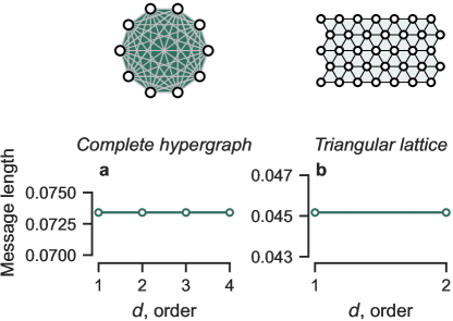
Specifically, there is a class of hypergraphs for which Laplacians of different orders are proportional, i.e., $\mathbf{L}^{(d)}\propto\mathbf{L}^{(d^{\prime})}$. This occurs in very regular structures including complete hypergraphs and some simplicial complex lattices (see Methods). In this case, since the Laplacian matrices govern the flow of information, all orders and all their combinations encode the same functional information. Consequently, we expect to see these structures to be functionally invariant under reduction—i.e., the message length should not change as one reduces the hypergraph.

However, without rescaling, the summation of Laplacian matrices according to Eq. 2 simply strengthens the flow pathways in the original hypergraph, making it different from its reduced versions. To correct for this effect, we rescale $\tau$ to allow meaningful comparisons between hypergraphs of different orders.

Since the density matrix only depends on the product of $\tau\mathbf{L}^{(d)}$, this can be achieved by selecting a value of diffusion time $\tau$, and then rescaling it to obtain a new $\tau^{\prime}(d)$ at each order like so:

$$\tau^{\prime}(d)=\frac{d_{\rm max}}{d}\tau.$$ (7)

This ensures that the multiorder density matrices are all equal

$$\bm{\rho}_{\tau^{\prime}(d)}^{[d]}=\bm{\rho}_{\tau}^{[d_{\rm max]}}\quad\forall d,$$ (8)

in the special case of hypergraphs with proportional Laplacian matrices, and gives a flat message length in those extreme structures (Fig. S1).

For illustration purposes, we set $\tau=1/\lambda_{N}$ in numerical experiments, unless otherwise stated, where $\lambda_{N}$ is the largest eigenvalue of the multiorder Laplacian of the original hypergraph $\mathbf{L}^{[d_{\rm max}]}$.

Physically, this rescaling simply means that we adapt the topological scale at which we probe the hypergraph as we consider more orders, to highlight the distribution of flow pathways rather than their accumulated strengths. We use this rescaling of $\tau$ at each order, in all hypergraphs (see Methods for details). In other words, we compute the message length $\mathcal{L}\left(\bm{\rho}_{\tau}^{[d_{\rm max}]}|\bm{\rho}_{\tau^{\prime}(d)}^{[d]}\right)$ where the $\tau$ of the reduced hypergraph is rescaled, contrary to Eq. 4.

.4 Random structures

We now investigate the reducibility of two types of heterogeneous random structures: random hypergraphs and random simplicial complexes. To do so, we compute the optimal order as described above.

A random hypergraph is defined by a number of nodes $N$ and a set of wiring probability $p_{d}$ for each order required. At each order $d$, a hyperdedge is created for any combination of $d+1$ nodes with probability $p_{d}$, similarly to Erdős-Rényi networks. Random simplicial complexes are built in the same manner before adding the missing subfaces of all simplices, to respect the condition of inclusion. In both cases, we set $N=100$, $p_{d}=50/N^{d}$ and $d_{\rm max}=4$.

Figure 2: Message length is the sum of information loss and model complexity. Example curve for a random simplicial complex. The minimum message length is indicated by the vertical line. Parameters were set to $N=100$ nodes and wiring probabilities $p_{d}=50/N^{d}$ at order $d$ with $d_{\rm max}=4$.

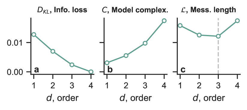
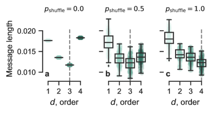
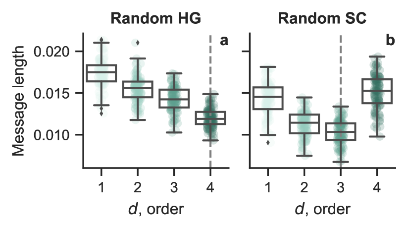
Figure 3 shows the message length considering orders from 1 to 4, for 100 realizations of each type of random structure. In random hypergaphs (Fig. 3a), the optimal order is the maximum, $d_{\rm opt}=4=d_{\rm max}$. This means that those random hypergraphs, at this diffusion scale $\tau=1/\lambda_{N}$, are not reducible, i.e., $\chi=0$. Instead, in the random simplicial complex case, $d_{\rm opt}=3$, reflecting a higher reducibility $\chi=1/3$.

The only difference between these two cases is that the hyperedges between different orders are correlated (nested) in random simplicial complexes but not in random hypergraphs. To test the effect of this feature, we start from random simplicial complexes and gradually change them to random hypergraphs by shuffling their hyperedges. Specifically, we change each hyperedge into another inexisting hyperedge with probability $p_{\rm shuffle}$. For $p_{\rm shuffle}=1$, the result is a random hypergraph, and Fig. S2 shows the results that confirm the above pattern.

Figure 3: Reducibility of random higher-order networks. (a) Random hypergraphs and (b) random simplicial complexes, 100 realizations for each. The minimum message length is indicated by the vertical line. Parameters were set to $N=100$ nodes and wiring probabilities $p_{d}=50/N^{d}$ at order $d$ with $d_{\rm max}=4$.

.4.1 Effect of the diffusion time $\tau$ and density

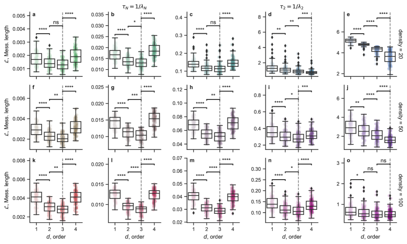
As mentioned above, $\tau$ acts as a topological scale. Diffusion processes with different values of $\tau$ are thus expected to “see” different structures, which may result in different optimal order and reduced hypergraph. To illustrate this, we compute the message length curves for the random simplicial complex case, for five values of $\tau$ evenly spaced on a logarithmic scale, and where the second and fourth are $1/\lambda_{N}$ and $1/\lambda_{2}$, respectively. Figure S3 shows that as the topological scale increases (larger $\tau$), the message length (i) increases overall and (ii) the reducibility decreases to $\chi=0$. Figure S5 shows the same results for three values of the hyperedge density, where we can see that for higher densities, the message length curve becomes much more flat with no clear minimum (see Figure S5), suggesting a functional similarity between the large-scale structure at all orders.

We similarly tested the effect of the sole density on the reducibility (Figs. S4 and S5). In general, the overall density coefficient does not seem to significantly affect the reducibility.

.5 Real-world hypergraphs

We now investigate how reducible real-world hypergraphs are by considering 22 empirical hypergraph datasets from 4 categories: coauthorships, face-to-face contacts, biological systems, and online communications (“technological”).

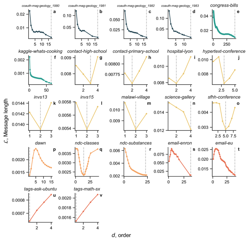
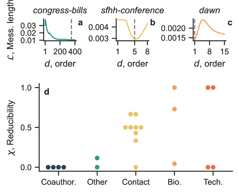
First, we observe a great variety in the reducilibity values (Fig. 4) and the associated message length curves (Fig. S6). Fig. 4a-c show three examples with curves of very different shapes and with different reduciblity. Second, we note that datasets from different categories seem to be distinctively reducible: all coauthorship datasets are not reducible ($\chi=0$), half of the technological datasets are fully reducible (tag datasets, $\chi=1$) and the other half is not (email datasets, $\chi=0$), whereas most contact datasets have medium values of reducibility. The number of nodes, the maximum and optimal orders, and the hypergraph reducibility are reported for all datasets in Table 1, and a description of the datasets is provided in Methods.

In Fig. S7, we also show the reducibility values against structural parameters of the hypergraphs: number of nodes, number of edges, density, and maximum order. We did not observe clear correlations with any of those parameters. In particular, the reducibility takes many values between 0 and 1 for any value of the structural parameters, which confirms the variety of reducibility values in the empirical datasets.

Figure 4: Empirical datasets show different levels of reducibility. We show the message length again the largest order considered in (a) congress-bills, (b) sfhh-conference, and (c) dawn. (a) Reducibility $\chi$ for datasets by category. All reducibility values are reported in Table 1.

Dataset	Category	$N$	$d_{\rm max}$	$d_{\rm opt}$	$\chi$
coauth-mag-geology_1980	coauthorship	1350	17	17	0.00
coauth-mag-geology_1981	coauthorship	464	17	17	0.00
coauth-mag-geology_1982	coauthorship	1331	17	17	0.00
coauth-mag-geology_1983	coauthorship	535	14	14	0.00
congress-bills	other	1718	399	353	0.12
kaggle-whats-cooking	other	6714	64	64	0.00
contact-high-school	contact	327	4	3	0.33
contact-primary-school	contact	242	4	2	0.67
hospital-lyon	contact	75	4	2	0.67
hypertext-conference	contact	113	5	3	0.50
invs13	contact	92	3	2	0.50
invs15	contact	217	3	2	0.50
science-gallery	contact	410	4	4	0.00
sfhh-conference	contact	403	8	5	0.43
malawi-village	contact	84	3	2	0.50
dawn	bio	2290	15	1	1.00
ndc-classes	bio	628	38	11	0.73
ndc-substances	bio	3065	24	23	0.04
email-enron	technology	143	36	36	0.00
email-eu	technology	986	39	39	0.00
tags-ask-ubuntu	technology	3021	4	1	1.00
tags-math-sx	technology	1627	4	1	1.00

Table 1: Reducibility of real-world higher-order networks. We report the number of nodes $N$, the maximum order $d_{\rm max}$, the optimal order $d_{\rm opt}$, the reducibility $\chi$, and the category of a range of higher-order networks from empirical datasets. The reducibility values are shown for each category in Fig. 4.

Discussion

All areas of natural and social science, as well as engineering ones, are undergoing a deluge of publicly available data with complex structure. This data allows for building more detailed and powerful models of systems from areas such as physics, biology, sociology, and technology. One class of such models is networks that encode group interactions rather than just pairwise ones: higher-order networks. Higher-order networks provide a natural framework for modeling systems where interactions between more than two units occur, such as chemical reactions of metabolic interest or social interactions. However, they are usually projected—by design—to pairwise interactions when data is gathered, and higher-order information is inevitably lost. By preserving that information, higher-order networks have the potential to yield a more reliable model of some empirical systems. Nevertheless, higher-order networks with novel challenges: new theoretical and computational methods have to be developed, while algorithms become exponentially more complex for increasing order of the interactions. It is thus of paramount importance to understand under which conditions one should opt for higher-order modeling—or keep using traditional pairwise models.

Here, we have provided a principled method, at the edge between statistical physics and information theory, to guide researchers in identifying the most suitable representation for their data. Our method is based on minimizing a suitable message length, encoding both the number of bits required to describe the data given a model and the number of bits required to describe the model, to find the optimal order of group interactions. Orders above the optimal one can be safely discarded because they provide only redundant information about the system while increasing model complexity and the computational cost for its analysis.

Remarkably, we show that not all systems require a higher-order model to be described and that even within the same class of systems, there is some level of variability. We started by testing the method on extremely regular cases, where the message length was flat for all orders, as computed analytically. We then applied the method to random structures, where results indicate that random hypergraphs are non-reducible: i.e., they are best represented by considering all possible orders of interaction. This result is expected because random hypergraphs are the most uncorrelated model possible: hyperedges are uncorrelated within each order, just like in Erdős-Rényi random graphs, but hyperedges of different orders are also uncorrelated, yielding incompressibility of the representation. In other words, all orders are relevant to describe the system’s structure and dynamics, since they encode genuine uncorrelated noise that is incompressible. Conversely, random simplicial complexes were reducible because hyperedges at different orders are correlated by design: the presence of correlation introduces some level of redundancy that is captured by our method.

Finally, we applied our method to empirical datasets that contain group interactions. The large variety of reducibility values obtained indicates that while the extra information encoded in higher-order networks may be optimal for some systems, others can be optimally represented with lower orders and in some cases even with only pairwise interactions. It is also important to note that the category of systems to which the datasets belong appears to be correlated with its reducibility, although more datasets are needed to perform a systematic and quantitative analysis of this phenomenon. Our results challenge the widespread assumption that complex network data must necessarily be investigated through the lens of higher-order dynamics. In fact, there are completely reducible and non-reducible systems, with a complete spectrum of cases between these two extremal cases, demonstrating that some orders might be irrelevant or uninformative to describe an empirical system. In the next future, for instance, it will be important to gather novel datasets from biological sciences to test if, and in which cases, complex networks such as metabolomes and connectomes are either reducible or irreducible, to understand under which conditions higher-order mechanisms and behaviors are essential for the function of those systems as largely assumed nowadays.

The detection of redundancies, together with a principled approach to exploit the presence of regularities to identify a compressed representation of the data, has the potential to enhance our understanding of empirical higher-order systems, and contributes to the increasing interest in dimensionality reduction of such networks [48, 49, 50]. The main advantage of our framework is that it builds on a consolidated formalism that is firmly grounded on the statistical physics of strongly correlated systems. As in the case of multilayer systems [33], we think that it is remarkable that it is possible to tackle such challenges by capitalizing on a formal analogy between quantum and higher-order systems, which can be further exploited to gain novel insights about the structural and functional organization of complex systems.

Methods

.6 Multiorder Laplacian for hypergraphs

The Laplacian matrix $\mathbf{L}$ of a graph is defined as $L_{ij}=K_{i}\delta_{ij}-A_{ij}$, where $K_{i}$ is the degree of node $i$, $\delta_{ij}$ is the Kronecker delta, and $\mathbf{A}$ is the adjacency matrix. For hypergraphs, we can define $d_{\mathrm{max}}$ Laplacian matrices, one for each order of interaction. The Laplacian of order $d$ can be defined as [40, 17]

$$L^{(d)}_{ij}=K^{(d)}_{i}\delta_{ij}-\frac{1}{d}A^{(d)}_{ij},$$ (9)

where $K^{(d)}_{i}$ is the degree of order $d$ of node $i$, i.e., the number of $d$-hyperedges connected to node $i$, while $\mathbf{A}^{(d)}$ is the adjacency matrix of order $d$, whose elements $A^{(d)}_{ij}$ counts the number of $d$-hyperedges connected to nodes $i$ and $j$.

We can hence define the multiorder Laplacian up to an order $D$ as [40, 17]

$$\mathbf{L}^{[D]}=\mathbf{L}^{(D,\mathrm{mul})}=\sum\limits_{d=1}^{D}\frac{\gamma_{d}}{\langle k^{(d)}\rangle}\mathbf{L}^{(d)},$$ (10)

where $\gamma_{d}$ is a tuning parameter of interactions of order $d$, while $\langle K^{(d)}\rangle$ is the average degree of order $d$. For simplicity, in this study, we always set $\gamma_{d}=1$.

Note that in general, a hypergraph does not need to have hyperedges at every order below $D$, unless it is a simplicial complex. If there is no hyperedge of order $d$, both the Laplacian and the average degree in Eq. 2 vanish and the result is undefined. In those cases, the sum thus needs to be taken over all orders below $D$ that exist: $\mathcal{D}=\{d\leq D:\langle K^{(d)}\rangle>0\}$.

.7 Information loss as Kullback-Leibler divergence between two hypergraphs

The state of the original hypergraph $H$ is stored in the multiorder density matrix

$$\bm{\rho}_{\tau}^{[d_{\rm max}]}=e^{-\tau\mathbf{L}^{[d_{\rm max}]}}/Z^{[d_{\rm max}]},$$ (11)

and the state of the a reduced hypergraph where we consider orders up to $d$ is given by

$$\bm{\rho}_{\tau}^{[d]}=e^{-\tau\mathbf{L}^{[d]}}/Z^{[d]}.$$ (12)

To perform model selection and determine the optimal order $d_{\rm opt}$ to represent the hypergraph, we treat $\bm{\rho}_{\tau}^{[d_{\rm max}]}$ as data and $\bm{\rho}_{\tau}^{[d]}$ as a model of it. The first key aspect of a good model is that it must describe the data as accurately as possible. We can quantity the modeling error, or information loss, with the Kullback-Leibler (KL) entropy divergence between the data and the model, defined as

$$D_{\rm KL}\left(\bm{\rho}_{\tau}^{[d_{\rm max}]}|\bm{\rho}_{\tau}^{[d]}\right)=-S^{[d_{\rm max}]}+S\left([d_{\rm max}]|[d]\right)\geq 0,$$ (13)

where $S^{[d_{\rm max}]}=-\text{Tr}\left(\bm{\rho}_{\tau}^{[d_{\rm max}]}\log{\bm{\rho}_{\tau}^{[d_{\rm max}]}}\right)$ is the Von Neumann entropy of the hypergraph and $S([d_{\rm max}]|[d])=-\text{Tr}\left(\bm{\rho}_{\tau}^{[d_{\rm max}]}\log{\bm{\rho}_{\tau}^{[d]}}\right)$ is the cross-entropy between the hypergraph and its reduced form.

The Von Neumann entropy of a hypergraph can also be written as

$$S^{[d]}=-\text{Tr}\left(\bm{\rho}_{\tau}^{[d]}\log{\bm{\rho}_{\tau}^{[d]}}\right)=\sum_{i}\lambda_{i}\log\lambda_{i},$$ (14)

where $\{\lambda_{i}\}$ are the eigenvalues of the density matrix. The Von Neumann entropy $S^{[d]}$ is zero if only one eigenvalue is non-zero (“pure state”, in the language of quantum mechanics), and maximal equal to $\log N$ if all eigenvalues are equal (“maximally mixed state”, in the language of quantum mechanics). This occurs when all eigenvalues are zero: $N$ isolated nodes.

The information loss $D_{\rm KL}$ takes positive values proportionally to the inaccuracy of the mode, and reaches zero at $d=d_{\rm max}$—as the data is the most accurate model of itself.

.8 Model complexity

Accuracy, or in contrast, information loss, is insufficient to determine the optimal model and thus the order $d$. In fact, a model can always be made more accurate by overfitting. Thus, high model accuracy must be balanced with low model complexity.

We measure the complexity of the model in terms of its entropic deviation from the simplest possible model: a network of isolated nodes. We know that the entropy of $N$ isolated nodes is given by $S_{\rm iso}=\log{N}$. This gives an upper bound on the Von Neumann entropy of a hypergraph, guaranteeing that $S^{[d]}\leq S_{\rm iso}$. Therefore, we define the model complexity $C$ as:

$$C\left(\bm{\rho}_{\tau}^{[d]}\right)=S_{\rm iso}-S^{[d]}.$$ (15)

By definition, the model complexity is non-negative, $C\geq 0$, and is expected to be lower when the eigenvalues of $\bm{\rho}_{\tau}^{[d]}$ are all similar, and larger when they are more diverse.

.9 Minimizing the message length

We can now define the message length $\mathcal{L}$ by combining the information loss in Eq. 13 and the model complexity in Eq. 15:

$$\mathcal{L}\left(\bm{\rho}_{\tau}^{[d_{\rm max}]}|\bm{\rho}_{\tau}^{[d]}\right)=D_{\rm KL}\left(\bm{\rho}_{\tau}^{[d_{\rm max}]}|\bm{\rho}_{\tau}^{[d]}\right)+C\left(\bm{\rho}_{\tau}^{[d]}\right).$$ (16)

By definition, minimizing the message length corresponds to maximizing the accuracy of the model and, at the same time, minimizing the model complexity (Occam’s Razor). To obtain the best compression, we find the smallest order $d$ which gives

$$d_{\rm opt}=\min\limits_{d}\mathcal{L}\left(\bm{\rho}_{\tau}^{[d_{\rm max}]}|\bm{\rho}_{\tau}^{[d]}\right).$$ (17)

It is worth mentioning that the propagation scale $\tau$ works as a resolution parameter. When $\tau$ is very large, the process approaches the steady state, and the network topology becomes irrelevant and, consequently, any model can be a good model. Whereas, at very small $\tau$, the field evolution is linear and through the paths of length $\approx 1$, exhibiting maximum resolution. Although we explore a variety of values of $\tau$, we mainly focus on a characteristic propagation scale $\tau_{c}$, the largest $\tau$ for which a linearization of the time evolution operator is still valid. Assume the eigenvalues of the Laplacian are given by $\{\lambda_{\ell}\}$ where $\ell=1,2,...N$ and let $\lambda_{N}$ be the largest of them. Then, the eigenvalues of the time-evolution operator $e^{-\tau\mathbf{L}}$ are given by $\{e^{-\tau\lambda_{\ell}}\}$. Here, $\tau_{c}=1/\lambda_{N}$, ensuring that the last eigenvalue of the time evolution operator is reasonably linearizable $e^{-\tau_{c}\lambda_{N}}\approx 1-\tau_{c}\lambda{N}$. This ensures an acceptable linearization for the rest of the eigenvalues since $\lambda_{N}$ is the largest eigenvalue of the Laplacian.

.10 Rescaling $\tau$

.10.1 Complete hypergraph

In some extremely regular structures, such as complete hypergraphs or some simplicial complex lattices, the Laplacians at all orders are proportional. For example, for complete hypergraphs,

$$\mathbf{L}^{(d)}=\frac{K^{(d)}}{N-1}\mathbf{L}^{(1)},$$ (18)

and consequently

$$\mathbf{L}^{[d]}=\frac{d}{N-1}\mathbf{L}^{(1)}=d\,\mathbf{L}^{[1]}.$$ (19)

Another direct but useful consequence of this is the relationship between the multiorder Laplacians at any two orders

$$\mathbf{L}^{[d]}=\frac{d}{d^{\prime}}\,\mathbf{L}^{[d^{\prime}]}.$$ (20)

Since by definition Eq. 3, the density matrix $\bm{\rho}_{\tau}^{[d]}$ depends only on the product $\tau\mathbf{L}^{[d]}$, we can write

$$\bm{\rho}^{[d]}_{\tau}=\frac{e^{-\tau d\,\mathbf{L}^{[1]}}}{\text{Tr}\left(e^{-\tau d\,\mathbf{L}^{[1]}}\right)}=\bm{\rho}^{[1]}_{\tilde{\tau}}$$ (21)

where $\tilde{\tau}=d\tau$, or equivalently, between two orders

$$\bm{\rho}_{\tau}^{[d]}=\bm{\rho}_{\frac{d}{d^{\prime}}\tau}^{[d^{\prime}]}.$$ (22)

Hence, instead of selecting a single diffusion time $\tau$ for all orders, we can select a different, more appropriate diffusion time at each order. Specifically, we can select a main $\tau$, and rescale it at each order to ensure that the density matrices are the same. One could choose the rescaling so that the density matrices would be equal to any of them non-rescaled, e.g. to $\bm{\rho}_{\tau}^{[1]}$. However, to ensure that the information loss vanishes when considering all possible orders, $D_{\rm KL}\left(\bm{\rho}_{\tau}^{[d_{\rm max}]}|\bm{\rho}_{\tau}^{[d_{\rm max}]}\right)=0$, we need to set all of them equal to $\bm{\rho}_{\tau}^{[1]}$. This is achieved by rescaling the diffusion time by

$$\tau^{\prime}(d)=\frac{d_{\rm max}}{d}\tau$$ (23)

so that

$$\bm{\rho}_{\tau^{\prime}(d)}^{[d]}=\bm{\rho}_{\frac{d_{\rm max}}{d}\tau}^{[d]},=\bm{\rho}_{\tau}^{[d_{\rm max]}}.$$ (24)

.10.2 General case of proportional Laplacians

In general, the Laplacian of order $d$ is proportional to that of order $1$, $\mathbf{L}^{(d)}\propto\mathbf{L}^{(1)}$, when their respective adjacency matrices are proportional, that is

$$\mathbf{A}^{(d)}=d\,B(d)\mathbf{A}^{(1)}.$$ (25)

where $B(d)$ is a coefficient that may depend on the order $d$. Indeed, by definition, the generalized degree and adjacency matrix are related by $K_{i}^{(d)}=\frac{1}{d}\sum_{j}A^{(d)}_{ij}$, and thus we also have

$$\bm{K}^{(d)}=B(d)\bm{K}^{(1)},$$ (26)

ensuring that the Laplacian matrices are proportional, $\mathbf{L}^{(d)}=B(d)\mathbf{L}^{(1)}$.

Equation 26 implies that

$$B(d)=\langle K^{(d)}\rangle/\langle K^{(1)}\rangle,$$ (27)

and hence, the multiorder Laplacian up to order $d$ is given by

$$\mathbf{L}^{[d]}=\frac{d}{\langle K^{(1)}\rangle}\mathbf{L}^{(1)}=d\,\mathbf{L}^{[1]}$$ (28)

which is consistent with the complete hypergraph case in Eq. 18, where we have $\langle K^{(1)}\rangle=N-1$. The rest of the derivation is thus the same as in the complete graph case: rescaling $\tau$ per order as

$$\tau^{\prime}(d)=\frac{d_{\rm max}}{d}\tau$$ (29)

ensures

$$\bm{\rho}_{\tau^{\prime}(d)}^{[d]}=\bm{\rho}_{\frac{d_{\rm max}}{d}\tau}^{[d]},=\bm{\rho}_{\tau}^{[d_{\rm max]}}.$$ (30)

Note again that, in general, a hypergraph does not need to have hyperedges at every order below $D$, unless it is a simplicial complex. If there is no hyperedge at some orders $d$, Eq. 28 must be adjusted, as the factor $d$ comes from the number of orders present. The set of orders present is in general $\mathcal{D}=\{i\leq d:\langle K^{(i)}\rangle>0\}$, so that Eq. 28 becomes $\mathbf{L}^{[d]}=|\mathcal{D}|\,\mathbf{L}^{[1]}$ and Eq. 29 becomes $\tau^{\prime}(d)=\frac{d_{\rm max}}{|\mathcal{D}|}\tau$.

.10.3 Higher-order lattices

For a triangular lattice in which every triangle is promoted to a $2$-simplex, each node is part of six $1$-simplices and six $2$-simplices. Furthermore, each $1$-simplex of the lattice is part of two different $2$-simplices. This means that each pair of nodes share two 2-simplices if they share one 1-simplex, and zero otherwise. Formally:

$$k^{(2)}_{i}=6=k^{(1)}_{i}\quad\mathrm{and}\quad A^{(2)}_{ij}=2A^{(1)}_{ij},$$ (31)

so that $B(2)=1$.

.11 Description of the datasets

We assigned a category to each of the 22 empirical datasets. All datasets are accessible via XGI [26] and stored at https://zenodo.org/communities/xgi/.

Each of the coauthorship datasets corresponds to papers published in a single year (1980, 1981, 1982, 1983). A node represents an author, and a hyperedge represents a publication marked with the “Geology” tag in the Microsoft Academic Graph [51].

In the contact datasets, a node represents a person and a hyperedge represents a group or people in close proximity at a given time. Most of the original datasets are from the SocioPatterns collaboration [52, 53].

The biological datasets include two constructed in [24] with data from the National Drug Code Directory (NDC). In ndc-classes, a node represents a label (a short text description of a drug’s function) and a hyperedge represents a set of those labels applied to a given drug. In ndc-substances, a node represents a substance and a hyperedege is the set of substances in a given drug. The Drug Abuse Warning Network (DAWN) is a national health surveillance system that records drug use that contributes to hospital emergency department visits throughout the United States. A node represents a drug, and a hyperedge is the set of drugs used by a given patient (as reported by the patient) in an emergency department visit. For a period of time, the recording system only recorded the first 16 drugs reported by a patient, so the dataset only uses the first 16 drugs (at most).

The technological datasets include two email datasets and two tag ones. In the email datasets, a node represents an email address and a hyperedge is the set of all recipient addresses included in an email, including the sender’s. In the tags datasets, a node represents a tag, and a hyperedge is a set of tags associated to a question on online Stack Exchange forums (Mathematics Stack Exchange and Ask Ubuntu). The tag datasets were constructed in [24] with data from the Stack Exchange data dump.

The other datasets contain two datasets. In congress-bills, constructed in [24], a node represents a member of the US Congress and a hyperedge is the set of members co-sponsoring a bill between 1973-2016. In kaggle-whats-cooking [54], a node represents a food ingredient and a hyperedge is the set of ingredients used in a given recipe.

Data availability: All data is publically available from XGI-data: https://zenodo.org/communities/xgi/about.

Code availability: Code for reproducing our results is available online from the repository https://github.com/maximelucas/hypergraph_reducibility. It uses the XGI package [26].

Figure S1: Hypergraphs with proportional Laplacians at each order have a flat message length. (a) Complete hypergraph, (b) triangular lattice flag complex. Parameters were set to $10$ and $35$ nodes, respectively with $d_{\rm max}=4$ and 2, respectively.

Figure S2: Effect of nestedness on reducibility. We show the message length, as a function of the order, of (a) a single random simplicial complex, and then after randomly shuffling (b) 50%, and (c) all of its hyperedges, corresponding to a random hypergraph. From left to right, the nestedness between hyperedges of different orders decreases, and each point corresponds to one of 100 shuffling realizations. The minimum message length is indicated by the vertical dashed grey line. Parameters were set to $N=100$ nodes and wiring probabilities $p_{d}=50/N^{d}$ at order $d$ with $d_{\rm max}=4$.

Figure S3: Effect of $\tau$. We show the message length for a random simplicial complex, as a function of order $d$, for increasing values of the base diffusion time $\tau$ (from left to right). The second and fourth values are $\tau_{N}=1/\lambda_{N}$ and $\tau_{2}=1/\lambda_{2}$ based on eigenvalues of the multiorder density matrix. Other values are chosen to be evenly spaced in logarithmic scale. The minimum message length is indicated by the vertical line. Parameters were set to $N=100$ nodes and wiring probabilities $p_{d}=50/N^{d}$ at order $d$ with $d_{\rm max}=4$. Stars indicate a statistically significant different between two distributions ($t$-test, $s$ stars indicate $p<10^{-s}$).

Figure S4: Effect of density. We show the message length for a random simplicial complex, as a function of order $d$, for increasing values of the density coefficient (from left to right), i.e., wiring probabilities are $p_{d}=20/N^{d}$, $p_{d}=50/N^{d}$, and $p_{d}=100/N^{d}$ at order $d$. The minimum message length is indicated by the vertical line. Parameters were set to $N=100$ nodes and $d_{\rm max}=4$, with $\tau=1/\lambda_{N}$. Stars indicate a statistically significant different between two distributions ($t$-test, $s$ stars indicate $p<10^{-s}$).

Figure S5: Effect of density and diffusion time. We show the message length for a random simplicial complex, as a function of order $d$, for increasing values of the base diffusion time $\tau$ (from left to right) and density (from top to bottom). The second and fourth values of diffusion time are $\tau_{N}=1/\lambda_{N}$ and $\tau_{2}=1/\lambda_{2}$ based on eigenvalues of the multiorder density matrix. Other values are chosen to be evenly spaced in logarithmic scale. The minimum message length is indicated by the vertical line. Parameters were set to $N=100$ nodes and wiring probabilities are $p_{d}=20/N^{d}$, $p_{d}=50/N^{d}$, and $p_{d}=100/N^{d}$ at order $d$. with $d_{\rm max}=4$. Stars indicate a statistically significant different between two distributions ($t$-test, $s$ stars indicate $p<10^{-s}$, “ns” is non-significant).

Figure S6: Message length as a function of the order for all 22 empirical datasets. We assigned a category to each dataset: coauthorship (dark blue), other (green), contact (yellow), biology (orange), technology (red). Vertical lines indicate the optimal order in each case. Note the variety of shapes of those message length curves.

Figure S7: Reducibility against structural parameters for all 22 empirical datasets. We show the reducibility of each of the 22 empirical datasets against (a) its number of nodes $N$, (b) number of hyperedges $M$, (c) the ratio between the two $N/M$, and (d) the largest order in the hypergraph $d_{\rm max}$. The reducibility can take very different values even for a fixed value of one of the parameters. For example, sparse hypergraphs (low $N/M$) take values of $chi$ between 0 and 1.

References

- Boccaletti et al. [2006] S. Boccaletti, V. Latora, Y. Moreno, M. Chavez, and D.-U. Hwang, Complex networks: Structure and dynamics, Phys. Rep. 424, 175 (2006).
- Barabási et al. [2011] A.-L. Barabási, N. Gulbahce, and J. Loscalzo, Network medicine: a network-based approach to human disease, Nat. Rev. Genet. 12, 56 (2011).
- Bullmore and Sporns [2012] E. Bullmore and O. Sporns, The economy of brain network organization, Nat. Rev. Neurosci. 13, 336 (2012).
- Pastor-Satorras et al. [2015] R. Pastor-Satorras, C. Castellano, P. Van Mieghem, and A. Vespignani, Epidemic processes in complex networks, Rev. Mod. Phys. 87, 925 (2015).
- Cimini et al. [2019] G. Cimini, T. Squartini, F. Saracco, D. Garlaschelli, A. Gabrielli, and G. Caldarelli, The statistical physics of real-world networks, Nat. Rev. Phys. 1, 58 (2019).
- De Domenico [2023] M. De Domenico, More is different in real-world multilayer networks, Nat. Phys. 19, 1247 (2023).
- Lambiotte et al. [2019] R. Lambiotte, M. Rosvall, and I. Scholtes, From networks to optimal higher-order models of complex systems, Nat. Phys. 15, 313 (2019).
- Battiston et al. [2020] F. Battiston, G. Cencetti, I. Iacopini, V. Latora, M. Lucas, A. Patania, J.-G. Young, and G. Petri, Networks beyond pairwise interactions: Structure and dynamics, Phys. Rep. 874, 1 (2020).
- Battiston et al. [2021] F. Battiston, E. Amico, A. Barrat, G. Bianconi, G. Ferraz de Arruda, B. Franceschiello, I. Iacopini, S. Kéfi, V. Latora, Y. Moreno, et al., The physics of higher-order interactions in complex systems, Nat. Phys. 17, 1093 (2021).
- Rosas et al. [2022] F. E. Rosas, P. A. Mediano, A. I. Luppi, T. F. Varley, J. T. Lizier, S. Stramaglia, H. J. Jensen, and D. Marinazzo, Disentangling high-order mechanisms and high-order behaviours in complex systems, Nat. Phys. 18, 476 (2022).
- Petri et al. [2014] G. Petri, P. Expert, F. Turkheimer, R. Carhart-Harris, D. Nutt, P. J. Hellyer, and F. Vaccarino, Homological scaffolds of brain functional networks, J. R. Soc. Interface 11, 20140873 (2014).
- Santoro et al. [2023] A. Santoro, F. Battiston, M. Lucas, G. Petri, and E. Amico, Higher-order connectomics of human brain function reveals local topological signatures of task decoding, individual identification, and behavior, bioRxiv , 2023.12.04.569913 (2023).
- Levine et al. [2017] J. M. Levine, J. Bascompte, P. B. Adler, and S. Allesina, Beyond pairwise mechanisms of species coexistence in complex communities, Nature 546, 56 (2017).
- Patania et al. [2017] A. Patania, G. Petri, and F. Vaccarino, The shape of collaborations, EPJ Data Science 6, 1 (2017).
- Cencetti et al. [2021] G. Cencetti, F. Battiston, B. Lepri, and M. Karsai, Temporal properties of higher-order interactions in social networks, Scientific Reports 11, 1 (2021).
- Iacopini et al. [2019] I. Iacopini, G. Petri, A. Barrat, and V. Latora, Simplicial models of social contagion, Nat. Commun. 10, 1 (2019).
- Zhang et al. [2023] Y. Zhang, M. Lucas, and F. Battiston, Higher-order interactions shape collective dynamics differently in hypergraphs and simplicial complexes, Nat. Commun. 14, 1605 (2023).
- Skardal and Arenas [2020] P. S. Skardal and A. Arenas, Higher order interactions in complex networks of phase oscillators promote abrupt synchronization switching, Commun. Phys. 3, 1 (2020).
- Millán et al. [2020] A. P. Millán, J. J. Torres, and G. Bianconi, Explosive higher-order kuramoto dynamics on simplicial complexes, Phys. Rev. Lett. 124, 218301 (2020).
- Ferraz de Arruda et al. [2023] G. Ferraz de Arruda, G. Petri, P. M. Rodriguez, and Y. Moreno, Multistability, intermittency, and hybrid transitions in social contagion models on hypergraphs, Nat. Commun. 14, 1 (2023).
- Alvarez-Rodriguez et al. [2021] U. Alvarez-Rodriguez, F. Battiston, G. F. de Arruda, Y. Moreno, M. Perc, and V. Latora, Evolutionary dynamics of higher-order interactions in social networks, Nat. Hum. Behav. 5, 586 (2021).
- Contisciani et al. [2022] M. Contisciani, F. Battiston, and C. De Bacco, Inference of hyperedges and overlapping communities in hypergraphs, Nat. Commun. 13, 7229 (2022).
- Lotito et al. [2022] Q. F. Lotito, F. Musciotto, A. Montresor, and F. Battiston, Higher-order motif analysis in hypergraphs, Commun. Phys. 5, 79 (2022).
- Benson et al. [2018] A. R. Benson, R. Abebe, M. T. Schaub, A. Jadbabaie, and J. Kleinberg, Simplicial closure and higher-order link prediction, Proc. Natl. Acad. Sci. U.S.A. 115, E11221 (2018).
- Chodrow [2020] P. S. Chodrow, Configuration models of random hypergraphs, J. Complex Netw. 8, cnaa018 (2020).
- Landry et al. [2023] N. W. Landry, M. Lucas, I. Iacopini, G. Petri, A. Schwarze, A. Patania, and L. Torres, XGI: A Python package for higher-order interaction networks, J. Open Source Softw. 8, 5162 (2023).
- Lotito et al. [2023] Q. F. Lotito, M. Contisciani, C. De Bacco, L. Di Gaetano, L. Gallo, A. Montresor, F. Musciotto, N. Ruggeri, and F. Battiston, Hypergraphx: a library for higher-order network analysis, J. Complex Netw. 11, cnad019 (2023).
- Praggastis et al. [2023] B. Praggastis, S. Aksoy, D. Arendt, M. Bonicillo, C. Joslyn, E. Purvine, M. Shapiro, and J. Y. Yun, HyperNetX: A Python package for modeling complex network data as hypergraphs, arXiv 10.48550/arXiv.2310.11626 (2023).
- Mucha et al. [2010] P. J. Mucha, T. Richardson, K. Macon, M. A. Porter, and J.-P. Onnela, Community structure in time-dependent, multiscale, and multiplex networks, Science 328, 876 (2010).
- Holme and Saramäki [2012] P. Holme and J. Saramäki, Temporal networks, Phys. Rep. 519, 97 (2012).
- Battiston et al. [2014] F. Battiston, V. Nicosia, and V. Latora, Structural measures for multiplex networks, Phys. Rev. E 89, 032804 (2014).
- De Domenico et al. [2013] M. De Domenico, A. Solé-Ribalta, E. Cozzo, M. Kivelä, Y. Moreno, M. A. Porter, S. Gómez, and A. Arenas, Mathematical formulation of multilayer networks, Phys. Rev. X 3, 041022 (2013).
- De Domenico et al. [2015a] M. De Domenico, V. Nicosia, A. Arenas, and V. Latora, Structural reducibility of multilayer networks, Nat. Commun. 6, 6864 (2015a).
- Ghavasieh and De Domenico [2020] A. Ghavasieh and M. De Domenico, Enhancing transport properties in interconnected systems without altering their structure, Phys. Rev. Res. 2, 013155 (2020).
- De Domenico and Biamonte [2016] M. De Domenico and J. Biamonte, Spectral Entropies as Information-Theoretic Tools for Complex Network Comparison, Phys. Rev. X 6, 041062 (2016).
- Rosvall and Bergstrom [2007] M. Rosvall and C. T. Bergstrom, An information-theoretic framework for resolving community structure in complex networks, Proc. Natl. Acad. Sci. U.S.A. 104, 7327 (2007).
- De Domenico et al. [2015b] M. De Domenico, A. Lancichinetti, A. Arenas, and M. Rosvall, Identifying modular flows on multilayer networks reveals highly overlapping organization in interconnected systems, Phys. Rev. X 5, 011027 (2015b).
- Santoro and Nicosia [2020] A. Santoro and V. Nicosia, Algorithmic complexity of multiplex networks, Phys. Rev. X 10, 021069 (2020).
- Ghavasieh et al. [2020] A. Ghavasieh, C. Nicolini, and M. De Domenico, Statistical physics of complex information dynamics, Phys. Rev. E 102, 052304 (2020).
- Lucas et al. [2020] M. Lucas, G. Cencetti, and F. Battiston, Multiorder Laplacian for synchronization in higher-order networks, Phys. Rev. Res. 2, 033410 (2020).
- Wallace and Boulton [1968] C. S. Wallace and D. M. Boulton, An information measure for classification, The Computer Journal 11, 185 (1968).
- Ghavasieh et al. [2021] A. Ghavasieh, S. Bontorin, O. Artime, N. Verstraete, and M. De Domenico, Multiscale statistical physics of the pan-viral interactome unravels the systemic nature of sars-cov-2 infections, Commun. Phys. 4, 1 (2021).
- Nicolini et al. [2020] C. Nicolini, G. Forcellini, L. Minati, and A. Bifone, Scale-resolved analysis of brain functional connectivity networks with spectral entropy, NeuroImage 211, 116603 (2020).
- Ghavasieh and De Domenico [2024] A. Ghavasieh and M. De Domenico, Diversity of information pathways drives sparsity in real-world networks, Nat. Phys. , 1 (2024).
- Villegas et al. [2023] P. Villegas, T. Gili, G. Caldarelli, and A. Gabrielli, Laplacian renormalization group for heterogeneous networks, Nat. Phys. , 1 (2023).
- Gambuzza et al. [2021] L. V. Gambuzza, F. Di Patti, L. Gallo, S. Lepri, M. Romance, R. Criado, M. Frasca, V. Latora, and S. Boccaletti, Stability of synchronization in simplicial complexes, Nat. Commun. 12, 1255 (2021).
- Note [1] In general, a hypergraph does not need to have hyperedges at every order below , unless it is a simplicial complex. If there is no hyperedge of order , both the Laplacian and the average degree in Eq. 2 vanish and the result is undefined. In those cases, the sum thus needs to be taken over all orders below that exist: .
- Neuhäuser et al. [2023] L. Neuhäuser, M. Scholkemper, F. Tudisco, and M. T. Schaub, Learning the effective order of a hypergraph dynamical system, arXiv (2023), 2306.01813 .
- Nurisso et al. [2024] M. Nurisso, M. Morandini, M. Lucas, F. Vaccarino, T. Gili, and G. Petri, Higher-order Laplacian Renormalization, arXiv 10.48550/arXiv.2401.11298 (2024), 2401.11298 .
- Thibeault et al. [2024] V. Thibeault, A. Allard, and P. Desrosiers, The low-rank hypothesis of complex systems, Nat. Phys. , 1 (2024).
- Sinha et al. [2015] A. Sinha, Z. Shen, Y. Song, H. Ma, D. Eide, B.-J. P. Hsu, and K. Wang, An overview of microsoft academic service (MAS) and applications, in Proceedings of the 24th International Conference on World Wide Web (ACM Press, 2015).
- Barrat et al. [2013] A. Barrat, C. Cattuto, V. Colizza, F. Gesualdo, L. Isella, E. Pandolfi, J. F. Pinton, L. Ravà, C. Rizzo, M. Romano, et al., Empirical temporal networks of face-to-face human interactions, Eur. Phys. J. Spec. Top. 222, 1295 (2013).
- soc [2008] SocioPatterns: a collection of contacts datasets (2008), accessed: 2023-08-19.
- Kan [2015] W. Kan, What’s cooking? (2015).
Acknowledgements.
M.L. thanks Marco Nurisso for useful feedback on the manuscript. F.B. and L.G. acknowledge support from the Air Force Office of Scientific Research under award number FA8655-22-1-7025.Data availability: All data is publically available from XGI-data: https://zenodo.org/communities/xgi/about.