Relativistic SZ temperatures and hydrostatic mass bias for massive clusters in the FLAMINGO simulations

Abstract

The relativistic Sunyaev-Zel’dovich (SZ) effect can be used to measure intracluster gas temperatures independently of X-ray spectroscopy. Here, we use the large-volume FLAMINGO simulation suite to determine whether SZ $y$-weighted temperatures lead to more accurate hydrostatic mass estimates in massive ($M_{\rm 500c}>7.5\times 10^{14}\,{\rm M}_{\odot}$) clusters than when using X-ray spectroscopic-like temperatures. We find this to be the case, on average. The median bias in the SZ mass at redshift zero is $\left<b\right>\equiv 1-\left<M_{\rm 500c,hse}/M_{\rm 500c,true}\right>=-0.05\pm 0.01$, over 4 times smaller in magnitude than the X-ray spectroscopic-like case, $\left<b\right>=0.22\pm 0.01$. However, the scatter in the SZ bias, $\sigma_{b}\approx 0.2$, is around 40 per cent larger than for the X-ray case. We show that this difference is strongly affected by clusters with large pressure fluctuations, as expected from shocks in ongoing mergers. Selecting the clusters with the best-fitting generalized NFW pressure profiles, the median SZ bias almost vanishes, $\left<b\right>=-0.009\pm 0.005$, and the scatter is halved to $\sigma_{b}\approx 0.1$. We study the origin of the SZ/X-ray difference and find that, at $R_{\rm 500c}$ and in the outskirts, SZ weighted gas better reflects the hot, hydrostatic atmosphere than the X-ray weighted gas. The SZ/X-ray temperature ratio increases with radius, a result we find to be insensitive to variations in baryonic physics, cosmology and numerical resolution.

1 Introduction

A number of important cosmological tests involve measuring quantities that are sensitive to the growth of large-scale structure. The number density of massive galaxy clusters as a function of their mass and redshift is one such probe, as clusters represent the rarest, largest peaks in the matter density field (e.g. Allen et al., 2011; Kravtsov & Borgani, 2012). This method is particularly effective at constraining the parameter combination $S_{8}=\sigma_{8}(\Omega_{\rm m})^{0.5}$ where $\sigma_{8}$ is the linear power spectrum amplitude and $\Omega_{\rm m}$ the matter density parameter, but can also be used to constrain additional parameters such as the dark energy equation of state parameter, $w$ (e.g. Vikhlinin et al., 2009; Planck Collaboration et al., 2016a; Pacaud et al., 2018; Chiu et al., 2023). Complementary probes using clusters also yield powerful cosmological constraints, particularly when based on using cluster gas fractions in the most massive systems that retain most of their baryons (e.g. White et al., 1993; Allen et al., 2004; Mantz et al., 2014).

A key step in the above analyses is to calibrate cluster observables to mass, usually by means of a mass-observable scaling relation. Several methods exist for estimating cluster masses, namely weak gravitational lensing (e.g. Umetsu, 2020, for a recent review); galaxy kinematics (e.g. Zwicky, 1933; Diaferio & Geller, 1997; Mamon et al., 2013) and X-ray hydrostatic analyses (e.g. Briel et al., 1992; Durret et al., 1994; Pointecouteau et al., 2005). Accurate mass estimates with the latter approach requires high-quality X-ray data to measure radial density and temperature profiles of the hot intracluster medium (ICM), and assumes the gas is both spherically symmetric and in hydrostatic equilibrium. The method has been extensively tested with hydrodynamical simulations (e.g. Evrard et al., 1996; Kay et al., 2004; Rasia et al., 2004; Nagai et al., 2007a; Piffaretti & Valdarnini, 2008; Ansarifard et al., 2020; Pearce et al., 2020). An important result that emerged from these theoretical studies is that hydrostatic masses are biased, partly due to incomplete thermalization of the ICM (e.g. Lau et al., 2009) but also because the X-ray profiles themselves are biased towards any cooler, clumpier gas that is present (e.g. Gardini et al., 2004; Mazzotta et al., 2004; Rasia et al., 2006). The effect of clumping can be somewhat mitigated using techniques such as azimuthal filtering (e.g. Roncarelli et al., 2013; Zhuravleva et al., 2013; Eckert et al., 2015; Ansarifard et al., 2020; Towler et al., 2023) but temperature effects are more complex as they result from using a single-temperature model to describe a multi-temperature gas (Mazzotta et al., 2004). Furthermore, simulations have found the spectroscopic temperature bias to be even more severe in the most massive clusters, leading to mass estimates that are biased by up to 30-40 per cent (Henson et al., 2017; Barnes et al., 2021).

ICM pressure profiles can also be measured using the thermal Sunyaev-Zel’dovich (tSZ) effect (e.g. Sunyaev & Zeldovich 1972; Birkinshaw 1999; for a recent review, see Mroczkowski et al. 2019). The tSZ signal results from the CMB photons undergoing inverse Compton scattering off the (more energetic) thermalised electrons in the ICM, leading to a boost in photon energy that distorts the CMB blackbody spectrum on $\sim$arcminute angular scales. It was first measured as a CMB decrement (reduction in intensity) in the 1970s using single dish radio telescopes at $\sim 10{\rm GHz}$ (e.g. Pariiskii, 1972; Gull & Northover, 1976). Four decades later, hundreds to thousands of SZ clusters have been detected in CMB surveys such as the space-based Planck satellite (Planck Collaboration et al., 2016b) and ground-based facilities such as the South Pole Telescope (SPT; Bleem et al., 2015) and the Atacama Cosmology Telescope (ACT; Hilton et al., 2021). Many SZ studies are now yielding group and cluster pressure profiles (e.g. Aslanbeigi et al., 2013; Planck Collaboration et al., 2013; Sayers et al., 2013; Bourdin et al., 2017; Pratt et al., 2021), often by combining data from more than one telescope to probe a wider range of spatial scales (e.g. Ruppin et al., 2018; Perrott et al., 2019; Pointecouteau et al., 2021; Melin & Pratt, 2023; Oppizzi et al., 2023). Many of these studies show the pressure profile is reasonably universal, following a generalised Navarro, Frenk and White model (GNFW; Nagai et al. 2007b), with model parameters similar to those suggested from the analysis of an X-ray sample by Arnaud et al. (2010).

Hydrostatic masses cannot be estimated with pressure profiles alone but the combination of SZ (pressure) and X-ray (density) data allows this to be achieved without expensive X-ray spectroscopy (e.g. Ameglio et al., 2009; Tchernin et al., 2016; Eckert et al., 2019). An alternative possibility that bypasses X-ray data completely, is to measure the relativistic SZ cluster signal. In hotter clusters ($T>5\,{\rm keV}$ or so), relativistic effects are more important and affect the spectral distortion of the tSZ effect (e.g Rephaeli, 1995; Challinor & Lasenby, 1998; Itoh et al., 1998; Sazonov & Sunyaev, 1998; Chluba et al., 2012). This overall correction can be modelled as a function of the electron temperature so, in principle, can be used to determine the temperature of the ICM. Such measurements will also be significant for cluster astrophysics as it will provide measurements of cluster temperatures independent of X-ray observations. (e.g. Pointecouteau et al., 1998; Hansen, 2004; Chluba et al., 2012, 2013). Previous simulation-based studies have shown that the Compton-$y$ weighted temperature is a low-scatter mass proxy and less sensitive to cluster physics than the X-ray temperature (Kay et al., 2008; Lee et al., 2020; Lee et al., 2022). Furthermore, neglecting the temperature dependence of the tSZ signal can also bias the tSZ flux ($Y$) and, in turn, lead to biases in cosmological parameters (Remazeilles et al., 2019; Rotti et al., 2021).

A logical follow-on question, the subject of this paper, is whether hydrostatic mass estimates using SZ temperatures (and thus SZ-only data) are less biased than X-ray masses. We show that this is indeed the case (a lower average bias) but with an interesting caveat: the scatter increases due to the clusters undergoing major mergers, an effect that becomes more prominent at higher redshift. We also show that the gas that contributes most to the $y$-weighted temperature (i.e. the gas with the highest pressure) is more diffuse and hydrostatic (i.e. has lower bulk/infall velocity), on average, than the gas with the highest X-ray emissivity, especially in the cluster outskirts. Our analysis uses the new FLAMINGO suite of large-volume hydrodynamic simulations (Schaye et al., 2023; Kugel et al., 2023) with the flagship, 2.8 Gpc box containing hundreds of massive ($>10^{15}\,{\rm M}_{\odot}$) clusters that are the most suitable for measuring the relativistic SZ effect. We also make use of the smaller (1 Gpc) boxes to investigate the sensitivity of our results to changes in the resolution, gas physics and cosmological model. This study complements the work by Braspenning et al. (in preparation) who use the same FLAMINGO dataset to study hydrostatic mass bias in comparison with X-ray observations.

The rest of the paper is organised as follows. In Section 2 we summarise details of the FLAMINGO simulations, introduce the key equations of the relativistic tSZ signal used here and how we estimate these, and other relevant properties, from the simulations. Our main results are then broken into 2 sections. In Section 3, we present global SZ temperature-mass relations and how these compare with other temperatures in the FLAMINGO simulations. Then, in Section 4, we focus on the radial gas pressure and temperature profiles, and hydrostatic masses, as well as looking at the properties of the SZ $y$-weighted gas in more detail. Our results are summarized and conclusions drawn in Section 5.

2 Theory and Simulations

In this section, we outline the relativistic tSZ effect and how it can be used to measure the Compton-$y$ weighted temperature of the ICM. We then describe the FLAMINGO simulations before discussing how the SZ (and other relevant) properties are calculated from the particle data.

2.1 Relativistic thermal Sunyaev-Zel’dovich effect

The relativistic tSZ effect produces a change in the observed intensity of the CMB radiation at frequency $\nu$ along the line of sight

$${\Delta I_{\nu}\over I_{0}}=f(\nu,T_{\rm e})\,y,$$ (1)

where $I_{0}=2(k_{\rm B}T_{\rm CMB})^{3}/(hc)^{2}$ and $T_{\rm CMB}=2.725\,{\rm K}$ is the mean CMB temperature. The function $f(\nu,T_{\rm e})$ describes the shape of the relativistic spectral distortion from a thermalized electron gas with temperature $T_{\rm e}$ (e.g. Chluba et al., 2012, 2013; Remazeilles et al., 2019). The amplitude of the tSZ distortion along a given line of sight is determined by the Compton-$y$ parameter, an integral of the electron thermal pressure, $P_{\rm e}$, as

$$y=\frac{\sigma_{\rm T}}{m_{\rm e}c^{2}}\,\int P_{\rm e}\,{\rm d}l=\int\tilde{y}\,{\rm d}l,$$ (2)

where $\tilde{y}\propto P_{\rm e}$ is the contribution to $y$ per unit length along the line of sight. The tSZ flux density from a given solid angle of sky, $\Omega$, is given by

$$S_{\nu}=I_{0}\int_{\Omega}f(\nu,T_{\rm e})\,y\,{\rm d}\Omega=I_{0}d_{\rm A}^{2}(z)\int_{V}f(\nu,T_{\rm e})\,\tilde{y}\,{\rm d}V,$$ (3)

assuming, for the second equality, all the electrons are at the same redshift $z$ and angular diameter distance $d_{\rm A}$. For an isothermal gas, this equation simplifies to

$$S_{\nu}=I_{0}d_{\rm A}^{2}(z)\,f(\nu,T_{\rm e})\,Y,$$ (4)

where we have defined

$$Y=\int\tilde{y}\,{\rm dV},$$ (5)

a quantity that is often also referred to as the tSZ flux and is proportional to the integrated thermal energy of the electrons. In this case, both the electron temperature ($T_{\rm e}$) and flux ($Y$) can be simultaneously measured from multi-frequency CMB data.

In practice, the ICM is not isothermal. Clusters are known to have declining temperature profiles beyond the core (e.g. Markevitch et al., 1998; Vikhlinin et al., 2005). Simulations also predict the gas to have a range of temperatures within each radial shell (e.g. Lee et al., 2020; Barnes et al., 2021). The measured temperature from tSZ data will therefore be a weighted average over the gas volume. To account for this, we follow the approach of Chluba et al. (2013), writing the spectral shape, $f(\nu,T_{\rm e})$ as a Taylor expansion about a pivot temperature $T_{0}$

$$f(\nu,T_{\rm e})=f(\nu,T_{0})+\partial f\Delta T_{\rm e}+\tfrac{1}{2}\partial^{2}\!f(\Delta T_{\rm e})^{2}+\ldots,$$ (6)

where $\Delta T_{\rm e}=T_{\rm e}-T_{0}$ and

$$\partial^{k}\!f=\left.\frac{\partial^{k}\!f}{\partial T_{\rm e}^{k}}\right|_{T_{0}}.$$ (7)

This allows us to write the volume integral in equation 3 for the flux as

$$\int\!\tilde{y}f(\nu,T_{\rm e}){\rm d}V\approx f(\nu,T_{0})Y+\partial f\!\int\!\tilde{y}\Delta T_{\rm e}{\rm dV},$$ (8)

to first order accuracy. Defining the Compton-$y$-weighted temperature as

$$T_{y}={1\over Y}\int\tilde{y}\,T_{\rm e}\,{\rm d}V,$$ (9)

the first-order term in equation 8 will vanish if we set $T_{0}=T_{y}$. We can thus use equation 4, replacing $T_{\rm e}$ with $T_{y}$, to calculate the flux density, with a best-fit solution yielding values for $\{Y,T_{y}\}$. In this paper, we will focus on the effect of using $T_{y}$ profiles to measure hydrostatic masses but we also provide results for the second, third and fourth order temperature moments, required for more accurate relativistic flux calculations, in Appendix A.

2.2 The FLAMINGO simulations

We model the relativistic tSZ signal from clusters using the FLAMINGO simulations. These are a set of large-volume (Gpc-scale) cosmological simulations that follow the growth of large-scale structure in the dark matter, baryon and neutrino components. Full details of the simulations including comparisons with key observational data and the model calibration process can be found in Schaye et al. (2023) and Kugel et al. (2023) respectively. The FLAMINGO simulations are especially useful for this work, for several reasons. Firstly, they contain a large number of massive ($M\sim 10^{15}\,{\rm M}_{\odot}$) clusters, the objects expected to produce the largest relativistic tSZ signal. Secondly, the fiducial model is calibrated to reproduce two key observables (the $z\approx 0$ galaxy stellar mass function and cluster X-ray hot gas fractions at $z\approx 0.1$). This model predicts cluster scaling relations and thermodynamic profiles that agree well with X-ray and SZ cluster observations, even though the halo mass range of the gas fraction calibration ($10^{13.5}<M_{\rm 500c}/{\rm M}_{\odot}<10^{14.36}$ for fiducial resolution; Kugel et al. 2023) is outside that of massive systems (Schaye et al., 2023; Braspenning et al., 2023). Thirdly, there are a suite of large-volume runs with varying subgrid models and cosmological parameters, allowing us to assess the robustness of our results to such variations in the astrophysical and cosmological parameter space.

The FLAMINGO simulations assume a default, spatially flat $\Lambda$CDM cosmology with parameter values taken from the Dark Energy Survey year 3 analysis including external constraints (the ’3$\times$2pt + All Ext.’ model). The key values are: $\Omega_{\rm m}=0.306;\Omega_{\rm b}=0.0486;\Omega_{\nu}=0.00139;h=0.681;\sigma_{8}=0.807$, with the sum of the neutrino masses set to $\sum m_{\nu}c^{2}=0.06\,{\rm eV}$. Initial conditions were created using a modified version of monofonic (Hahn et al., 2021) that includes neutrinos using the method described in Elbers et al. (2022). This assumes third order Lagrangian perturbation theory and uses separate transfer functions to generate the dark matter, baryon and neutrino perturbations. The random phases for the Fourier modes were generated using panphasia (first described in Jenkins 2013).

All simulations were run using the swift $N$-body/hydrodynamics code (Schaller et al., 2023). Gravitational forces are calculated using the Particle-Mesh algorithm on large scales and the fast multipole method on small scales. Hydrodynamical forces are calculated for gas particles using the SPHENIX implementation of the Smoothed Particle Hydrodynamics (SPH) method (Borrow et al., 2022). SPHENIX is a density-energy SPH scheme that incorporates both artificial viscosity and artificial conduction terms, as well as using a higher-order (Wendland C2) smoothing kernel. Massive neutrinos are evolved as a separate particle species using the $\delta f$ method of Elbers et al. (2021).

Gas radiative cooling and heating rates are implemented using the method described in Ploeckinger & Schaye (2020) that use tabulated rates from cloudy (Ferland et al., 2017). Hydrogen and helium reionization occur at redshifts $z=7.8$ and $z=3.5$ respectively. Gas with hydrogen density $n_{\rm H}>10^{-4}\,{\rm cm}^{-3}$ and overdensity $\delta>10$ is forced to have a minimum pressure $P_{\rm min}\propto n_{\rm H}^{4/3}$ to reflect an unresolved multiphase interstellar medium. As discussed in Schaye et al. (2023), this pressure floor corresponds to a constant Jeans mass of $M_{\rm J}\sim 10^{7}\,{\rm M}_{\odot}$ but is unresolved in the FLAMINGO simulations.

Star formation is modelled using the method described in Schaye & Dalla Vecchia (2008). Gas particles with $\delta>100$, $n_{\rm H}>n_{\rm H}^{*}$ (with $n_{\rm H}^{*}=0.1\,{\rm cm}^{-3}$) and $1<P/P_{\rm min}<2$ are stochastically converted into collisionless star particles at a pressure-dependent rate that matches the observed Kennicutt-Schmdt law (Kennicutt, 1998). Stellar mass loss from stellar winds, AGB stars, Type Ia and core-collapse supernovae (SNe) is modelled through mass transfer from the star particle to surrounding gas particles (Wiersma et al., 2009; Schaye et al., 2015). Nine elements are tracked separately (H,He,C,N,O,Ne,Mg,Si and Fe).

Supernova feedback primarily comes from the core-collapse SNe, assuming an available specific energy of $1.18\times 10^{49}f_{\rm SN}\,{\rm erg}{\rm M}_{\odot}^{-1}$. SN energy is added in kinetic form, kicking opposing pairs of particles with a wind speed $\Delta v_{\rm SN}$ (Chaikin et al., 2022). Black hole growth is modelled using the modified version or the Bondi-Hoyle accretion rate by Booth & Schaye (2009), capped at the Eddington rate. This uses a density dependent boost factor, $\alpha=(n_{\rm H}/n_{\rm H}^{*})^{\beta_{\rm BH}}$, to account for numerical (unresolved Bondi radius) and physical (single phase ISM) limitations in the simulations. As in Booth & Schaye (2009), AGN feedback is included by raising the temperature of the nearest gas particle by $\Delta T_{\rm AGN}$, once sufficient mass has been accreted by the black hole and 1.5 per cent of this mass is available for heating. The subgrid parameters used for calibration, are: $\{f_{\rm SN},\Delta v_{\rm SN},\Delta T_{\rm AGN},\beta_{\rm BH}\}$.

Table 1: Simulations with varying physics. Column 1 gives the run label and column 2 briefly describes the key differences from the fiducial case. All runs adopt the same box-size and particle numbers as L1_m9.

Label	Brief Description
L1_m9	Fiducial calibration
fgas$+2\sigma$	$2\sigma$ higher gas fractions
fgas$-2\sigma$	$2\sigma$ lower gas fractions
fgas$-4\sigma$	$4\sigma$ lower gas fractions
fgas$-8\sigma$	$8\sigma$ lower gas fractions
Jet	Jet feedback
Jet_fgas$-4\sigma$	Jets with $4\sigma$ lower gas fractions
M*-1$\sigma$	$1\sigma$ lower stellar masses
M*-1$\sigma$_fgas$-4\sigma$	$1\sigma$ lower stellar masses, $4\sigma$ lower gas fractions
Planck	Planck cosmology
PlanckNu0p24Var	Higher neutrino mass, varying cosmo parameters
PlanckNu0p24Fix	Higher neutrino mass, fixed cosmo parameters
LS8	Lower power spectrum amplitude

The largest FLAMINGO hydrodynamics run is labelled L2p8_m9 and will be the main simulation that is analysed here. This run contains $5040^{3}$ gas and dark matter particles each, and $2800^{3}$ neutrino particles, within a box size of 2.8 comoving Gpc. The gas particle mass for this run is $m_{\rm gas}=1.07\times 10^{9}\,{\rm M}_{\odot}$ and the maximum physical softening length is $\epsilon_{\rm max}=5.7\,{\rm kpc}$. This run has subgrid physics parameters calibrated to match the low redshift galaxy stellar mass function and cluster gas fractions, achieved using a machine learning emulator-based approach (Kugel et al., 2023). The values of the key subgrid parameters for this model are: $\{f_{\rm SN},\Delta v_{\rm SN},\Delta T_{\rm AGN},\beta_{\rm BH}\}=\{0.238,562\,{\rm kms}^{-1},10^{7.95}\,{\rm K},0.514\}$.

We also make use of the suite of 1 Gpc (L1) runs, the fiducial calibrated case referred to as L1_m9. The other runs include variations to the subgrid parameters to produce higher/lower cluster gas fractions and stellar masses, offset by a fixed number of observed standard deviations; runs with jet feedback using the model of Huško et al. (2022), and runs with varying cosmological parameters and assumptions for the neutrino species. Note that lower gas fractions are mainly the result of stronger AGN feedback (higher heating temperature or jet speed) while lower stellar masses are mainly from stronger SN feedback (energy fraction and wind speed). The L1 runs used in this paper are summarised in Table 1; see Schaye et al. (2023) for full details, with their table 1 listing subgrid parameter values for each run.

2.3 Simulated cluster properties

Dark matter haloes are identified in the FLAMINGO snapshot data using the VELOCIraptor phase space-based halo finder (Elahi et al., 2019). This code defines the halo centre as the particle with the lowest binding energy (referred to as the centre of potential) and separates bound particles into a central object and its satellites. A second code, Spherical Overdensity and Aperture Processor (soap) is then run, to calculate various halo properties within a range of apertures. For this paper, we define the halo’s mass and radius such that the mean density of the sphere, centred on the halo, is $\left<\rho\right>=500\,\rho_{\rm cr}$ where $\rho_{\rm cr}(z)=3H^{2}/8\pi G$ is the critical density. The Hubble parameter $H(z)\approx\sqrt{\Omega_{\rm m}(1+z)^{3}+1-\Omega_{\rm m}}$ as we only consider flat models with a cosmological constant and neglect, here, the subdominant contribution from photons and neutrinos at low redshifts, as appropriate for this paper. The corresponding mass of the halo is

$$M_{\rm 500c}=\tfrac{4}{3}\pi R_{\rm 500c}^{3}\,500\,\rho_{\rm cr}(z).$$ (10)

Our main results are volume-integrated averages of the halo’s gas properties, either from within $R_{\rm 500c}$ (scaling relations) or from spherical shells (3D radial profiles). In general, these averages can be written, for a continuous distribution, as

$$\left<A\right>=\frac{1}{W}\int_{V}wA\,{\rm d}V,$$ (11)

where $w$ is the weight, $A$ is the property being averaged and the normalisation constant is

$$W=\int_{V}w\,{\rm d}V.$$ (12)

For $y$-weighted averages, as discussed above, we can define $w=n_{\rm e}T$, assuming $T=T_{\rm e}$ (i.e. electrons and ions in the volume element ${\rm d}V$ have equal thermal energies). We also use volume weighting ($w=1$), mass weighting ($w=\rho$) and spectroscopic-like weighting ($w=\rho^{2}T^{-3/4}$), where $\rho$ is the hot gas mass density. Volume weighting is used for electron densities and pressures whereas mass weighting is used for temperatures and velocities (note that $Y$ is proportional to the mass-weighted temperature). Spectroscopic-like weighting is used as a proxy for X-ray spectroscopic temperatures of hot ($k_{\rm B}T>2\,{\rm keV}$) clusters where the X-ray emission is dominated by thermal bremmstrahlung (Mazzotta et al., 2004).

As we are analysing data from SPH simulations, the above integrals must be approximated as discrete sums over the hot gas particles, each with effective volume $m/\rho$, where $m$ is the particle’s mass and $\rho$ its SPH density. Thus, the discrete average becomes

$$\left<A\right>=\frac{1}{W}\sum_{i=1}^{N}w_{i}A_{i}\left(m_{i}/\rho_{i}\right),$$ (13)

for all $N$ gas particles with temperature $T_{i}>T_{\rm min}$ in volume $V$. For $y$-weighted properties we can set $T_{\rm min}=0$ since $n_{\rm e}=0$ for neutral gas by definition (these values are calculated for every gas particle in the FLAMINGO simulations). For spectroscopic-like properties, we set $T_{\rm min}=10^{6}\,{\rm K}$ ($k_{\rm B}T_{\rm min}\sim 0.1\,{\rm keV}$) for consistency with previous work. For volume- and mass-weighted properties, we also set $T_{\rm min}=10^{6}\,{\rm K}$ when considering radial profiles of massive clusters but reduce this by an order of magnitude when including lower mass groups in our scaling relations.

For each halo, we exclude gas particles that were recently heated by AGN (within the past $15\,{\rm Myr}$) as these particles are briefly very hot and dense. (In practice, this cut is not important as it affects a very small fraction of the particles.) In the case of global spectroscopic-like weighted temperatures, we also exclude gas particles from within the core ($r<0.15\,R_{\rm 500c}$) as this temperature can be significantly affected by the presence of cooler, denser particles in this region (X-ray observations also show more temperature scatter here). Furthermore, the models are less likely to be reliable on these scales where the physics is more complex.

We scale each cluster property with mass and redshift using the expected self-similar scalings from gravitational structure formation (e.g. Voit, 2005). These functions, for the temperature, electron pressure and velocity components respectively, are as follows

$$T_{\rm 500c} = \frac{\mu m_{\rm p}}{k_{\rm B}}\,\frac{GM_{\rm 500c}}{2R_{\rm 500c}}$$ (14)

$$P_{\rm 500c} = \frac{500\,f_{\rm b}\,\rho_{\rm cr}}{\mu_{\rm e}m_{\rm p}}\,k_{\rm B}T_{\rm 500c}$$ (15)

$$v_{\rm 500c} = \sqrt{\frac{GM_{\rm 500c}}{R_{\rm 500c}}},$$ (16)

where the last case is just the circular velocity of the halo at $R_{\rm 500c}$. We set the cosmological baryon fraction, $f_{\rm b}=\Omega_{\rm b}/\Omega_{\rm m}\approx 0.16$, mean atomic weight $\mu=0.59$ and mean atomic weight per electron $\mu_{\rm e}=1.14$.

3 Global SZ Temperatures

We first assess how the global (halo-averaged) SZ ($y$-weighted) temperature, $T_{y}$, compares with the mass-weighted temperature, $T_{\rm m}$, and the spectroscopic-like temperature, $T_{\rm sl}$. While our main results will focus on massive clusters ($M_{\rm 500c}>7.5\times 10^{14}\,{\rm M}_{\odot}$) only, here we extend the mass range down to low-mass groups $M_{\rm 500c}>10^{13}\,{\rm M}_{\odot}$), covering around two orders of magnitude in halo mass. Groups are more sensitive to non-gravitational physics than clusters, with feedback heating and ejecting more gas, leading to lower baryon fractions. As a result, we are likely to see larger variations between the temperature measures in lower-mass objects. Furthermore, calibrating the temperature-mass relation down to group scales might be useful for constructing statistical predictions (e.g. stacked halo measurements).

In addition to the above mass limit, we impose a further constraint that the hot ($T>10^{5}\,{\rm K}$) gas mass in the halo must be $M_{\rm gas,500c}>5\times 10^{10}\,{\rm M}_{\odot}$ (around 50 gas particles at the fiducial resolution). This only affects a small number of gas-poor groups close to the total mass limit where temperatures could not be reliably defined.

3.1 The LLR method

One of the consequences of cooling and feedback effects is that mass-observable scaling relations can no longer be accurately described using a single power law over the mass range of groups and clusters i.e. they are no longer self-similar. We instead model the temperature-mass relations adopting the approach of Farahi et al. (2018) who use the local linear regression (LLR) method. The LLR method produces local properties (e.g. normalisation, slope and scatter) within each halo mass bin. Defining $s=\ln T$ and $\mu=\ln M$, the expectation value of $s$ at fixed $\mu$ (i.e. the temperature-mass relation) is modelled as a linear function in the vicinity of $\mu$

$$\left<s|\mu\right>=\pi(\mu)+\alpha(\mu)\mu,$$ (17)

where the normalisation, $\pi$ and slope, $\alpha$ are expected to vary smoothly with halo mass (and would be constant in the case of a pure power law). The best-fitting $(\pi,\alpha)$ values are calculated at fixed $\mu$ by minimizing the function

$$\epsilon^{2}(\mu)=\sum_{i=1}^{N}\,w_{i}^{2}\,\left[]s_{i}-\pi-\alpha\mu_{i}(\mu)\right]^{2},$$ (18)

where the index $i$ in the sum runs over the $N$ haloes in the sample, each with $\mu_{i}(\mu)=\ln(M_{i})-\mu=\ln(M_{i}/M)$. The weight, $w_{i}$ is defined as a Gaussian function, centred on $\mu$

$$w_{i}={1\over\sqrt{2\pi}\sigma_{\rm LLR}}\,\exp\left(-{\mu_{i}^{2}\over 2\sigma_{\rm LLR}^{2}}\right),$$ (19)

where $\sigma_{\rm LLR}=0.46$ (0.2 dex in $M$). This ensures that the slope and normalisation are primarily determined by haloes with similar mass (i.e. the local in LLR).

The covariance matrix for two variables, $a$ and $b$, is then estimated as

$$C_{ab}=A\,\sum_{i=1}^{N}w_{i}\,\delta s_{a,i}\delta s_{b,i},$$ (20)

where $\delta s_{i}=s_{i}-\pi-\alpha\mu_{i}$ is the deviation of $s$ from the LLR model for $\mu$. (Note that each variable has their own set of LLR fit parameters e.g. $\pi_{a}(\mu)$ and $\alpha_{a}(\mu)$.) The normalisation constant $A$ is defined as

$$A={\sum_{i=1}^{N}w_{i}\over\left(\sum_{i=1}^{N}w_{i}\right)^{2}-\sum_{i=1}^{N}w_{i}^{2}},$$ (21)

which results in $C_{ab}$ being an unbiased estimator for the covariance matrix. The diagonal terms yield the local scatter in each variable at fixed mass

$$\sigma_{a}=\sqrt{A\,\sum_{i=1}^{N}w_{i}\,\delta s_{a,i}^{2}}.$$ (22)

We calculate the LLR parameters $(\pi,\alpha,\sigma)$ for each scaling relation at 50 equally-spaced $\mu$ values in the mass range $10^{13}<M_{\rm 500c}/{\rm M}_{\odot}<10^{15.5}$. We then discard results for $\mu$ values within $\sigma_{\rm LLR}$ of these mass limits, and where there are fewer than 10 objects in the range $\mu\pm\Delta\mu/2$ where $\Delta\mu\approx 0.115$ (the spacing between adjacent $\mu$ values). Note this latter constraint only affects the largest $\mu$ values/halo masses. We checked that these criteria also lead to converged results for the smaller-box L1 runs at $z=0$, used below.

3.2 Fiducial model

Figure 1: LLR parameters for the 3 temperature-mass relations at varying redshift ($z=0,1,2,3$) for the fiducial run L2p8_m9. From top to bottom, the rows show the local normalisation ($e^{\pi}$), slope ($\alpha$) and scatter ($\sigma$) of the temperature as a function of halo mass, $M_{\rm 500c}/{\rm M}_{\odot}\equiv e^{\mu}$. Each column shows results for the different temperatures ($T_{\rm m}$, $T_{\rm sl}$ and $T_{y}$ respectively). Note that the normalisation is shown relative to the gravitational temperature $T_{\rm 500c}$ (the dashed horizontal line is where $e^{\pi}=T_{\rm 500c}$). The horizontal dashed line in the middle row is the self-similar slope, $\alpha=2/3$.

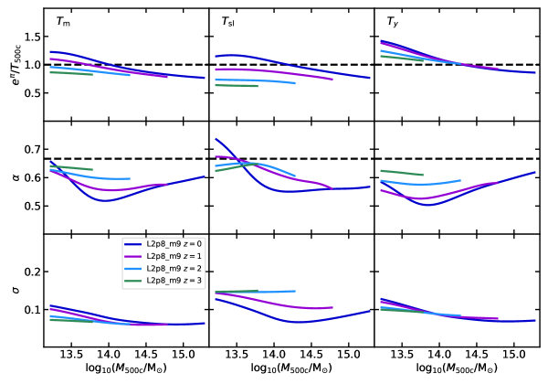
We first look at the LLR parameters for the fiducial L2p8_m9 run, shown as a function of halo mass at redshifts $z=0,1,2,3$ in Fig. 1. The temperature normalisation, $\exp(\pi)$, results are shown in the top panels. We plot this relative to $T_{\rm 500c}$ for each halo mass bin to highlight the differences between results and to remove the self-similar redshift dependence ($T\propto E(z)^{2/3}$ at fixed mass). For all 3 temperature weightings at $z=0$ (dark blue curves), we see that $T>T_{\rm 500c}$ on group scales ($M_{\rm 500c}<10^{14}\,{\rm M}_{\odot}$) but $T<T_{\rm 500c}$ for the more massive clusters. Consequently, in the middle panels we see that the local slope, $\alpha$, is smaller than the self-similar scaling (2/3) except for the spectroscopic-like temperature at the lowest masses, where this is no longer a reliable X-ray proxy. On group scales, the slope becomes flatter with increasing mass, reaches a minimum around $M_{\rm 500c}\sim 10^{14}\,{\rm M}_{\odot}$, then starts increasing again but never quite reaches the self-similar value in massive clusters (we will discuss this further, below). The scatter (bottom panels) is typically quite low ($\sigma\sim 0.05-0.1$) and is largest in the low-mass groups. This mass dependence is expected from non-gravitational processes (radiative cooling and subsequent feedback) that result in gas with higher entropy (hotter and less dense) in groups than in clusters.

Comparing the 3 temperature weightings (different columns), the SZ $y$-weighted temperature is higher in groups than the mass and spectroscopic-like values, but closest to the gravitational temperature in massive clusters. The first point means that the gas with the highest pressure in groups is hotter, as can be expected from the effects of thermal feedback, heating the densest gas and ejecting it from the halo, a process that is more effective in lower mass objects with shallower gravitational potentials. On the other hand, the spectroscopic-like temperature is most affected by cooler (but still hotter than 0.1 keV), denser gas. Such gas becomes more prevalent in more massive clusters which likely explains why the slope increases more gradually with mass on cluster scales than for the other temperature measures (e.g. see Barnes et al. 2017).

The results at higher redshift span a narrower range in mass due to the paucity of high-mass objects there. However, the 2.8 Gpc box is still sufficiently large to contain reasonable numbers ($>10$) of clusters ($M_{\rm 500c}>10^{14}\,{\rm M}_{\odot}$) at $z=2$ and high-mass groups ($10^{13.5}<M_{\rm 500c}/{\rm M}_{\odot}<10^{14}$) at $z=3$, making it useful for predicting the properties of high redshift objects in future deep cluster surveys. In all 3 temperature cases, looking at group scales, the normalisation is lower at higher redshift, i.e. the evolution is slower than self-similar, or, at fixed mass, objects at higher redshift are colder than expected from gravitational heating. The SZ temperature normalisation evolves closest to the self-similar rate (and is almost perfectly self-similar on cluster scales at $z<2$) whereas the spectroscopic-like temperature is the least self-similar. The slope moves closer to the self-similar value at higher redshift while the scatter is almost constant with redshift in the mass-weighted and $y$-weighted cases (spectroscopic-like temperatures show more scatter at higher redshift but again, these results are not reliable on group scales).

Our results are qualitatively consistent with those found by Lee et al. (2022) who analysed temperature-mass relations for the 3 weightings applied to 4 different simulation sets at $z=0-1.5$. Temperature-mass relations from FLAMINGO simulations at $z=0-2$ are also presented in Braspenning et al. (2023). There, the median mass-weighted temperature is plotted against halo mass and the results are shown to be in good agreement with X-ray observations at $z<0.6$.

3.3 Other models

Figure 2: Temperature-mass relations for runs that are calibrated to shifted observed cluster hot gas fractions (by the indicated number of $\sigma$ in the run label). Details are as in Fig. 1.

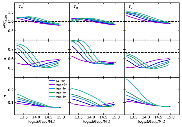
We repeated the above analysis on the full range of FLAMINGO L1 runs with hydrodynamics at $z=0$. For the runs that vary the cosmological model (including the neutrino component) we find, reassuringly, almost no change in the LLR parameters for the range of halo masses. For runs with varying resolution there are some differences at lower mass but the fiducial resolution (L1_m9) is reasonably well converged (see Appendix B). The runs with lower stellar masses (M*-1$\sigma$ and M*-1$\sigma$_fgas-4$\sigma$) produce very similar results to their L1_m9 and fgas-4$\sigma$ counterparts. This is because the hot gas dominates the baryon budget in group and cluster-sized haloes.

The most significant systematic differences in the LLR parameters are found when the hot gas fractions are varied (relative to observational uncertainties), mainly driven by the strength of AGN feedback events (more energetic events, as a result of higher heating temperature, lead to lower gas fractions). Fig. 2 shows the LLR parameters for these runs at $z=0$ with fgas-8$\sigma$ (turquoise) using the strongest feedback and fgas+2$\sigma$ (purple) the weakest. As the gas fractions are lowered (through increasing the feedback strength), the gas, unsurprisingly, becomes hotter at fixed mass, with the SZ $y$-weighted temperatures still the highest of the three.

We also see the mass scale where the slope is at a minimum increase when the gas fractions are lowered. A similar result was seen in the cosmo-OWLS simulations with varying AGN heating temperatures, studied by Le Brun et al. (2014), and is due to the effect of the AGN feedback on the entropy of the gas. At the lowest masses ($M_{\rm 500c}\sim 10^{13}\,{\rm M}_{\odot}$), the average mass-weighted temperatures are similar across the 5 gas fraction models (as can be seen from the normalisation, where the models also have $e^{\pi}>T_{\rm 500c}$, i.e. the intragroup gas is hotter than the gravitational temperature). Here, the feedback is effective at heating and ejecting gas from the halo since the AGN heating temperature, $\Delta T_{\rm AGN}\gg T_{\rm 500c}$. As halo mass increases towards cluster scales (and $T_{\rm 500c}\rightarrow\Delta T_{\rm AGN}$), the impact of the feedback on the gas temperature reduces, correspondingly leading to a decrease in the temperature ratio $e^{\pi}/T_{\rm 500c}$ and the slope, $\alpha$, also decreases. Eventually, the slope starts increasing again as the temperature becomes more and more dominated by gravitational heating at the largest masses. This transition occurs at a larger halo mass for a run with lower gas fractions due to its larger $\Delta T_{\rm AGN}$ value.

Models with lower gas fractions/stronger feedback also produce more scatter, especially in groups, and this also reaches a minimum value at a larger halo mass. The scatter is particularly large for the strongest feedback case (fgas-8$\sigma$) due to groups with very high temperatures. However, the scatter is much less model dependent for the most massive clusters where gravitational heating dominates.

Another set of runs with varying baryonic physics are those that use jet (i.e. directed kinetic) feedback rather than thermal feedback for the AGN. These models (Jet and Jet_fgas-4$\sigma$) produce qualitatively similar results to their respective thermal feedback models (L1_m9 and fgas-4$\sigma$) with the jet models producing slightly (up to around 10 per cent or so) lower temperatures and scatter on group scales. This is probably due to incomplete thermalization of feedback energy, possibly linked to the lower mass objects being less well resolved.

4 Radial Profiles and Hydrostatic Masses

Results in the previous section showed that the global SZ $y$-weighted temperatures are higher than both mass-weighted and X-ray spectroscopic-like temperatures at fixed halo mass, and vary with redshift at a rate that is closest to the self-similar expectation. These results are in agreement with previous work using smaller samples (e.g. Lee et al., 2022). We also found the temperatures to be sensitive to variations in cluster gas fractions (primarily driven by AGN feedback strength) but insensitive to variations in galaxy stellar masses and the underlying cosmological/neutrino model.

We now investigate whether the use of relativistic SZ temperatures can reduce the hydrostatic mass bias in massive clusters; for this we require the $y$-weighted radial temperature profiles. For SZ-based data where gas thermal electron pressure profiles can also be extracted (from Compton-$y$ profiles), it is appropriate to express the hydrostatic mass as a function of temperature and pressure using the following version of the hydrostatic equilibrium equation

$$M(<r)=-{k_{\rm B}\over G\mu m_{p}}\,\left[r\,T\,{{\rm d}\ln P\over{\rm d}\ln r}\right],$$ (23)

where the term in square brackets is a function of the radius $r$ and $P$ can be either the total or the electron thermal pressure since the mass depends on the relative differential ${\rm d}\ln P={\rm d}P/P$. We assume $\mu=0.59$ here, typical of observational analyses (e.g. Eckert et al., 2019). Thus, the estimated hydrostatic mass, $M_{\rm 500c,hse}$, requires both the local temperature and local pressure gradient at $R_{\rm 500c,hse}$; we will outline the procedure below and refer the reader to Braspenning et al. (2023) for a more detailed study of the ICM profiles in comparison with X-ray data. Note that we only use 3D profiles here although, in practice, the observed profiles are projected along the line-of-sight. We choose this approach as it allows us to focus on the effect of varying the temperature weighting on the hydrostatic mass estimate (and other underlying gas properties). Observational predictions will also require projection effects to be taken into account (e.g. from simulating an SZ lightcone) as well as other complications such as non-SZ sources (including the CMB) and noise. Such predictions are better focused on specific instruments (taking into account the available frequency channels, beam size etc.) and are beyond the scope of the current work. However, for now, we note that Lee et al. (2020) showed that their results for projected (cylindrical) temperature profiles produced similar differences between the different temperature weightings for the high-mass clusters relevant to this study.

For the main analysis, we use the L2p8_m9 run and only select clusters at $z=0$ with $M_{\rm 500c}>7.5\times 10^{14}\,{\rm M}_{\odot}$ (1253 objects in total; 461 clusters have $M_{\rm 500c}>10^{15}\,{\rm M}_{\odot}$). This is because the most massive clusters have the hottest gas (on average) and thus produce the largest relativistic SZ signal. Our mass limit also ensures we still have a reasonable number of objects in the smaller L1 boxes that we use for comparing results with varying models (48 clusters for L1_m9). Our choice of redshift maximises the number of high-mass systems in our box. However, in practice, observations of massive clusters are likely to be at intermediate redshift. For example, RX J1347.5-1145, as studied recently by Butler et al. (2022), is at $z=0.45$, while the CHEX-MATE Tier-2 sample (CHEX-MATE Collaboration et al., 2021) is at $0.2<z<0.6$. Therefore, we also compare our main results (hydrostatic bias parameters at $z=0$) to those at $z=0.5$; the latter sample being an order of magnitude smaller with 181 objects.

4.1 Pressure profiles

Figure 3: Top: scaled pressure profiles, plotted as $x^{3}\mathcal{P}(x)$, for the massive ($M_{\rm 500c}>7.5\times 10^{14}\,{\rm M}_{\odot}$) clusters in L2p8_m9 at $z=0$. The solid curve is the median profile while the shaded region shows the scatter (16th-84th percentiles). The dashed curve is the best-fitting generalized NFW (GNFW) model to the median profile. Bottom: results are shown relative to the best fit GNFW model.

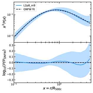
We show the (volume-weighted) thermal electron pressure profiles for the L2p8_m9 massive cluster sample in Fig. 3. The median scaled pressure profile, $\mathcal{P}=P/P_{\rm 500c}$, is plotted as a function of the dimensionless radius $x=r/R_{\rm 500c}$ (solid curve), along with the 16th to 84th percentiles (shaded region). We scale the y-axis by $x^{3}$ to highlight the relative contribution to the ICM thermal energy (or $Y$) from each radial bin as well as to highlight differences between the data and model. We do not remove any substructures when calculating the pressure profile as this would be a difficult thing to do in practice with SZ data, given the relatively low angular resolution of the observations.

The median profile is fitted with the generalized NFW (GNFW; Nagai et al. 2007b) model

$$\mathcal{P}_{\rm GNFW}(x)={P_{0}\over\left(c_{500}x\right)^{\gamma}\left[1+(c_{500}x)^{\alpha}\right]^{(\beta-\gamma)/\alpha}},$$ (24)

over the radial range $0.1<x<5$ (as shown). This range excludes the inner region so does not constrain the inner slope parameter, $\gamma$, well. Thus, following Barnes et al. (2017), we fix its value to $\gamma=0.31$ (as found by Arnaud et al. 2010) and fit the other 4 parameters $\{P_{0}=6.05\pm 0.32,c_{500}=1.77\pm 0.09,\alpha=1.48\pm 0.08,\beta=4.55\pm 0.12\}$ where the given values are for the best-fitting model (shown as the dashed curve). This produces a reasonably good fit to the median profile, in line with previous simulation studies (e.g. Nagai et al., 2007b; Kay et al., 2012; Barnes et al., 2017; Gupta et al., 2017; Planelles et al., 2017); with the largest deviations occurring beyond $R_{\rm 500c}$.

Figure 4: Scaled pressure values at 3 different radii versus halo mass. Each solid line corresponds to the median pressure while the shaded region shows the scatter (16th-84th percentiles). The median pressure of the sample is shown by the horizontal dashed line in each case. The radii were chosen to show the pressure values in the core ($x=0.1$); at intermediate radius where the scatter is minimal ($x=0.6$) and in the outskirts where the scatter is maximal ($x=3$). These results show that the scatter is not driven by an additional dependence of the pressure on cluster mass.

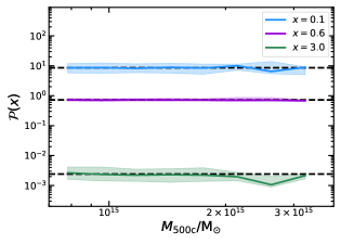
Looking at the scatter, we find it is minimal at $x\approx 0.6$ and maximal at $x\approx 3$. To check whether this scatter is due to an additional mass dependence (over and above the self-similar scaling), we show in Fig. 4 the scaled pressure values for individual clusters versus their mass at 3 different radii: $x=0.1$ (the core); $x=0.6$ (intermediate radius, minimal scatter) and $x=3$ (outskirts, maximal scatter). It is clear the scaled pressure has weak or no dependence on halo mass, with the median value close to the sample median (dashed line) in all cases except for a deviation in the most massive clusters ($M_{\rm 500c}>2\times 10^{15}\,{\rm M}_{\odot}$) at $x=0.1$ and $x=3$. The Spearman correlation coefficients are $r_{s}=(0.01,-0.007,-0.2)$ for $x=(0.1,0.6,3)$, respectively. The larger scatter at large radius is likely to be associated, at least in part, with merger shocks (see below).

Figure 5: A comparison of the median pressure profiles for clusters with $M_{\rm 500c}>7.5\times 10^{14}\,{\rm M}_{\odot}$ in the different L1 models (see text for details), relative to the L1_m9 case. The shaded region illustrates 16th-84th percentiles for L1_m9, showing that the level of cluster-to-cluster scatter is larger than the variations between models.

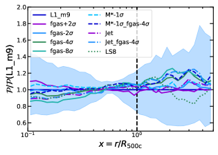
In Fig. 5, we compare the electron pressure profiles for clusters in a selection of runs with varying baryonic physics models, and the alternative LS8 cosmological model. In all cases, we see only relatively small differences ($<30$ per cent) in the pressure between models at each radius. In runs with lower hot gas fractions, driven by stronger AGN feedback, the pressure is lower in the inner region but higher in the outskirts, as may be expected from the ejection of more material to larger radii. Clusters within the LS8 run have lower pressure in the outskirts but this may be a statistical effect due to there being fewer objects above the mass limit in this run (28 clusters, compared with 48 in L1_m9).

4.2 Temperature profiles

Figure 6: Scaled temperature profiles for the massive clusters in L2p8_m9 at $z=0$, in the radial range $0.1<x<2$. The top panel shows results for the 3 different temperature weightings (mass weighted, spectroscopic-like weighted and $y$ weighted) while the bottom panel shows temperature ratios between two weightings. The solid curves are the median profiles while the shaded regions span the 16th-84th percentiles. The dashed vertical line highlights $x=1$ ($r=R_{\rm 500c}$).

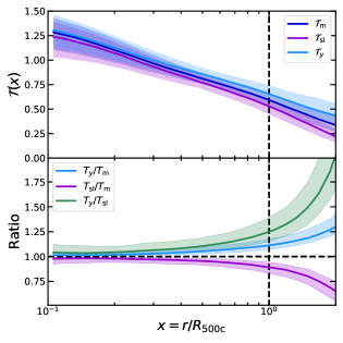
We next compare the 3D radial $y$-weighted temperature profiles to the mass-weighted and spectroscopic-like cases. Fig. 6 shows the median temperature profiles and the 16th-84th percentile regions from L2p8_m9. We restrict the radial range to $0.1<x<2$ as we are most interested in the temperatures around $x=1$ for calculating the hydrostatic masses. Furthermore, it will be much more observationally challenging to measure temperatures at $x\gg 1$ where the SZ signal is lower, the gas is cooler and the physics is more complex (e.g. the electron and ion temperatures may no longer be equal, see e.g. Fox & Loeb 1997).

In line with our $T-M$ scaling results and with previous work (Kay et al., 2008; Lee et al., 2020; Lee et al., 2022), we find that the $y$-weighted temperature, $T_{y}$, is larger than the mass-weighted temperature, $T_{\rm m}$, and the spectroscopic-like temperature, $T_{\rm sl}$, at all radii considered. Within the main cluster region these differences are relatively modest, with $T_{y}$ and $T_{\rm sl}$ being within $10-15$ per cent of $T_{\rm m}$ at $x=1$ ($r=R_{\rm 500c}$), but they increase significantly in the cluster outskirts ($1<x<2$). As can be seen in the lower panel, the $y$-weighted temperature is around twice the spectroscopic-like temperature and 25 per cent larger than the mass-weighted temperature at $x=2$. We will explore the outskirts further below, but for now, we note that the offsets around $R_{\rm 500c}$ will affect the mass estimates, given that $M\propto T$ in equation 23. Fig. 7 compares these ratios at $R_{\rm 500c}$, showing the median values and the scatter as a function of halo mass. While most of the objects are at the lower-mass end, the trend is for the highest-mass clusters to have $T_{y}/T_{\rm m}$ ratios that are around 10 per cent higher, and $T_{\rm sl}/T_{\rm m}$ ratios that are around 10 per cent lower, than the lowest-mass objects. Consequently, the median $T_{y}/T_{\rm sl}$ ratio (SZ/X-ray temperature) varies by around 20 per cent or so, over the same mass range. Spearman correlation coefficients are $r_{s}=(0.2,-0.2,0.2)$ for the $(T_{y}/T_{\rm m},T_{\rm sl}/T_{\rm m},T_{y}/T_{\rm sl})$ ratios with $M_{\rm 500c}$, respectively.

Figure 7: Ratio of temperatures measured at $R_{\rm 500c}$ versus halo mass. Solid curves show the median ratios and shaded regions the 16th-18th percentiles for each mass bin. The dashed horizontal line illustrates a ratio of unity.

Figure 8: A comparison of the median temperature profiles between different L1 models. Top: ratio of $y$-weighted temperature profiles to the fiducial (L1_m9) case. Bottom: ratio of $y$-weighted and spectroscopic-like profiles. The shaded region illustrates 16th-84th percentiles for L1_m9, showing the level of cluster-to-cluster scatter.

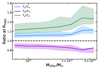
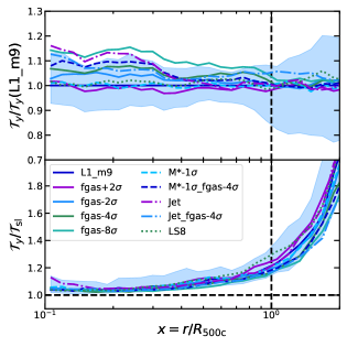
Fig. 8 shows results from comparing the temperature profiles for the different L1 models. In the top panel, we can see that relative differences in $T_{y}$ between the models and the fiducial case mainly occur within $R_{\rm 500c}$. As the hot gas fraction decreases (from increasing the thermal AGN feedback strength) the temperature within the cluster increases but the effect is mild (within 20 per cent in the extreme, fgas-8$\sigma$ case). Interestingly, the jet model, using directed kinetic AGN feedback, produces a similar increase that almost reaches 20 per cent at $0.1R_{\rm 500c}$ (see also Braspenning et al. 2023 who compared mass-weighted profiles). Beyond $R_{\rm 500c}$, $T_{y}$ is less sensitive to the feedback variations with differences less than 5 per cent. Models with varying stellar masses and cosmology/neutrinos show no discernible systematic differences in $T_{y}$ profiles (for the latter, only the LS8 case is shown here).

We also show the ratio of median $T_{y}$ and $T_{\rm sl}$ profiles for individual models in the bottom panel. These results show that the ratio is fairly insensitive to the feedback variations out to $2R_{\rm 500c}$. We can see that, in the cluster outskirts ($r>R_{\rm 500c}$) where the ratio is larger, differences between the models are smaller than the cluster-to-cluster scatter for L1_m9. This suggests the large offset between the two temperatures is a robust prediction from these simulations and so it would be interesting to test this with X-ray and (relativistic) SZ observations e.g. by stacking clusters, once it is possible to measure temperatures at these radii. However, it is not clear whether this prediction, based on simple 3D weighted temperatures, would accurately reflect the observed temperature ratio on these scales where the gas is intrinsically cooler and projection effects are likely to be significant. To test this, we would require more detailed modelling using mock observations, something that we leave to future work.

4.3 Hydrostatic masses

We now estimate individual cluster masses using equation 23. Since the individual profiles can be quite noisy (often due to substructure producing localised fluctuations), we fit model profiles to the pressure and temperature. For the pressure, we fit a 4-parameter GNFW model, fixing $\gamma=0.31$ as in Section 4.1. Here, we also restrict the radial range to $0.1<x<2$, to avoid the largest radii where deviations from a smooth profile are larger. For the temperature profile, it is common to model this using the function described in Vikhlinin et al. (2006). However, as we only need the temperature around $R_{\rm 500c}$, such a model (with up to 7 parameters) is over-complicated for our needs. Instead, we found a simpler, third-order (cubic) polynomial function to be sufficient when applied over the radial range $0.5<x<2$. These fits were made for each of the three temperature profiles ($T_{\rm m}$, $T_{\rm sl}$ and $T_{y}$).

We perform these fits for each of the 1253 clusters with $M_{\rm 500c}>7.5\times 10^{14}\,{\rm M}_{\odot}$ in L2p8_m9, using the pressure and temperature models to calculate the mass profile for $0.5<x<2$ using equation 23. From the estimated mass, we then calculate the radius at which the mean internal density, $\left<\rho\right>=500\rho_{\rm cr}$. This radius is labelled $R_{\rm 500c,hse}$ and the estimated mass $M_{\rm 500c,hse}$. The hydrostatic mass bias at $R_{\rm 500c,hse}$, $b$, is then defined through

$$1-b={M_{\rm 500c,hse}\over M_{\rm 500c}}.$$ (25)

Figure 9: Top: hydrostatic mass bias ($b$; equation 25) distributions for massive clusters in the L2p8_m9 run at $z=0$. The three histograms correspond to the different temperature profile weightings, as shown in the legend. The grey vertical line denotes $b=0$ (no bias) and the crosses illustrate the median and 16th-84th percentiles for each distribution. Bottom: as above but for the subset with the lowest pressure profile goodness-of-fit values, $\Delta(\mathcal{P})<0.02$.

Table 2: Median hydrostatic bias values and their scatter for the L2p8_m9 massive ($M_{\rm 500c}>7\times 10^{14}\,{\rm M}_{\odot}$) cluster sample and the subsample with the best GNFW pressure profile fits ($\Delta(\mathcal{P})<0.02$). Results are given for both $z=0$ (1253 clusters) and $z=0.5$ (181 clusters). Uncertainties are calculated from bootstrap re-sampling 10,000 times.

Weighting	$\left<b\right>$	$\sigma_{b}$
All clusters $z=0$:
Mass	$\phantom{-}0.091\pm 0.005$	$0.152\pm 0.006$
Spec-like	$\phantom{-}0.217\pm 0.005$	$0.151\pm 0.004$
Compton-$y$	$-0.048\pm 0.005$	$0.209\pm 0.009$
All clusters $z=0.5$:
Mass	$\phantom{-}0.107\pm 0.013$	$0.181\pm 0.014$
Spec-like	$\phantom{-}0.281\pm 0.012$	$0.139\pm 0.011$
Compton-$y$	$-0.160\pm 0.028$	$0.306\pm 0.036$
Good-fit clusters $z=0$:
Mass	$\phantom{-}0.114\pm 0.006$	$0.112\pm 0.006$
Spec-like	$\phantom{-}0.226\pm 0.007$	$0.125\pm 0.005$
Compton-$y$	$-0.009\pm 0.005$	$0.115\pm 0.005$
Good-fit clusters $z=0.5$:
Mass	$\phantom{-}0.156\pm 0.013$	$0.088\pm 0.015$
Spec-like	$\phantom{-}0.340\pm 0.022$	$0.110\pm 0.013$
Compton-$y$	$-0.036\pm 0.017$	$0.100\pm 0.018$

Figure 10: Hydrostatic mass bias, $b$, versus pressure profile goodness-of-fit statistic, $\Delta(\mathcal{P})$ (left), and halo mass, $M_{\rm 500c}$ (right), for the massive cluster sample at $z=0$. The three temperature cases are shown in different colours, with the solid lines showing the median bias and the shaded regions the 16th-84th percentiles. The green dots show results for individual clusters with $b<-0.2$ for the $y$-weighted case. The dashed vertical line is the median value of $\Delta(\mathcal{P})$ while the solid grey vertical line corresponds to $\Delta(\mathcal{P})=0.02$, the upper limit used to define the subset with good pressure profile fits.

Figure 11: Spectroscopic-like temperature (left), Compton-$y$ weighted temperature (middle) and stellar mass density (right) maps for the cluster with a large negative mass bias using $y$-weighted temperatures ($b=-2.1$). The maps show the projection of a cubic region with side length $4R_{\rm 500c}$, centred on the cluster. Pixel values are normalised to the maximum and are shown on a logarithmic scale to improve contrast. The white contours represent equal Compton-$y$ values, $\log_{10}(y/y_{\rm max})=[-2,-1.5,-1,-0.5,-0.1]$ whereas the yellow circles indicate $[1,2]R_{\rm 500c}$.

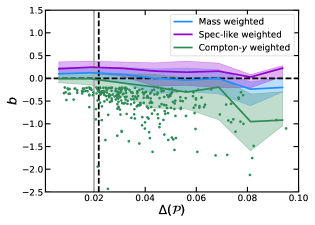
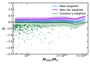
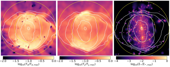
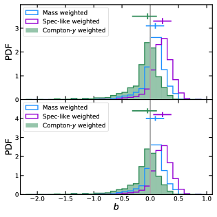
Fig. 9 (top panel) shows the distribution of $b$ values for the 3 different temperatures (the vertical grey line corresponds to $b=0$). The crosses above the histograms show the median and 16th-84th percentiles (see also Table 2). As in previous work (e.g. Biffi et al. 2016; Henson et al. 2017; Pearce et al. 2020), using the mass-weighted temperature profile results in a slightly smaller mass on average (the median bias is $\left<b\right>=0.091\pm 0.005$) but the bias more than doubles when using the spectroscopic-like temperature ($\left<b\right>=0.217\pm 0.005$) as a result of the latter being biased towards denser, cooler gas. Both distributions have similar scatter, with $\sigma_{b}\approx 0.15$ where $\sigma_{b}$ is defined to be half the difference between the 16th and 84th percentile $b$ values. On the other hand, using the $y$-weighted temperature results in a lower bias with $\left<b\right>=-0.048\pm 0.005$ but larger scatter, with $\sigma_{b}=0.21\pm 0.01$. This systematic shift in $\left<b\right>$ is expected given that $T_{y}$ is larger than the other two measures. The larger scatter is mainly due to the tail of low $b$ values (the lowest value, an extreme outlier, has $b=-2.4$). While this tail is present in all 3 distributions, it is most prominent in the $y$-weighted case, suggesting its origin must be related to the thermal pressure of the gas around $R_{\rm 500c}$.

To investigate this tail, we calculate a goodness-of-fit statistic for the GNFW fit to the pressure profile for each cluster

$$\Delta(\mathcal{P})=\sqrt{\frac{1}{N_{\rm bins}}\sum_{i=1}^{N_{\rm bins}}\left[\log_{10}\left(\mathcal{P}/\mathcal{P}_{\rm GNFW}\right)\right]^{2}},$$ (26)

where $N_{\rm bins}=26$ is the number of radial bins in the range $0.1<x<2$ used for the GNFW fit. We plot $b$ versus $\Delta(\mathcal{P})$ for the massive cluster sample in the left panel of Fig. 10. This shows that clusters with higher $\Delta(\mathcal{P})$ values (poorer pressure profile fits) tend to have larger $b$ scatter. This is particularly significant in the $T_{y}$ case where we additionally show the individual clusters with the most negative bias values ($b<-0.2$) as dots. We also note an overall trend in the median $b$ decreasing with increasing $\Delta(\mathcal{P})$; the Spearman coefficients are $r_{s}=(-0.2,-0.1,-0.3)$ when using $T_{\rm m},T_{\rm sl},T_{y}$, respectively. This confirms our expectation that the tail of negative $b$ values primarily contains objects with poor pressure profile fits.

We also show the $b$ values as a function of halo mass in the right panel of Fig. 10. There is a mild positive correlation in the $T_{\rm sl}$ case ($r_{s}=0.11$), as seen in previous work (e.g. Barnes et al., 2021), but this is considerably weaker in the other two cases ($r_{s}=0.03$ for $T_{\rm m}$ and $r_{s}=-0.03$ for $T_{y}$). The scatter shows no obvious trend with halo mass; clusters with $b<-0.2$ are found across our (limited) halo mass range but are more common at lower mass where there are more objects in total.

An example of a cluster with a poor pressure profile fit ($\Delta(\mathcal{P})\approx 0.08$) and large, negative $y$-weighted bias ($b=-2.1$) is shown in Fig. 11. Each panel shows, from left to right, $T_{\rm sl}$, $T_{y}$ and stellar mass density maps, projected down one axis of a cube, centred on the cluster, with side length $4R_{\rm 500c}$. White contours illustrate Compton-$y$ values and the yellow circles $[1,2]R_{\rm 500c}$. In this case (and typically for clusters with large $\Delta(\mathcal{P})$ values) there is clear evidence of dynamical activity: the stellar density map shows a double peak along the vertical direction, while the gas shows regions of large pressure gradients and high temperature perpendicular to this direction, associated with merger shocks. Note that these shocks occur between $1-2R_{\rm 500c}$ (between the two yellow circles) and hence affect the pressure profile fit.

Figure 12: Median pressure (top) and temperature (bottom) profiles for all massive clusters in L2p8_m9 (blue), compared to the subsamples with good (purple) and bad (green) fits to their GNFW model pressure profiles.

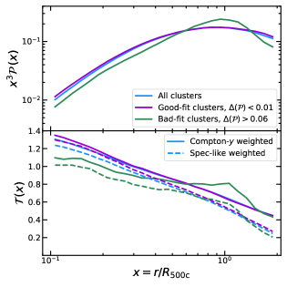
More quantitatively, we show median pressure and temperature profiles in Fig. 12 for all clusters (blue), clusters with good pressure profile fits ($\Delta(\mathcal{P})<0.01$; purple) and clusters with bad fits ($\Delta(\mathcal{P})>0.06$; green). In the bottom panel, solid curves are for the $y$-weighted temperature and dashed curves for the spectroscopic-like temperature. The median pressure profile for the bad-fitting clusters is significantly different from the other two at nearly all radii. The pressure is lower at $r<0.5R_{\rm 500c}$ and up to 30 per cent higher at $r\approx R_{\rm 500c}$. The $y$-weighted temperature profile shows similar behaviour whereas the effect on the spectroscopic-like temperature profile is smaller in the outskirts (around 10 per cent enhancement at $R_{\rm 500c}$). Consequently, it is these local increases in pressure and $y$-weighted temperature, associated with the merger shocks seen in Fig. 11, that lead to the tail of low (negative) $b$ values.

Removing clusters with the largest pressure deviations (relative to the GNFW model) would therefore be a simple, if not optimal, way to reduce the scatter in the mass bias. We demonstrate this by taking the subset of 563 clusters with $\Delta(\mathcal{P})<0.02$, close to the sample median (see Fig. 10). The resulting $b$ distributions for this subsample are shown in the lower panel in Fig. 9, with $\left<b\right>$ and $\sigma_{b}$ values listed in Table 2. As expected, removing these clusters has the largest impact on the $y$-weighted case, where the median bias reduces to $\left<b\right>=-0.009\pm 0.005$ and the scatter reduces by a factor of two, to $\sigma_{b}=0.115\pm 0.005$. For the mass-weighted case we find $\left<b\right>=0.114\pm 0.006$ and $\sigma_{b}=0.112\pm 0.006$, while for the spectroscopic-like case $\left<b\right>=0.226\pm 0.007$ and $\sigma_{b}=0.125\pm 0.005$. In these latter two cases, the median bias is slightly higher than for the full mass-limited sample while the scatter has decreased by only around 20-25 per cent.

While eliminating clusters with poor fits is an effective measure, it is not desirable for many applications where statistically-complete samples are required, most obviously when using cluster number counts to constrain cosmological parameters. Additionally, removing these objects could also introduce biases, e.g. in determining the distribution of cluster morphology or the range of thermodynamic profiles. Alternative, more optimal approaches may be possible such as measuring the profiles only along directions orthogonal to the merger axis, or using the azimuthal median profile rather than the mean. The latter, in particular, is a promising method to reduce the effect of shocks (or other discontinuities) that lead to local fluctuations and/or reduce gas clumping (e.g. Zhuravleva et al. 2013; Eckert et al. 2015; Towler et al. 2023). We leave such a study to future work as it requires a detailed analysis of the SZ maps and the deprojection of these data to infer the underlying 3D profiles.

4.4 Hydrostatic bias in different models

Figure 13: Median hydrostatic bias parameter, $\left<b\right>$ (top), and scatter, $\sigma_{b}$ (bottom), for massive ($M_{\rm 500c}>7.5\times 10^{14}\,{\rm M}_{\odot}$) clusters in various L1 runs labelled along the x-axis. The symbols represent the different temperature weightings while error bars are the 1$\sigma$ uncertainties from bootstrap re-sampling 10,000 times. Horizontal bands represent results (and uncertainties) from the main L2p8_m9 sample. The $\sigma_{b}$ bands for the mass-weighted and spectroscopic-like temperatures overlap.

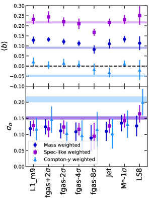
We compare the median bias, $\left<b\right>$, and scatter, $\sigma_{b}$, for various L1 runs in Fig. 13. The former values are shown in the top panel along with the corresponding result from the L2p8_m9 run as a horizontal band. For all models shown, we see the same separation in $\left<b\right>$ between the different temperature cases; using $T_{\rm sl}$ gives the largest bias and $T_{y}$ the smallest. For $T_{\rm sl}$, results for L1_m9 are similar to L2p8_m9 but the $T_{\rm m}$ and $T_{y}$ results increase with the latter now consistent with no bias. For a given temperature case, small differences are seen for the runs with varying gas fractions. As the gas fraction decreases (mainly due to stronger AGN feedback), the bias parameter goes down slightly. Runs with jet feedback, lower stellar masses or lower $S_{8}$ also produce similar bias parameters to the fiducial case.

The scatter in the bias parameter (bottom panel) is reasonably consistent between all runs and between different temperature weightings. However, the scatter for the $y$ weighted case is around a factor of two lower than for the larger L2p8_m9 box. The $b$ distribution lacks the tail to negative $b$ values seen for L2p8_m9 and also leads to a larger median value. The result cannot be explained by the larger box containing more massive objects as we saw earlier that the scatter did not vary with halo mass (Fig. 10). Instead, this suggests that the higher frequency of extreme clusters is a feature of the larger volume of the L2p8_m9 run, better able to describe the non-Gaussian statistics of massive clusters.

4.5 Hydrostatic mass bias at higher redshift

Figure 14: As in Fig. 9 but showing the $b$ distributions for massive clusters at $z=0.5$.

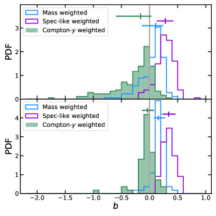
As stated above, our main results are presented at $z=0$ to maximise the sample size but many observed massive clusters will be located at intermediate redshifts (e.g. $z\sim 0.3-0.5$) as a result of the trade-off between the increase in volume and a lack of massive clusters existing at higher redshift (to illustrate this last point, we only find one cluster with $M_{\rm 500c}>10^{15}\,{\rm M}_{\odot}$ in L2p8_m9 at $z=1$). We thus restrict our redshift study to $z=0.5$ where there are 181 objects above our mass limit.

Fig. 14 shows the equivalent set of results to Fig. 9 but for $z=0.5$. We also provide median bias ($\left<b\right>$) and scatter ($\sigma_{b}$) values in Table 2. For all 3 cases, the magnitude of the median bias increases at $z=0.5$ over $z=0$. However, the changes in the $y$-weighted bias are significantly larger than for the other two cases, with the median value around three times larger and the scatter increasing by around 50 per cent. These results are not unexpected since such massive clusters (selected above a fixed mass limit) are dynamically younger at higher redshift and are thus more likely to show signs of merger activity and shocks. We find similar trends between $b$ and $M_{\rm 500c}$, and $b$ and $\Delta(\mathcal{P})$, as at $z=0$. There is only a weak trend in $b$ with mass ($r_{s}=(-0.06,0.05,-0.1)$ for the $T_{\rm m},T_{\rm sl},T_{y}$ cases, respectively) but a stronger (anti-)correlation between $b$ and $\Delta(\mathcal{P})$ ($r_{s}=(-0.4,-0.3,-0.5)$ for the same cases). Again, restricting the sample to objects with $\Delta(\mathcal{P})<0.02$ (55 clusters), the bias for the $y$-weighted case reduces significantly with the scatter being consistent with the $z=0$ value at $1\sigma$.

4.6 A closer look at the gas in cluster outskirts

Our results have shown that, in line with previous studies, the SZ $y$-weighted temperatures are higher than the X-ray spectroscopic-like temperatures, particularly in the cluster outskirts. We have also shown that this leads to a smaller median hydrostatic mass bias around $R_{\rm 500c}$ than when the spectroscopic-like temperature is used, particularly when dynamically disturbed clusters with strong localised pressure fluctuations are excluded. It is tempting to think there is a physical reason for this reduction in bias as, away from shocks, gas with the highest thermal pressure ought to be the most hydrostatic. We investigate this here by comparing radial profiles for a few other gas properties using the same weightings as we did for the temperature.

Figure 15: Top: electron density profiles ($x^{2}n_{\rm e}$) for clusters in L2p8_m9 at $z=0$ for 3 different cases: volume weighted, spectroscopic-like weighted and $y$ weighted. Bottom: ratios between profiles with different weightings.

Figure 16: Left: radial velocity profiles for the massive clusters in L2p8_m9 at $z=0$ for 3 different cases: mass weighted, spectroscopic-like weighted and $y$ weighted. Right: 3D velocity dispersion profiles for the same cases. Ratios of the profiles are shown in the lower panels (the absolute value is taken for the radial velocity case).

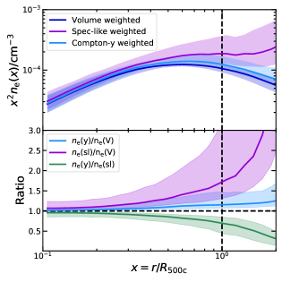
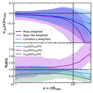
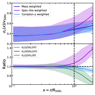
Fig. 15 shows the electron density ($x^{2}n_{\rm e}$) profiles for three different weightings. The first case is the volume-weighted electron density which has the smallest cluster-to-cluster scatter. We also show the case that uses spectroscopic-like weighting; while not an observable, it informs us of the typical electron density of gas that contributes most to $T_{\rm sl}$. At $x>0.6$, we see that $x^{2}n_{\rm e}$ is approximately constant and the ratio between this density with the volume-weighted case increases rapidly with radius. This is a result of the ICM becoming increasingly clumpy at larger radii, with the denser gas also tending to be cooler (both increasing the spectroscopic-like weight). On the other hand, the $y$-weighted profile traces the volume-weighted profile more closely, to within 25 per cent or so, out to $x=2$. Thus, the gas in the outskirts with the highest pressure (and thus the largest $y$ weighting) has lower density and higher temperature than the gas with the highest spectroscopic-like weighting. On larger scales (not shown), we find that even the $y$-weighted density becomes significantly higher than the volume-weighted case, particularly around $5R_{\rm 500c}$, where we expect the accretion shock to be located; see e.g. Aung et al. (2021).

This result suggests that the high-pressure gas, traced by the SZ effect, may be more hydrostatic in the outskirts, on average. To test this, we also consider the weighted hot gas radial velocity and 3D velocity dispersion profiles as both should be reduced for the $y$-weighted gas, relative to the other weightings. Fig. 16 confirms this, where we have scaled the velocities to the circular velocity, $v_{\rm 500c}$, of each halo at $R_{\rm 500c}$. In the left panel, the median radial velocities are always negative, as expected for infalling gas. In all cases, these values are small ($<$10 per cent of $v_{\rm 500c}$) within $R_{\rm 500c}$. At larger radii, the radial velocity magnitudes are larger but the $y$-weighted median remains within 10 per cent of $v_{\rm 500c}$ or so, at $x=2$. On the other hand, the spectroscopic-like-weighted gas has a significantly larger radial velocity magnitude, over twice that of the mass-weighted case (and around 4 times that of the $y$-weighted case) at $x=2$. Similarly, in the right panels, the 3D velocity dispersions are similar to each other within $R_{\rm 500c}$, with $\sigma_{v}$ increasing with radius, signifying an increase in non-thermal pressure. In the outskirts, the median values for the three weightings diverge, with the $y$-weighted value being the smallest and the spectroscopic-like-weighted value the largest (the former is around two thirds of the latter at $x=2$).

5 Summary and Conclusions

In this paper, we have used the large-volume FLAMINGO cosmological simulations (Schaye et al., 2023; Kugel et al., 2023) to study how using the Compton $y$-weighted temperature, an observable that can be extracted from the relativistic SZ spectral distortion in massive clusters, impacts upon measurements of the hydrostatic mass bias. We also study how this temperature compares with the mass-weighted and spectroscopic-like temperatures, the latter being a proxy for the X-ray spectroscopic temperature, both within clusters and in their outskirts. The FLAMINGO simulations have been particularly beneficial as they have allowed us to (a) select, for the first time, a large ($\sim 10^{3}$ objects) mass-complete sample of massive ($M_{\rm 500c}>7.5\times 10^{14}\,{\rm M}_{\odot}$) clusters from a single hydrodynamical simulation; and (b) study the impact of varying the cosmological and subgrid (feedback) models relative to the fiducial case that is calibrated to observations. The fiducial model has also previously been shown to produce results in good agreement with observed X-ray cluster scaling relations and radial profiles (Braspenning et al., 2023). Here, we summarise our main results:

• Compton-$y$-weighted temperatures are higher than mass-weighted and spectroscopic-like temperatures at fixed mass, in line with previous work, and evolve self-similarly with redshift out to at least $z=1$ (Fig. 1). These temperatures are higher when clusters contain lower gas fractions (mainly as a result of stronger AGN feedback). The temperature scatter at fixed mass is insensitive to these changes in high mass clusters but increases with feedback strength in groups (Fig. 2).

• Pressure profiles are generally well characterized by the GNFW model for massive clusters (Fig. 3). Cluster-to-cluster scatter is minimal at $r\approx 0.6R_{\rm 500c}$ and maximal at $r\approx 3R_{\rm 500c}$. The profiles are self-similar at these scales to good approximation (Fig. 4). Models with stronger AGN feedback have slightly lower pressure in the core and higher pressure in the outskirts, as a result of more gas being ejected (Fig. 5).

• $y$-weighted temperatures are similar to spectroscopic-like temperatures around the edge of the core ($r\approx 0.1R_{\rm 500c}$) but diverge at larger radii and are around twice as high in the outskirts ($r\approx 2R_{\rm 500c}$; Fig. 6). At $R_{\rm 500c}$, appropriate for mass estimates, $T_{y}$ is around 25 per cent higher than $T_{\rm sl}$ and increases gradually with mass (Fig. 7). We find an increase in $T_{y}/T_{\rm sl}$ with radius that is insensitive to variations in baryonic physics and cosmology (Fig. 8), making it a robust prediction that can be tested with X-ray and SZ observational data e.g. by stacking clusters to measure the signal in the outskirts.

• Hydrostatic masses with $y$-weighted temperatures are less biased, on average, than when using spectroscopic-like temperatures but have larger scatter (Fig. 9). The latter is due to clusters with large pressure and $T_{y}$ fluctuations close to $R_{\rm 500c}$ (Fig. 12) that, on inspection, are associated with merger activity (Fig. 11). Such clusters tend to have poorly fitting GNFW models (Fig. 10) and when only clusters with good fits are considered, the scatter reduces considerably. At intermediate redshift ($z=0.5$) the median bias is around three times larger as a result of massive clusters being dynamically younger (Fig. 14) but is consistent with the $z=0$ result when poorly fitted clusters are removed.

• The median bias and scatter are similar for all models run with a 1 Gpc box and varying baryonic physics and cosmology (Fig. 13) but show significant deviations from the main results that used a larger (2.8 Gpc) box. The former do not contain as many extreme, merging objects so is likely a statistical effect caused by the non-Gaussian nature of the density field in relation to rare, massive objects. It is therefore evident from this example that caution should be applied when using cosmological simulations with modest box sizes to calculate probabilities of rare events like merging massive clusters (extreme value statistics).

• Focusing on the gas in cluster outskirts ($1<r/R_{\rm 500c}<2$), Compton-$y$ (pressure) weighting yields lower electron density (Fig. 15), radial velocity and velocity dispersion (Fig. 16) than X-ray (spectroscopic-like) weighting, as well as higher temperatures. These results suggest the SZ temperature is a more sensitive tracer of gas that is smoother and more hydrostatic than the X-ray temperature, which is affected by cooler, clumpier gas.

In conclusion, our study shows that the relativistic SZ effect in clusters is an important method for independently measuring the ICM temperature. Firstly, there is the prospect of measuring cluster masses with SZ data only; our results show these masses to be unbiased if pressure fluctuations associated with mergers/shocks can be accounted for. Secondly, our work shows that comparing SZ and X-ray temperatures in cluster outskirts ought to be informative for probing the gas structure. The ability to measure the temperature of the ICM with SZ observations may also be useful as an independent calibration measure, as temperature measurements from different X-ray telescopes differ at the level of 10-20 per cent (e.g. Schellenberger et al., 2015; Wallbank et al., 2022).

Existing attempts of measuring SZ temperatures are still quite rare but future telescopes with millimetre/sub-millimetre capability are including the relativistic SZ effect in their science case, e.g. FYST/CCAT-prime (Stacey et al., 2018); AtLAST (Ramasawmy et al., 2022; Di Mascolo et al., 2024). With such instruments, it should be possible to measure relativistic temperatures at different scales in a reasonable amount of observing time (Perrott, 2023) and start to test the above predictions. On the theoretical side, we will also require more realistic, mock X-ray and SZ data from simulations to test whether our predictions hold under more realistic observational conditions.

Data Availability

The data used in the plots can be made available on reasonable request to the corresponding author. The FLAMINGO data will eventually be made publicly available when it is practically feasible to do so. In the meantime, anyone interested in using the data can contact the corresponding author.

Appendix A Higher order terms

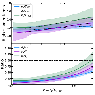
Here, we briefly look at the radial profiles of the functions used for the higher (2nd, 3rd and 4th) order terms in the Taylor expansion of the relativistic spectral distortion $f(\nu,T_{\rm e})$ about $T_{y}$ (Chluba et al., 2013). As discussed in Section 2.1, this choice of pivot temperature means that the linear term vanishes and the $k$th order terms are proportional to the following temperature moments

$$\mathcal{F}_{k}=\left<(T_{\rm e}-T_{y})^{k}\right>,$$ (27)

where $\left<\right>$ corresponds to the y-weighted average used in equation 9. For $k=2,3\,\&\,4$, we can write the respective functions as

$$\mathcal{F}_{2}\equiv\sigma_{y}^{2} = \left<T_{\rm e}\right>^{2}-T_{y}^{2}$$

$$\mathcal{F}_{3}\equiv\rho_{y}^{3} = \left<T_{\rm e}^{3}\right>+2T_{y}^{3}-3T_{y}\left<T_{\rm e}\right>^{2}$$

$$\mathcal{F}_{4}\equiv\kappa_{y}^{4} = \left<T_{\rm e}^{4}\right>-3T_{y}^{4}+6T_{y}^{2}\left<T_{\rm e}\right>^{2}-4T_{y}\left<T_{\rm e}\right>^{3},$$ (28)

where $\sigma_{y},\rho_{y},\kappa_{y}$ all have dimensions of temperature. (Note that these functions will be related to the variance, skewness and kurtosis of the temperature distribution at a given radius, respectively.) Thus, to fourth order, we have

$$\int\!\tilde{y}f(\nu,T_{\rm e}){\rm d}V\approx Y\left[f(\nu,T_{y})+\tfrac{1}{2}\partial^{2}\!f\sigma_{y}^{2}+\tfrac{1}{6}\partial^{3}\!f\rho_{y}^{3}+\tfrac{1}{24}\partial^{4}\!f\kappa_{y}^{4}\right].$$ (29)

Figure 17: Radial dependence of the higher order terms in the relativistic SZ expansion (see text for details). Top: results are scaled to $T_{\rm 500c}$ for each cluster. The dotted lines are least-squares fits to the median profiles over the radial range $0.15<r/R_{\rm 500c}<2$. Bottom: ratio of each higher order term to $T_{y}$.

Table 3: Values for the intercept, $A$, and slope, $B$, for linear least-squares fits to the variation in higher-order terms, relative to $T_{\rm 500c}$, with radius.

Term	$A$	$B$
$\sigma_{y}/T_{\rm 500c}$	$0.22$	$0.10$
$\rho_{y}/T_{\rm 500c}$	$0.26$	$0.22$
$\kappa_{y}/T_{\rm 500c}$	$0.38$	$0.25$

We evaluate the temperature moments, $\sigma_{y},\rho_{y},\kappa_{y}$, as a function of radius and show the results in Fig. 17. The top panel shows that, unlike $T_{y}$, these higher order functions increase with radius, i.e. the ($y$-weighted) temperature distribution is becoming increasingly broad and asymmetric on larger scales. Relative to $T_{y}$, these terms are small (around 10 per cent in the core, $x=0.1$) but become significant in the outskirts ($x=1-2$), as shown in the bottom panel. A similar result was found by Lee et al. (2020) for the temperature scatter, $\sigma_{y}$, using the BAHAMAS+MACSIS simulations (McCarthy et al., 2017; Barnes et al., 2017). We provide a simple linear least-squares fit to the radial profiles in the form $Y=A+B\log_{10}(r/R_{\rm 500c})$ where $Y=\{\sigma_{y},\rho_{y},\kappa_{y}\}/T_{\rm 500c}$ and the fit is performed over the radial range $0.15<r/R_{\rm 500c}<2$. Values for $A$ and $B$ are given in Table 3 with the fits shown as dotted lines in the top panel of Fig. 17.

Figure 18: Ratio of median higher order profiles in the varying L1 models to the fiducial L1_m9 case

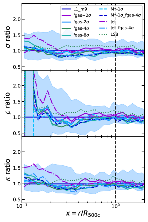
We also compare the radial profiles of the higher order terms between models in Fig. 18. As with the pressure and temperature profiles, the differences between models are typically small, although the kinetic AGN feedback Jet model produces larger temperature scatter (and higher-order effects) in the central region ($x<0.2$ or so).

Note that each higher order ($k$) term would also need to be weighted by $\partial^{k}f/k!$ when calculating the full relativistic signal at a given frequency. This can be achieved using numerical codes like szpack Chluba et al. (2012), something we will address in future work.

Appendix B Results at varying resolution

Table 4: Fiducial runs with varying box-size and resolution. Column 1 gives the run label; 2 and 3 the baryon and particle numbers respectively; 4 the comoving box-size and 5 the gas particle mass. Note that runs at varying resolution are calibrated separately to the observational data.

Label	$N_{\rm b}$	$N_{\nu}$	$L$	$m_{\rm gas}$
			(cGpc)	${\rm M}_{\odot}$
L2p8_m9	50403	28003	2.8	$1.07\times 10^{9}$
L1_m8	36003	20003	1	$1.34\times 10^{8}$
L1_m9	18003	10003	1	$1.07\times 10^{9}$
L1_m10	9003	5003	1	$8.56\times 10^{9}$

The FLAMINGO simulations include L1 runs at varying resolution; here we compare some of our key results for the runs with gas particle masses 8 times higher (L1_m10) and lower (L1_m8) than the fiducial case (L1_m9); see Table 4. Note these runs were calibrated separately (to the same observables) so their sub-grid model parameters vary (see Kugel et al. 2023 and Schaye et al. 2023 for details). As discussed in Schaye et al. (2015), this can be classed as a weak convergence study.

Figure 19: Temperature-mass relations for the L1 box with varying mass resolution (L1_m10, L1_m9, L1_m8 are low, standard, and high resolution runs, respectively). Details are as in Fig. 1.

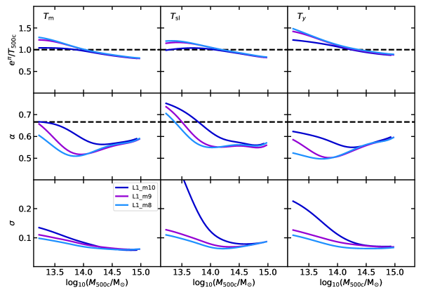
Fig. 19 shows the LLR parameters for the temperature-mass relations at $z=0$. The normalisation parameter (top panel) is converged for all 3 runs on cluster scales ($M_{\rm 500c}>10^{14}\,{\rm M}_{\odot}$), whereas on group scales, the low-resolution L1_m10 run under-predicts the temperature by up to 30 per cent or so (this is likely due to stellar feedback being switched off in this run which also predicts larger gas fractions in lower-mass groups which are below the calibration scale; see Fig. 10 in Schaye et al. 2023). The slope and scatter (middle and bottom panels) show larger differences at low mass, particularly between the the L1_m10 and L1_m9 models. Both the slope and scatter are smaller at higher resolution. The L1_m9 and L1_m8 runs show better agreement, with the minimum slope occuring around the same halo mass. All 3 runs come into good agreement at $M_{\rm 500c}>10^{14.3}\,{\rm M}_{\odot}$.

Figure 20: As in Fig. 5 but comparing the median pressure profile for each resolution level to the fiducial case.

Figure 21: As in Fig. 8 but comparing the median temperature profile for each resolution level to the fiducial case.

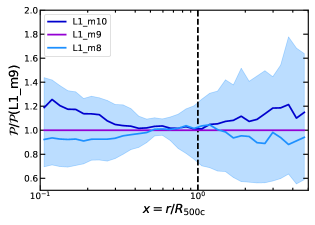
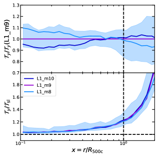
Fig. 20 compares the median pressure profiles for the massive cluster sample ($M_{\rm 500c}>7.5\times 10^{14}\,{\rm M}_{\odot}$) at the three resolution levels. As in Fig. 5, we plot the profile relative to the fiducial L1_m9 case. In general, the median profiles are very similar, with deviations only occurring in the core and far outskirts. The lower resolution L1_m10 run produces clusters with slightly higher (20 per cent) pressures in the core and far outskirts, while the higher resolution L1_m8 run only differs by up to 5 per cent or so. Importantly, for this study, the pressure profiles are well converged around $R_{\rm 500c}$, where we estimate cluster masses.

Figure 22: As in Fig. 13 but comparing the bias parameter for the runs with different resolution.

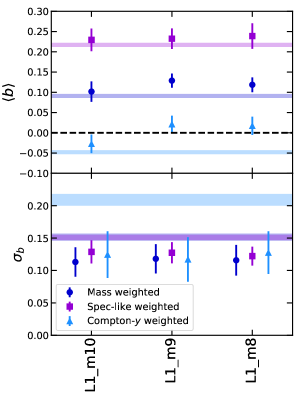
We also compare $y$-weighted temperature profiles in Fig. 21. Here, the deviations are smaller (within 10 per cent) with a higher core temperature at higher resolution. The increasing $T_{y}/T_{\rm sl}$ ratio with radius is identical in all 3 resolution cases, providing further support to the robustness of this result.

Finally, we compare median hydrostatic bias parameters, $\left<b\right>$, and scatter, $\sigma_{b}$, for the runs with varying resolution in Fig. 22. Results for all three runs are consistent with each other, with the $y$-weighted masses being unbiased, on average.

References

- Allen et al. (2004) Allen S. W., Schmidt R. W., Ebeling H., Fabian A. C., van Speybroeck L., 2004, MNRAS, 353, 457
- Allen et al. (2011) Allen S. W., Evrard A. E., Mantz A. B., 2011, ARA&A, 49, 409
- Ameglio et al. (2009) Ameglio S., Borgani S., Pierpaoli E., Dolag K., Ettori S., Morandi A., 2009, MNRAS, 394, 479
- Ansarifard et al. (2020) Ansarifard S., et al., 2020, A&A, 634, A113
- Arnaud et al. (2010) Arnaud M., Pratt G. W., Piffaretti R., Böhringer H., Croston J. H., Pointecouteau E., 2010, A&A, 517, A92
- Aslanbeigi et al. (2013) Aslanbeigi S., Lavaux G., Hajian A., Afshordi N., 2013, MNRAS, 435, 1788
- Aung et al. (2021) Aung H., Nagai D., Lau E. T., 2021, MNRAS, 508, 2071
- Barnes et al. (2017) Barnes D. J., Kay S. T., Henson M. A., McCarthy I. G., Schaye J., Jenkins A., 2017, MNRAS, 465, 213
- Barnes et al. (2021) Barnes D. J., Vogelsberger M., Pearce F. A., Pop A.-R., Kannan R., Cao K., Kay S. T., Hernquist L., 2021, MNRAS, 506, 2533
- Biffi et al. (2016) Biffi V., et al., 2016, ApJ, 827, 112
- Birkinshaw (1999) Birkinshaw M., 1999, Phys. Rep., 310, 97
- Bleem et al. (2015) Bleem L. E., et al., 2015, ApJS, 216, 27
- Booth & Schaye (2009) Booth C. M., Schaye J., 2009, MNRAS, 398, 53
- Borrow et al. (2022) Borrow J., Schaller M., Bower R. G., Schaye J., 2022, MNRAS, 511, 2367
- Bourdin et al. (2017) Bourdin H., Mazzotta P., Kozmanyan A., Jones C., Vikhlinin A., 2017, ApJ, 843, 72
- Braspenning et al. (2023) Braspenning J., et al., 2023, arXiv e-prints, p. arXiv:2312.08277
- Briel et al. (1992) Briel U. G., Henry J. P., Boehringer H., 1992, A&A, 259, L31
- Butler et al. (2022) Butler V. L., et al., 2022, ApJ, 932, 55
- CHEX-MATE Collaboration et al. (2021) CHEX-MATE Collaboration et al., 2021, A&A, 650, A104
- Chaikin et al. (2022) Chaikin E., Schaye J., Schaller M., Bahé Y. M., Nobels F. S. J., Ploeckinger S., 2022, MNRAS, 514, 249
- Challinor & Lasenby (1998) Challinor A., Lasenby A., 1998, ApJ, 499, 1
- Chiu et al. (2023) Chiu I. N., Klein M., Mohr J., Bocquet S., 2023, MNRAS, 522, 1601
- Chluba et al. (2012) Chluba J., Nagai D., Sazonov S., Nelson K., 2012, MNRAS, 426, 510
- Chluba et al. (2013) Chluba J., Switzer E., Nelson K., Nagai D., 2013, MNRAS, 430, 3054
- Di Mascolo et al. (2024) Di Mascolo L., et al., 2024, arXiv e-prints, p. arXiv:2403.00909
- Diaferio & Geller (1997) Diaferio A., Geller M. J., 1997, ApJ, 481, 633
- Durret et al. (1994) Durret F., Gerbal D., Lachieze-Rey M., Lima-Neto G., Sadat R., 1994, A&A, 287, 733
- Eckert et al. (2015) Eckert D., Roncarelli M., Ettori S., Molendi S., Vazza F., Gastaldello F., Rossetti M., 2015, MNRAS, 447, 2198
- Eckert et al. (2019) Eckert D., et al., 2019, A&A, 621, A40
- Elahi et al. (2019) Elahi P. J., Cañas R., Poulton R. J. J., Tobar R. J., Willis J. S., Lagos C. d. P., Power C., Robotham A. S. G., 2019, Publ. Astron. Soc. Australia, 36, e021
- Elbers et al. (2021) Elbers W., Frenk C. S., Jenkins A., Li B., Pascoli S., 2021, MNRAS, 507, 2614
- Elbers et al. (2022) Elbers W., Frenk C. S., Jenkins A., Li B., Pascoli S., 2022, MNRAS, 516, 3821
- Evrard et al. (1996) Evrard A. E., Metzler C. A., Navarro J. F., 1996, ApJ, 469, 494
- Farahi et al. (2018) Farahi A., Evrard A. E., McCarthy I., Barnes D. J., Kay S. T., 2018, MNRAS, 478, 2618
- Ferland et al. (2017) Ferland G. J., et al., 2017, Rev. Mex. Astron. Astrofis., 53, 385
- Fox & Loeb (1997) Fox D. C., Loeb A., 1997, ApJ, 491, 459
- Gardini et al. (2004) Gardini A., Rasia E., Mazzotta P., Tormen G., De Grandi S., Moscardini L., 2004, MNRAS, 351, 505
- Gull & Northover (1976) Gull S. F., Northover K. J. E., 1976, Nature, 263, 572
- Gupta et al. (2017) Gupta N., Saro A., Mohr J. J., Dolag K., Liu J., 2017, MNRAS, 469, 3069
- Hahn et al. (2021) Hahn O., Rampf C., Uhlemann C., 2021, MNRAS, 503, 426
- Hansen (2004) Hansen S. H., 2004, MNRAS, 351, L5
- Henson et al. (2017) Henson M. A., Barnes D. J., Kay S. T., McCarthy I. G., Schaye J., 2017, MNRAS, 465, 3361
- Hilton et al. (2021) Hilton M., et al., 2021, ApJS, 253, 3
- Huško et al. (2022) Huško F., Lacey C. G., Schaye J., Schaller M., Nobels F. S. J., 2022, MNRAS, 516, 3750
- Itoh et al. (1998) Itoh N., Kohyama Y., Nozawa S., 1998, ApJ, 502, 7
- Jenkins (2013) Jenkins A., 2013, MNRAS, 434, 2094
- Kay et al. (2004) Kay S. T., Thomas P. A., Jenkins A., Pearce F. R., 2004, MNRAS, 355, 1091
- Kay et al. (2008) Kay S. T., Powell L. C., Liddle A. R., Thomas P. A., 2008, MNRAS, 386, 2110
- Kay et al. (2012) Kay S. T., Peel M. W., Short C. J., Thomas P. A., Young O. E., Battye R. A., Liddle A. R., Pearce F. R., 2012, MNRAS, 422, 1999
- Kennicutt (1998) Kennicutt Robert C. J., 1998, ApJ, 498, 541
- Kravtsov & Borgani (2012) Kravtsov A. V., Borgani S., 2012, ARA&A, 50, 353
- Kugel et al. (2023) Kugel R., et al., 2023, MNRAS, 526, 6103
- Lau et al. (2009) Lau E. T., Kravtsov A. V., Nagai D., 2009, ApJ, 705, 1129
- Le Brun et al. (2014) Le Brun A. M. C., McCarthy I. G., Schaye J., Ponman T. J., 2014, MNRAS, 441, 1270
- Lee et al. (2020) Lee E., Chluba J., Kay S. T., Barnes D. J., 2020, MNRAS, 493, 3274
- Lee et al. (2022) Lee E., et al., 2022, MNRAS, 517, 5303
- Mamon et al. (2013) Mamon G. A., Biviano A., Boué G., 2013, MNRAS, 429, 3079
- Mantz et al. (2014) Mantz A. B., Allen S. W., Morris R. G., Rapetti D. A., Applegate D. E., Kelly P. L., von der Linden A., Schmidt R. W., 2014, MNRAS, 440, 2077
- Markevitch et al. (1998) Markevitch M., Forman W. R., Sarazin C. L., Vikhlinin A., 1998, ApJ, 503, 77
- Mazzotta et al. (2004) Mazzotta P., Rasia E., Moscardini L., Tormen G., 2004, MNRAS, 354, 10
- McCarthy et al. (2017) McCarthy I. G., Schaye J., Bird S., Le Brun A. M. C., 2017, MNRAS, 465, 2936
- Melin & Pratt (2023) Melin J. B., Pratt G. W., 2023, arXiv e-prints, p. arXiv:2304.09041
- Mroczkowski et al. (2019) Mroczkowski T., et al., 2019, Space Sci. Rev., 215, 17
- Nagai et al. (2007a) Nagai D., Vikhlinin A., Kravtsov A. V., 2007a, ApJ, 655, 98
- Nagai et al. (2007b) Nagai D., Kravtsov A. V., Vikhlinin A., 2007b, ApJ, 668, 1
- Oppizzi et al. (2023) Oppizzi F., et al., 2023, A&A, 672, A156
- Pacaud et al. (2018) Pacaud F., et al., 2018, A&A, 620, A10
- Pariiskii (1972) Pariiskii Y. N., 1972, Azh, 49, 1322
- Pearce et al. (2020) Pearce F. A., Kay S. T., Barnes D. J., Bower R. G., Schaller M., 2020, MNRAS, 491, 1622
- Perrott (2023) Perrott Y., 2023, arXiv e-prints, p. arXiv:2310.07126
- Perrott et al. (2019) Perrott Y. C., Javid K., Carvalho P., Elwood P. J., Hobson M. P., Lasenby A. N., Olamaie M., Saunders R. D. E., 2019, MNRAS, 486, 2116
- Piffaretti & Valdarnini (2008) Piffaretti R., Valdarnini R., 2008, A&A, 491, 71
- Planck Collaboration et al. (2013) Planck Collaboration et al., 2013, A&A, 550, A131
- Planck Collaboration et al. (2016a) Planck Collaboration et al., 2016a, A&A, 594, A24
- Planck Collaboration et al. (2016b) Planck Collaboration et al., 2016b, A&A, 594, A27
- Planelles et al. (2017) Planelles S., et al., 2017, MNRAS, 467, 3827
- Ploeckinger & Schaye (2020) Ploeckinger S., Schaye J., 2020, MNRAS, 497, 4857
- Pointecouteau et al. (1998) Pointecouteau E., Giard M., Barret D., 1998, A&A, 336, 44
- Pointecouteau et al. (2005) Pointecouteau E., Arnaud M., Pratt G. W., 2005, A&A, 435, 1
- Pointecouteau et al. (2021) Pointecouteau E., et al., 2021, A&A, 651, A73
- Pratt et al. (2021) Pratt C. T., Qu Z., Bregman J. N., 2021, ApJ, 920, 104
- Ramasawmy et al. (2022) Ramasawmy J., et al., 2022, in Zmuidzinas J., Gao J.-R., eds, Society of Photo-Optical Instrumentation Engineers (SPIE) Conference Series Vol. 12190, Millimeter, Submillimeter, and Far-Infrared Detectors and Instrumentation for Astronomy XI. p. 1219007 (arXiv:2207.03914), doi:10.1117/12.2627505
- Rasia et al. (2004) Rasia E., Tormen G., Moscardini L., 2004, MNRAS, 351, 237
- Rasia et al. (2006) Rasia E., et al., 2006, MNRAS, 369, 2013
- Remazeilles et al. (2019) Remazeilles M., Bolliet B., Rotti A., Chluba J., 2019, MNRAS, 483, 3459
- Rephaeli (1995) Rephaeli Y., 1995, ARA&A, 33, 541
- Roncarelli et al. (2013) Roncarelli M., Ettori S., Borgani S., Dolag K., Fabjan D., Moscardini L., 2013, MNRAS, 432, 3030
- Rotti et al. (2021) Rotti A., Bolliet B., Chluba J., Remazeilles M., 2021, MNRAS, 503, 5310
- Ruppin et al. (2018) Ruppin F., et al., 2018, A&A, 615, A112
- Sayers et al. (2013) Sayers J., et al., 2013, ApJ, 768, 177
- Sazonov & Sunyaev (1998) Sazonov S. Y., Sunyaev R. A., 1998, ApJ, 508, 1
- Schaller et al. (2023) Schaller M., et al., 2023, arXiv e-prints, p. arXiv:2305.13380
- Schaye & Dalla Vecchia (2008) Schaye J., Dalla Vecchia C., 2008, MNRAS, 383, 1210
- Schaye et al. (2015) Schaye J., et al., 2015, MNRAS, 446, 521
- Schaye et al. (2023) Schaye J., et al., 2023, MNRAS, 526, 4978
- Schellenberger et al. (2015) Schellenberger G., Reiprich T. H., Lovisari L., Nevalainen J., David L., 2015, A&A, 575, A30
- Stacey et al. (2018) Stacey G. J., et al., 2018, in Marshall H. K., Spyromilio J., eds, Society of Photo-Optical Instrumentation Engineers (SPIE) Conference Series Vol. 10700, Ground-based and Airborne Telescopes VII. p. 107001M (arXiv:1807.04354), doi:10.1117/12.2314031
- Sunyaev & Zeldovich (1972) Sunyaev R. A., Zeldovich Y. B., 1972, Comments on Astrophysics and Space Physics, 4, 173
- Tchernin et al. (2016) Tchernin C., et al., 2016, A&A, 595, A42
- Towler et al. (2023) Towler I., Kay S. T., Altamura E., 2023, MNRAS, 520, 5845
- Umetsu (2020) Umetsu K., 2020, A&ARv, 28, 7
- Vikhlinin et al. (2005) Vikhlinin A., Markevitch M., Murray S. S., Jones C., Forman W., Van Speybroeck L., 2005, ApJ, 628, 655
- Vikhlinin et al. (2006) Vikhlinin A., Kravtsov A., Forman W., Jones C., Markevitch M., Murray S. S., Van Speybroeck L., 2006, ApJ, 640, 691
- Vikhlinin et al. (2009) Vikhlinin A., et al., 2009, ApJ, 692, 1060
- Voit (2005) Voit G. M., 2005, Reviews of Modern Physics, 77, 207
- Wallbank et al. (2022) Wallbank A. N., Maughan B. J., Gastaldello F., Potter C., Wik D. R., 2022, MNRAS, 517, 5594
- White et al. (1993) White S. D. M., Navarro J. F., Evrard A. E., Frenk C. S., 1993, Nature, 366, 429
- Wiersma et al. (2009) Wiersma R. P. C., Schaye J., Theuns T., Dalla Vecchia C., Tornatore L., 2009, MNRAS, 399, 574
- Zhuravleva et al. (2013) Zhuravleva I., Churazov E., Kravtsov A., Lau E. T., Nagai D., Sunyaev R., 2013, MNRAS, 428, 3274
- Zwicky (1933) Zwicky F., 1933, Helvetica Physica Acta, 6, 110