First combined tuning on transverse kinematic imbalance data with and without pion production constraints

Abstract

We present the first global tuning, using genie, of four transverse kinematic imbalance measurements of neutrino-hydrocarbon scattering, both with and without pion final states, from the T2K and MINERvA experiments. As a proof of concept, we have simultaneously tuned the initial state and final-state interaction models (SF-LFG and hA, respectively), producing a new effective theory that more accurately describes the data.

I Introduction

Neutrinos play a central role in advancing our understanding of physics and addressing fundamental inquiries in contemporary science. The Hyper-Kamiokande experiment [1] aims to conduct precise measurements of charge parity violation within the neutrino sector, a phenomenon believed to be closely linked to the observed matter-antimatter asymmetry in the universe. Similarly, the Deep Underground Neutrino Experiment (DUNE) [2, 3, 4, 5] promises to elucidate the neutrino mass ordering. Owing to their substantial scale, these forthcoming experiments are ideally suited for exploring novel physics phenomena, such as neutrino-less double beta decay. Whether seeking to ascertain Standard Model parameters or probing for exotic phenomena, significant enhancements in both theoretical frameworks and computational simulations of neutrino-nucleus interactions are imperative. As neutrinos interact with nucleons inside the nucleus, the interaction is subject to nuclear effects, namely the nucleon initial state and final-state interactions (FSIs). These effects are not fully understood yet and can alter the final event topology by emission or absorption of pions. Notably, the neutrino flux at DUNE yields a comparable proportion of events with and without pions in the final state, highlighting the pressing need for a generator capable of accurately describing both event topologies.

The large data samples and superb imaging capabilities of modern neutrino experiments offer us a detailed new look at neutrino interaction physics. Recently, the GENIE [6] Collaboration has made substantial progress towards a global tuning using neutrino, charged lepton and hadron scattering data, in an attempt to integrate new experimental constraints with state-of-the-art theories and construct robust and comprehensive simulations of neutrino interactions with matter. Cross-experiment and cross-topology analyses are challenging tasks as each measurement features its unique selection criteria and various other aspects, such as the neutrino flux. GENIE has built an advanced tuning framework that enables the validation and tuning of comprehensive interaction models using an extensive curated database of measurements of neutrino, charged lepton and hadron scattering off nucleus and nuclei. So far, the non-resonant backgrounds [7], hadronization [8] and the quasielastic (QE) and 2-particle-2-hole (2p2h) components [9] of the neutrino-nucleus interaction have been tuned with $\nu_{\mu}$ and $\bar{\nu}_{\mu}$ charged-current (CC) pionless (0$\pi$) data from MiniBooNE, T2K and MINERvA. A partial tune was performed for each experiment, highlighting the neutrino energy dependence on the QE and 2p2h tuned cross sections. Even though post-tune predictions enhanced the data description for each experiment, the added degrees of freedom were not sufficient to fully describe all CC0$\pi$ data and exhibited tensions with some proton observables [9]. More exclusive measurements result in additional model constraints. In addition, observables that are sensitive to targeted aspects of the complex dynamics of neutrino interactions are invaluable for model tuning. The transverse kinematic imbalance (TKI) [10, 11], a final-state correlation between the CC lepton and the handronic system, is a good example since it is sensitive to the initial-state nuclear environment and hadronic FSI. Our next step is to incorporate TKI data from experiments where various exclusive topologies at different energies are considered. This marks the first combined tuning on TKI data with and without pions in the final states and serves as the starting point of a more comprehensive tuning effort in the energy region most relevant for future accelerator-based neutrino experiments.

This paper is structured as follows: In Sec. II, we review the TKI measurements and genie models. In Sec. III, we detail the tuning considerations and procedures. Results are summarized in Sec. IV, highlighting how the data-MC discrepancy in the MINERvA-$\pi^{0}$ TKI measurement [12] is resolved while maintaining good data-MC agreement elsewhere. We conclude in Sec. V.

II TKI measurements and genie models

TKI is a methodology focused on the conservation of momentum in neutrino interactions. In essence, it involves examining the imbalance between the observed transverse momentum of the final-state particles and the expected transverse momentum from neutrino interactions with free nucleons [10, 11]. This “kinematic mismatch,” together with its longitudinal and three-dimensional variations [13, 14], and the resulting asymmetry [15], has been a crucial set of observables, establishing a pathway to extract valuable information about the participating particles and the underlying nuclear processes. Recent experimental results from neutrino experiments such as T2K [16, 17], MINERvA [18, 19, 12], and MicroBooNE [20, 21, 22, 23, 24], as well as electron scattering experiments such as CLAS [25], highlight the efficacy of TKI.

In neutrino scattering off a free nucleon, the sum of the transverse components of the final products is expected to be zero, visualized through a back-to-back configuration between the final-state lepton and hadronic system in the plane transverse to the neutrino direction. Hence, in a neutrino interaction with a nucleus, the transverse momentum imbalance, $\delta p_{\textrm{T}}$ [11], results from intranuclear dynamics, including Fermi motion and FSIs. The deviation from being back-to-back is quantified by the coplanarity angle $\delta\phi_{\textrm{T}}$, and the transverse boosting angle, $\delta\alpha_{\textrm{T}}$ [11], indicates the direction of $\delta p_{\textrm{T}}$ within the transverse plane. Furthermore, analyzing the energy and longitudinal momentum budget [13, 14] enables the conversion of $\delta p_{\textrm{T}}$ to the emulated nucleon momentum, $p_{\textrm{N}}$, providing insight into the Fermi motion; this conversion amounts to a correction on the order of $\mathcal{O}(20\%)$ [26]. In the absence of FSIs, $\delta\alpha_{\textrm{T}}$ remains uniform (except for second-order effects, such as variations in the center-of-mass energy), given the isotropic nature of the initial nucleon motion. However, as the final products propagate through the nuclear medium, they experience FSIs, thereby disturbing the isotropy and the Fermi motion peak of the $\delta\alpha_{\textrm{T}}$ and $p_{\textrm{N}}$ ($\delta p_{\textrm{T}}$) distributions, respectively. Hence, $\delta p_{\textrm{T}}$ and $p_{\textrm{N}}$ elucidate the Fermi motion details, while $\delta\alpha_{\textrm{T}}$ characterizes the FSI strength—crucial for elucidating medium effects in neutrino interactions. Moreover, a notable advantage of these observables is their minimal dependence on neutrino energy [11]. The double TKI variable, $\delta p_{\textrm{TT}}$ [10], is the projection of $\delta\vec{p}_{\textrm{T}}$ along the axis perpendicular to the lepton scattering plane (hence “double”). In addition to its use for extracting neutrino-hydrogen interactions [10, 27], it has also been applied to study nuclear effects in neutrino pion productions [12, 17]. Its equivalent in pionless production, $\delta p_{\textrm{Tx}}$, has been proposed and studied together with its orthogonal companion, $\delta p_{\textrm{Ty}}$, in MINERvA [19].

This work surveyed four TKI data sets: T2K $0\pi$ [16], T2K $\pi^{+}$ [17], MINERvA $0\pi$ [18, 19], and MINERvA $\pi^{0}$ [12] measurements. All four measurements require the presence of one CC muon and at least one proton in the final state. While the T2K-$\pi^{+}$ measurement requires exactly one $\pi^{+}$, and MINERvA-$\pi^{0}$ requires at least one $\pi^{0}$, the other two datasets require the absence of any pions. The definitions of the phase spaces for these signals are shown in Table 1.

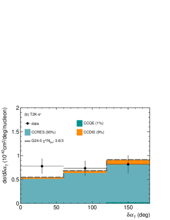
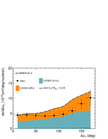
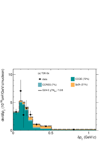
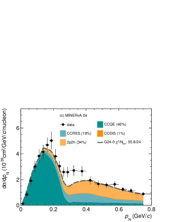
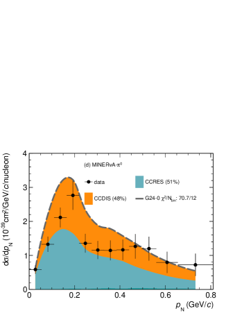
Figure 1: $\delta\alpha_{\textrm{T}}$ measurements decomposed in interaction types, compared to the nominal tune, G24-0.

Figure 2: Similar to Fig. 2 but for the $p_{\textrm{N}}$ ($\delta p_{\textrm{T}}$ for T2K-$0\pi$) measurements.

Variables	Cut Values ($p$ in $\textrm{GeV}/c$)
T2K-$0\pi$ [16]
$\vec{p}_{\mu}$ cut	$0.25<p_{\mu}$, $\cos\theta_{\mu}>-0.6$
$\vec{p}_{\textrm{p}}$ cut	$0.45<p_{\text{p}}<1.0$ , $\cos\theta_{\text{p}}>0.4$
T2K-$\pi^{+}$ [17]
$\vec{p}_{\mu}$ cut	$0.25<p_{\mu}<7$ , $\theta_{\mu}<70^{\circ}$
$\vec{p}_{\textrm{p}}$ cut	$0.45<p_{\text{p}}<1.2$ , $\theta_{\text{p}}<70^{\circ}$
$\vec{p}_{\pi}$ cut	$0.15<p_{\pi}<1.2$, $\theta_{\pi}<70^{\circ}$
MINERvA-$0\pi$ [18, 19]
$\vec{p}_{\mu}$ cut	$1.5<p_{\mu}<10$ , $\theta_{\mu}<20^{\circ}$
$\vec{p}_{\textrm{p}}$ cut	$0.45<p_{\text{p}}<1.2$ , $\theta_{\text{p}}<70^{\circ}$
MINERvA-$\pi^{0}$ [12]
$\vec{p}_{\mu}$ cut	$1.5<p_{\mu}<20$ , $\theta_{\mu}<25^{\circ}$
$\vec{p}_{\textrm{p}}$ cut	$0.45<p_{\text{p}}$

Table 1: Phase space cuts for the signals of the TKI measurements.

Given the significant physics potential of TKI measurements, a wealth of literature has emerged on the combined analysis of T2K and MINERvA CC0$\pi$ TKI data [28, 29, 30, 31, 32, 9, 33, 34]. However, model studies incorporating pion production TKI data have been notably absent. Comparing the genie predictions by G24_20i_00_000 (G24-0)—the tune from Refs. [7, 8]—shows that the model fails to accurately describe the MINERvA $\pi^{0}$ [12] TKI measurement (Figs. 2 and 2).

The genie models and tunes are detailed in the Comprehensive Model Configurations. Both the aforementioned G24-0 and the widely-used G18_10a_02_11b tunes derive from the same tuning process [7, 8], yet G24-0 distinguishes itself by three aspects: 1) incorporating a new initial state, the correlated and spectral-function-like local Fermi gas (SF-LFG) [35, 36, 37]; 2) using $z$-expansion axial-vector form factor [38] rather than the dipole form factor of the Valencia model in QE processes [39] and 3) replacing the Valencia model [40] in 2p2h processes with the SuSAv2 Model [41]. The other model components are given in Table  2. Given its simplicity and interpretability, the INTRANUKE hA FSI model (hA for short) emerges as a strong candidate for an effective model. Since the TKI measurements are sensitive to the initial state and FSI, this work investigates a partial tune of these two processes based on G24-0, in an effort to derive an effective model describing neutrino-nuclear pion production, while maintaining the efficacy with the pionless production.

Simulation domain	Model
Nuclear State	SF-LFG [35, 36, 37]
QE	Valencia [39]
2p2h	SuSAv2 [41]
QE $\Delta S=1$	Pais [42]
QE $\Delta C=1$	Kovalenko [43]
Resonance (RES)	Berger-Sehgal [44]
Shallow/Deep inelastic scattering (SIS/DIS)	Bodek-Yang [45]
DIS $\Delta C=1$	Aivazis-Tung-Olness [46]
Coherent $\pi$ production	Berger-Sehgal [47]
Hadronization	AGKY [48]
FSI	INTRANUKE hA [49]

Table 2: Model components of the nominal G24-0 tune. Processes with non-trivial $\Delta S$ and $\Delta C$ are those with strangeness and charm production, respectively.

III Tuning Initial-State and FSI models on TKI Data

This study adopts the tuning procedure outlined in Ref. [9], utilizing $N_{\textrm{par}}$ input model parameters. The objective is to identify the extremal point—that is, the optimal set of parameter values—within the parameter space that minimizes the $\chi^{2}$ between model predictions and data. Given the high dimensionality of the parameter space, conducting a brute-force, point-by-point scan on a grid is infeasible. Therefore, a sufficient number of points is randomly sampled. Each point is used to run a full simulation. The simulation output for each data observable bin is then parameterized by Professor [50] with a polynomial of the model parameters of a chosen order, $N_{\textrm{ord}}$. The minimal number of parameter sets ($N_{\textrm{s}}$) required for tuning $N_{\textrm{par}}$ parameters with an order $N_{\textrm{ord}}$ polynomial is determined by the combination formula,

$$N_{\textrm{s}}=\binom{N_{\textrm{par}}+N_{\textrm{ord}}}{N_{\textrm{ord}}}.$$ (1)

Given that $N_{\textrm{s}}$ increases factorially, caution is essential when augmenting the number of parameters or the polynomial degree. Given that our tuning incorporates all $2$ SF-LFG and $12$ hA parameters parameters (see Sec. III.2), a degree-$4$ parameterization necessitates over 6,000 generations. Hence, only up to order $4$ polynomials are explored, and it has shown to reproduce the MC predictions well as shown in Fig. 3.

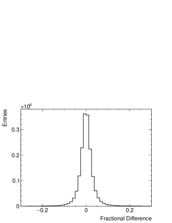
Figure 3: Fractional difference for the bin-by-bin cross sections between MC truth and the parameterized approximation with order-4 polynomials, both in the Norm-Shape (NS) [51, 52] space with AllPar. See later text for the definition of AllPar. The residual has a mean of $0.003$ and a standard deviation of $0.016$.

Furthermore, to circumvent Peelle’s Pertinent Puzzle [53], the Norm-Shape (NS) transformation prescription [51, 52] is applied. The extremal point is then found from a minimization of $\chi^{2}$ between this NS-transformed polynomial approximation and NS-transformed data. In the minimization, priors, usually based on systematic uncertainty, can be imposed on each parameter to penalize it from getting too far from its default value. The following subsections elaborate on the specific choice of measurement observables and model parameters in this work.

III.1 Data Observables

The observables for the reported differential cross sections across the four TKI measurements—T2K-$0\pi$, T2K-$\pi^{+}$, MINERvA-$0\pi$, and MINERvA-$\pi^{0}$—are detailed in Table 3. To identify the most sensitive variables, various combinations were evaluated for tuning purposes. A total of 26 combinations were assessed, with the superset comprising $\delta\alpha_{\textrm{T}}$, $\delta p_{\textrm{T}}$, $\delta\phi_{\textrm{T}}$, $p_{\textrm{N}}$, and $\delta p_{\textrm{TT}}$ (see Table 6 in Appendix .1 for all combinations). Each combination was evaluated such that non-selected variables—including proton momentum and angle ($p_{\text{p}}$ and $\theta_{\text{p}}$) [18], as well as $\delta p_{\textrm{Tx}}$ and $\delta p_{\textrm{Ty}}$ [19] in MINERvA-$0\pi$—were used solely for validation; the model is expected to accurately predict these variables post-tuning. When constructing the combinations, it was observed that $\delta\phi_{\textrm{T}}$ is strongly dependent on neutrino beam energy [11], which suppresses its sensitivity to nuclear effects. Additionally, correlations exist between various observables, notably between $\delta p_{\textrm{T}}$ and $p_{\textrm{N}}$. Therefore, determining the optimal combination is not straightforward; this study employs a criterion based on the $\chi^{2}$ with the complete (tuned plus validation) observable set (Fig. 4).

Observables	No. of bins	Combi- Superset	Combi- Best- AllPar	Combi- Best- RedPar
T2K-$0\pi$
$\delta\alpha_{\textrm{T}}$	$8$	$\checkmark$		$\checkmark$
$\delta p_{\textrm{T}}$	$8$	$\checkmark$	$\checkmark$	$\checkmark$
$\delta\phi_{\textrm{T}}$	$8$	$\checkmark$
T2K-$\pi^{+}$
$\delta\alpha_{\textrm{T}}$	$3$	$\checkmark$		$\checkmark$
$p_{\textrm{N}}$	$4$	$\checkmark$	$\checkmark$	$\checkmark$
$\delta p_{\textrm{TT}}$	$5$	$\checkmark$		$\checkmark$
MINERvA-$0\pi$
$\delta\alpha_{\textrm{T}}$	$12$	$\checkmark$		$\checkmark$
$p_{\textrm{N}}$	$24$	$\checkmark$	$\checkmark$	$\checkmark$
$\delta p_{\textrm{T}}$	$24$	$\checkmark$	$\checkmark$
$\delta\phi_{\textrm{T}}$	$23$	$\checkmark$
$p_{\textrm{p}}$	$25$
$\theta_{\textrm{p}}$	$26$
$\delta p_{\textrm{Tx}}$	$32$
$\delta p_{\textrm{Ty}}$	$33$
MINERvA-$\pi^{0}$
$\delta\alpha_{\textrm{T}}$	$9$	$\checkmark$		$\checkmark$
$p_{\textrm{N}}$	$12$	$\checkmark$	$\checkmark$	$\checkmark$
$\delta p_{\textrm{TT}}$	$13$	$\checkmark$		$\checkmark$

Table 3: Observables of the TKI measurements and their binning. Those with “$\checkmark$”’s are used for tuning, while those without are for the respective validation. See later text for the definitions of Combi-Best-RedPar and Combi-Best-AllPar.

Figure 4: Change of $\chi^{2}$ calculated for the full (i.e., tuned plus validation) observable set as a function of the tuned combination (cf. Table 6 in Appendix .1). The two model parameter sets (AllPar and RedPar, see later text for definitions) are compared and it can be seen that the respective minima happen at Combi-15 and 26.

III.2 Model Parameters

As outlined in Sec. II, we focus exclusively on the currently tunable parameters within the SF-LFG and hA models. Therefore, $14$ parameters (collectively referred to as the AllPar set) are utilized for tuning, as detailed in Table 4. Nominal values and associated uncertainties for the hA model are taken from Table 17.3 in Ref. [49].

Parameter	Nominal (G24-0)	Range In Tuning	AllPar (G24-t)	RedPar (G24-c)
SF-LFG
$R_{\textrm{SRC}}$	0.12	(0.0, 0.5)	✓	✓
$E_{\textrm{RM}}^{\textrm{C}}$	0.01	(0.0, 0.2)	✓
hA
$S_{\lambda}^{\pi^{\pm}}$	$1.0\pm 0.2$	(0.0, 3.0)	✓
$S_{\lambda}^{\pi^{0}}$	$1.0\pm 0.2$	(0.0, 3.0)	✓	✓
$S_{\lambda}^{\textrm{N}}$	$1.0\pm 0.2$	(0.0, 3.0)	✓
$S_{\textrm{CEX}}^{\pi}$	$1.0\pm 0.5$	(0.0, 3.0)	✓	✓
$S_{\textrm{CEX}}^{\textrm{N}}$	$1.0\pm 0.5$	(0.0, 3.0)	✓	✓
$S_{\textrm{INEL}}^{\pi}$	$1.0\pm 0.4$	(0.0, 3.0)	✓
$S_{\textrm{INEL}}^{\textrm{N}}$	$1.0\pm 0.4$	(0.0, 3.0)	✓
$S_{\textrm{ABS}}^{\pi^{\pm}}$	$1.0\pm 0.2$	(0.0, 3.0)	✓
$S_{\textrm{ABS}}^{\pi^{0}}$	$1.0\pm 0.2$	(0.0, 3.0)	✓
$S_{\textrm{ABS}}^{\textrm{N}}$	$1.0\pm 0.2$	(0.0, 3.0)	✓	✓
$S_{\textrm{PIPD}}^{\pi}$	$1.0\pm 0.2$	(0.0, 3.0)	✓
$S_{\textrm{PIPD}}^{\textrm{N}}$	$1.0\pm 0.2$	(0.0, 3.0)	✓	✓

Table 4: Tuneable parameters and their ranges in the SF-LFG (uppermost group) and hA (lower groups, uncertainties from Ref. [49]) models. As the SF-LFG model has not been tuned, no official uncertainties are available. Parameters to be tuned in the two sets are marked with “✓”’s. See later text for definitions of G24-t and G24-c.

In our analysis of the SF-LFG model, the two most relevant parameters are $R_{\textrm{SRC}}$, representing the fraction of the high-momentum tail from short-range correlations (SRC), notably above the Fermi surface, and $E_{\textrm{RM}}^{\textrm{C}}$, marking the commencement of the nuclear removal energy distribution for carbon. A larger $R_{\textrm{SRC}}$ indicates the presence of more energetic initial nucleons, while an increased $E_{\textrm{RM}}^{\textrm{C}}$ implies that greater energy is necessary to liberate a nucleon from the carbon nucleus, so the product particles will possess lower energy. Given the novelty and limited constraints of the spectral-function-like implementation, this study employs relatively relaxed priors for $R_{\textrm{SRC}}$ and $E_{\textrm{RM}}^{\textrm{C}}$, at 0.12$\pm$0.12 and 0.01$\pm$0.005 GeV, respectively.

genie employs the hA model [49] for the majority of neutrino analysis, owing to its straightforward reweighting capability. Unlike cascade models such as the hN model [49], this model determines the FSI type for each hadron exactly once, without considering further propagation of rescattered hadrons within the nucleus. Its model parameters are explained as follows.

1. The model evaluates a mean free path (MFP), $\lambda$, which varies with the hadron’s energy, $E$, and its radial distance, $r$, from the nucleus center, as follows:

   $$\lambda(E,r)=\frac{1}{\sigma_{\textrm{hN,tot}}(E)\rho(r)},$$ (2)

   where $\sigma_{\textrm{hN,tot}}$ is the total hadron-nucleon cross section and $\rho$ is the number density of the nucleons inside the nucleus. Once a hadron is generated inside the nucleus, it travels a distance $\lambda$ before a probabilistic determination of rescattering occurs, inversely related to $\lambda$. If no rescattering happens, the hadron will be propagated for another $\lambda$ and the dice will be thrown again. The cycle repeats until a rescattering happens or the hadron is propagated far enough to escape the nucleus without any interactions. If a rescattering happens, a dice is thrown again to determine the type of rescattering. The relative probabilities of each type are extracted from stored hadron scattering data [54, 55, 56, 57, 58, 59, 60]. After a specific rescattering type is chosen, the rescattered product will be generated. These rescattered products will not undergo further rescattering and will be transported out of the nucleus as final particles. The MFP values for pions and nucleons can be modified using scaling factors ($S_{\lambda}^{\pi^{\pm}}$, $S_{\lambda}^{\pi^{0}}$, and $S_{\lambda}^{\textrm{N}}$) detailed in Table 4. Both changed pions, $\pi^{+}$ and $\pi^{-}$, are scaled by the same factor, $S_{\lambda}^{\pi^{\pm}}$, due to isospin symmetry. The $\lambda$ for $\pi^{0}$ is calculated from those of charged pions based on isospin symmetry as well and can be adjusted separately by $S_{\lambda}^{\pi^{0}}$. If the factor is larger than $1$, $\lambda$ will increase and hence the total number of steps required for the hadron to escape the nucleus reduces, thereby reducing the average probability of rescattering. Given the high precision with which total hadron-nucleus cross sections are determined [54, 55, 56, 57, 58], strict Gaussian priors (error—$\sigma$, not to be confused with the various cross sections—of $0.2$, same as the systematic uncertainties shown in Table 4) are applied to the MFP scaling factors. Varying $S_{\lambda}^{\pi^{0}}$ by $\pm 2.5~{}\sigma$ significantly affects the MINERvA-$\pi^{0}$ $\textrm{d}\sigma/\textrm{d}p_{\textrm{N}}$, as depicted in Fig. 5. Decreasing MFP naturally leads to increased rescattering. Hence, fewer $\pi^{0}$s can escape the nucleus and fewer events will have $\pi^{0}$ in the final states, thereby reducing the cross section.

   

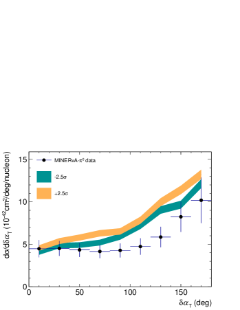
   Figure 5: Effect of varying $S_{\lambda}^{\pi^{0}}$ by $\pm 2.5~{}\sigma$ compared to the MINERvA-$\pi^{0}$ measurement. Each band’s width indicates the genie prediction’s statistical uncertainty from $10^{5}$ events.

2. The relative probability of each rescattering type can be adjusted by a scale factor. There are four rescattering types for both nucleons and pions available for tuning. They are charge exchange (CEX), inelastic scattering (INEL), absorption (ABS), and pion production (PIPD). The default energy-dependent probability distributions come from hadron data tuning [54, 55, 56, 57, 58] and can be adjusted by respective scaling factors, like $S_{\textrm{CEX}}^{\pi}$ for CEX of all pions, listed in Table 4. The relative probabilities of all four rescattering type will be normalized such that they sum up to one. Scaling factors directly multiply the probability of each type, with new relative probabilities subsequently renormalized. More specifically, suppose the initial fraction of absorption, $f_{\textrm{ABS}}$, is $0.5$, which means that the sum of the other fractions is $f_{\textrm{other}}=f_{\textrm{INEL}}+f_{\textrm{CEX}}+f_{\textrm{PIPD}}=1-0.5=0.5$. If $f_{\textrm{ABS}}$ is scaled up with $S_{\textrm{ABS}}=2$, the new absorption fraction is

   $$f^{\prime}_{\textrm{ABS}}=\frac{f_{\textrm{ABS}}*S_{\textrm{ABS}}}{f_{\textrm{ABS}}*S_{\textrm{ABS}}+f_{\textrm{oth}}}=2/3,$$ (3)

   which is not equal to simply multiplying $f_{\textrm{ABS}}$ by $S_{\textrm{ABS}}$ due to the presence of the other rescattering types. Hence, it is unavoidable that a change of the scaling factor for one type would affect others. Nonetheless, when the cross section is plotted with a breakdown according to rescattering type, interpretation will be clear regarding the increase or decrease of a particular FSI type. This correlation implies that the scaling parameters’ effective impact on FSI fate is often less pronounced than what the raw numbers suggest. As illustrated in the above example, $f_{\textrm{ABS}}$ is only scaled up by $f^{\prime}_{\textrm{ABS}}/f_{\textrm{ABS}}=4/3=1.3$ instead of $S_{\textrm{ABS}}=2$. Hence, a relatively more relaxed Gaussian prior, with a $\sigma$ of $0.5$, is placed on the FSI fate scales, slightly larger than the systematic uncertainties shown in Table 4.

   Understanding each rescattering type is crucial for interpreting tuning results. A detailed elaboration of the four tunable FSI types is given as follows.

   1. CEX involves changing the charge of the participating particles; for example,

      $$\pi^{+}+\textrm{n}\rightarrow\pi^{0}+\textrm{p},$$ (4)

      or vice versa. This rescattering type is crucial for event topologies requiring the presence of a pion; depending on the signal pion charge, CEX could migrate events between signal and background.

   2. INEL is the case where the nucleus is left in an excited state after the rescattering. This category only contains the situation where a single additional nucleon is emitted/knocked-out after rescattering. Since it does not affect the number of pions produced, it will not convert an event from a pion-less topology to a pion-production topology. The effects on nucleons are two-fold. Firstly, it can alter the number of signal events within each event topology. If the inelastic rescattering leads to two low-momentum protons below the detection threshold as opposed to a high-momentum proton, this signal event will be discarded as no protons are observed. Secondly, INEL invariably changes the kinematics of the rescattering particle. Be it the leading proton or the leading pion, based on which the TKI observables are calculated, the TKI distribution shape will be affected. Hence, while $S_{\textrm{INEL}}^{\textrm{N}}$ would affect all four data sets, $S_{\textrm{INEL}}^{\pi}$ would only affect T2K-$\pi^{+}$ and MINERvA-$\pi^{0}$.

   3. ABS refers to the case where the particle undergoes an interaction so that it does not emerge as a final particle. For example, $\pi^{+}$ can interact with two or more nucleons, initially forming a baryon resonance that subsequently interacts with other nucleons, emitting multiple nucleons rather than pions. Hence, the $\pi^{+}$ would not emerge from the nucleus anymore.

   4. PIPD happens for energetic particles where an extra pion emerges as a result of the rescattering, such as

      $$\textrm{p}+\textrm{p}\rightarrow\textrm{p}+\textrm{n}+\pi^{+}.$$ (5)

      Such an interaction significantly alters the event topology.

IV The First TKI-Driven GENIE Tunes

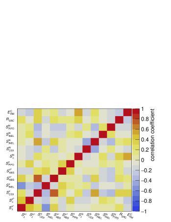
Figure 6: Correlation coefficient for AllPar on Combi-26.

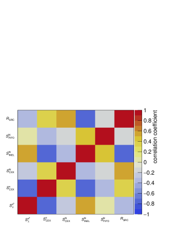
Figure 7: Similar to Fig. 6 but for RedPar.

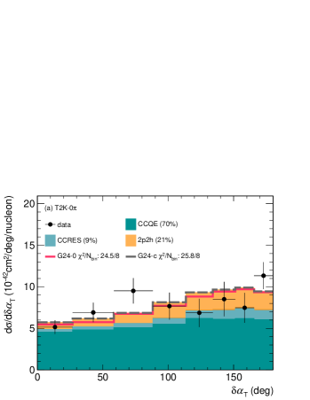
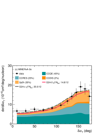
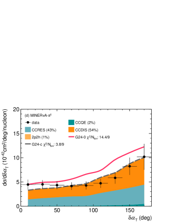
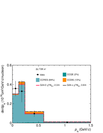
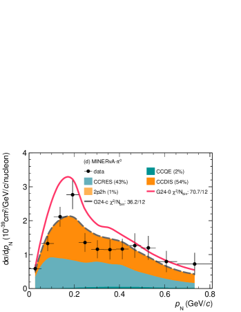
Figure 8: Similar to Fig. 2 but with G24-c. The nominal tune, G24-0, is also plotted for comparison.

Figure 9: Similar to Fig. 9 but for the $p_{\textrm{N}}$ ($\delta p_{\textrm{T}}$ for T2K-$0\pi$) measurements.

Given the intricate correlations among model parameters, determining which ones are most sensitive to the data proves challenging. Considerable correlation and anti-correlation are observed between different FSI fates for the same particle, e.g. $S_{\textrm{ABS}}^{\pi^{\pm}}$ and $S_{\textrm{CEX}}^{\pi}$, as shown in Figs. 6 and 7. Our tuning began with the AllPar parameter set, achieving the best result with Combi-15, which is denoted as Combi-Best-AllPar in Table 3 (cf. Fig. 4 for the $\chi^{2}$ distribution of all combinations). Observations showed that for most combinations, certain parameters remained close to their default values, within $1$ $\sigma$ of the imposed priors, such as $S_{\textrm{PIPD}}^{\pi}$ since none of the data sets has a significant contribution from PIPD of pions—Removing these parameters from the tuning process does not significantly affect the outcome. Therefore, we then constructed a reduced set comprising only $R_{\textrm{SRC}}$, $S_{\lambda}^{\pi^{0}}$, $S_{\textrm{CEX}}^{\pi}$, $S_{\textrm{CEX}}^{\textrm{N}}$, $S_{\textrm{ABS}}^{\textrm{N}}$, and $S_{\textrm{PIPD}}^{\textrm{N}}$ (denoted as RedPar in Table 4) and ran the tuning on the 26 combinations with it. Note that the parameters most correlated with $S_{\textrm{CEX}}^{\pi}$ and $S_{\lambda}^{\pi^{0}}$ are not present in RedPar. The RedPar tuning proved more stable, with nearly all combinations showing a more negative $\chi^{2}$ change than the AllPar tuning as shown in Fig. 4. Moreover, the single-observable (Combi-1 to 5), single-measurement (Combi-6 to 9), single-experiment (Combi-10 and 11), and single-topology (Combi-12 and 13) combinations all systematically yielded no or very limited overall (tuned plus validation) improvement post-tuning. The best tuning then occurred with Combi-26 (Combi-Best-RedPar in Table 3), that is, all TKI variables excluding $\delta\phi_{\textrm{T}}$ and $\delta p_{\textrm{T}}$ (unless no $p_{\textrm{N}}$ is available)—$\delta\alpha_{\textrm{T}}$, $p_{\textrm{N}}$ (or $\delta p_{\textrm{T}}$ if $p_{\textrm{N}}$ is unavailable), and $\delta p_{\textrm{TT}}$—from pionless and pion-production measurements in both T2K and MINERvA.

Table 5 summarizes the primary results of our tuning process. The tuned RedPar, G24_20i_06_22c (G24-c), is derived from the observable set Combi-Best-RedPar, and the tuned AllPar, G24_20i_fullpara_alt (G24-t), is from Combi-Best-AllPar. The upper part of Table 5 contains the parameter values. For the G24-c tune, changes to the SF-LFG model were moderately sized ($R_{\textrm{SRC}}$ increases from $0.12$ to $0.15$), while in the hA model, $S_{\lambda}^{\pi^{0}}$ and $S_{\textrm{CEX}}^{\pi}$ are highly suppressed and the nucleon FSI has larger CEX and PIPD and lower ABS. The tune G24-t differs most significantly from G24-c in $R_{\textrm{SRC}}$ and $S_{\textrm{CEX}}^{\pi}$. The table’s lower section illustrates $\chi^{2}$ improvements for selected observables and their corresponding validation sets. Crucially, tuning should also enhance the accuracy of validation set descriptions. Overall, both tunes have substantial reduction in the total $\chi^{2}$. In the following, we will discuss the two tunes.

Parameter	Nominal (G24-0)	RedPar (G24-c)	AllPar (G24-t)
SF-LFG
$R_{\textrm{SRC}}$	0.12	0.15 $\pm$ 0.08	0.30 $\pm$ 0.05
$E_{\textrm{RM}}^{\textrm{C}}$	0.01	0.01	0.011 $\pm$ 0.003
hA
$S_{\lambda}^{\pi^{\pm}}$	$1.0\pm 0.2$	1.0	1.11 $\pm$ 0.16
$S_{\lambda}^{\pi^{0}}$	$1.0\pm 0.2$	0.22 $\pm$ 0.07	0.17 $\pm$ 0.06
$S_{\lambda}^{\textrm{N}}$	$1.0\pm 0.2$	1.0	1.20 $\pm$ 0.12
$S_{\textrm{CEX}}^{\pi}$	$1.0\pm 0.5$	0.26 $\pm$ 0.12	1.53 $\pm$ 0.37
$S_{\textrm{CEX}}^{\textrm{N}}$	$1.0\pm 0.4$	1.43 $\pm$ 0.34	1.41 $\pm$ 0.38
$S_{\textrm{INEL}}^{\pi}$	$1.0\pm 0.4$	1.0	0.67 $\pm$ 0.30
$S_{\textrm{INEL}}^{\textrm{N}}$	$1.0\pm 0.4$	1.0	1.26 $\pm$ 0.48
$S_{\textrm{ABS}}^{\pi^{\pm}}$	$1.0\pm 0.2$	1.0	1.59 $\pm$ 0.31
$S_{\textrm{ABS}}^{\pi^{0}}$	$1.0\pm 0.2$	1.0	0.90 $\pm$ 0.28
$S_{\textrm{ABS}}^{\textrm{N}}$	$1.0\pm 0.2$	0.25 $\pm$ 0.28	0.28 $\pm$ 0.27
$S_{\textrm{PIPD}}^{\pi}$	$1.0\pm 0.2$	1.0	1.12 $\pm$ 0.30
$S_{\textrm{PIPD}}^{\textrm{N}}$	$1.0\pm 0.2$	2.05 $\pm$ 0.48	1.27 $\pm$ 0.48
combi
untuned		231.75	161.26
tuned		174.84	122.53
diff		-56.91	-38.73
vald
untuned		229.5	299.99
tuned		214.7	263.41
diff		-14.8	-36.58
combi+vald
untuned		461.25	461.25
tuned		389.54	385.94
diff		-71.71	-75.31

Table 5: Parameters in G24-0, G24-c, and G24-t. Those without errors are not tuned. Lower section: combi indicates that the following $\chi^{2}$ sums are calculated for the tuned measurements (i.e. Combi-Best-RedPar and Combi-Best-AllPar for G24-c and G24-t, respectively), while vald indicates that the respective validation sets are used; untuned means that the $\chi^{2}$ calculation uses the nominal values of the parameters, while tuned denotes the tuned ones. diff displays the improvement achieved by the respective tuning.

IV.1 Reduced Tune: G24-c

To assess the tune’s quality, we plot predictions using G24-c for $\delta\alpha_{\textrm{T}}$ and $p_{\textrm{N}}$ in Figs. 9 and 9, respectively. For T2K-$0\pi$, T2K-$\pi^{+}$ and MINERvA-$0\pi$, the new $\chi^{2}$ values are comparable to those obtained with G24-0, changing less than the number of bins. For MINERvA-$\pi^{0}$, G24-c is distinctly better than G24-0, thereby demonstrating the possibility of simultaneous good descriptions of both pion-less and pion production samples with constrained parameters from cross-topology TKI tuning.

Examining individual datasets closely helps to understand the origin of the improvement. The decomposition of the cross section for $\delta\alpha_{\textrm{T}}$ according to the FSI fates of the $\pi^{0}$ is presented in Fig. 10. The hA model rescatters primary interaction products only once, and records this event with a rescattering code for these particles. The rescattered products, which are the final outputs, are stored as daughters of the primary interaction products. Hence, the FSI fate that produces the final products can be checked by the rescattering code of their first parent. More specifically, we loop through all final-state particles to look for the leading $\pi^{0}$ and check the rescattering code of its first parent.

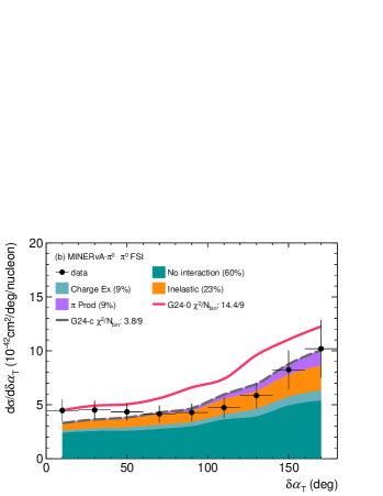
Figure 10: MINERvA-$\pi^{0}$ $\delta\alpha_{\textrm{T}}$ measurement compared to genie predictions decomposed in $\pi^{0}$ FSI fates with (a) G24-0 and (b) G24-c.

In MINERvA-$\pi^{0}$, the number of $\pi^{0}$s undergoing no FSI (“No Interaction” as shown in the figures) is adjustable via the $S_{\lambda}^{\pi^{0}}$ parameter. A decrease in $S_{\lambda}^{\pi^{0}}$ reduces the size of the “No Interaction” events, as is shown in Fig. 10b when compared to Fig. 10a. Meanwhile, an increase in $\pi^{0}$ rescattering only manifests in pion-less measurements through ABS. There is indeed an increase of ABS for $\pi^{0}$ in T2K-$0\pi$ and MINERvA-$0\pi$, but the fraction is small to begin with, so the impact is small. The increase of $\pi^{0}$ rescattering can increase T2K-$\pi^{+}$ via CEX as discussed below. However, due to the significant suppression of CEX, its impact on T2K-$\pi^{+}$ is also minimal (for detailed breakdown, see Figs. 14-16 in Appendix .2).

As shown in Fig. 10a, the MINERvA-$\pi^{0}$ prediction from the nominal tune has considerable contributions from CEX controlled by $S_{\textrm{CEX}}^{\pi}$. It does not impact T2K-$0\pi$ and MINERvA-$0\pi$ as CEX only changes the pion type without removing them. Hence, events with pions in the final state would be rejected in these two data sets regardless of the pion charge. In principle, CEX will also migrate events between the signal and background definitions for T2K-$\pi^{+}$ when a $\pi^{0}$ is converted to a $\pi^{+}$ and vice verse. However, T2K-$\pi^{+}$ does not have a considerable CEX fraction to begin with, so changing CEX will have a minimal impact on its prediction. Hence, this is one of the most effective paths to decrease the MINERvA-$\pi^{0}$ cross section prediction without affecting other measurements, and indeed the $S_{\textrm{CEX}}^{\pi}$ is heavily suppressed as shown in Table 5 and illustrated in Fig. 10b compared to Fig. 10a. However, due to the intricate correlation between the FSI fates in the hA implementation discussed in Sec. III.2, although $S_{\textrm{INEL}}^{\pi}$ and $S_{\textrm{PIPD}}^{\pi}$ are not modified explicitly, a considerable increase is observed in both INEL and PIPD for MINERvA-$\pi^{0}$.

Suppressing both “No Interaction” and CEX for $\pi^{0}$ adjusts the MINERvA-$\pi^{0}$ prediction to the appropriate magnitude with small impacts on other data sets. The effects of the other parameter changes are more transparent in the comparison of the $p_{\textrm{N}}$ distribution of MINERvA-$\pi^{0}$ between Figs. 11a and 11b. A relatively large increase in $S_{\textrm{CEX}}^{\textrm{N}}$ and $S_{\textrm{PIPD}}^{\textrm{N}}$ moves events away from the Fermi motion peak at $p_{\textrm{N}}\leq 0.25~{}\textrm{GeV}/c$; the same effect can be achieved by an increased $R_{\textrm{SRC}}$.

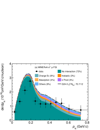
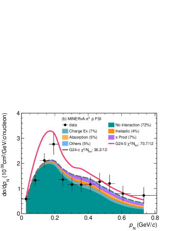
Figure 11: Similar to Fig. 10 but for $p_{\textrm{N}}$ with proton FSI fate decomposition. Note that the “Absorption” of the proton is referring to the absorption of the $\pi^{+}$ from the decay of $\Delta^{++}$, which could lead to emission of nucleons as discussed in Sec. III.2.

IV.2 Alternative Tune: G24-t

A similar improvement is achieved by the intermediate tune, G24-t, illustrated in Fig. 12. Instead of significantly increasing proton PIPD to elevate the $p_{\textrm{N}}$ tail, this tune notably enhances $R_{\textrm{SRC}}$—less-energetic final states are present and therefore an increased RES/DIS (Fig. 12a) ratio. Rather than suppressing $S_{\textrm{CEX}}^{\pi}$ (cf. Fig. 16d in Appendix .2), this tune significantly increases it (Fig. 12b) to offset the further reduction of “No Interaction” $\pi^{0}$ events (smaller $S_{\lambda}^{\pi^{0}}$ in AllPar, cf. Table 5). Overall, this leads to a reduction of $75.31$ in $\chi^{2}$ (Table 5), similar to G24-c, as well as a good data-MC agreement across all data sets.

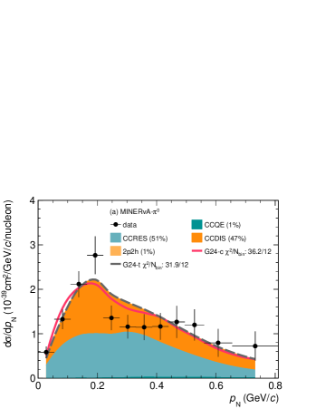
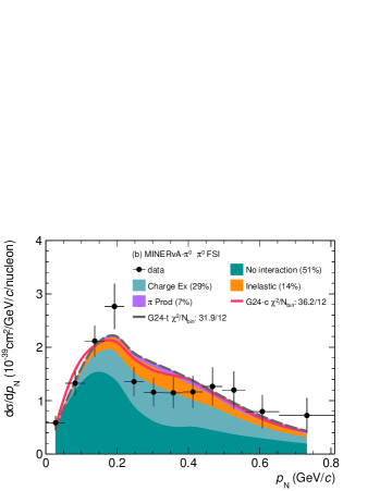
Figure 12: MINERvA-$\pi^{0}$ $p_{\textrm{N}}$ measurement compared to genie predictions decomposed in (a) $\nu$-N interaction, (b) $\pi^{0}$ FSI, and (c) proton FSI for the alternative tune, G24-t.

V Summary and Outlook

This work represents the first global tuning effort on TKI data. Our partial tune of the SF-LFG and hA models, G24_20i_06_22c (G24-c), provides an effective theory to better describe both the neutrino-hydrocarbon pionless and pion production. The largest change in the model is demanded by the MINERvA-$\pi^{0}$ TKI measurement [12] that was significantly overestimated in genie. The improvement is crucial for future accelerator-based neutrino experiments. This tuning configuration has been integrated into the master branch of genie and is slated for inclusion in the upcoming release.

To develop an effective theory, we focused on the most sensitive parameters, $R_{\textrm{SRC}}$, $S_{\lambda}^{\pi^{0}}$, $S_{\textrm{CEX}}^{\pi}$, $S_{\textrm{CEX}}^{\textrm{N}}$, $S_{\textrm{ABS}}^{\textrm{N}}$, and $S_{\textrm{PIPD}}^{\textrm{N}}$, of the SF-LFG and hA models, reducing the total number of parameters from $14$ to $6$. The corresponding best combination of observables is $\delta\alpha_{\textrm{T}}$, $p_{\textrm{N}}$ (or $\delta p_{\textrm{T}}$ if no $p_{\textrm{N}}$ is available), and $\delta p_{\textrm{TT}}$, from pionless and pion-production measurements in both T2K and MINERvA. In doing so, the pion production model is held fixed such that the tuned values of $S_{\lambda}^{\pi^{0}}$, $S_{\textrm{CEX}}^{\pi}$, $S_{\textrm{ABS}}^{\textrm{N}}$, and $S_{\textrm{PIPD}}^{\textrm{N}}$ depart from the established constraints from hadron measurements. A different pion production model might compensate part of these model tuning effects. We also chose the hA FSI model for practical reasons. Its sequential treatment of MFP and rescattering should be considered as a numerical advantage (as was also pointed out in Ref. [9]). Other more sophisticated models could be considered in future tunes. With the existing four TKI measurements from T2K and MINERvA, we have also derived other effective tunes like G24_20i_fullpara_alt (G24-t). The degeneracy can be resolved with additional data, particularly from argon-based measurements [20, 21, 22, 23, 24, 61].

appendix

.1 Combinations of Observables

Table 6 displays the tested combinations of observables:

• Combi-$1$ through $5$ are cross-experiment selections of a single observable. For example, Combi-$3$ uses only $\delta\alpha_{\textrm{T}}$ from all four data sets. If a chosen observable is absent from a dataset, that dataset is excluded from the specific combination. For example, T2K-$0\pi$ is not used in Combi-1 due to the absence of $p_{\textrm{N}}$.

• Combi-$6$ through $9$ incorporate all variables from a single measurement. For example, Combi-$9$ uses MINERvA-$\pi^{0}$ only.

• Combi-$10$ to $13$ uses two out of four measurements according to the experiment or topology. For example, Combi-$10$ uses only the two data sets from T2K, and Combi-$13$ only with pion production.

• Combi-14 to 17 combine two separate combinations:

  Combi-14 $$=\texttt{Combi-3}\cup\texttt{Combi-5},$$

  Combi-15 $$=\texttt{Combi-1}\cup\texttt{Combi-2},$$

  Combi-16 $$=\texttt{Combi-1}\cup\texttt{Combi-3},$$

  Combi-17 $$=\texttt{Combi-2}\cup\texttt{Combi-3}.$$

• Combi-18 through 22 result from merging three combinations:

  Combi-18 $$=\texttt{Combi-1}\cup\texttt{Combi-3}\cup\texttt{Combi-5},$$

  Combi-19 $$=\texttt{Combi-2}\cup\texttt{Combi-3}\cup\texttt{Combi-5},$$

  Combi-20 $$=\texttt{Combi-3}\cup\texttt{Combi-4}\cup\texttt{Combi-5},$$

  Combi-21 $$=\texttt{Combi-1}\cup\texttt{Combi-2}\cup\texttt{Combi-3},$$

  Combi-22 $$=\texttt{Combi-1}\cup\texttt{Combi-2}\cup\texttt{Combi-4}.$$

• Combi-23 merges four different combinations:

  Combi-23 $$=\texttt{Combi-1}\cup\texttt{Combi-2}\cup$$

  $$\texttt{Combi-3}\cup\texttt{Combi-5}.$$

• Combi-24 encompasses all variables, acting as the superset.

• Combi-$25$ and $26$ are the same as Combi-$21$ and $23$, respectively, except that $\delta p_{\textrm{T}}$ in MINERvA-$0\pi$ is removed to avoid correlation with $p_{\textrm{N}}$ in the same data set.

Figure 4 shows the change in $\chi^{2}$ for the complete observable set (tuned plus validation) as a function of the tuning combination, where the two model parameter sets, AllPar and RedPar, are compared and it can be seen that the respective minima happen at Combi-15 and 26.

.2 $\pi^{0}$ FSI Fate Decomposition for G24-0 and G24-c

Figures 14-16 display comparisons of G24-0 and G24-c predictions to data, detailing the composition by $\pi^{0}$ FSI fate.

Combi-	1	2	3	4	5	6	7	8	9	10	11	12	13	14	15 (Best- AllPar)	16	17	18	19	20	21	22	23	24 (Super- set)	25	26 (Best- RedPar)
T2K-$0\pi$
$\delta\alpha_{\textrm{T}}$			$\checkmark$			$\checkmark$				$\checkmark$		$\checkmark$		$\checkmark$		$\checkmark$	$\checkmark$	$\checkmark$	$\checkmark$	$\checkmark$	$\checkmark$		$\checkmark$	$\checkmark$	$\checkmark$	$\checkmark$
$\delta p_{\textrm{T}}$		$\checkmark$				$\checkmark$				$\checkmark$		$\checkmark$			$\checkmark$		$\checkmark$		$\checkmark$		$\checkmark$	$\checkmark$	$\checkmark$	$\checkmark$	$\checkmark$	$\checkmark$
$\delta\phi_{\textrm{T}}$				$\checkmark$		$\checkmark$				$\checkmark$		$\checkmark$								$\checkmark$		$\checkmark$		$\checkmark$
T2K-$\pi^{+}$
$\delta\alpha_{\textrm{T}}$			$\checkmark$				$\checkmark$			$\checkmark$			$\checkmark$	$\checkmark$		$\checkmark$	$\checkmark$	$\checkmark$	$\checkmark$	$\checkmark$	$\checkmark$		$\checkmark$	$\checkmark$	$\checkmark$	$\checkmark$
$p_{\textrm{N}}$	$\checkmark$						$\checkmark$			$\checkmark$			$\checkmark$		$\checkmark$	$\checkmark$		$\checkmark$			$\checkmark$	$\checkmark$	$\checkmark$	$\checkmark$	$\checkmark$	$\checkmark$
$\delta p_{\textrm{TT}}$					$\checkmark$		$\checkmark$			$\checkmark$			$\checkmark$	$\checkmark$				$\checkmark$	$\checkmark$	$\checkmark$			$\checkmark$	$\checkmark$		$\checkmark$
MINERvA-$0\pi$
$\delta\alpha_{\textrm{T}}$			$\checkmark$					$\checkmark$			$\checkmark$	$\checkmark$		$\checkmark$		$\checkmark$	$\checkmark$	$\checkmark$	$\checkmark$	$\checkmark$	$\checkmark$		$\checkmark$	$\checkmark$	$\checkmark$	$\checkmark$
$p_{\textrm{N}}$	$\checkmark$							$\checkmark$			$\checkmark$	$\checkmark$			$\checkmark$	$\checkmark$		$\checkmark$			$\checkmark$	$\checkmark$	$\checkmark$	$\checkmark$	$\checkmark$	$\checkmark$
$\delta p_{\textrm{T}}$		$\checkmark$						$\checkmark$			$\checkmark$	$\checkmark$			$\checkmark$		$\checkmark$		$\checkmark$		$\checkmark$	$\checkmark$	$\checkmark$	$\checkmark$
$\delta\phi_{\textrm{T}}$				$\checkmark$				$\checkmark$			$\checkmark$	$\checkmark$								$\checkmark$		$\checkmark$		$\checkmark$
MINERvA-$\pi^{0}$
$\delta\alpha_{\textrm{T}}$			$\checkmark$						$\checkmark$		$\checkmark$		$\checkmark$	$\checkmark$		$\checkmark$	$\checkmark$	$\checkmark$	$\checkmark$	$\checkmark$	$\checkmark$		$\checkmark$	$\checkmark$	$\checkmark$	$\checkmark$
$p_{\textrm{N}}$	$\checkmark$								$\checkmark$		$\checkmark$		$\checkmark$		$\checkmark$	$\checkmark$		$\checkmark$			$\checkmark$	$\checkmark$	$\checkmark$	$\checkmark$	$\checkmark$	$\checkmark$
$\delta p_{\textrm{TT}}$					$\checkmark$				$\checkmark$		$\checkmark$		$\checkmark$	$\checkmark$				$\checkmark$	$\checkmark$	$\checkmark$			$\checkmark$	$\checkmark$		$\checkmark$

Table 6: Specifications of observable combinations within the tuning superset in Table 3.

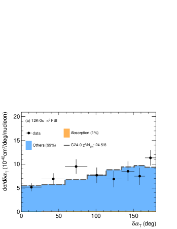
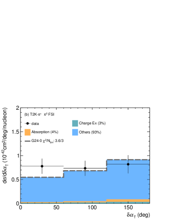
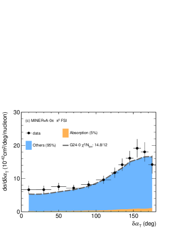
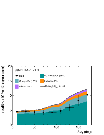
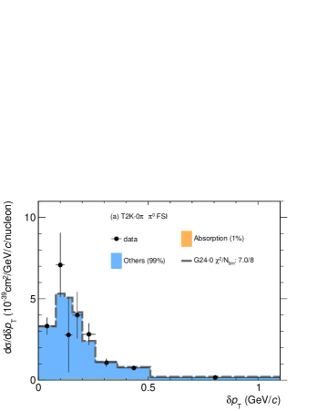
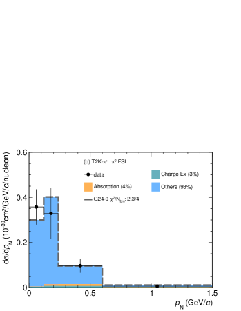
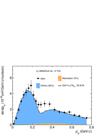
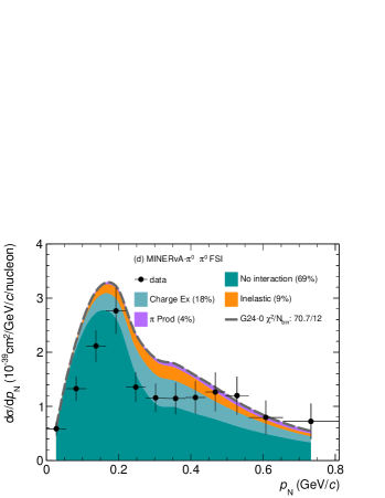
Figure 13: Extension of Fig. 10a to all four $\delta\alpha_{\textrm{T}}$ measurements.

Figure 14: Extension of Fig. 10a but to all four $p_{\textrm{N}}$ measurements.

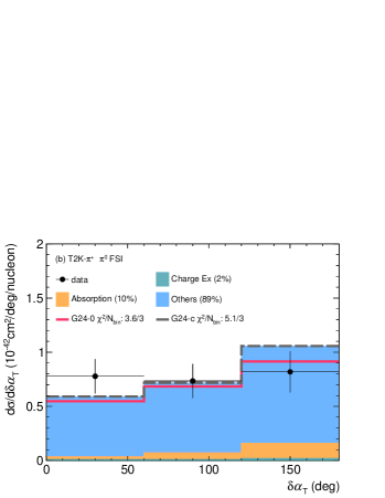
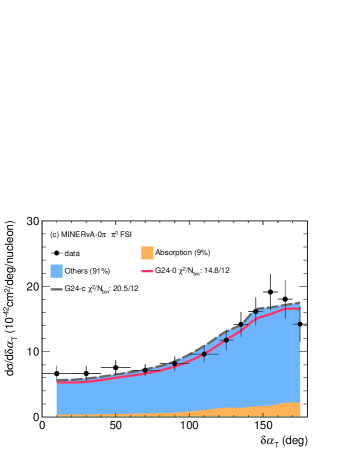
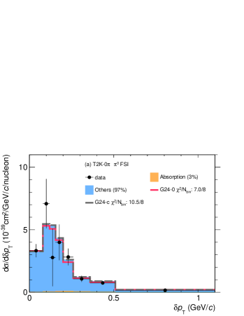
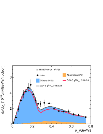
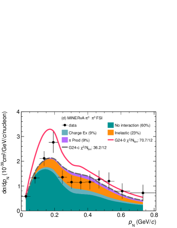
Figure 15: Extension of Fig. 10b to all four $\delta\alpha_{\textrm{T}}$ measurements.

Figure 16: Extension of Fig. 10b but to all four $p_{\textrm{N}}$ measurements.

References

- Abe et al. [2018a] K. Abe et al. (Hyper-Kamiokande), (2018a), arXiv:1805.04163 [physics.ins-det] .
- Acciarri et al. [2016a] R. Acciarri et al. (DUNE), (2016a), arXiv:1601.05471 [physics.ins-det] .
- Acciarri et al. [2015a] R. Acciarri et al. (DUNE), (2015a), arXiv:1512.06148 [physics.ins-det] .
- Strait et al. [2016] J. Strait et al. (DUNE), (2016), arXiv:1601.05823 [physics.ins-det] .
- Acciarri et al. [2016b] R. Acciarri et al. (DUNE), (2016b), arXiv:1601.02984 [physics.ins-det] .
- Andreopoulos et al. [2010] C. Andreopoulos et al., Nucl. Instrum. Meth. A 614, 87 (2010), arXiv:0905.2517 [hep-ph] .
- Tena-Vidal et al. [2021] J. Tena-Vidal et al. (GENIE), Phys. Rev. D 104, 072009 (2021), arXiv:2104.09179 [hep-ph] .
- Tena-Vidal et al. [2022a] J. Tena-Vidal et al. (GENIE), Phys. Rev. D 105, 012009 (2022a), arXiv:2106.05884 [hep-ph] .
- Tena-Vidal et al. [2022b] J. Tena-Vidal et al. (GENIE), Phys. Rev. D 106, 112001 (2022b), arXiv:2206.11050 [hep-ph] .
- Lu et al. [2015] X.-G. Lu, D. Coplowe, R. Shah, G. Barr, D. Wark, and A. Weber, Phys. Rev. D 92, 051302 (2015), arXiv:1507.00967 [hep-ex] .
- Lu et al. [2016] X.-G. Lu, L. Pickering, S. Dolan, G. Barr, D. Coplowe, Y. Uchida, D. Wark, M. O. Wascko, A. Weber, and T. Yuan, Phys. Rev. C94, 015503 (2016), arXiv:1512.05748 [nucl-th] .
- Coplowe et al. [2020] D. Coplowe et al. (MINERvA), Phys. Rev. D 102, 072007 (2020), arXiv:2002.05812 [hep-ex] .
- Furmanski and Sobczyk [2017] A. P. Furmanski and J. T. Sobczyk, Phys. Rev. C 95, 065501 (2017), arXiv:1609.03530 [hep-ex] .
- Lu and Sobczyk [2019] X.-G. Lu and J. T. Sobczyk, Phys. Rev. C 99, 055504 (2019), arXiv:1901.06411 [hep-ph] .
- Cai et al. [2019] T. Cai, X.-G. Lu, and D. Ruterbories, Phys. Rev. D 100, 073010 (2019), arXiv:1907.11212 [hep-ex] .
- Abe et al. [2018b] K. Abe et al. (T2K), Phys. Rev. D 98, 032003 (2018b), arXiv:1802.05078 [hep-ex] .
- Abe et al. [2021] K. Abe et al. (T2K), Phys. Rev. D 103, 112009 (2021), arXiv:2102.03346 [hep-ex] .
- Lu et al. [2018] X.-G. Lu et al. (MINERvA), Phys. Rev. Lett. 121, 022504 (2018), arXiv:1805.05486 [hep-ex] .
- Cai et al. [2020] T. Cai et al. (MINERvA), Phys. Rev. D 101, 092001 (2020), arXiv:1910.08658 [hep-ex] .
- Abratenko et al. [2022] P. Abratenko et al. (MicroBooNE), (2022), arXiv:2211.03734 [hep-ex] .
- Abratenko et al. [2023a] P. Abratenko et al. (MicroBooNE), Phys. Rev. D 108, 053002 (2023a), arXiv:2301.03700 [hep-ex] .
- Abratenko et al. [2023b] P. Abratenko et al. (MicroBooNE), Phys. Rev. Lett. 131, 101802 (2023b), arXiv:2301.03706 [hep-ex] .
- Abratenko et al. [2023c] P. Abratenko et al. (MicroBooNE), (2023c), arXiv:2310.06082 [nucl-ex] .
- Abratenko et al. [2024] P. Abratenko et al. (MicroBooNE), (2024), arXiv:2403.19574 [hep-ex] .
- Khachatryan et al. [2021] M. Khachatryan et al. (CLAS, e4v), Nature 599, 565 (2021).
- Yang [2023] K. Yang, Measurement of the pion charge exchange differential cross section on Argon with the ProtoDUNE-SP detector, Ph.D. thesis, Oxford University, Oxford U. FERMILAB-THESIS-2023-19. (2023).
- Hamacher-Baumann et al. [2020] P. Hamacher-Baumann, X.-G. Lu, and J. Martín-Albo, Phys. Rev. D 102, 033005 (2020), arXiv:2005.05252 [physics.ins-det] .
- Dolan [2018] S. Dolan, (2018), arXiv:1810.06043 [hep-ex] .
- Bourguille et al. [2021] B. Bourguille, J. Nieves, and F. Sánchez, JHEP 04, 004 (2021), arXiv:2012.12653 [hep-ph] .
- Franco-Patino et al. [2021] J. M. Franco-Patino, M. B. Barbaro, J. A. Caballero, and G. D. Megias, Phys. Rev. D 104, 073008 (2021), arXiv:2106.02311 [nucl-th] .
- Ershova et al. [2022] A. Ershova et al., Phys. Rev. D 106, 032009 (2022), arXiv:2202.10402 [hep-ph] .
- Franco-Patino et al. [2022] J. M. Franco-Patino, R. González-Jiménez, S. Dolan, M. B. Barbaro, J. A. Caballero, G. D. Megias, and J. M. Udias, Phys. Rev. D 106, 113005 (2022), arXiv:2207.02086 [nucl-th] .
- Chakrani et al. [2023] J. Chakrani et al., (2023), arXiv:2308.01838 [hep-ex] .
- Ershova et al. [2023] A. Ershova et al., Phys. Rev. D 108, 112008 (2023), arXiv:2309.05410 [hep-ph] .
- Munteanu [2022] L. Munteanu, “Modeling neutrino-nucleus interaction uncertainties for dune long-baseline sensitivity studies,” (2022), nuInt, Seoul, KOREA, [Conference presentation].
- Munteanu [2023] L. Munteanu, “Genie generator,” (2023), commit SHA:64135ac.
- Alvarez-Ruso et al. [2021] L. Alvarez-Ruso et al. (GENIE), Eur. Phys. J. ST 230, 4449 (2021), arXiv:2106.09381 [hep-ph] .
- Hill and Paz [2010] R. J. Hill and G. Paz, Phys. Rev. D 82, 113005 (2010), arXiv:1008.4619 [hep-ph] .
- Nieves et al. [2004] J. Nieves, J. E. Amaro, and M. Valverde, Phys. Rev. C 70, 055503 (2004), [Erratum: Phys.Rev.C 72, 019902 (2005)], arXiv:nucl-th/0408005 .
- Nieves et al. [2011] J. Nieves, I. Ruiz Simo, and M. J. Vicente Vacas, Phys. Rev. C 83, 045501 (2011), arXiv:1102.2777 [hep-ph] .
- Gonzaléz-Jiménez et al. [2014] R. Gonzaléz-Jiménez, G. D. Megias, M. B. Barbaro, J. A. Caballero, and T. W. Donnelly, Phys. Rev. C 90, 035501 (2014), arXiv:1407.8346 [nucl-th] .
- Pais [1971] A. Pais, Annals Phys. 63, 361 (1971).
- Kovalenko [1990] S. G. Kovalenko, Sov. J. Nucl. Phys. 52, 934 (1990).
- Berger and Sehgal [2007] C. Berger and L. M. Sehgal, Phys. Rev. D 76, 113004 (2007), arXiv:0709.4378 [hep-ph] .
- Bodek and Yang [2002] A. Bodek and U. K. Yang, Nucl. Phys. B Proc. Suppl. 112, 70 (2002), arXiv:hep-ex/0203009 .
- Aivazis et al. [1991] M. A. G. Aivazis, W.-K. Tung, and F. I. Olness, in Particles & Fields 91: Meeting of the Division of Particles & Fields of the APS (1991) pp. 0663–665, arXiv:hep-ph/9302305 .
- Berger and Sehgal [2009] C. Berger and L. M. Sehgal, Phys. Rev. D 79, 053003 (2009), arXiv:0812.2653 [hep-ph] .
- Yang et al. [2009] T. Yang, C. Andreopoulos, H. Gallagher, K. Hoffmann, and P. Kehayias, Eur. Phys. J. C 63, 1 (2009), arXiv:0904.4043 [hep-ph] .
- Andreopoulos et al. [2015] C. Andreopoulos, C. Barry, S. Dytman, H. Gallagher, T. Golan, R. Hatcher, G. Perdue, and J. Yarba, (2015), arXiv:1510.05494 [hep-ph] .
- Buckley et al. [2010] A. Buckley, H. Hoeth, H. Lacker, H. Schulz, and J. E. von Seggern, Eur. Phys. J. C 65, 331 (2010), arXiv:0907.2973 [hep-ph] .
- D’Agostini [1994] G. D’Agostini, Nucl. Instrum. Meth. A 346, 306 (1994).
- Hanson et al. [2005] K. M. Hanson, T. Kawano, and P. Talou, AIP Conf. Proc. 769, 304 (2005).
- Frühwirth, R. et al. [2012] Frühwirth, R., Neudecker, D., and Leeb, H., EPJ Web of Conferences 27, 00008 (2012).
- Rowntree et al. [1999] D. Rowntree et al. (LADS), Phys. Rev. C 60, 054610 (1999).
- Navon et al. [1983] I. Navon, D. Ashery, J. Alster, G. Azuelos, B. M. Barnett, W. Gyles, R. R. Johnson, D. R. Gill, and T. G. Masterson, Phys. Rev. C 28, 2548 (1983).
- Carroll et al. [1976] A. S. Carroll, I. H. Chiang, C. B. Dover, T. F. Kycia, K. K. Li, P. O. Mazur, D. N. Michael, P. M. Mockett, D. C. Rahm, and R. Rubinstein, Phys. Rev. C 14, 635 (1976).
- Clough et al. [1974] A. S. Clough et al., Nucl. Phys. B 76, 15 (1974).
- Bauhoff [1986] W. Bauhoff, Atomic Data and Nuclear Data Tables 35, 429 (1986).
- Mashnik et al. [2000] S. G. Mashnik, R. J. Peterson, A. J. Sierk, and M. R. Braunstein, Phys. Rev. C 61, 034601 (2000).
- Ishibashi et al. [1997] K. Ishibashi et al., J. Nucl. Sci. Technol. 34, 529 (1997).
- Acciarri et al. [2015b] R. Acciarri et al. (MicroBooNE, LAr1-ND, ICARUS-WA104), (2015b), arXiv:1503.01520 [physics.ins-det] .