A modified Polak-Ribière-Polyak type conjugate gradient method with two stepsize strategies for vector optimization
1School of Mathematics and statistics, Southwest University, Chongqing 400715, China
Abstract.
In this paper, in order to find critical points of vector-valued functions with respect to the partial order induced by a closed, convex, and pointed cone with nonempty interior, we propose a nonlinear modified Polak-Ribière-Polyak type conjugate gradient method with a nonnegative conjugate parameter. We show that the search direction in our method satisfies the sufficient descent condition independent of any line search. Furthermore, under mild assumptions, we obtain the results of global convergence with the standard Wolfe line search conditions as well as the standard Armijo line search strategy without convexity assumption of the objective functions. Computational experiments are given to show the effectiveness of the proposed method.
Keywords. Vector optimization; Conjugate gradient direction; Line search strategy; Pareto critical point
1. Introduction
Let us first consider the single-objective problem
| (1.1) |
where is continuously differentiable. The most classic first-order method to solve this problem is the steepest descent method, while the most widely used second-order method is the Newton’s method. And the conjugate gradient method proposed in [1] is one of the most commonly used and effective optimization methods between the steepest descent method and the Newton’s method, which has the characteristics of fast convergence rate, lower memory requirement and less computation cost, and has important applications in both linear and nonlinear optimization. Formally, the conjugate gradient method generates a sequence given by
| (1.2) |
where the stepsize is obtained by a line search strategy and the search direction is defined by
| (1.3) |
where is a scalar algorithmic parameter. For nonquadratic functions, Different choices for the conjugate parameter in (1.3) result in different algorithms, known as nonlinear conjugate gradient methods. Although too many to name, some notable choices would include:
where and denotes the usual inner product. We expect to get conjugate parameters that make descent directions in the sense of for all , or make meet a more stringent condition, which is called sufficient descent condition and defined as
| (1.4) |
for some and all , where denotes the Euclidian norm. A significant advantage of the FR, CD, and DY methods is that if a line search satisfying the Wolfe conditions is used, the corresponding search directions are verified to be descent. However, the PRP and HS methods do not necessarily generate descent directions even when Wolfe line searches are employed.
In this paper, we consider the following unconstrained vector optimization problem(VOP)
| (1.5) |
where is continuously differentiable, and is a pointed, closed and convex cone with nonempty interior . The partial order is given by if and only if . In vector optimization, the concept of optimality is replaced by the concept of Pareto optimality or efficiency, and we seek to find K-Pareto optimal point or K-efficient point. In practical applications, we usually take , then Problem (1.5) corresponds to the multiobjective optimization problem.
Vector optimization problems are a significant extension of multiobjective optimization, and there are a large number of real life applications of multicriteria and vectorial optimization, such as engineering design [6, 7], finance [8], machine learning [9], space exploration [10], management science [11, 12], environmental analysis and so on. Due to the wide application of vector-valued optimization, the development of strategies for solving vector-valued optimization problems has attracted wide attention. At present, a lot of research has been made in the theory and algorithm of solving vector optimization problems, and the common methods for solving vector optimization problems include scalarization approaches and descent methods. The scalarization approaches for solving vector optimization problems are to convert the original vector optimization problems into the parameterized single objective ones; see [13, 14]. The drawback of this method is that even when the original vector-valued problem has solutions, the selection of parameters may lead to unbounded numerical problems (and thus unsolvable). However, the descent methods do not require any parameter information, and thus usually perform better in numerical experiments. Many descent methods for solving scalar optimization problems have been extended to vector-valued optimization, such as projected gradient method [15, 16, 17], Newton method [18, 19, 20], steepest descent method [21, 22], proximal point method [23, 24] and so on.
In recent years, the conjugate gradient method has been extended from solving single-objective problems to solving multiobjective [25] and vector-valued problems [28, 26, 27]. The first work in this line was [28], Lucambio Pèrez and Prudente proposed a nonlinear conjugate gradient algorithm (NLCG), and generate a sequence of iterates by the following form:
| (1.6) |
where the stepsize is obtained by standard Wolfe or strong Wolfe line search strategy and the search direction is defined by
| (1.7) |
where is scalar algorithmic parameters, which are extended from the FR, CD, DY, PRP, and HS conjugate gradient algorithms for the single-objective case, and they are defined as follows
where is defined in the next section. In [28, Theorem 5.11], by assuming that the search direction is a -descent direction, Lucambio Pèrez and Prudente established the convergence result related to the PRP+ parameter given by , which remind us that the nonegativeness of parameter seems to be essential for obtaining the convergence result of the conjugate gradient method, while the nonegativeness of the PRP parameter cannot be guaranteed. To address this weakness of the PRP parameter, we extend the method considered in [29] to the vector context because the parameter of this method are nonnegative and this method show superior performance in numerical experiments. We propose a nonlinear modified Polak-Ribière-Polyak type conjugate gradient method with a nonnegative conjugate parameter, which is extended from [29], and we show that the search direction in our proposed method satisfies the sufficient descent condition no matter what stepsize strategy is adopted. Furthermore, under mild assumptions, which are natural extensions of those made for the scalar case, we obtain the results of global convergence with the standard Wolfe line search as well as the standard Armijo line search without convexity assumption of the objective functions.
The paper is organized as follows. In the next section, we present some notations, definitions and preliminary results. In Section 3, we propose the modified PRP-type conjugate gradient method and investigate some properties of this method. The global convergence of the full sequence generated by the proposed method with the standard Wolfe line search as well as the standard Armijo line search is provided in Section 4. In section 5, some numerical experiments are reported to show the ability of the proposed method. Finally, we give some concluding remarks in Section 6.
2. Preliminaries
In this section, we present the vector optimization problem studied in the present work, the first order optimality condition for it, and some notations and defnitions. Throughout this paper, let stands for the inner product in and denotes the norm, that is for . And we denote the convex hull of by , and the cone of by , let be a pointed, closed and convex cone, with nonempty interior . The partial induced by , is defined as follows
and the partial induced by , is defined as follows
A point is called a K-Pareto optimal point (or K-Pareto point) of (1.5) on , if there exists no other point , such that and . The set of the objective values of all Pareto optimal solutions is also called Pareto frontier. In turn, a point is called a K-weak Pareto optimal point (or K-weak Pareto) of (1.5) on , if there exists no other point , such that . It is clear that a Pareto optimal point is also a weak Pareto optimal point but not vice versa. Since is continuously differentiable, the subdifferential of at coincides with the Jacobian of , and is denoted by and the image of the Jacobian of at a point is denoted by . A first order optimality condition (necessary but in general not sufficient) for the problem (1.5) of a point is given by
| (2.1) |
which means that, for any , we have . A point satisfying (2.1) is called a K-Pareto critical point or a K-stationary point of problem (1.5). Note that if is not a K-Pareto critical point, then there exists a direction satisfying . This implies that is a K-descent direction for at , i.e., there exists such that for all .
The positive polar cone of is the set
| (2.2) |
since the set is closed and convex, , and thus and . According to [30, Remark 1.6], every cone in finite dimensional spaces has a closed convex bounded base if and only if it is pointed closed, which means that there is a compact set satisfying
| (2.3) |
since and , it follows that . Then
| (2.4) |
and
| (2.5) |
Remark 2.1.
It is known that , and in single-objective optimization. As for multiobjective optimization, and are the positive orthant of and we may take as the canonical basis of . If is a polyhedral cone, may be taken as a finite set of extremal rays of .
For generic which is a pointed, closed and convex cone with nonempty interior, we define
| (2.6) |
then satisfies the condition that we mentioned in (2.3).
For the convenience of the subsequent description, we define as follows
| (2.7) |
consider the compactness of , the function is well defined. Then and can be rewrite as follows
| (2.8) |
and
| (2.9) |
In the following Lemma, we will give some basic properties of the function stated in [21, Lemma 3.1].
Lemma 2.1.
From the definition of , for , the following statements hold:
-
(i)
and ;
-
(ii)
If , then ; if , then ;
-
(iii)
is Lipschitz continuous with constant .
Note that implies that , and implies that .
For the convenience of the subsequent description, we define as follows
| (2.10) |
From the definition of , we know that can express -Pareto critical point and -descent direction of vector optimization problem, and we state it in the following Lemma.
Lemma 2.2.
Drummond and Svaiter [21] defined the steepest descent direction for vector optimization problem using the unique optimal solution of the following problem as
| (2.11) |
Since is a real closed convex function, the solution for (2.11) exists and unique, we assume that and are the optimal solution and the optimal value of Problem (2.11) from now on, for each respectively. That is
| (2.12) |
and
| (2.13) |
Let us now state some basic results relating to the stationarity of a given point about and .
Lemma 2.3.
Remark 2.2.
If is not a -Pareto critical point, then we have
and is a -descent direction for at .
Lemma 2.4.
[28, Lemma 2.4] For any scalars and , we have
| (2.14) |
3. A modified PRP-type conjugate gradient method and its property
In this section, we will describe the modified PRP-type conjugate gradient method for vector optimization and then present some results which shows that our algorithm is well-defined.
Algorithm 3.1.
[modified PRP-type conjugate gradient method]
-
Step 1.
Let be an arbitrary initial point. Choose parameters , , set .
-
Step 2.
Compute the direction , where .
-
Step 3.
If , STOP. Otherwise, proceed to Step 4.
-
Step 4.
Computing
(3.1) where
(3.2) -
Step 5.
Computing the stepsize by some line search strategies.
-
Step 6.
Set and , return to Step 2.
Remark 3.1.
In this paper, we consider two strategies to find the appropriate stepsize, i.e., the standard Wolfe line search and the Armijo line search. Firstly we state the standard Wolfe line search for vector optimization.
Standard Wolfe line search
Let be a -descent direction for at the point , and a vector such that
| (3.4) |
It is said that satisfies the standard Wolfe line search if
| (3.5a) | ||||
| (3.5b) | ||||
where .
And the Armijo line search is defined as follows.
Armijo line search
Let be a -descent direction for at the point , , and a vector such that
| (3.6) |
Set , it is said that satisfies the Armijo line search if
| (3.7) |
Remark 3.2.
- (i)
- (ii)
-
(iii)
In multiobjective optimization, where and is the canonical basis of , we usually take .
Proposition 3.1.
The Proposition stated above indicates that if is continuously differentiable and bounded below along the direction , where is a -descent direction for at , and is a finitely generated cone, there exist intervals of stepsizes satisfying the standard Wolfe line search.
Proposition 3.2.
For the convergence analysis to our algorithm, now we display the more stringent condition in connection with the scalar case
| (3.9) |
for some and any . In vector optimization, we say that a direction meets the sufficient descent condition at if and only if (3.9) holds. Next, we will prove that the search direction generated by Algorithm 3.1 satisfies the sufficient descent condition.
4. global convergence for the modified PRP-type conjugate method
As a consequence of Lemma 2.3, Algorithm 3.1 successfully stops if a -Pareto critical point is found. From now on, we assume that the sequence generated by Algorithm 3.1 is infinite. In this section, we will investigate the global convergence of the proposed method. In order to prove the global convergence of the new method, we require the objective function to satisfy the following assumptions:
Assumption 1.
The cone is generated finitely and there is an open set that satisfies , and the Jacobian is -Lipschitz continuous on , i.e.,
| (4.1) |
Assumption 2.
If a sequence and for all , then there is a such that for all , which means that all monotonically nonincreasing sequences in are bounded from below.
Both of the above assumptions are natural extensions of those made for the scalar case, and under Assumption 1 and 2, if the stepsize satisfies the standard Wolfe line search, we establish that the iterative form satisfies a condition of Zoutendijk’s type, which is important to prove the global convergence of the conjugate gradient method with our parameter .
Proposition 4.1.
Next, we will prove the global convergence of Algorithm 3.1 with standard Wolfe line search by contradiction.
Theorem 4.1.
In the next Lemma 4.2, under Assumption 1 and 2, if the stepsize satisfies the Armijo line search, we also establish that the iterative form satisfies a condition of Zoutendijk’s type.
Proposition 4.2.
5. Numerical Experiments
In this section, we present some numerical experiments, in order to illustrate the potential practical advantages of our proposed method. We compare our modified Polak-Ribière-Polyak-type conjugate gradient method using Wolfe conditions (MPRP-W) and modified Polak-Ribière-Polyak-type conjugate gradient method using Armijo condition (MPRP-A) with the PRP conjugate gradient method, PRP+ conjugate gradient method, and FR conjugate gradient method proposed by [28]. All codes are written in double precision Fortran 90. All of the tested problems are classic in the multiobjective optimization literature, and we assume that , is considered as the canonical basis of , and .
The conjugate gradient methods considered in numerical experiments are as follows:
-
(i)
PRP conjugate gradient method: It is implemented using strong Wolfe line search conditions, i.e., the stepsize is obtained by finding a such that
(5.1a) (5.1b) And the conjugate parameter is defined by
(5.2) -
(ii)
PRP+ conjugate gradient method: It is implemented using strong Wolfe line search conditions, and the conjugate parameter is defined by , where is given by (5.2).
- (iii)
- (iv)
-
(v)
FR conjugate gradient method: The stepsize is obtained by strong Wolfe line search conditions, and the parameter is defined by .
According to Lemma 2.3, we know that if and only if is a -critical Pareto point of , so we consider the stop condition and claim convergence when , where and corresponds to the machine precision. Alternatively, the process terminates and claims failure if the maximum number of iterations, 5000, is reached.
To intuitively feel the advantages and disadvantages of the numerical performance of different algorithms, the numerical comparisons will be presented using performance profiles [33]. And for the sake of completeness, we will briefly explain the performance profile here. Let be the set of solvers, be the set of problems, and be the performance (for example, we consider the following performance measurement: number of function evaluations, number of gradient evaluations, CPU time and number of iterations) of the solver on the problem . We emphasize that lower values of mean better performances. The performance ratio is , and the cumulative distribution function is
| (5.3) |
Note that means the probability that the solver defeats the remaining solvers and is the most efficient over all the considered algorithms. And we can compare the different methods with respect to robustness rates which are readable on the right vertical axes of the associated performance profiles.
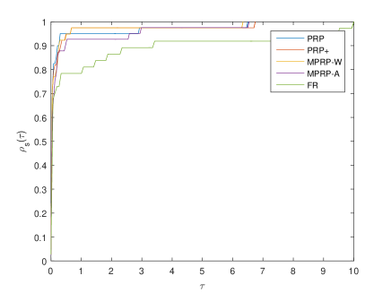
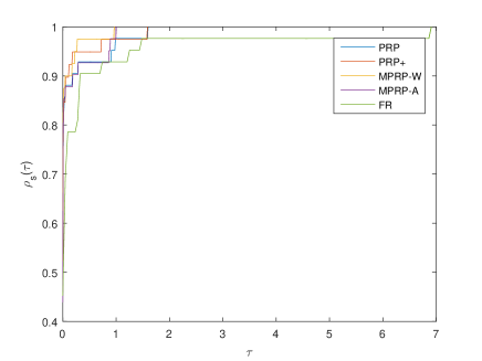

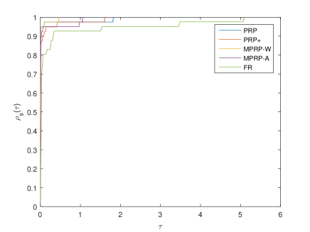
As we can see from Figure 1, overall, the four PRP methods are clearly superior to the FR methods in terms of various performance measurement. With respect to the number of iterations (Figure 1a), the MPRP-W method is the most efficient algorithm followed by the PRP method, the MPRP-A method, the PRP+ method, and the FR method. Regarding the CPU time (Figure 1b), although the PRP+ method is slightly the most efficient, it is quickly outperformed by the MPRP-W method, moreover, the MPRP-W method was the first to reach , which shows that it defeats the remaining method and is the most efficient. In term of the number of function evaluations (Figure 1c), the MPRP-W method is the most efficient and robust one followed by the PRP+ method, the MPRP-A method, the PRP method, and of these comparisons, the FR method performs the worst. Considering the number of gradient evaluations (Figure 1d), the most efficient method is also the MPRP-W method, the MPRP-A method outperforms the PRP+ method, the PRP method and the FR method to be the second most superior method in this measurement. This behaviour is justified by the fact that it generally requires a reasonable number of iterations and the implementation of its backtracking procedure does not use any additional derivative information. Figure 1 shows that the MPRP-W method performs well under all performance measurement and is an efficient way to find Pareto points.
From the experiments stated above, it can be seen that the MPRP-W method performs quite well under the four performance measurement: (A) Number of iterations; (B) CPU time; (C) Number of function evaluations; (D) Number of gradient evaluations.
6. Conclusion
In this paper, we proposed and analyzed a nonlinear modified Polak-Ribière-Polyak type conjugate gradient method with a nonnegative conjugate parameter to find critical points of vector-valued functions with respect to the partial order induced by a closed, convex, and pointed cone with nonempty interior. This variant are nontrivial extensions of a new Polak-Ribière-Polyak type method of the scalar case to the vector setting. We showed that the search direction in our method satisfies the sufficient descent condition independent of any line search. Furthermore, under mild assumptions, we obtained the results of global convergence with the standard Wolfe line search conditions as well as the standard Armijo line search strategy without convexity assumption of the objective functions. Numerical experiments showed that the effectiveness of the proposed method.
References
- [1] R. Fletcher and C. M. Reeves, Function minimization by conjugate gradients, The Computer Journal, 7(1964), 149-154.
- [2] R. Fletcher, Unconstrained optimization, Practical Methods of Optimization, 1(1980).
- [3] Y. H. Dai and Y. Yuan, A nonlinear conjugate gradient method with a strong global convergence property, SIAM Journal on Optimization, 10(1999), 177-182.
- [4] E. Polak and G. Ribière, Note sur la convergence de méthodes de directions conjuguées, Revue française d’informatique et de recherche opérationnelle, Série rouge, 3(1969), 35-43.
- [5] M. R. Hestenes and E. Stiefel, Methods of conjugate gradients for solving linear systems, Journal of Research of the National Bureau of Standards, 49(1952), 409-436.
- [6] R. T. Marler and J. S. Arora, Survey of multi-objective optimization methods for engineering, Structural and Multidisciplinary Optimization, 26(2004), 369-395.
- [7] J. Jahn, A. Kirsch and C. Wagner, Optimization of rod antennas of mobile phones, Mathematical Methods of Operations Research, 59(2004), 37-51.
- [8] C. Zopounidis, E. Galariotis, M. Doumpos, S. Sarri and K. Andriosopoulos, Multiple criteria decision aiding for finance: An updated bibliographic survey, European Journal of Operational Research, 247(2015), 339-348.
- [9] Y. Jin, Multi-objective machine learning, Springer Science and Business Media, 2006.
- [10] M. Tavana, A subjective assessment of alternative mission architectures for the human exploration of Mars at NASA using multicriteria decision making, Computers and Operations Research, 31(2004), 1147-1164.
- [11] M. Gravel, J. M. Martel, R. Nadeau, W. Price and R. Tremblay, A multicriterion view of optimal resource allocation in job-shop production, European Journal of Operational Research, 61(1992), 230-244.
- [12] M. Tavana, M. A. Sodenkamp and L. Suhl, A soft multi-criteria decision analysis model with application to the European Union enlargement, Annals of Operations Research, 181(2010), 393-421.
- [13] J. A. H. N. Johannes, Scalarization in vector optimization, Mathematical Programming, 29(1984), 203-218.
- [14] D. T. Luc, Scalarization of vector optimization problems, Journal of Optimization Theory and Applications, 55(1987), 85-102.
- [15] L. M. Graña Drummond and A. N. Iusem, A projected gradient method for vector optimization problems, Computational Optimization and Applications, 28(2004), 5-29.
- [16] E. H. Fukuda and L. M. Graña Drummond, On the convergence of the projected gradient method for vector optimization, Optimization, 60(2011), 1009-1021.
- [17] E. H. Fukuda and L. M. Graña Drummond, Inexact projected gradient method for vector optimization, Computational Optimization and Applications, 54(2013), 473-493.
- [18] L. M. Graña Drummond, F. M. P. Raupp and B. F. Svaiter, A quadratically convergent Newton method for vector optimization, Optimization, 63(2014), 661-677.
- [19] T. D. Chuong, Newton-like methods for efficient solutions in vector optimization, Computational Optimization and Applications, 54(2013), 495-516.
- [20] F. Lu and C. R. Chen, Newton-like methods for solving vector optimization problems, Applicable Analysis, 93(2014), 1567-1586.
- [21] L. G. Drummond and B. F. Svaiter, A steepest descent method for vector optimization, Journal of Computational and Applied Mathematics, 175(2005), 395-414.
- [22] T. D. Chuong and J. C. Yao, Steepest descent methods for critical points in vector optimization problems, Applicable Analysis, 91(2012), 1811-1829.
- [23] H. Bonnel, A. N. Iusem and B. F. Svaiter, Proximal methods in vector optimization, SIAM Journal on Optimization, 15(2005), 953-970.
- [24] A. N. Iusem, J. G. Melo and R. G. Serra, A Strongly Convergent Proximal Point Method for Vector Optimization, Journal of Optimization Theory and Applications, 190(2021), 183-200.
- [25] W. Chen, Y. Zhao and X. Yang, Conjugate gradient methods without line search for multiobjective optimization, arXiv preprint arXiv:2312.02461.
- [26] Q. Hu, L. Zhu and Y. Chen, Alternative extension of the Hager-Zhang conjugate gradient method for vector optimization, Computational Optimization and Applications, (2024), 1-34.
- [27] M. L. Gonçalves, and L. F. Prudente, On the extension of the Hager-Zhang conjugate gradient method for vector optimization, Computational Optimization and Applications, 76(2020), 889-916.
- [28] L. R. Lucambio Pérez and L. F. Prudente, Nonlinear conjugate gradient methods for vector optimization, SIAM Journal on Optimization, 28(2018), 2690-2720.
- [29] Q. Hu, H. Zhang and Y. Chen, Global convergence of a descent PRP type conjugate gradient method for nonconvex optimization, Applied Numerical Mathematics, 173(2022), 38-50.
- [30] D. T. Luc, Theory of Vector Optimization, Springer, 1989.
- [31] W. Chen, X. Yang and Y. Zhao, Memory gradient method for multiobjective optimization, Applied Mathematics and Computation, 443(2023), 127791.
- [32] L. R. Lucambio Pérez and L. F. Prudente, A Wolfe line search algorithm for vector optimization, ACM Transactions on Mathematical Software, 45(2019), 1-23.
- [33] E. D. Dolan and J. J. Moré, Benchmarking optimization software with performance profiles, Mathematical Programming, 91(2002), 201-213.