21cm signal from Dark Ages collapsing halos with detailed molecular cooling treatment

Context.

In order to understand the formation of the first stars, which set the transition between the Dark Ages and Cosmic Dawn epochs, it is necessary to provide a detailed description of the physics at work within the first clouds of gas which, during their gravitational collapse, will set the conditions for stars to be form through the mechanism of thermal instability. Aims. Our objective is to study in detail the molecular cooling of gas in the halos preceding the formation of the first stars. We are furthermore assessing the sensitivity of the 21cm hydrogen line to this cooling channel.

Results. We present the CHEMFAST code, that we developed to compute the cosmological 21cm neutral hydrogen line inside collapsing matter overdensity. We precisely track evolution in the abundances of ions, atoms and molecules through a network of chemical reactions. Computing the molecular thermal function due to the excitation of the rotational levels of the $\rm H_{2}$ molecule, we find it strongly affects the gas temperature inside collapsing clouds of $10^{8}$ M_⊙. The gas temperature falls at the end of the collapse, when the molecular cooling takes over the heating due to gravitation. Conclusions. We find that the 21cm brightness temperature inside the collapsing cloud presents an emission feature, different from the one predicted in expansion scenario. It moreover follows the same behavior as the gas temperature, as it is also strongly affected by the molecular cooling. This makes it a promising probe in order to map the collapsing halos and thermal processes at work inside them.

Introduction

The chemistry of the early Universe has been source of large studies to determine the abundances of elements. From the primordial species abundances produced by the first nuclear reactions during the the Standard Big Bang Nucleosynthesis (SBBN) (Workman & Particle Data Group, 2022), up extending to the interstellar medium (ISM) housing a diverse array of heavier elements forged within stars. A large part of the studies is dedicated to the calculation of reaction rates that govern chemical processes, contingent on the prevailing environmental conditions.

From the SBBN, the Universe was completely ionized since the first elements and free electrons remained thermally coupled with photons, and their interactions made impossible for any neutral atom to form. However, as the Universe expanded, the effectiveness of matter-radiation coupling diminished, allowing ion-electron reactions to dominate. Consequently, this led to the progressive recombination of ionized elemental forms into their neutral counterparts. Simultaneously, despite their much lower reaction rates due to the necessary amount of energy, molecules also began to form.

Species abundance estimation is a central problem of any coupled reaction network. One of the first detailed models of molecular synthesis were proposed by Solomon & Klemperer (1972) who computed molecular abundances in diffuse interstellar clouds, and by Herbst & Klemperer (1973) who studied the formation of molecules in dense dark clouds. The article of Prasad & Huntress (1980),which gave a comprehensive library consisting of over 1400 reactions for 137 species, presented a first model for gas phase chemistry in interstellar clouds. The UMIST Database(Le Teuff et al., 2000; McElroy et al., 2013), contains the updated rate coefficient, temperature ranges and temperature dependence of 6173 gas-phase reactions important in astrophysical environments. However at early epochs, where a total absence of dust grains appears justified, the chemistry is different from the typical interstellar medium chemistry.

From the exhaustive work of Bates (1951) on the radiative association rate, Takayanagi & Nishimura (1960), Hirasawa (1969), Takeda et al. (1969), Saslaw & Zipoy (1967) and Matsuda et al. (1969) pointed out the way of H₂ formation through H${}_{2}^{+}$ and H^- without grains in the early Universe. Numerous reviews of the primordial chemistry were developed such as Shchekinov & Entel (1983), Lepp & Shull (1984), Dalgarno & Lepp (1987), Black (1990), Latter & Black (1991), Shapiro (1992), Puy et al. (1993), Palla et al. (1995), Stancil et al. (1996), Bougleux & Galli (1997), Stancil et al. (1998), Galli & Palla (1998), Galli & Palla (2002), Lepp et al. (2002)) and Pfenniger & Puy (2003).

Probing the Universe history between the Cosmic Microwave Background (CMB) up to the light of the first stars, during the so-called Dark Ages, is very challenging because almost no signals are emitted from these times. During this epoch, baryonic matter predominantly existed in a neutral state, as the Compton coupling with radiation waned with cosmic expansion. The 21cm hydrogen line, arising from hyperfine spin-flip transitions in neutral hydrogen atoms, offers a promising avenue for probing the Dark Ages Burns et al. (2019); Mondal & Barkana (2023). Theoretical predictions indicate an absorption feature in the CMB spectrum, which only depends of the cosmology and the thermal history of the universe.

However, observing the 21cm line during the Dark Ages is exceptionally challenging due to contamination by galactic and extra-galactic foregrounds , which are orders of magnitude more intense than the signal. A lot of efforts are put into space or moon-based experiments, e.g. Goel et al. (2022);Shi et al. (2022), which are all in very preliminary stages. The global signal measure in the following eras, during Cosmic Dawn (CD) and Epoch of Reionization EoR), could also contribute to constrain the physics of the Dark Ages, allowing or excluding models going beyond $\Lambda\rm CDM$ cosmology see Sarkar et al. (2022), Flitter & Kovetz (2022), Flitter & Kovetz (2023). The detection claimed by the Experiment to Detect the Global Reionization Signature, (Monsalve et al., 2019), which indicates a significant deviation from $\Lambda\rm CDM$ model predictions and could be explained by exotic interactions in the dark sector, remains highly controversial as it was not confirmed by the Shaped Antenna measurement of the Background RAdio Spectrum (SARAS) experiment, see Nambissan et al. (2021); which tried to repeat the same observation.

The 21cm line is also very promising for observing and characterising the first structures, Iliev et al. (2002), Novosyadlyj et al. (2020), Furugori et al. (2020). Indeed, The formation of large scale structure is today an outstanding problem in cosmology. Structure formation initiates from the growth of small positive density fluctuations. The linear theory of perturbation, applied to the uniform isotropic cosmological situation, is now well understood. It is based on the assumption that the Universe differs only slightly from a background model with uniform density at early epochs. But as these fluctuations grow, their density contrast approaches unity, and their behavior differs from the linear perturbations theory. These overdense regions evolve non-linearly, and are expected to drop out of the expansion of the universe, see Peebles (1980), Padmanabhan (2002). Overdense regions collapse from their own gravity, forming the first bound structures of the universe, and setting the conditions for the appearance of the first stars, Yoshida et al. (2006), Trenti & Stiavelli (2009), Glover (2013),Bromm (2013). In particular, they require a cooling of the baryonic gas within the collapsing structure. The main cooling vector is the significant presence of molecules, which by excitation of their rotational levels influence the temperature of the gas and encourage fragmentation in primordial clouds.

We have developed the code CHEMFAST initiated by Denis Puy, Daniel Pfennigger and Patrick Vonlanthen (Puy et al., 1993; Pfenniger & Puy, 2003; Vonlanthen et al., 2009).the main objective of this code is to compute the abundances of atomic and molecular species in the context of cosmological expansion of the universe. We incorporated the computation of the global 21cm line signal arising from atom collisions during the Dark Ages.
Then, by changing the equations of dynamics in the code, we follow a collapse scenario of overdense region of $10^{6}$-$10^{9}$ solar masses modeling the region with a simple homogeneous spherical model, including the gas pressure (Lahav, 1986; Puy & Signore, 1996). We emphasize the cooling effects on the baryonic gas arising from molecules during the collapse. We additionally compute the 21cm signal from the forming primordial cloud, highlighting its distinct features compared to the global signal of the expanding universe.

This article is organized as follows. In Section 1 we start by developping the reaction network and equations of dynamics in the expanding universe, enabling the computation of atomic and molecular abundances. In section 2 we introduce the physics of the 21cm global signal. We then analyse the key characteristics of the 21cm global signal from the Dark Ages. In Section 3 we describe the collapsing cloud model, as well as the thermal molecular functions, and subsequently present the results for the 21cm signal in this context. We conclude and outline future research directions in Section 4. Throughout this paper, we adopt the $\Lambda\rm CDM$ cosmology, and adopt the parameters values from Planck2018 Collaboration (2020) TT,TE,EE+lowE+lensing best-fit.

1 Primordial baryons in $\Lambda$CDM Universe

1.1 Reactions in baryonic gas

The SBBN model for the Universe predicts the nuclei abundances of mainly hydrogen, helium and lithium and their isotopes. The chemistry of the early Universe is the chemistry of these light elements and their respective isotopic form.

The ongoing physical reactions are numerous after the nucleus recombination, partly due to the presence of the cosmic microwave background (CMB) radiation, see Stancil & Dalgarno (1998). These reactions fall into three distinct categories, collisional, electronic, and photo-processes:

• Collisional reactions $\xi+\xi^{\prime}\longleftrightarrow\xi_{1}+\xi_{2}$
  involve processes such as association, associative detachment, mutual neutralization, charge exchange, and reverse reactions.
  

• Electronic reactions $\xi+{\rm e}^{-}\,\longleftrightarrow\xi_{1}+\xi_{2}$
  encompass recombination, radiative attachment, and dissociative attachment processes.
  

• Photo-processes $\xi+\gamma\,\longleftrightarrow\xi_{1}+\xi_{2}$
  include dissociation, detachment, ionization, and radiative association reactions, with $\gamma$ being a photon.

The chemical kinetic of a reactant $\xi$, which leads to the products $\xi_{1}$ and $\xi_{2}$, imposes the following evolution of the average numerical density $\overline{n}_{\xi}$ (number of species $\xi$ per cm³ in the homogeneous Universe i.e. mean density):

$$\Bigr{(}\frac{{\rm d}\overline{n}_{\xi}}{{\rm d}t}\Bigl{)}_{\rm chem}\,=\,\sum_{\xi_{1}\xi_{2}}k_{\xi_{1}\xi_{2}}\,\overline{n}_{\xi_{1}}\overline{n}_{\xi_{2}}-\sum_{\xi^{\prime}}k_{\xi\xi^{\prime}}\overline{n}_{\xi}\overline{n}_{\xi^{\prime}}.$$ (1)

Here, $k_{\xi_{1}\xi_{2}}$ represents the reaction rate of the $\xi$-formation process from $\xi_{1}$ and $\xi_{2}$, and $k_{\xi\xi^{\prime}}$ denotes the reaction rate of $\xi$-destruction by collision with the reactant $\xi^{\prime}$.
The typical rate of collisional reactions, denoted as $k_{\rm coll}$ (in cm³ s^-1), is calculated by averaging cross sections $\sigma(E)$ over a Maxwellian velocity distribution at temperature $T_{\rm k}$:

$$k_{\rm\xi,\xi^{\prime}}=\sqrt{\frac{8}{\pi m_{\rm r}}}\,\Bigr{[}k_{\rm B}T_{\rm k}\Bigl{]}^{-3/2}\int_{0}^{\infty}\sigma(E)\,{\rm e}^{-E/k_{B}T_{\rm k}}\,E\,{\rm d}E$$ (2)

where $E$ is the collision energy, $m_{\rm r}$ the reduced mass of the collisional system ($\xi,\xi^{\prime}$), $T_{\rm k}$ the kinetic baryonic temperature and $k_{\rm B}$ the Boltzmann constant.
The radiative rate coefficient $k_{\rm rad}$ (in s^-1) which depends on the radiative cross section, $\sigma_{\rm rad}$ at the frequency $\nu$, and on the CMB, is defined by

$$k_{\rm rad}=\frac{8\pi}{c^{2}}\,\int_{\nu_{\rm th}}^{\infty}\sigma_{\rm rad}(\nu)\ \frac{\nu^{2}\,{\rm d}\nu}{{\rm exp}(h_{\rm P}\nu/k_{\rm B}T_{\rm r})-1}$$ (3)

where $\nu_{\rm th}$ is the threshold frequency above which the radiative process is possible and $T_{\rm r}$ the radiation temperature. $c$ is the speed of light and $h_{\rm P}$ the Planck’s constant. References of the different reaction rates are given in Table 1.

1.2 Dynamical evolution

To track the abundance of atomic and molecular species throughout the Universe’s evolution, it is necessary to also calculate the temporal evolution of radiation temperature, baryon temperature, and their average density. This involves solving a system of coupled differential equations, which we expose below.

Baryon number density

The mean numerical density of baryons, $\overline{n}_{\rm b}$, is expressed by

$$\overline{n}_{\rm b}\,=\,\sum_{\xi}\,\overline{n}_{\xi}\,=\,\frac{\sum_{\xi}N_{\xi}}{V}\ ,$$ (4)

where $N_{\xi}$ is the number count of species $\xi$, and $V$ is a comoving volume, proportional to the cube of the scale factor: $V\equiv a^{3}$. Thus the evolution of the mean number density is given by:

$$\frac{{\rm d}\overline{n}_{\rm b}}{{\rm d}t}\,=\,-3H\overline{n}_{\rm b}+\sum_{\xi}\Bigr{(}\frac{{\rm d}\overline{n}_{\xi}}{{\rm d}t}\Bigl{)}_{\rm chem}$$ (5)

where $H(t)=\dot{a}/{a}$ is the Hubble parameter. The second term in the right hand side of this equation accounts for the variation of the number of particles due to the chemical reactions, detailed in equation (1).

Species densities

For each chemical component $\xi$ we have

$$\frac{{\rm d}\overline{n}_{\xi}}{{\rm d}t}=-3H(t)\,\overline{n}_{\xi}+\Bigr{(}\frac{{\rm d}\overline{n}_{\xi}}{{\rm d}t}\Bigl{)}_{\rm chem}$$ (6)

where $\overline{n}_{\xi}$ is the numerical density $\xi$. The last term of the second member of this equation express the contribution of the chemical kinetics (see Eq. (1)).

Radiation temperature

In an expanding universe, the energy density of radiation evolves as $\rho_{r}\propto(1+z)^{4}$. The CMB can be likened to a black body, and Stefan-Boltzmann’s law can be used to relate its temperature to its energy density: $\rho_{r}\propto T^{4}$. This leads to the following equation $T_{r}(z)=T_{r,0}(1+z)$, where $T_{r,0}=2.725\rm K$ is the blackbody temperature of the CMB. We can then deduce the evolution law:

$$\frac{dT_{r}}{dt}=-H(t)T_{r}$$ (7)

Gas temperature

The total energy density $\varepsilon_{\rm tot}$ is given by

$$\varepsilon_{\rm tot}\,=\,\varepsilon_{\rm r}+\varepsilon_{\rm th}$$ (8)

where

$$\varepsilon_{\rm r}=a_{\rm r}T_{\rm r}^{4}(1+f_{\nu})\ :\ {\rm radiative\ energy\ density}$$

$$\varepsilon_{\rm th}=\frac{3}{2}\overline{n}_{\rm b}k_{\rm B}T_{\rm k}\ :\ {\rm thermal\ energy\ density}$$

$a_{\rm r}$ is the radiation density constant. The neutrino contribution to the radiation density for $N_{\nu}$ massless, non degenerate, neutrino types is noted by $f_{\nu}$ such as:

$$f_{\nu}=\frac{7}{8}\times\Bigr{(}\frac{4}{11}\Bigl{)}^{4/3}\times N_{\rm\nu}\ .$$

The first law of thermodynamics imposes

$$\frac{{\rm d}}{{\rm d}t}\Bigr{[}\varepsilon_{\rm tot}V\Bigl{]}=-p_{\rm tot}\,\frac{{\rm d}V}{{\rm d}t}+\frac{\delta Q}{\delta t}\ .$$ (9)

$p_{\rm tot}$ is the total pressure, which depends on $p_{\rm r}$ (radiative pressure) and $p_{\rm m}$ (pressure of baryonic gas):

$$p_{\rm tot}\,=\,p_{\rm r}+p_{\rm m}\,=\,\frac{a_{\rm r}T_{\rm r}^{4}}{3}(1+f_{\nu})+\overline{n}_{\rm b}k_{\rm B}T_{\rm k}\ .$$ (10)

$\delta Q$ is the external contribution and defined by (we neglect the role of enthalpy reaction):

$$\delta Q=\Bigr{(}\Psi_{\rm com}+\Psi_{\rm mol}\Bigl{)}V\ .$$ (11)

$\Psi_{\rm com}$ is the energy transfer from the radiation to matter via Compton scattering of CMB photons on free electrons, see Weymann (1965) and Peebles (1968), and given by:

$$\Psi_{\rm com}\,=\,4\overline{n}_{\rm e}\sigma_{\rm T}a_{\rm r}k_{\rm B}T_{\rm r}^{4}\,\frac{T_{\rm r}-T_{\rm k}}{m_{\rm e}c}\,.$$ (12)

$\sigma_{T}$ defines the Thomson cross-section, $m_{\rm e}$ the electron mass and $\overline{n}_{\rm e}$ the mean numerical electron density.
$\Psi_{\rm mol}$ defines the energy transfer via excitation and de-excitation of molecular rotational transition. This process is detailed in Section (1.4). We deduce the evolution of the baryons temperature $T_{\rm m}$ in a comoving frame:

$$\frac{{\rm d}T_{\rm k}}{{\rm d}t}\,=\,\frac{2}{3\overline{n}_{\rm b}k_{\rm B}}\Bigl{(}\Psi_{\rm adia}+\Psi_{\rm com}+\Psi_{\rm mol}\Bigr{)}$$ (13)

where $\Psi_{\rm adia}$ is the adiabatic cooling due to the expansion is given by :

$$\Psi_{\rm adia}\,=\,-3H(t)n_{\rm b}k_{\rm B}T_{\rm k},$$ (14)

where $H(t)$ is the Hubble parameter. Moreover we have a last equation which translates the conversion between time and redshift dependence :

$$\frac{dz}{dt}=-H(z)(1+z)$$ (15)

The set of equations (5,6,7,13,15) are coupled and must be solved simultaneously.

1.3 Numerical approach

The search for solution of the initial value problem, for systems of ordinary differential equations, is a typical stiff problem. Gear methods have excellent stability properties and are widely used for solving chemical kinetic problems then estimating the molecular abundances, Gear (1971), Hindmarsh & Petzold (1995). Primordial abundances can vary of 50 orders of magnitude. Thus at each integration steps we must evaluate summations or differences of very small quantities, which involve a careful analysis. Summation of floating-point numbers is ubiquitous in numerical analysis and has been extensively studied, Higham (1993). In CHEMFAST we have rearranged the summation in order to calculate the differential abundances and minimize the numerical summation errors. Following this scheme we can evaluate the very low abundances of chemical components. We adopt the initial abundances of atoms and ions out of the primordial nucleosynthesis theoretical predictions, base on recent determinations of ${}^{4}H_{e}$ abundances, see Pitrou et al. (2018) : $[D/H]\sim 2.46\times 10^{-5}$, and the helium mass fraction $Y_{p}$ = 0.24709. We do not consider the lithium components. The initial abundance of primordial Lithium nucleus is too low to play a significant role in the chemical network for the highlight (see Signore & Puy, 2009).

We start our calculations in a fully ionized Universe, at redshift $z_{\rm i}=10^{4}$. This redshift corresponds to the age of the Universe at $t_{\rm i}$, where $x=1+z$ :

$$t_{\rm i}\,=\,\frac{1}{H_{0}}\,\int_{1+z_{\rm i}}^{\infty}\,\frac{{\rm d}x}{x\,\sqrt{\Omega_{\rm r,0}x^{4}+\Omega_{\rm m,0}x^{3}+\Omega_{\Lambda,0}}}\ .$$ (16)

We stop our calculations at redshift $z_{\rm f}=10$, around the beginning of the reionization (Barkana & Loeb, 2001), as this process is out of the scope of this work.

Finally, the initial numerical density of baryons $n_{\rm b,i}$ (i.e number of baryons per cm³ at $z_{\rm i}$) is computed from the cosmological model :

$$\overline{n}_{\rm b,i}\,=\,\frac{3H_{0}^{2}\,\Omega_{\rm b,i}}{8\pi G\,\mu_{\rm b}m_{\rm p}}\,=\,\frac{3H_{0}^{2}\,\Omega_{\rm b,0}}{8\pi G\,\mu_{\rm b}m_{\rm p}}\,(1+z_{\rm i})^{3}\ ,$$ (17)

where $m_{\rm p}$ is the mass of a proton, $\mu_{\rm b}$ is the molecular weight per baryonic particle. The molecular weight depends on the BBN initial conditions, and is computed as (Seager et al., 1999) :

$$\mu_{b}=\frac{1}{(1+f_{He})(1-Y_{p})},$$ (18)

where the helium number fraction $f_{He}$ is given by

$$f_{He}=\frac{n_{He}}{n_{H}}\,=\,\frac{m_{H}}{m_{He}}\,\frac{Y_{p}}{1-Y_{p}}.$$ (19)

1.4 Species abundances and thermal history

Reaction network

The chemical network, meaning every reaction between atoms, ions and moelcules that we take into account to compute the species abundances, is described in Table 1. The fitting formula of the reaction rates are mainly taken from the compilation given by Schleicher et al. (2008) , with the exception of the hydrogen and deuterium recombination which are calculated from the rate given by Novosyadlyj et al. (2022). We summarize in Table 1 the reactions and their references.

	Reaction	Reference		Reaction	Reference
(H1)	$\rm{H^{+}+e^{-}\rightarrow H+\gamma}$	NKMS22	(H2)	$\rm{H+\gamma\rightarrow H^{+}e^{-}}$	AAZ97
(H3)	$\rm{H+e^{-}\rightarrow H^{-}+\gamma}$	GP98	(H4)	$\rm{H^{-}+\gamma\rightarrow H+e^{-}}$	GP98
(H5)	$\rm{H^{-}+H\rightarrow H_{2}+e^{-}}$	GP98	(H6)	$\rm{H^{-}+H^{+}\rightarrow H_{2}^{+}+e^{-}}$	GP98
(H7)	$\rm{H^{-}+H^{+}\rightarrow H+H}$	LSD02	(H8)	$\rm{H+H^{+}\rightarrow H_{2}^{+}+\gamma}$	GP98
(H9)	$\rm{H_{2}^{+}+\gamma\rightarrow H+H^{+}}$	GP98	(H10)	$\rm{H_{2}^{+}+H\rightarrow H_{2}+H^{+}}$	GP98
(H11)	$\rm{H_{2}^{+}+e^{-}\rightarrow H+H}$	GP98	(H12)	$\rm{H_{2}^{+}+\gamma\rightarrow H^{+}+H^{+}+e^{-}}$	GP98
(H13)	$\rm{H_{2}+H^{+}\rightarrow H_{2}^{+}+H}$	SKHS04	(H14)	$\rm{H_{2}+e^{-}\rightarrow H+H^{-}}$	CCDL07
(H15)	$\rm{H_{2}+e^{-}\rightarrow H+H+e^{-}}$	TT02	(H16)	$\rm{H_{2}+\gamma\rightarrow H_{2}^{+}+e^{-}}$	GP98
(A2)	$\rm{H^{-}+H_{2}^{+}\rightarrow H_{2}+H}$	AAZN97
(D1)	$\rm{D^{+}+e^{-}\rightarrow D+\gamma}$	NKMS22	(D2)	$\rm{D+\gamma\rightarrow D^{+}+e^{-}}$	AAZ97
(D3)	$\rm{D+H^{+}\rightarrow D^{+}+H}$	Savin (2002)	(D4)	$\rm{D^{+}+H\rightarrow D+H^{+}}$	Savin (2002)
(D5)	$\rm{H+D\rightarrow HD+\gamma}$	GP98	(D6)	$\rm{D+H_{2}\rightarrow H+HD}$	GP02
(D7)	$\rm{HD^{+}+H\rightarrow H^{+}+HD}$	SLD98	(D8)	$\rm{D^{+}+H_{2}\rightarrow H^{+}+HD}$	GP02
(D9)	$\rm{HD+H\rightarrow H_{2}+D}$	GP02	(D10)	$\rm{HD+H^{+}\rightarrow H_{2}+D^{+}}$	GP02
(D11)	$\rm{D+H^{+}\rightarrow HD^{+}+\gamma}$	GP98	(D12)	$\rm{H+D^{+}\rightarrow HD^{+}+\gamma}$	GP98
(D13)	$\rm{HD^{+}+\gamma\rightarrow H+D^{+}}$	SGP+08	(D14)	$\rm{HD^{+}+\gamma\rightarrow H^{+}+D}$	SGP+08
(D15)	$\rm{HD^{+}+e^{-}\rightarrow H+D}$	SLD98
(He1)	$\rm{He^{++}+e^{-}\rightarrow He^{+}+\gamma}$	GP98	(He2)	$\rm{He^{+}+\gamma\rightarrow He^{++}+e^{-}}$	GP98
(He3)	$\rm{He^{+}+e^{-}\rightarrow He+\gamma}$	GP98	(He4)	$\rm{He+\gamma\rightarrow He^{+}+e^{-}}$	GP98
(He5)	$\rm{He+H^{+}\rightarrow He^{+}+H}$	GP98 & GJ07	(He6)	$\rm{He^{+}+H\rightarrow He+H^{+}}$	ZDKL89

Table 1: Chemical reaction implemented in CHEMFAST and references used for their rates.
Acronyms : AAZ97 : Abel et al. (1997), CCDL07 : Capitelli et al. (2007), GP98 : Galli & Palla (1998), GP02 : Galli & Palla (2002) , LSD02 :Lepp et al. (2002) , NKMS22 : Novosyadlyj et al. (2022), SGP+08 : Schleicher et al. (2008), SKHS04 : Savin et al. (2004), SLD98 : 1998, ZDKL89: Zygelman et al. (1998).

Recombination

The cosmological recombination process was not instantaneous, because the electrons, captured into different atomic energy levels, could not cascade instantaneously down to the ground state. The universe expanded and cooled faster than recombination could be completed, and a small fraction of free electrons and protons remained. Recombination processes become dominant when the reactions of photoionization are negligible. We define the redshift of recombination $z_{\rm rec}$, the time at which the abundance of a neutral species is equal to the one of his corresponding ion. In Figure 1, we show the evolution of the relatives abundances (i.e the ratio of species numerical densities over the total baryonic numerical densities) of all the atomic species considered in our reaction network. We find the successive redshifts of recombination of He²⁺ ($z_{{\rm rec,He}^{2+}}\sim 5977$), He⁺ ($z_{{\rm rec,He^{+}}}\sim 2556$),D⁺ and H⁺ ($z_{{\rm rec,D^{+}}}=z_{{\rm rec,H^{+}}}\sim 1387$). The flatness of the atomic relatives abundances at $z<100$ is caused by the inefficiency of collisional reactions due the expansion of the Universe. It causes a decrease of species densities and freezes the relative abundances.

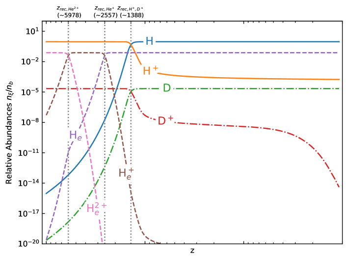
Figure 1: Relative numerical densities of atomic and ion species with respect to the total density of baryons, as a function of redshift. The computation goes from z=$10^{4}$ to $z=10$. We indicate the recombination redshifts of primordial helium, deuterium and hydrogen nuclei (He²⁺, He⁺, then D⁺ and H⁺) with vertical dotted line.

Molecular species

Molecular Hydrogen

After the freeze-out of the relative abundances due to the expansion of the universe, we obtain relatives abundances abundances and for the molecules $H_{2}$ and HD. Despite the absence of any surfaces or dust grains, it is possible to form neutral molecules through the radiative association between two neutral atoms. Molecular hydrogen cannot form directly by this radiative process, because H₂ does not have a permanent dipole moment. Charge transfer from H${}_{2}^{+}$ become the only alternative. Once H_eH⁺ was formed, this ion became an important source of H${}_{2}^{+}$ production through the exchange reaction with some neutral H. Then, H${}_{2}^{+}$ charge transfer with a neutral species led to H₂ molecules. Moreover as the radiation temperature decreases, H₂ can be formed through H^- by radiative attachment (H - e^-) followed by associative detachment (H^- - H), see Field (2000). Stimulated H^- formation (H - e^-) by CMB photons was suggested by Stancil & Dalgarno (1998), however the enhancement is relatively small, as the other alternative of H₂ formation by radiative association of excited hydrogen pointed out by Latter & Black (1991). The two major routes of H₂ formation are visible in Fig. 2 through the two jumps at the redshifts $z\sim 500$ (H${}_{2}^{+}$ channel) and $z\sim 150$ (H^- channel). After the freeze-out of the relative abundances, we find $n_{\rm rel}(\rm H_{2})=2.0$ $10^{-6}$ for the $H_{2}$ molecule. Notice that H${}_{3}^{+}$ appeared in the early Universe. H${}_{3}^{+}$ reactions, which are pivotal to the chemistry of dense interstellar clouds (see Oka (1980), Tennyson (1995) and Herbst (2000)), do not play an important role in primordial chemistry.

Molecular Deuterium

Deuterated-hydrogen molecules have permanent dipole moments which provide them the capacity to be formed by radiative association (forbidden between two hydrogen atoms). Nevertheless, HD formation is significative when H₂ appeared, as mechanism of dissociative collision (H₂ - D⁺) becomes efficient see Palla et al. (1995), Stancil & Dalgarno (1998) and Signore & Puy (2009). Due to the slight difference between the electronic structure of D and H, H₂ and HD significantly appeared at the same epoch, see Fig. 2. The relative abundance of the HD molecule lies at $n_{\rm rel}(\rm HD)=6.1$ $10^{-10}$ after the freeze-out.

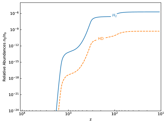
Figure 2: Relative numerical densities of molecular species with respect to the total density of baryons, as a function of redshift. The computation goes from z=$10^{4}$ to $z=10$.

Molecular thermal functions

The formation of primordial molecules such as $\rm H_{2}$ and $\rm HD$ generates thermal responses due to the excitation of rotational and vibrational levels of molecules. In the range of kinetic and radiation temperature considered, only the rotational levels can be excited. Rotational level populations depend on collisional reactions, and radiative processes (CMB absorption or induced and spontaneous emission). Two mechanisms are able to excite or de-excite molecules rotational levels. A molecule can be radiatively excited from a level $J$ to a superior one $J^{\prime}$, by absorbing a photon external to the medium (for instance from the radiative background), then desexcite via a collision with another atom or molecule from the medium. The external photon energy in converted into kinetic energy, hence we consider a molecular heating. A molecule can be also excited by collision from a level $J$ to $J^{\prime}$, then emit a photon by spontaneous or induced desexcitation to the $J$ level. If the photon isn’t reabsorbed by the medium, the associated energy is lost, and we can talk about molecular cooling.

To express the energy per volume unit that can be gained $\Gamma_{\rm mol}$ (heating) or lost $\Lambda_{\rm mol}$ (cooling) by the medium due to rotational level transitions, we define the thermal molecular function :

$$\Psi_{\rm mol}=\Gamma_{\rm mol}-\Lambda_{\rm mol}.$$ (20)

In the next two paragraphs, we look at how the heating and cooling terms are computed.

Molecular heating

The collisional de-excitation probability expresses the ratio between the collisional de-excitation rate and the total de-excitation rate, which includes collisions, as well induced and spontaneous emissions :

$$P^{c}_{J^{\prime},J}=\frac{n_{\xi}X_{J^{\prime}}k^{\xi}_{J^{\prime},J}}{n_{\xi}X_{J^{\prime}}k^{\xi}_{J^{\prime},J}+X_{J^{\prime}}A_{J^{\prime},J}+X_{J^{\prime}}B_{J^{\prime},J}\rho_{J^{\prime},J}}\ .$$ (21)

$n_{\xi}$ is the numerical density of the collision partner species $\xi$ and $X_{J^{\prime}}$ is the population fraction of molecule in the rotational level $J^{\prime}$ (see the Appendix for the detailed computation of $X_{J^{\prime}}$). $k^{\xi}_{J^{\prime},J}$ is the collision rate of this reaction. $A_{J^{\prime},J}$ and $B_{J^{\prime},J}$ are the Einstein coefficients for spontaneous and induced emission respectively. $\rho_{J^{\prime},J}$ is the radiation energy density. Each term of the sum is the de-excitation term associated to one of the three mentioned processes. Taking the product between the molecule density at $J$ level $n_{\rm mol}X_{J}$, the induced radiative excitation probability $B_{J,J^{\prime}}\rho_{J,J^{\prime}}$, the collisional de-excitation probability $P^{c}_{J^{\prime},J}$, and the energy difference between the two levels $\Delta\epsilon_{J^{\prime},J}=\epsilon_{J^{\prime}}-\epsilon{J}$, we can finally compute the energy gained by the medium per unit of volume and time through molecular thermal influence :

$$\Gamma_{\rm mol}=\sum_{J}\sum_{J^{\prime}}n_{\rm mol}\,X_{J}\,B_{J,J^{\prime}}\,\rho_{J,J^{\prime}}P^{c}_{J^{\prime},J}\,\Delta\epsilon_{J^{\prime},J}.$$ (22)

We sum over all the $J^{\prime}$ levels reachable by excitation, and over $J$ to take into account the contribution from all the rotational levels.

The energy of a rotational level $J$ can be computed as :

$$\epsilon_{J}=h\,BJ(J+1)\ {\rm where}\ B\ {\rm is\ the\ rotation\ constant}\ B=\frac{h}{8\pi^{2}cI},$$ (23)

with I the momentum of inertia.

Molecular cooling

By analogy, we firstly compute the radiative de-excitation probability :

$$P^{r}_{J^{\prime},J}=\frac{X_{J^{\prime}}A_{J^{\prime},J}+X_{J^{\prime}}B_{J^{\prime},J}\rho_{J^{\prime},J}}{n_{\xi}X_{J^{\prime}}k^{\xi}_{J^{\prime},J}+X_{J^{\prime}}A_{J^{\prime},J}+X_{J^{\prime}}B_{J^{\prime},J}\rho_{J^{\prime},J}},$$ (24)

which is the ratio between both induced and spontaneous radiative de-excitation rates, to the total one.

We simply change the radiative excitation probability from equation (22) to the collisional excitation probability with species $\xi$ : $n_{\xi}k^{\xi}_{J,J^{\prime}}$, and change the collisional de-excitation probability to the radiative one (24). We can then compute the energy lost by the medium per unit of volume and time through molecular thermal influence :

$$\Lambda_{\rm mol}=\sum_{J}\sum_{J^{\prime}}n_{\rm mol}\,n_{\xi}\,k^{\xi}_{J,J^{\prime}}\,X_{J}\,P^{r}_{J^{\prime},J}\,\Delta\epsilon_{J^{\prime},J}.$$ (25)

Thermal Evolution

The thermal evolution depends on the tight coupling between radiation and matter resulting Compton scattering of CMB photons on free electrons. The expansion of the Universe induces a dilution of the matter which causes a loss of efficiency in matter-radiation coupling. This allows the cosmological recombination, decreasing of free electrons abundance and accelerating the decoupling. We show in Figure 4 the evolution of mean temperature of radiation $T_{r}$ and of kinetic gas temperature $T_{k}$, where thermal decoupling is clearly visible. We introduce a decoupling redshift $z_{\rm dec,1\%}$ for which the kinetic temperature is equal to 99$\%$ of the radiation temperature $T_{k}(z_{dec,1\%})=0.99\,T_{r}(z_{dec,1\%})$. The value of this redshift is $z_{\rm dec,1\%}\sim 596$.It tells us that the thermal decoupling is progressive and not instantaneous at cosmological recombination. Far from the cosmological recombination, $z<100$, the radiation temperature tends to a behavior proportional to $(1+z)$ while the kinetic temperature evolves in $(1+z)^{2}$.

H₂ is homonuclear, which implies that it does not possess a permanent dipole moment, which strongly diminish it’s thermal effect. But as it is the most abundant molecule, the thermal function due to H₂ plays a role in numerous astrophysical media (see Le Bourlot et al. (1999)). In the post-recombination context, H₂ heats the medium, because of the transfer between the hot radiation (eg. CMB) and the cold matter ($T_{r}>T_{k}$). Nevertheless we can observe in Figure 4 than the influence of H₂ on the homogeneous thermal evolution (Eq.(13)) is negligible, (Puy et al., 1993; Pfenniger & Puy, 2003). H₂ essentially plays a role on the thermal balance of the first structure in the primordial gas (see Flower & Pineau des Forêts (2001)).

Infrared emissivities of HD were calculated by Dalgarno & Wright (1972). The existence of a permanent dipole moment and its excitation temperature (21K compared to 112K for $\rm H_{2}$) give this molecule interesting cooling properties. Puy & Signore (1997) showed, in a collapsing molecular protocloud, that HD is the main cooling agent around 200 K, confirmed by Flower et al. (2000), Nakamura & Umemura (2002). Despite being by far less abundant than $\rm H_{2}$,$\rm HD$ molecule can still provide a considerable thermal contribution at the lowest temperatures, around $T_{k}<200K$ because of its permanent dipole Puy et al. (1993) Galli & Palla (1998) Stancil et al. (1998). However as H₂, HD cooling doesn’t play a role in the evolution of the gas temperature in a homogeneous expanding universe, see Flower (2000), Galli & Palla (1998), Galli & Palla (2002). Thus thermal functions $\Psi_{\rm mol}$ (molecular) is negligible on the thermochemistry of the homogeneous Universe. We will see its importance in a scenario of gravitational collapse in Section 3.

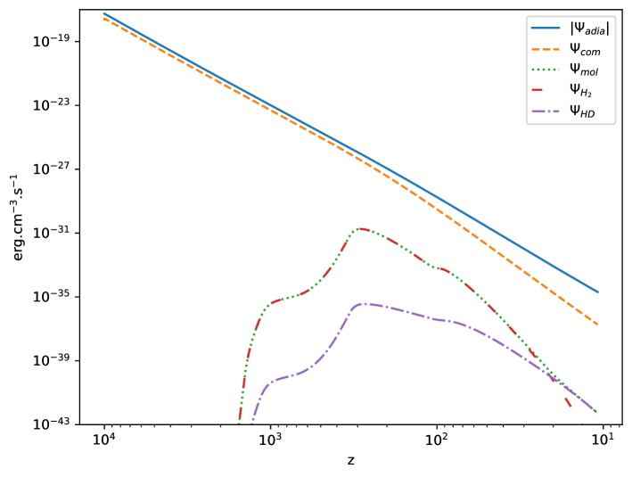
Figure 3: Evolution of cooling and heating components of the gas temperature as a function of redshift, in the homogeneous expanding universe scenario. All the components are described in terms of energy density per second. $\Psi_{\rm adia}$ arises from the expansion of the universe, as it is negative (cooling component),we display it as an absolute value. $\Psi_{\rm com}$ is due to Compton coupling between matter and radiation.$\Psi_{\rm mol}=\Psi_{\rm H_{2}}+\Psi_{\rm HD}$ corresponds to the thermal contribution of molecules H₂ and HD.

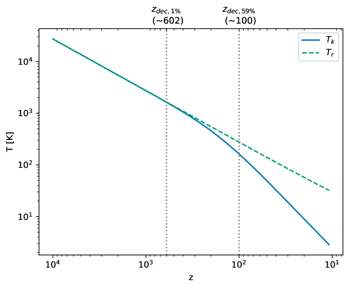
Figure 4: Evolution of radiation temperature (dotted line) and baryons temperature (full line) as a function of redshift. $z_{\rm dec,1\%}$ corresponds to the redshift at which gas and radiation temperatures are decoupled at $1\%$ : $T_{k}(z_{\rm dec,1\%})=0.99\,T_{r}(z_{\rm dec,1\%})$, in $\Lambda$CDM Universe $z_{dec,1\%}\,\sim 596$. The decoupling is a continuous process: at $z=100$, $T_{k}\sim 59\%T_{r}$, highlighted by the second vertical dotted line.

2 21cm line global signal in the Dark Ages

The hyperfine transition line of atomic hydrogen, in the ground state, arises due to the interaction between the electron and proton spins. In the excited triplet state, the spins are parallel whereas the spins in the ground (singlet) state are anti-parallel. The 21cm line is a forbidden line for which the probability for a spontaneous $1\longmapsto 0$ transition is given by the Einstein coefficient that has the value of $A_{10}=2.85\times 10^{-15}s^{-1}$ . Such an extremely small value for Einstein-A corresponds to a lifetime of the triplet state of 1.1 × 107 years for spontaneous emission. Despite its low decay rate, the 21cm transition line is expected to be one of the most important cosmological and astrophysical probes, simply due to the vast amounts of hydrogen in the Universe as well as the efficiency of collisions of H with several particles (other H, electrons and protons), and Lyman-alpha radiation from the first stars in pumping the line, establishing the population of the triplet state. Before the formation of the first astrophysical sources, only two mechanisms compete in the excitation of the hyperfine level :

$\bullet$ The Absorption and stimulated emission of photons from the CMB redshifted at the 21cm wavelength. $\bullet$ Collisions with other hydrogen atoms, free electrons and protons. In equilibrium, the relation between the number density of excited $n_{1}$ and ground state $n_{0}$ atoms is expressed by :

$$n_{1}\Bigl{(}C_{10}+P_{10}+A_{10}+B_{10}I_{\rm CMB}\Bigr{)}\,=\,n_{0}\Bigl{(}C_{01}+P_{01}+B_{01}I_{\rm CMB}\Bigr{)},$$ (26)

$C_{10}$ and $P_{10}$ are the de-excitation rates, per atom, from collisions and scattering, respectively. $C_{01}$ and $P_{01}$ correspond to the excitation rates. $I_{\rm CMB}$ is the specific intensity of CMB photons at $\nu_{10}$ and $B_{01}$ the Einstein coefficient of CMB photons absorption.
The ratio between the hyperfine population levels defines the spin temperature $T_{s}$ through :

$$\frac{n_{1}}{n_{0}}=\frac{g_{1}}{g_{0}}\exp\Bigl{(}-\frac{h{\nu_{10}}}{k_{b}T_{s}}\Bigr{)}=\frac{g_{1}}{g_{0}}\exp\Bigl{(}-\frac{T_{10}}{T_{s}}\Bigr{)}.$$ (27)

$g_{0}=1$ and $g_{1}=3$ are the statistical weights, $\nu_{10}=1420.406\,\rm MHz$ is the 21cm line rest frequency (Hellwig et al., 1970), and $T_{10}\sim 68\,\rm mK$ is the equivalent temperature of energy splitting between the two hyperfine levels.

, (28)

In the vast majority of astrophysical situations, $T_{10}<<T_{s}$, which allows write :

$$e^{-T_{10}/T_{s}}\sim 1-\frac{T_{10}}{T_{s}},$$ (29)

Hence, approximately three of four hydrogen atoms find themselves in the excited state :

$$n_{0}\sim\frac{n_{1}}{3}\sim\frac{n_{H}}{4}.$$ (30)

Since these processes are faster than the spontaneous de-excitation time of the line, we can consider than these mechanisms are in quasi-static approximation for the populations of the hyperfine levels, in the absence of radio sources. The HI spin temperature $T_{s}$ (Field, 1959) at a given redshift is a weighted mean between $T_{k}$ and $T_{r}$ and given by the equation

$$T_{s}^{-1}=\frac{T_{r}^{-1}+x_{c}T_{k}^{-1}}{1+x_{c}}\,,$$ (31)

where $x_{c}$ is the total coupling coefficient for collisions is given by the expression :

$$x_{c}=\frac{\Bigl{(}C_{H}+C_{e}+C_{p}\Bigr{)}}{A_{10}}\,\frac{T_{10}}{T_{r}}$$ (32)

where $C_{H}$, $C_{e}$ and $C_{p}$ are the de-excitation rates of the triplet due to collisions due to collisions with neutral hydrogen, electrons and protons. The collision term for each $i$ interacting species can be written as $C_{i}=n_{i}\,\kappa^{i}_{10}(T_{k})$, where $\kappa^{i}_{10}$ is the effective single-atom rate coefficient for the transition 1-0 from collisions with that species.

These rate coefficients are obtained through quantum mechanics computation for collisions with other hydrogen atoms, see Zygelman (2005), with free electrons, see Furlanetto & Furlanetto (2007a), and with protons, see Furlanetto & Furlanetto (2007b). We prefer to these tables fitting functions when possible.
Kuhlen et al. (2006) derived one for hydrogen atoms:

$$\kappa^{HH}_{1-0}(T_{k})\sim 3.1\times 10^{-11}T_{k}^{0.357}\,\exp(-32/T_{k})\rm{cm^{3}s^{-1}}$$ (33)

valid for the range 10 K$<T_{k}<10^{3}$ K. In all the computation included in this work, $T_{k}$ never reaches value beyond this range after thermal decoupling, when 21cm signal can be non-zero, so we can safely use this approximation.
For free electrons, we use a fitting function derived by Liszt (2001):

$$\log(\kappa^{eH}_{1-0}/{\rm cm}^{3}s^{-1})=-9.607+0.5\log T_{k}\times\exp[-(\log T_{k})^{4.5}/1800]\hskip 5.69054pt\,$$ (34)

which is valid for $T_{k}\leq 10^{4}$K. We keep the data tabulation from Furlanetto & Furlanetto (2007b) for the collisions with protons since there is no provided fit to our knowledge.

2.1 Brightness temperature

The equation of the radiative transfer for a specific intensity $I_{\nu}$ of photons along a path $l$, going through a cloud of hydrogen, is:

$$\frac{dI_{\nu}}{dl}=-\alpha_{\nu}I_{\nu}+j_{\nu},$$ (35)

where $\alpha_{\nu}$ and $j_{\nu}$ are the absorption and emission coefficients from the gas along the path. Defining the optical depth of the gas along the line of sight as $\tau_{\nu}=\int\alpha_{\nu}\,dl$ or $d\tau_{\nu}=\alpha_{\nu}\,dl$, we can rewrite the transfer equation :

$$\frac{dI_{\nu}}{d\tau_{\nu}}=\frac{j_{\nu}}{\alpha_{\nu}}-I_{\nu}=B_{\nu}(T)-I_{\nu},$$ (36)

As we consider the gas on the line of sight in thermal equilibrium, the emission and absorption coefficients can be expressed as a function of the temperature $T$ of the cloud only.

We can moreover relate $I_{\nu}$ at each frequency with the temperature of a blackbody of the same brightness $I_{\nu}=B_{\nu}(T_{b})$. The domain of frequency we are interested in for 21cm is low enough to lie in the application domain of the Rayleigh-Jeans approximation. Hence, we can express the intensity as a function of the equivalent brightness temperature $T_{b}$ :

$$I_{\nu}=\frac{2k_{B}T_{b}\,\nu^{2}}{c^{2}}.$$ (37)

The transfer equation becomes

$$\frac{dT_{b}}{d\tau_{\nu}}=T-T_{b}.$$ (38)

In the case of 21cm, we consider a uniform excitation temperature $T$ of the cloud, labeled spin temperature $T_{s}$. The integration of this equation leads to the following solution :

$$T_{b}(\nu)\,=\,T_{s}\Bigl{(}1-e^{-\tau_{\nu}}\Bigl{)}\,+\,T_{b}(0)e^{-\tau_{\nu}}=\,T_{s}\Bigl{(}1-e^{-\tau_{\nu}}\Bigl{)}\,+\,T_{r}e^{-\tau_{\nu}}.$$ (39)

Where the brightness temperature of the background $T_{b}(0)$ is here considered to be $T_{r}$ the CMB radiation temperature.

The actual quantity of interest for observation is the contrast between a line of sight going through high-redshift hydrogen gas and a clear line of sight to CMB. Moreover, because of cosmological redshift, the brightness temperature observed on Earth at frequency $\nu$ will be related to the actual 21cm temperature by $T_{b}(\nu)=T_{b}(\nu_{10})/(1+z)$. The contrast of brightness temperature $\delta T_{b}$ can finally be expressed as :

$$\delta T_{b}(\nu)=\frac{T_{b}-T_{r}}{1+z}=\frac{T_{s}-T_{r}}{1+z}\left(1-e^{-\tau_{\nu}}\right)\sim\frac{T_{s}-T_{r}}{1+z}\tau_{\nu},$$ (40)

where the approximation of the exponential is permitted because the optical depth for this transition is thin.

2.2 Optical depth

To compute the optical depth, we start from the integration of the absorption coefficient over the path l $\tau_{\nu}=\int\alpha_{\nu}dl$.

The absorption coefficient can be expressed with the Einstein coefficients :

$$\alpha_{\nu}=\phi(\nu)\frac{h\nu}{4\pi}\left(n_{0}B_{01}-n_{1}B_{10}\right),$$ (41)

where $\phi(\nu)$ is the normalized line profile, so that $\int\,\phi(\nu)\,d\nu=1$.
We now use the relations between the Einstein coefficients such as $g_{1}B_{10}=g_{0}B_{01}$ and $B_{10}=A_{10}\left(\frac{c^{2}}{2h\nu_{10}^{3}}\right)$, with $g_{J}$ the spin degeneracy factor for each state $J=0$ and $J=1$. We obtain :

$$\tau_{\nu}=\frac{g_{1}}{g_{0}}\frac{A_{10}}{8\pi\,\nu_{10}^{3}}c^{2}n_{0}\left(1-\frac{n_{1}\,g_{0}}{n_{0}\,g_{1}}\right)\,\int\phi(\nu)\,\nu\,dl\,.$$ (42)

Recalling from equation (30) that $n_{0}\sim n_{H}/4$, and using $\frac{n_{1}g_{0}}{n_{0}g_{1}}\sim 1-\frac{T_{10}}{T_{s}}$ we obtain

$$\tau_{\nu}=\frac{3}{32\pi}\,\frac{A_{10}}{k_{B}\nu_{10}^{2}}\,hc^{2}\,n_{H}\int\frac{\phi(\nu)}{T_{s}}\nu\,dl\,.$$ (43)

We now seek to express the integral over length to one over frequency. We first write

$$dl=c\,dt\ {\rm and}\ dt=-\frac{1}{H(z)}\,\frac{dz}{1+z},$$ (44)

where H(z) is the Hubble-Lemaître parameter. Frequency $\nu$ is affected by cosmological expansion : $\nu_{10}=\nu(1+z)$, thus we get

$$d\nu=-\nu_{10}\,\frac{dz}{(1+z)^{2}}=\nu_{10}\,\frac{H(z)}{1+z}\,dt=\frac{\nu_{10}}{c}\,\frac{H(z)}{1+z}\,dl\,=\,\frac{H(z)}{c}\,\nu\,dl.$$ (45)

Ultimately, $T_{s}$ and $H(z)$ can be pulled out of the integration because of the narrowness of the line due to its extremely slow decaying. The distance travelled by a photon from one side of the line to the other is then negligible compared to cosmological scales.
We finally obtain the following expression for the optical depth :

$$\tau_{\nu}=\frac{3hc^{3}}{32\pi}\,\frac{A_{10}}{k_{B}\nu_{10}^{2}}\,\frac{n_{H}}{H(z)\,T_{s}}.$$ (46)

2.3 Discussion

Plugging the optical depth in equation (40), we find an expression for our observable, the differential brightness temperature :

$$\delta T_{b}\sim\frac{3hc^{3}}{32\pi}\,\frac{A_{10}}{k_{B}\nu_{10}^{2}}\,\frac{n_{H}}{H\,T_{s}}\,\frac{T_{s}-T_{r}}{1+z}.$$ (47)

We have plotted, in Fig 5, the evolution of spin, radiation and kinetic temperature. The spin temperature behavior can be separated in three distincts epochs, that determine the observability of the brightness temperature, which is shown in Figure 6 :

• Before matter-radiation decoupling, the spin temperature is coupled to the CMB temperature $T_{s}=T_{r}$. Differential brightness temperature $\delta T_{b}$ remains at zero.

• Around $z\sim z_{dec,1\%}$   matter and radiation are progressively decoupling. Baryons are dense enough for the the collision mechanism to dominate in the 21cm photons production. The spin temperature is thermalized to the baryons temperature $T_{s}\rightarrow T_{k}$, and the brightness temperature reaches a minimum of $\delta T_{b}\sim-44$ mK at $z=89$. This value is in accordance with the state of the art literature, see Pritchard & Loeb (2012), Mondal & Barkana (2023).

• Due the expansion of the universe, the baryons get more and more diluted, and the collision mechanism progressively becomes ineffective. The spin temperature relaxes to the CMB temperature, $T_{s}\rightarrow T_{r}$ which brings the brightness temperatures back to zero.

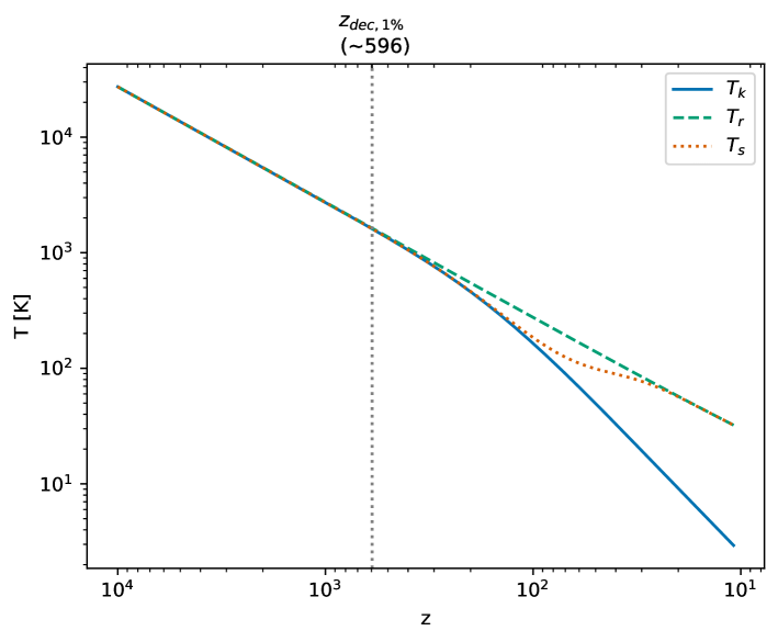
Figure 5: Evolution of kinetic temperature $T_{K}$, radiation temperature $T_{r}$ and 21cm spin temperature $T_{s}$ as a function of redshift.

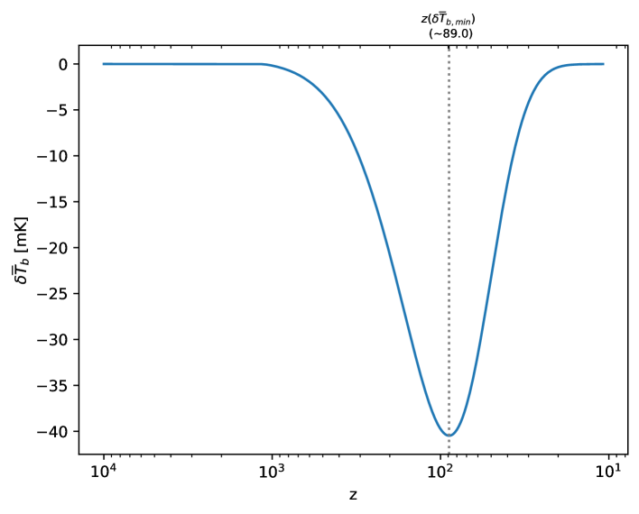
Figure 6: Evolution of the global 21cm differential brightness temperature as a function of redshift in a homogeneous expansion scenario.

With CHEMFAST, following differential equations for quantities in a homogeneous universe, we find back two important results. Firstly, the complex chemistry that takes place during and after the successive recombinations allows the first molecules to be formed, in particular $\rm H_{2}$ and HD. Their presence is crucial in explaining the cooling of the gas during the formation of the first structures. This is the subject of the next section.

Moreover, by following the thermal history of the universe and the chemical reactions, it is possible to estimate the intensity of the global 21cm signal due to the collision process during the Dark Ages. Estimating this signal is of great interest for cosmology. Its characteristics (shape, intensity, temporality) are totally independent of the astrophysical processes at work later, from Cosmic Dawn onwards. Its only dependence is therefore on cosmology Burns et al. (2019) Mondal & Barkana (2023), and to the IGM thermal history which is very sensitive to processes leading to an additional heating or cooling (e.g dark matter-baryon scattering, see Muñoz et al. (2015), or millicharged dark matter, see Muñoz & Loeb (2018)).

3 Dynamics of collapsing protoclouds and 21cm hydrogen line emission

In the context of the homogeneous expansion seen in the first part, the influence of molecules on the gas temperature is minimal, due to their very low abundance compared with other species. Their contribution is completely drowned out by the adiabatic cooling of the gas and the Compton heating associated with matter-radiation coupling. However, we know that the universe is not actually homogeneous, but has small fluctuations in density, which explains the structures present today.

In this section, we focus on the evolution of an overdensity. When a density perturbation grows enough due to gravity in order to reach a density contrast comparable to unity, it can not be described anymore par the linear theory of perturbations. To follow the evolution of these non-linear perturbations, we consider a spherical collapse model with basic hypothesis. The model we use is based on the work of Lahav (1986), extended by Puy & Signore (1996).

3.1 Model of collapsing cloud

We assume that the overdense region we follow is isothermal, spherical, and without rotation. This matter sphere, at first following the expansion of the universe, will progressively slow in its expansion compared to the background, due to the excess mass until the point when it starts to collapse back on itself. In the range of redshift we consider, the universe is fully dominated by matter, and we can assume a linear $t^{2/3}$ growth of the fluctuations with the expansion of the Universe. Hence, the spectrum of mass is given by, (see Gott & Rees, 1975) :

$$\frac{\delta\rho}{\bar{\rho}}=\left(\frac{M}{M_{0}}\right)^{-1/3}(1+z)^{-1},$$ (48)

where $M_{0}$ is defined as a characteristic mass-scale with $M_{0}=10^{15}M_{\sun}$ which is the typical mass of a super-cluster today. The density contrast at the present epoch is given by

$$\left(\frac{\delta\rho}{\rho}\right)_{0}\,=\,\left(\frac{M}{M_{0}}\right)^{-1/3}.$$ (49)

Considering a single cloud of mass $M$, we follow the collapse starting from the turnaround point, when the gravity takes over the expansion, and the perturbation starts to increase in density, as it was only diluting slower than the background before this moment. An overdense region reaches the turnaround when its density is related to the background’s one by $\rho=\Bigl{(}\frac{3\pi}{4}\Bigr{)}^{2}\bar{\rho}$ (see Padmanabhan, 2002; Peebles, 1980).
Hence the baryon number density at turnaround is expressed by

$$n_{b,ta}=\Bigl{(}\frac{3\pi}{4}\Bigr{)}^{2}\,\bar{n_{b}}(z_{ta})\,.$$ (50)

Where $\bar{n_{b}}(z_{ta})$ is the mean baryon numerical density that would have been reached at $z_{ta}$ in the homogeneous expansion case.
Following the approach of Gunn & Gott (1972) and Lahav (1986), we compute the redshift of turn-around for a given mass:

$$1+z_{ta}=\left(\frac{3\pi}{4}\right)^{-2/3}\,\left(\frac{M}{M_{0}}\right)^{-1/3}$$ (51)

This is the redshift at which we start to follow the collapse in our code. It is only dependant of the mass $M$ of the cloud.
We can also approximate that the adiabatic temperature of a monoatomic gas evolves as

$$T_{k}(z)\propto\rho_{b}(z)^{2/3}$$ (52)

in the matter-domination era. The temperature of the overdensity at turnaround can then be written as

$$T_{k,ta}=\left(\frac{3\pi}{4}\right)^{4/3}\bar{T_{k}}(z_{ta})\,.$$ (53)

Finally, the radius of the overdense region can be calculated simply from the density

$$r_{ta}=\left(\frac{3M}{4\pi\rho_{b,ta}}\right)^{1/3}\,,$$ (54)

with $\rho_{b,ta}=\mu_{b}m_{p}\,n_{b,ta}$. The collapse velocity $v_{ta}$ at the turnaround is always set at zero :

$$v_{ta}\,=\,\frac{dr_{ta}}{dt}=0.$$ (55)

For a given cloud mass value, we can directly compute the turnaround redshift $z_{ta}$, and extract the mean values $\bar{\rho_{b}}(z_{ta})$ and $\bar{T_{k}}(z_{ta})$ by running the code with the expansion parametrization from the previous sections. We then use once again the CHEMFAST code with the appropriate initial conditions. We change the set of dynamical equations in order to describe a collapse scenario of an overdense region of mass $M$, starting from the associated turnaround redshift. As in Section I, we need to solve differential evolution equations for the baryonic density, radiation temperature, gas temperature, and every reaction from the reaction network. We additionally follow the evolution of the cloud’s radius.

Baryon numerical density

The conservation of matter inside the clouds gives :

$$\frac{dn_{b}}{dt}=-3\frac{n_{b}}{r}v_{r}+\sum_{\xi}\left(\frac{dn_{\xi}}{dt}\right)_{\rm chem}\ {\rm{with}}\ v_{r}=\frac{dr}{dt}$$ (56)

The equation is similar to the expansion case of Section I, the scale factor $a$ is simply replaced by the radius of the cloud $r$. The last term of the right side of the equation is the contribution from chemical reactions.

Species densities

Similarly , for each chemical component $\xi$ we have

$$\frac{dn_{\xi}}{dt}=-3\,\frac{n_{\xi}}{r}v_{r}+\Bigr{(}\frac{{\rm d}n_{\xi}}{{\rm d}t}\Bigl{)}_{\rm chem}$$ (57)

Radiation temperature

The radiation temperature evolves just like in the homogeneous case, with the expansion of the universe:

$$\frac{dT_{r}}{dt}=-H(t)\,T_{r}$$ (58)

Gas temperature

To compute the evolution of the temperature inside the collapsing cloud, we start from the first law of thermodynamics :

$$dU=-PdV+dQ$$ (59)

Where $N_{b}$ is the total number of baryons in the cloud and $V\equiv r^{3}$ its volume, linked by $N_{b}=n_{b}V$, and $U$ the internal energy expressed by :

$$U\,=\,\frac{3}{2}\,N_{b}k_{B}T_{k}.$$ (60)

We define the pressure in the cloud assuming we are working with a perfect gas $PV=N_{b}k_{B}T_{k}$. $Q$ is the heat input of the system, defined by

$$\frac{1}{V}\,\frac{dQ}{dt}=\Psi_{\rm mol}+\Psi_{\rm com}.$$ (61)

The first right hand term $\Psi_{mol}$ expresses the thermal influence of molecules on the gas temperature through the excitation of their rotational levels (see eq. 20). The second term $\Psi_{\rm com}$ expresses the Compton coupling between matter and radiation (see eq. 12). We can finally compute the evolution of the kinetic gas temperature with respect to time:

$$\frac{dT_{k}}{dt}\,=\,\frac{2}{3n_{b}k_{B}}\left(\Psi_{\rm grav}+\Psi_{\rm mol}+\Psi_{\rm com}\right)\ {\rm{with}}\ \Psi_{\rm grav}=-3n_{b}k_{B}T_{k}\,\frac{v_{r}}{r}.$$ (62)

Radius and velocity of collapse

We start from the energy balance :

$$E=-\frac{3}{5}\frac{GM^{2}}{r}+\frac{3}{10}Mv_{r}^{2}+\frac{3}{2}N_{b}k_{b}T_{k},\ {\rm{and\,we\,know\,that}}\ \frac{dE}{dt}=\frac{dQ}{dt}.$$ (63)

Using the fact that M = $N_{b}\,\mu_{b}m_{H}$, we obtain

$$a_{r}=-\frac{GM}{r^{2}}+\frac{5k_{b}T_{k}}{\mu m_{H}}\,\frac{1}{r}\ \ {\rm{with}}\ \ a_{r}=\frac{dv_{r}}{dt}.$$ (64)

3.2 Thermal evolution of $10^{8}\rm M_{\sun}$ collapsing cloud

We focus on the analysis of a collapse of mass $10^{8}M_{\sun}$, which corresponds to the order of magnitude of mass expected for ”massive minihalos ”, the least massive halos that can still undergo molecular cooling and host star formation (see Tegmark et al., 1997; Yoshida et al., 2003; Glover, 2005; Haiman & Bryan, 2006; Trenti & Stiavelli, 2009; Greif, 2015).
For all the following figures, we display the quantities evolution as a function of the time, starting from the turn-around :

$$t_{ta}=\sqrt{\frac{3\pi}{32G\rho_{ta}}},$$ (65)

until the collapse time $t_{coll}=2t_{ta}$ (Lahav, 1986).

In Figure 7, we follow the intensity of all the energy components influencing the gas temperature within the cloud throughout its evolution in equation (62). We display the negative contributions in absolute value. The line curve, in Figure 7, corresponds to heating due to gravitational contraction $\Psi_{\rm grav}$. It gets stronger as the radius of the halo decreases and the collapse velocity increases. The dashed curve $\Psi_{\rm com}$ comes from the Compton coupling between matter and radiation. Since our initial conditions provide a gas temperature in the halo above the background radiation temperature, the Compton interaction tends to cool the gas temperature towards the radiation temperature, which explains why it has a negative contribution. The efficiency of the Compton coupling dominates over the other contributions in the first instants and decreases as the collapse progresses. It eventually becomes negligible. The $\Psi_{\rm mol}$ term (dotted curve), described above, represents the molecular thermal function. It is the sum of the $\Psi_{\rm H_{2}}$ and $\Psi_{\rm HD}$ thermal functions. The contribution to $\Psi_{\rm mol}$ is almost completely driven by $\rm H_{2}$ molecule. HD contribution becomes important for lower temperatures than the one we are interested in (¡ 200 K), hence, it doesn’t play a strong role in the case we are studying. In Figure 7, $\Psi_{mol}$ contributes to cool the gas. Initially negligible, its importance increases sharply as the density of the molecules increases and the gas temperature grows, until it becomes significant and even dominates the other thermal channels at the end of the collapse. Compared to the expansion scenario, the molecular thermal function has a strong influence on the gas temperature.

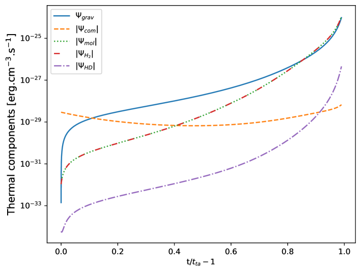
Figure 7: Evolution of cooling and heating components of the gas temperature in a $10^{8}M_{\sun}$ collapsing cloud. All components are described in terms of energy density per second. $\Psi_{\rm grav}$ arises from to gravitational collapse of the gas. $\Psi_{\rm com}$ is due to Compton coupling between matter and radiation. $\Psi_{\rm mol}=\Psi_{\rm H_{2}}+\Psi_{\rm HD}$ corresponds to the thermal contribution of molecules H₂ and HD. Negative components $\Psi_{\rm com}$, $\Psi_{\rm mol}$, $\Psi_{\rm H_{2}}$ and $\Psi_{\rm HD}$ are displayed as absolute values.

We show the evolution of the radiation and gas temperatures during the collapse in Figure 8. In the first part of the collapse, the gas temperature $T_{k}$ (lined curve) decreases. Compton coupling, which is still important, is the dominant thermal mechanism, bringing it back towards the radiation temperature (dotted curve). This mechanism is countered by heating due to the gravitational collapse of the cloud. This term provides an acceleration of the heating that takes over the Compton coupling, which itself diminishes, as the expansion of the universe progresses. In the last phase of the collapse, $T_{k}$ reaches a maximum of $1007\,\rm K$. From this point, the molecular thermal function cools the medium more than it heats up by contraction. The gas temperature decreases despite the ongoing collapse.

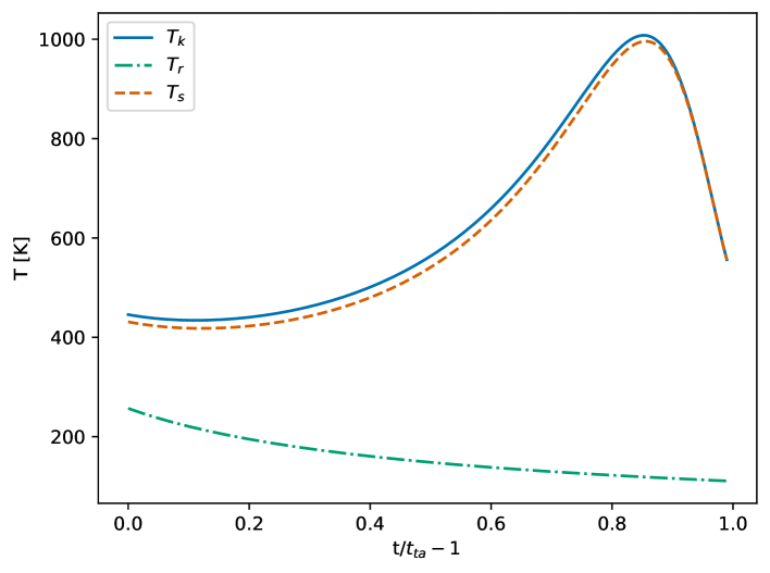
Figure 8: Evolution of radiation temperature $T_{r}$ (dash-dotted line), gas temperature $T_{k}$ (full line) and 21cm spin temperature $T_{s}$ (dotted line) for a collapsing $10^{8}$ M_⊙ cloud. The gas temperature experiences a cooling of molecular origin toward the end of the collapse.

3.3 21cm line emission from collapsing halo

In this new context of collapse, the evolution of the 21cm line signal differs from the homogeneous case. In Figure 8, spin temperature $T_{s}$ (dashed line) closely follows gas temperature $T_{k}$ throughout the collapse. Looking again at the spin temperature, see equation (31), we can explain it by the following arguments. We are in a collapse scenario, where the baryons numerical density is increased by a factor of $\sim 177$ at the end of the collapse, compared to the background. Therefore the collisional coupling is important and dominates the 21cm line production. In Figure 9, we display the brightness temperature $\delta T_{b}$ , computed by the equation (47). $\delta T_{b}$ is positive this time, which means that the signal is in emission, unlike the signal in the expansion scenario in Figure 9. Throughout the collapse, $T_{s}$ is always greater than radiation temperature $T_{r}$. The term $\left(1-\frac{T_{r}}{T_{s}}\right)$ in equation (47) therefore stays between 0 and 1. Moreover, we observe in $\delta T_{b}$ the same type of peak than for $T_{k}$, caused by molecular cooling. Indeed, since the spin temperature completely follows $T_{k}$, it is sensitive to the same thermal processes, which is transmitted to $\delta T_{b}$.

We can note that even without the activation of molecular cooling, $\delta T_{b}$ would eventually saturate and reach a maximum limit when $T_{s}\sim T_{k}\gg T_{r}$. In this regime, the dependence on $T_{s}$ in equation (47) would become unimportant. The same type of saturation is also predicted before the end of reionization, when the gas is heated by the X-rays emitted by the first sources (see e.g. Pritchard & Loeb, 2012).

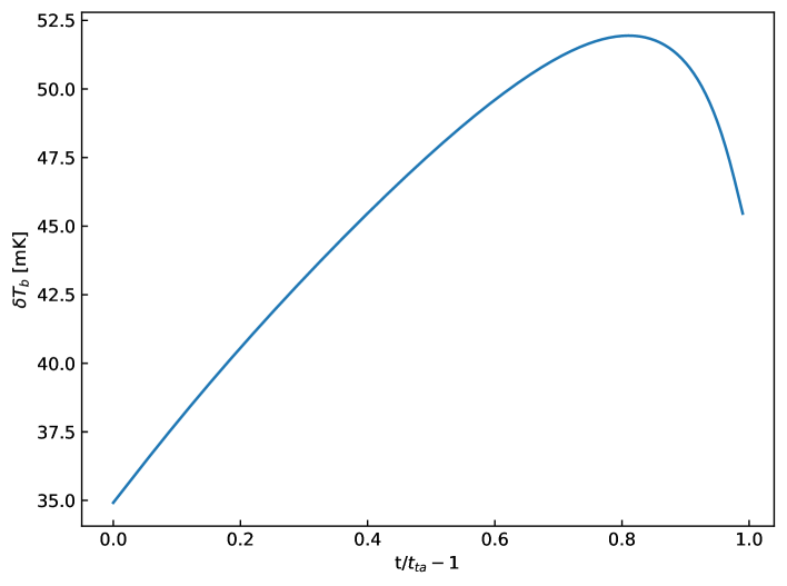
Figure 9: Evolution of the 21cm brightness temperature for a collapsing $10^{8}$ M_⊙ cloud. Unlike the homogeneous expansion scenario, the brightness temperature is positive. It additionally follows the same behavior as the gas temperature, experiencing a cooling of molecular origin toward the end of the collapse.

4 Discussion & Perspectives

We have explored in detail the evolution of species abundances during and after successive recombinations. To do so, we improved the code CHEMFAST, which solves a system of stiff coupled differential equations. One part of the system describes the dynamics (density, baryon and radiation temperatures), and another is dedicated to describing the network of collisional, electronic, and photoprocesses. Particular attention has been paid to monitoring the abundance of molecules. We have developed a calculation of the signal from the excitation of the hydrogen 21cm line, taking into account only the collisional excitation that dominates during the Dark Ages.

We first applied our code in the simple framework of an expanding homogeneous universe. Following the cosmological parameters $\Lambda\rm CDM$ from PLANCK Collaboration (2020), we compute the successive recombinations of $\rm He^{2+}$,$\rm He^{+}$ and $\rm H^{+}/\rm D^{+}$, as well as the relative abundances of all the atoms, ions and molecules contributing to the reaction network. On top of this, we implemented the 21cm line brightness temperature computation during the dark ages, taking into account the collisional excitation. It shows an absorption peak with an intensity of -40 mK at z=89. This result is largely corroborated by the literature (Furlanetto et al., 2006; Pritchard & Loeb, 2012; Mesinger, 2020) and enabled us to validate the effectiveness of our code.

In a second part, our objective was to study the development of molecular cooling, its importance in the thermal history of a collapsing primordial cloud. To this end, we flexibly integrated a new set of dynamical equations into our abundance calculation code CHEMFAST. We based ourselves on the spherical collapse model developed by Lahav (1986), with the cloud mass as the only free parameter. We have carried out collapses for masses of $10^{8}M_{\sun}$. Within the collapse, molecules are present in much greater density than in the homogeneous case. Calculating the excitation of the rotational levels for the $H_{2}$ and $HD$ molecules shows us that they have a strong thermal impact on the temperature of the gas in the cloud. We can even find a regime in the final moments of the collapse, such as this contribution becomes dominant and takes over the gravitational heating, leading to a fall of the gas temperature. This well known phenomena named ”molecular cooling” is crucial in order to explain the formation of the first stars from this kind of structures.

Indeed, molecular cooling is responsible for the development of thermal instabilities. Thermal instabilities were first studied by Parker (1953), followed by Field (1965) who derived an instability criterion, leading to a growth of the perturbations in the gas. Sabano & Yoshii (1977) found that instabilities of this type could be triggered by molecular hydrogen provoking cooling in collapsing halos. Uehara et al. (1996)studied the fragmentation of primordial clouds after the thermal decoupling and showed the important role of molecular cooling in the dynamics of collapse.

Molecular cooling mechanism is necessary in order to trigger the formation of stars within a primordial cloud. Gravitational instabilities are not sufficient to induce the fragmentation that is at the origin of star formation. On the other hand, molecular cooling can induce the appearance of instabilities of a thermal nature, highlighted for the first time in Field (1965). The aim of our simple model was to highlight the crucial thermal influence of molecules, but it does not allow us to explore the evolution of thermal instabilities in depth. We would then have to turn to Adaptive Mesh Refining (AMR) type simulations, such as the ENZO code Bryan et al. (2014). This type of approach makes it possible to spatially monitor instabilities that can lead to fragmentation within the structure. Recently Tang & Chen (2024) quantitatively examined the turbulence effect on the primordial cloud formation, and employ the ENZO code to model the gas cloud with primordial composition, including artificial-driven turbulence on the cloud scale and relevant gas physics. Their results show that turbulence with high Mach number and compressional mode effectively fragments the cloud into several clumps, each with dense cores of $22.7-174.9\,M_{\odot}$ that undergo Jeans instability to form stars.
Finally, we computed the 21cm line brightness temperature within collapsing halos. The signal shows a very different signature from the homogeneous expansion scenario. It presents an emission feature, and is also affected by molecular cooling, in the same way as the gas temperature to which the brightness temperature is coupled. These particular signatures are promising in order to probe the thermal history inside halos. They could also present an observational interest at the smallest scales of the 21cm power spectrum in the context of the forthcoming HERA and SKA observations. One way to estimate this impact would be to associate our results with a halo mass function (Lukić et al., 2007; Murray et al., 2013). But the determination of the HMF for redshifts $z>30$ is not well calibrated and makes the task challenging. Indeed, our model predicts cloud formation at particularly high redshifts compared to what is currently proposed in the literature. (e.g. Trenti & Stiavelli, 2009; Glover, 2013; Greif, 2015) propose formations redshifts around $z\sim 30$ for the lowest mass halos allowing gas collapse within them ($\sim 10^{5}-10^{6}M_{\sun}$).

Furthermore, our work is part of an effort to estimate the 21cm signal from halos. Iliev et al. (2002) were among the first to propose a model of 21cm emission in minihalos starting before reionization from collisional excitation. They found brightness temperatures of the order of $0.1K$ for an individual minihalo between $10^{4}$ and $10^{8}M\sun$ at redshifts between $7$ and $20$. More recently, Furugori et al. (2020) calculated the 21cm signal emitted by Ultracompact minihalos formed at high redshift. They find fluctuations of the order of mK at redshifts between $z=10$ and $30$. Finally Novosyadlyj et al. (2020) calculates the 21cm emission in haloes between $10^{6}$ and $10^{10}M_{\sun}$, virialized between $z\sim 10-50$. They find brightness temperatures of the order of $1-10K$ within a halo.
More recently Novosyadlyj et al. (2024) analyze the formation of the 21cm line in the Dark Ages in different non-standard cosmological models. The dependences of the amplitude of 21cm line signal to the parameters of the cosmological and first-light models are strongly degenerate. Detection by tomography of the Dark Ages, Cosmic Dawn, and Reionization epochs, in the 21cm line, would significantly reduce it. This task is a crucial challenge even for modern advanced telescopes, receivers, and technologies with nanosatellites for extracting a 21cm signal.

Appendix :Molecular rotational levels

Einstein coefficients

This appendix is mainly inspired from Puy & Signore (1997) and Vonlanthen (2009).
Let’s assume a container inside which there is a radiation field of density $\mathrm{\rho(\nu)d\nu}$ and molecules capable of passing from a rotational level $J$ to a higher level $J^{\prime}$ by the absorption of a photon whose energy $h_{\mathrm{P}}\nu_{JJ^{\prime}}$ corresponds to the energy difference between the two levels (radiative excitation) or by collision (collisional excitation). De-excitation can also be collisional or radiative (spontaneous or induced).

There are three radiative processes: spontaneous emission, induced emission and absorption. The Einstein coefficients $A_{J^{\prime}J}$ and $B_{JJ^{\prime}}$ are defined as follows:

• Spontaneous emission: the probability of spontaneous emission $A_{J^{\prime}J}$ is the probability that a molecule in the rotational state $J^{\prime}$ spontaneously emits a photon of energy $h_{\rm{P}}\nu_{JJ^{\prime}}$ corresponding to the transition from $J^{\prime}$ to $J$.

• Induced emission: The probability of induced emission is defined by the probability that the atom passes from $J^{\prime}$ to $J$ when it is subjected to induced radiation with a frequency between $\nu_{J^{\prime}}$ and $\nu_{J^{\prime}}+\mathrm{d}\nu$. This probability is denoted $B_{J^{\prime}J}\rho(\nu)$.

• Absorption: absorption occurs when a molecule in the $J$ state, exposed to isotropic radiation of density $\mathrm{\rho(\nu)d\nu}$ and frequency between $\nu_{J^{\prime}}$ and $\nu_{J^{\prime}}+\mathrm{d}\nu$, absorbs a photon of energy $h_{\rm{P}}\nu_{JJ^{\prime}}$ and changes to the $J^{\prime}$ state. We write the probability of absorption $B_{JJ^{\prime}}\rho(\nu)$.

If we write $I$ the moment of inertia of a molecule, then the energy of the rotational level $J$ is given by (Cohen-Tannoudji et al., 1973; Kutner, 1984) :

$$\epsilon_{J}=\frac{J(J+1)h_{\mathrm{P}}^{2}}{8\pi^{2}I},$$ (66)

with $h_{\rm{P}}$ the Planck constant. We can rewrite :

$$\epsilon_{J}=h_{\mathrm{P}}BJ(J+1),$$ (67)

where $B=h_{\mathrm{P}}/8\pi^{2}I$ is called the molecule’s rotation constant. We can see that the more massive a molecule is, the greater its moment of inertia will be, and therefore the smaller its rotation constant will be. Transition frequencies are obtained by taking the energy differences between two levels and dividing by $h_{\mathrm{P}}$. For dipole molecules, transitions obey the rule $\left|\Delta J\right|=1$, so that $J^{\prime}=J+1$. In this case we have:

$$\nu_{J+1,J}=\nu_{J+1}-\nu_{J}=\frac{\epsilon_{J+1}-\epsilon_{J}}{h_{\mathrm{P}}}=2B(J+1).$$ (68)

For homopolar molecules like H₂, the transition rule is $\left|\Delta J\right|=2$. Hence we get :

$$\nu_{J+2,J}=\nu_{J+2}-\nu_{J}=\frac{\epsilon_{J+2}-\epsilon_{J}}{h_{\mathrm{P}}}=2B(2J+3).$$ (69)

The Einstein coefficient $A_{J+1,J}$ can be related to the dipole moment $\mu_{\mathrm{r}}$ (Kutner, 1984):

$$A_{J+1,J}=\frac{64\pi^{4}\nu_{J+1,J}^{3}}{3h_{\mathrm{P}}c^{3}}\mu_{\mathrm{r}}^{2}\frac{J+1}{2J+3}.$$ (70)

Furthermore, the coefficients $B_{J+1,J}$ and $A_{J+1,J}$ are related by the following formula :

$$B_{J+1,J}=A_{J+1,J}\frac{c^{3}}{8\pi h_{\mathrm{P}}\nu_{J+1,J}^{3}}.$$ (71)

Finally, the probabilities of absorption and stimulated emission are also related:

$$g_{J}B_{J,J+1}=g_{J+1}B_{J+1,J},$$ (72)

where the $g_{i}$ are the statistical weights of the rotational levels $i$: $g_{i}=2i+1$.

In the case of collisional transitions, the de-excitation probability $C_{J^{\prime},J}$ is computed by the product:

$$C_{J^{\prime},J}=\tau_{\mathrm{coll}}n_{\mathrm{coll}},$$ (73)

where $\tau_{\mathrm{coll}}$ is the collision rate between the molecule and the collisional specie whose density is denoted by $n_{\mathrm{coll}}$. Assuming a Maxwellian velocity distribution, the collisional excitation probability $C_{J,J^{\prime}}$ is related to $C_{J^{\prime},J}$ by:

$$C_{J,J^{\prime}}=C_{J^{\prime},J}\frac{g_{J^{\prime}}}{g_{J}}\exp\left(h_{\mathrm{P}}\nu_{J+1,J}/k_{\mathrm{B}}T_{\mathrm{m}}\right).$$ (74)

From the above considerations we conclude that two quantities mainly determine the efficiency of the $\Psi$ thermal function of a molecular species: the dipole moment $\mu_{\mathrm{r}}$ and the rotation constant $B$. Since the Einstein coefficients depend on the square of the dipole moment, molecules for which $\mu_{\mathrm{r}}$ is large will be very efficient thermal agents. However, of the two most abundant molecules in the cosmic gas, H₂ does not have a permanent dipole moment, and the one of HD is very weak. For H₂ , rotational constant is B${}_{{\rm H}_{2}}=85.35$ K with no dipole moment $\mu_{r}({\rm H_{2}})=0$ D, while for HD we have B${}_{\rm HD}=64.30$ K and the dipole moment $\mu_{r}({\rm HD})=8.3\times 10^{-4}$ D.

Populations of the rotational levels

To calculate the thermal function of a molecule, we need to know the populations of its rotational levels $X_{J}$. When molecules have permanent electric dipole moments (along the axis of the molecule), the strongest transitions are those that obey the selection rule $|\Delta J|=1$. In the case of homopolar molecules such as molecular hydrogen, the dipole moment is zero for symmetry reasons. Transitions between rotational levels are therefore quadrupolar. This type of transition imposes the rule $|\Delta J|=2$. In this case, transitions between even-numbered levels $J$ = 0, 2, 4, … are called para transitions. Those occurring between odd levels $J$ = 1, 3, 5, … are called ortho transitions. We consider 20 rotational levels in our calculations.

H₂ Molecule

$\mathrm{H_{2}}$ is the only primordial homopolar molecule. It’s rotational constant is equal to $B_{\mathrm{H_{2}}}=170.66$ K. The radiative transition probability is given by :

$$A_{J,J-2}=7.52\cdot 10^{-13}\frac{J(J-1)(2J-1)^{4}}{2J+1}\quad\mathrm{s}^{-1}.$$ (75)

Let’s consider three consecutive rotational levels $J-2$, $J$ and $J+2$. The variation of the $J$ level population is :

$$\begin{array}[]{ccl}\frac{\mathrm{d}X_{J}}{\mathrm{d}t}&=&\underbrace{C_{J-2,J}X_{J-2}+B_{J-2,J}\rho_{J-2,J}X_{J-2}+C_{J+2,J}X_{J+2}+B_{J+2,J}\rho_{J+2,J}X_{J+2}+A_{J+2,J}X_{J+2}}_{\mathrm{Gain}}\\ &-&\underbrace{\left(C_{J,J+2}X_{J}+B_{J,J+2}\rho_{J,J+2}X_{J}+C_{J,J-2}X_{J}+B_{J,J-2}\rho_{J,J-2}X_{J}+A_{J,J-2}X_{J}\right)}_{\mathrm{Loss}},\end{array}$$ (76)

The first two terms of the second member in the RHS represent the transition from level $J$ to level $J+2$. The last three terms express the transition from $J$ to $J-2$. The $J$ level can therefore be depopulated either by transition to the $J+2$ level or by de-excitation to the lower $J-2$ level. The transitions are almost instantaneous, leading to a pseudo-stationary state $\frac{{\rm d}X_{J}}{\mathrm{dt}}=0$. After rearranging the terms we get:

$$\begin{array}[]{cl}&C_{J+2,J}X_{J+2}+A_{J+2,J}X_{J+2}+B_{J+2,J}\rho_{J+2,J}X_{J+2}-C_{J,J+2}X_{J}-B_{J,J+2}\rho_{J,J+2}X_{J}\\ =&C_{J,J-2}X_{J}+A_{J,J-2}X_{J}+B_{J,J-2}\rho_{J,J-2}X_{J}-C_{J-2,J}X_{J-2}-B_{J-2,J}\rho_{J-2,J}X_{J-2}.\end{array}$$ (77)

The symmetry of this last expression for the coefficients $J-2$, $J$ and $J+2$ allows us to conclude that the coefficients $J$ are independent for each member of the equality. We then obtain:

$$C_{J+2,J}X_{J+2}+A_{J+2,J}X_{J+2}+B_{J+2,J}\rho_{J+2,J}X_{J+2}-C_{J,J+2}X_{J}-B_{J,J+2}\rho_{J,J+2}X_{J}=\mathrm{constant}.$$ (78)

Through recurrence, we can get back to the fundamental level $J=0$:

$$C_{2,0}X_{2}+A_{2,0}X_{2}+B_{2,0}\rho_{2,0}X_{2}-C_{0,2}X_{0}-B_{0,2}\rho_{0,2}X_{0}=\mathrm{constante}.$$ (79)

And according to the equation (76), we also have the pseudo-stationarity hypothesis:

$$0=\frac{d\mathrm{X_{0}}}{\mathrm{d}t}=C_{2,0}X_{2}+A_{2,0}X_{2}+B_{2,0}\rho_{2,0}X_{2}-C_{0,2}X_{0}-B_{0,2}\rho_{0,2}X_{0}.$$ (80)

Comparing these two expressions, we conclude that the constant in equation 79 est nulle. The equation (78) leads to a simple relatin between the populations $X_{J}$ and $X_{J+2}$:

$$X_{J}=X_{J+2}\frac{C_{J+2,J}+A_{J+2,J}+B_{J+2,J}\rho_{J+2,J}}{C_{J,J+2}+B_{J,J+2}\rho_{J,J+2}}.$$ (81)

In addition, the energy density of cosmological blackbody radiation at the transition frequency $\nu_{J+2,J}$ is given by:

$$\rho_{J+2,J}=\rho_{J,J+2}=\frac{8\pi h_{\mathrm{P}}\nu_{J+2,J}^{3}}{c^{3}}\frac{1}{\exp\left(\frac{h_{\mathrm{P}}\nu_{J+2,J}}{k_{\mathrm{B}}T_{\mathrm{r}}}\right)-1}.$$ (82)

This relation helps us to simplify (81):

$$X_{J+2}=X_{J}\frac{C_{J,J+2}\;\left(\exp\left(\frac{T_{J,J+2}}{T_{\mathrm{r}}}\right)-1\right)+A_{J+2,J}\;\frac{2J+5}{2J+1}}{C_{J+2,J}\;\left(\exp\left(\frac{T_{J,J+2}}{T_{\mathrm{r}}}\right)-1\right)+A_{J+2,J}\;\exp\left(\frac{T_{J,J+2}}{T_{\mathrm{r}}}\right)},$$ (83)

Where we introduced the transition temperature $T_{J,J+2}$ such that $k_{\mathrm{B}}T_{J,J+2}=h_{\mathrm{P}}\nu_{J,J+2}$. With the relation (74) between the collision probabilities, we get to the following expression:

$$X_{J+2}=X_{J}\frac{C_{J,J+2}\;\left(\exp\left(\frac{T_{J,J+2}}{T_{\mathrm{r}}}\right)-1\right)+A_{J+2,J}\;\frac{2J+5}{2J+1}}{C_{J,J+2}\;\frac{2J+5}{2J+1}\;\exp\left(\frac{T_{J+2,J}}{T_{\mathrm{m}}}\right)\;\left(\exp\left(\frac{T_{J,J+2}}{T_{\mathrm{r}}}\right)-1\right)+A_{J+2,J}\;\exp\left(\frac{T_{J,J+2}}{T_{\mathrm{r}}}\right)}.$$ (84)

We introduce the probability $X_{J+2}=a_{J+2}X_{J}$, where :

$$a_{J+2}:=\frac{C_{J,J+2}\;\left(\exp\left(\frac{T_{J,J+2}}{T_{\mathrm{r}}}\right)-1\right)+A_{J+2,J}\;\frac{2J+5}{2J+1}}{C_{J,J+2}\;\frac{2J+5}{2J+1}\;\exp\left(\frac{T_{J+2,J}}{T_{\mathrm{m}}}\right)\;\left(\exp\left(\frac{T_{J,J+2}}{T_{\mathrm{r}}}\right)-1\right)+A_{J+2,J}\;\exp\left(\frac{T_{J,J+2}}{T_{\mathrm{r}}}\right)}.$$ (85)

This gives us the formulae for calculating the $J$ level population :

$$\begin{array}[]{ccll}X_{2n}&=&\left(\prod\limits_{i=1}^{n}a_{2i}\right)X_{0}&\mathrm{pour\;les\;transitions\;para},\\ X_{2n+1}&=&\left(\prod\limits_{i=1}^{n}a_{2i+1}\right)X_{1}&\mathrm{pour\;les\;transitions\;ortho}.\end{array}$$ (86)

Considering that the sum over the populations of all the rotational levels is normalised, the final result for the rotational levels populations is the following :

$$X_{\mathrm{0}} = \frac{1}{1+\sum_{n=1}^{\infty}\left(\prod_{i=1}^{n}a_{2i}\right)},$$ (87)

$$X_{\mathrm{1}} = \frac{1}{1+\sum_{n=1}^{\infty}\left(\prod_{i=1}^{n}a_{2i+1}\right)},$$ (88)

$$X_{2n} = \frac{\prod_{i=1}^{n}a_{2i}}{1+\sum_{n=1}^{\infty}\left(\prod_{i=1}^{n}a_{2i}\right)},$$ (89)

$$X_{2n+1} = \frac{\prod_{i=1}^{n}a_{2i+1}}{1+\sum_{n=1}^{\infty}\left(\prod_{i=1}^{n}a_{2i+1}\right)},$$ (90)

where $n$ is a non-zero integer.

HD molecule

A similar computation to the homopolar case gives the following results for the rotational level populations :

$$X_{\mathrm{0}} = \frac{1}{1+\sum_{J=1}^{\infty}\left(\prod_{i=1}^{J}a_{i}\right)},$$ (91)

$$X_{J} = \frac{\prod_{i=1}^{J}a_{i}}{1+\sum_{J=1}^{\infty}\left(\prod_{i=1}^{J}a_{i}\right)},J\neq 0.$$ (92)

The proportionality factors are now :

$$a_{J+1} = \left[C_{J,J+1}\;\left(\exp\left(\frac{T_{J,J+1}}{T_{\mathrm{r}}}\right)-1\right)+A_{J+1,J}\;\frac{2J+3}{2J+1}\right]$$ (93)

$$\times \left[C_{J,J+1}\frac{2J+3}{2J+1}\;\exp\left(\frac{T_{J+1,J}}{T_{\mathrm{m}}}\right)\;\left(\exp\left(\frac{T_{J,J+1}}{T_{\mathrm{r}}}\right)-1\right)\right.$$

$$+ \left.A_{J+1,J}\;\exp\left(\frac{T_{J,J+1}}{T_{\mathrm{r}}}\right)\right]^{-1}.$$

References

- Abel et al. (1997) Abel, T., Anninos, P., Zhang, Y., & Norman, M. L. 1997, New Astronomy, 2, 181
- Barkana & Loeb (2001) Barkana, R. & Loeb, A. 2001, Phys. Rep, 349, 125
- Bates (1951) Bates, D. R. 1951, MNRAS, 111, 303
- Black (1990) Black, J. H. 1990, in Molecular Astrophysics (Cambridge university press), 473
- Bougleux & Galli (1997) Bougleux, E. & Galli, D. 1997, MNRAS, 288, 638
- Bromm (2013) Bromm, V. 2013, Reports on Progress in Physics, 76, 112901
- Bryan et al. (2014) Bryan, G. L., Norman, M. L., O’Shea, B. W., et al. 2014, ApJS, 211, 19
- Burns et al. (2019) Burns, J., Bale, S., Bassett, N., et al. 2019, BAAS, 51, 6
- Capitelli et al. (2007) Capitelli, M., Coppola, C. M., Diomede, P., & Longo, S. 2007, A&A, 470, 811
- Cohen-Tannoudji et al. (1973) Cohen-Tannoudji, C., Dui, B., & Laloe, F. 1973, Mecanique quantique (CNRS Éditions)
- Collaboration (2020) Collaboration, P. 2020, A&A, 641, A6
- Dalgarno & Lepp (1987) Dalgarno, A. & Lepp, S. 1987, in Astrochemistry, ed. M. S. Vardya & S. P. Tarafdar, Vol. 120, 109–118
- Dalgarno & Wright (1972) Dalgarno, A. & Wright, E. L. 1972, ApJ, 174, L49
- Field (2000) Field, D. 2000, A&A, 362, 774
- Field (1959) Field, G. B. 1959, ApJ, 129, 536
- Field (1965) Field, G. B. 1965, ApJ, 142, 531
- Flitter & Kovetz (2022) Flitter, J. & Kovetz, E. D. 2022, Phys. Rev. D, 106, 063504
- Flitter & Kovetz (2023) Flitter, J. & Kovetz, E. D. 2023, arXiv e-prints, arXiv:2309.03942
- Flower (2000) Flower, D. R. 2000, MNRAS, 318, 875
- Flower et al. (2000) Flower, D. R., Le Bourlot, J., Pineau des Forêts, G., & Roueff, E. 2000, MNRAS, 314, 753
- Flower & Pineau des Forêts (2001) Flower, D. R. & Pineau des Forêts, G. 2001, MNRAS, 323, 672
- Furlanetto & Furlanetto (2007a) Furlanetto, S. R. & Furlanetto, M. R. 2007a, MNRAS, 374, 547
- Furlanetto & Furlanetto (2007b) Furlanetto, S. R. & Furlanetto, M. R. 2007b, MNRAS, 379, 130
- Furlanetto et al. (2006) Furlanetto, S. R., Oh, S. P., & Briggs, F. H. 2006, Phys. Rep, 433, 181
- Furugori et al. (2020) Furugori, K., Abe, K. T., Tanaka, T., et al. 2020, MNRAS, 494, 4334
- Galli & Palla (1998) Galli, D. & Palla, F. 1998, Astron. Astrophys., 335, 403
- Galli & Palla (2002) Galli, D. & Palla, F. 2002, Planet. Space Sci., 50, 1197
- Gear (1971) Gear, C. W. 1971, Numerical initial value problems in ordinary differential equations (Prentice-Hall Series in Automatic Computation)
- Glover (2005) Glover, S. 2005, Space Sci. Rev., 117, 445
- Glover (2013) Glover, S. 2013, in Astrophysics and Space Science Library, Vol. 396, The First Galaxies, ed. T. Wiklind, B. Mobasher, & V. Bromm, 103
- Goel et al. (2022) Goel, A., Bandyopadhyay, S., Lazio, J., et al. 2022, arXiv e-prints, arXiv:2205.05745
- Gott & Rees (1975) Gott, J. R., I. & Rees, M. J. 1975, A&A, 45, 365
- Greif (2015) Greif, T. H. 2015, Computational Astrophysics and Cosmology, 2, 3
- Gunn & Gott (1972) Gunn, J. E. & Gott, J. Richard, I. 1972, ApJ, 176, 1
- Haiman & Bryan (2006) Haiman, Z. & Bryan, G. L. 2006, ApJ, 650, 7
- Hellwig et al. (1970) Hellwig, H., Vessot, R. F. C., Levine, M. W., et al. 1970, IEEE Transactions on Instrumentation Measurement, 19, 200
- Herbst (2000) Herbst, E. 2000, in Astronomy, physics and chemistry of H+3, Vol. 358, 2359–2559
- Herbst & Klemperer (1973) Herbst, E. & Klemperer, W. 1973, ApJ, 185, 505
- Higham (1993) Higham, N. J. 1993, SIAM Journal on Scientific Computing, 14, 783
- Hindmarsh & Petzold (1995) Hindmarsh, A. C. & Petzold, L. R. 1995, Computers in Physics, 9, 148
- Hirasawa (1969) Hirasawa, T. 1969, Progress of Theoretical Physics, 42, 523
- Iliev et al. (2002) Iliev, I. T., Shapiro, P. R., Ferrara, A., & Martel, H. 2002, ApJ, 572, L123
- Kuhlen et al. (2006) Kuhlen, M., Madau, P., & Montgomery, R. 2006, ApJ, 637, L1
- Kutner (1984) Kutner, M. L. 1984, Fund. Cosmic Phys., 9, 233
- Lahav (1986) Lahav, O. 1986, MNRAS, 220, 259
- Latter & Black (1991) Latter, W. B. & Black, J. H. 1991, ApJ, 372, 161
- Le Bourlot et al. (1999) Le Bourlot, J., Pineau des Forêts, G., & Flower, D. R. 1999, MNRAS, 305, 802
- Le Teuff et al. (2000) Le Teuff, Y. H., Millar, T. J., & Markwick, A. J. 2000, A&AS, 146, 157
- Lepp & Shull (1984) Lepp, S. & Shull, J. M. 1984, ApJ, 280, 465
- Lepp et al. (2002) Lepp, S., Stancil, P. C., & Dalgarno, A. 2002, Journal of Physics B Atomic Molecular Physics, 35, R57
- Liszt (2001) Liszt, H. 2001, A&A, 371, 698
- Lukić et al. (2007) Lukić, Z., Heitmann, K., Habib, S., Bashinsky, S., & Ricker, P. M. 2007, ApJ, 671, 1160
- Matsuda et al. (1969) Matsuda, T., Satō, H., & Takeda, H. 1969, Progress of Theoretical Physics, 42, 219
- McElroy et al. (2013) McElroy, D., Walsh, C., Markwick, A. J., et al. 2013, A&A, 550, A36
- Mesinger (2020) Mesinger, A. 2020, The Cosmic 21-cm Revolution (American Astronomical Society & IOP Publishing)
- Mondal & Barkana (2023) Mondal, R. & Barkana, R. 2023, arXiv e-prints, arXiv:2305.08593
- Monsalve et al. (2019) Monsalve, R. A., Fialkov, A., Bowman, J. D., et al. 2019, ApJ, 875, 67
- Muñoz et al. (2015) Muñoz, J. B., Kovetz, E. D., & Ali-Haïmoud, Y. 2015, Phys. Rev. D, 92, 083528
- Muñoz & Loeb (2018) Muñoz, J. B. & Loeb, A. 2018, Nature, 557, 684
- Murray et al. (2013) Murray, S. G., Power, C., & Robotham, A. S. G. 2013, Astronomy and Computing, 3, 23
- Nakamura & Umemura (2002) Nakamura, F. & Umemura, M. 2002, ApJ, 569, 549
- Nambissan et al. (2021) Nambissan, T., Subrahmanyan, R., Somashekar, R., et al. 2021, Experimental Astronomy, 51, 193
- Novosyadlyj et al. (2024) Novosyadlyj, B., Kulinich, Y., & Konovalenko, O. 2024, Journal of Physical Studies, 28
- Novosyadlyj et al. (2022) Novosyadlyj, B., Kulinich, Y., Melekh, B., & Shulga, V. 2022, A&A, 663, A120
- Novosyadlyj et al. (2020) Novosyadlyj, B., Shulga, V., Kulinich, Y., & Han, W. 2020, Physics of the Dark Universe, 27, 100422
- Oka (1980) Oka, T. 1980, Phys. Rev. Lett., 45, 531
- Padmanabhan (2002) Padmanabhan, T. 2002, Theoretical Astrophysics, Volume III: Galaxies and Cosmology (Cambridge University Press)
- Palla et al. (1995) Palla, F., Galli, D., & Silk, J. 1995, ApJ, 451, 44
- Parker (1953) Parker, E. N. 1953, ApJ, 117, 431
- Peebles (1968) Peebles, P. J. E. 1968, ApJ, 153, 1
- Peebles (1980) Peebles, P. J. E. 1980, The large-scale structure of the universe (Princeton University Press)
- Pfenniger & Puy (2003) Pfenniger, D. & Puy, D. 2003, Astron. Astrophys., 398, 447
- Pitrou et al. (2018) Pitrou, C., Coc, A., Uzan, J.-P., & Vangioni, E. 2018, Phys. Rep, 754, 1
- Prasad & Huntress (1980) Prasad, S. S. & Huntress, W. T., J. 1980, ApJS, 43, 1
- Pritchard & Loeb (2012) Pritchard, J. R. & Loeb, A. 2012, Reports on Progress in Physics, 75, 086901
- Puy et al. (1993) Puy, D., Alecian, G., Le Bourlot, J., Leorat, J., & Pineau Des Forets, G. 1993, A&A, 267, 337
- Puy & Signore (1996) Puy, D. & Signore, M. 1996, A&A, 305, 371
- Puy & Signore (1997) Puy, D. & Signore, M. 1997, New Astronomy, 2, 299
- Sabano & Yoshii (1977) Sabano, Y. & Yoshii, Y. 1977, PASJ, 29, 207
- Sarkar et al. (2022) Sarkar, D., Flitter, J., & Kovetz, E. D. 2022, Phys. Rev. D, 105, 103529
- Saslaw & Zipoy (1967) Saslaw, W. C. & Zipoy, D. 1967, Nature, 216, 976
- Savin et al. (2004) Savin, D. W., Krstić, P. S., Haiman, Z., & Stancil, P. C. 2004, ApJ, 606, L167
- Schleicher et al. (2008) Schleicher, D. R. G., Galli, D., Palla, F., et al. 2008, A&A, 490, 521
- Seager et al. (1999) Seager, S., Sasselov, D. D., & Scott, D. 1999, ApJ, 523, L1
- Shapiro (1992) Shapiro, P. R. 1992, in Astrochemistry of Cosmic Phenomena, ed. P. D. Singh, Vol. 150, 73
- Shchekinov & Entel (1983) Shchekinov, Y. A. & Entel, M. B. 1983, Sov. Ast., 27, 622
- Shi et al. (2022) Shi, Y., Deng, F., Xu, Y., et al. 2022, ApJ, 929, 32
- Signore & Puy (2009) Signore, M. & Puy, D. 2009, European Physical Journal C, 59, 117
- Solomon & Klemperer (1972) Solomon, P. M. & Klemperer, W. 1972, ApJ, 178, 389
- Stancil & Dalgarno (1998) Stancil, P. C. & Dalgarno, A. 1998, Faraday Discussions, 109, 61
- Stancil et al. (1996) Stancil, P. C., Lepp, S., & Dalgarno, A. 1996, ApJ, 458, 401
- Stancil et al. (1998) Stancil, P. C., Lepp, S., & Dalgarno, A. 1998, ApJ, 509, 1
- Takayanagi & Nishimura (1960) Takayanagi, K. & Nishimura, S. 1960, PASJ, 12, 77
- Takeda et al. (1969) Takeda, H., Satō, H., & Matsuda, T. 1969, Progress of Theoretical Physics, 41, 840
- Tang & Chen (2024) Tang, C.-Y. & Chen, K.-J. 2024, Clumpy Structures within the Turbulent Primordial Cloud
- Tegmark et al. (1997) Tegmark, M., Silk, J., Rees, M. J., et al. 1997, ApJ, 474, 1
- Tennyson (1995) Tennyson, J. 1995, Reports on Progress in Physics, 58, 421
- Trenti & Stiavelli (2009) Trenti, M. & Stiavelli, M. 2009, ApJ, 694, 879
- Uehara et al. (1996) Uehara, H., Susa, H., Nishi, R., Yamada, M., & Nakamura, T. 1996, ApJ, 473, L95
- Vonlanthen (2009) Vonlanthen, P. 2009, PhD thesis, Université de Montpellier
- Vonlanthen et al. (2009) Vonlanthen, P., Rauscher, T., Winteler, C., et al. 2009, A&A, 503, 47
- Weymann (1965) Weymann, R. 1965, Physics of Fluids, 8, 2112
- Workman & Particle Data Group (2022) Workman, R. L. & Particle Data Group. 2022, Progress of Theoretical and Experimental Physics, 2022, 083C01
- Yoshida et al. (2003) Yoshida, N., Abel, T., Hernquist, L., & Sugiyama, N. 2003, ApJ, 592, 645
- Yoshida et al. (2006) Yoshida, N., Omukai, K., Hernquist, L., & Abel, T. 2006, ApJ, 652, 6
- Zygelman (2005) Zygelman, B. 2005, ApJ, 622, 1356
- Zygelman et al. (1998) Zygelman, B., Stancil, P. C., & Dalgarno, A. 1998, ApJ, 508, 151