TSLANet: Rethinking Transformers for Time Series Representation Learning

Abstract

Time series data, characterized by its intrinsic long and short-range dependencies, poses a unique challenge across analytical applications. While Transformer-based models excel at capturing long-range dependencies, they face limitations in noise sensitivity, computational efficiency, and overfitting with smaller datasets. In response, we introduce a novel Time Series Lightweight Adaptive Network (TSLANet), as a universal convolutional model for diverse time series tasks. Specifically, we propose an Adaptive Spectral Block, harnessing Fourier analysis to enhance feature representation and to capture both long-term and short-term interactions while mitigating noise via adaptive thresholding. Additionally, we introduce an Interactive Convolution Block and leverage self-supervised learning to refine the capacity of TSLANet for decoding complex temporal patterns and improve its robustness on different datasets. Our comprehensive experiments demonstrate that TSLANet outperforms state-of-the-art models in various tasks spanning classification, forecasting, and anomaly detection, showcasing its resilience and adaptability across a spectrum of noise levels and data sizes. The code is available at https://github.com/emadeldeen24/TSLANet

1 Introduction

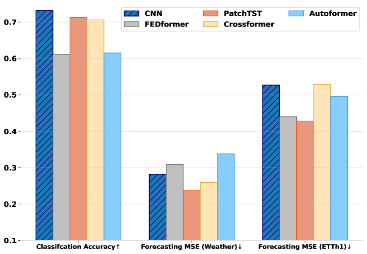
Figure 1: A comparison between CNN and Transformer-based architectures for classification and forecasting tasks. Classification results are the average over 10 UEA datasets (Wu et al., 2023), while forecasting results are the average MSE results on lengths {96, 192, 336, 720}.

Time series data, known for its sequential nature and temporal dependencies, is ubiquitous across numerous domains, including finance, healthcare, and environmental monitoring. Recently, the Transformer model (Vaswani et al., 2017), originally renowned for its breakthroughs in natural language processing, has been adapted as a potent tool for analyzing time series data. This was motivated by its ability to capture long-range dependencies and interactions within time series data, showing proficiency in forecasting tasks (Wu et al., 2021b; Zhou et al., 2022; Liu et al., 2024). Despite the initial success of Transformers in time series forecasting, they encounter hurdles when deployed across diverse time series tasks, particularly those with smaller datasets. This can be attributed to its large parameter size, which may lead to overfitting and computational inefficiency problems (Wen et al., 2023). In addition, their attention mechanism often struggles with the inherent noise and redundancy in time series data (Li et al., 2022). Moreover, recent works have questioned their adaptability, as highlighted by (Zeng et al., 2023; Li et al., 2023). They observed that the self-attention within Transformers is inherently permutation-invariant, which compromises the preservation of temporal information. Their experiments showed that a single linear layer surprisingly outperforms the complex Transformer architectures for time series forecasting. However, while such linear models can perform well for small, clean data, they may not be able to handle complex, noisy time series.

In this work, we pivot from the prevalent focus on Multi-Layer Perceptrons (MLPs) and Transformers to tackle the potential of convolutional operations for time series analysis. Convolutional Neural Networks (CNNs) have traditionally excelled in capturing short-term patterns within time series due to their local receptive fields, which serve as a strength in classification tasks. Indeed, as illustrated in Figure 1, a straightforward 3-layer CNN network demonstrates superior performance in classification compared to state-of-the-art Transformer-based architectures. Yet, our experiment showed that the efficacy of CNNs in forecasting varies with the data frequency. For instance, the CNN shows competitive performance to these Transformer-based models on the Weather dataset featuring a short 10-minute frequency but struggles with the longer hourly ETTh1 dataset, indicating a difficulty with less frequent temporal changes. This discrepancy highlights a critical question: How can we enhance CNNs to extend their robust performance across a wider spectrum of time series tasks? It becomes obvious that expanding the capabilities of CNNs can be achieved by learning both short-term and long-term dependencies within time series data.

To this end, we introduce Time Series Lightweight Adaptive Network (TSLANet), a universal architecture for various time series tasks. TSLANet inherits the multi-block design of the Transformer to allow scalability. However, we replace the computationally expensive self-attention with a lightweight Adaptive Spectral Block (ASB) featuring two key objectives. Firstly, ASB aims to encompass the entire frequency spectrum, thereby adeptly capturing both long-term and short-term interactions within the data. This is achieved via Fourier-based multiplications by global and local filters, akin to circular convolutions. Secondly, ASB selectively attenuates high frequencies via an adaptive thresholding approach, a strategy aimed at minimizing noise and enhancing the clarity of the signal. In addition, we further advance our model by replacing the standard feed-forward network with an Interactive Convolutional Block, where CNNs with different kernel sizes control each other to enrich the ability of the model to capture and interpret complex temporal patterns. Finally, we employ a per-dataset self-supervised pretraining to enhance the model capabilities, especially on large datasets.

The proposed model is lightweight and enjoys the $\mathcal{O}(N\log N)$ complexity of the Fast Fourier Transform (FFT) operations, demonstrating superior efficiency and speed compared to self-attention (see Section 5.4). A summary comparison against CNN-based and Transformer-based models is also provided in Table 1. The contributions of this paper can be summarized as follows:

• We propose a universal lightweight model (TSLANet), designed to adapt seamlessly to a myriad of time series tasks. Through computationally efficient convolution operations, TSLANet learns both long- and short-term relationships within the data.

• We propose an Adaptive Spectral Block, which leverages the power of Fourier transform alongside global and local filters to cover the whole frequency spectrum, while adaptively removing high frequencies that tend to introduce noises. In addition, we propose an Interactive Convolution Block to learn intricate spatial and temporal features within data.

• TSLANet demonstrates superior performance against different state-of-the-art methods across various time series tasks.

Table 1: Comparison to different methods. ‘Local Dependencies’ means the efficiency in capturing local features.

l—cccc Method Feature Extraction Long-range Dependencies Local Dependencies Parameter Efficiency
CNN Localized Convolution ✗ ✓ ✓
Transformer Self-Attention ✓ ✗ ✗
TSLANet Adaptive Spectral Convolution ✓ ✓ ✓

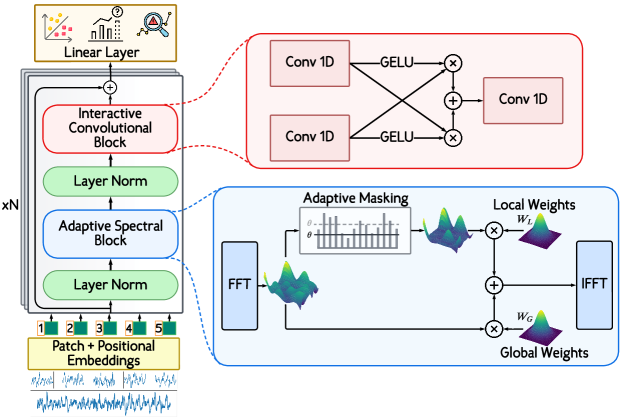
Figure 2: The structure of our proposed TSLANet. The input time series is split into patches, and positional embeddings are added. Next, the output embeddings pass through TSLANet layers, where each layer consists of two main components. The first is the Adaptive Spectral Block, which leverages frequency domain representations for robust feature extraction and employs adaptive thresholding to mitigate noise. The second is the Interactive Convolution Block, which captures complex temporal patterns through convolutional operations.

2 Related Works

Transformer-based Networks.

Since the advance of the Transformer (Vaswani et al., 2017) for natural language processing, numerous works have adopted it for time series analysis. For example, (Wu et al., 2021b; Zhou et al., 2022; Li et al., 2021; Kitaev et al., 2020; Zhang & Yan, 2023) have showcased the Transformer capability to model interactions within time series data, utilizing that for the forecasting task. In addition, Transformers with special design showed good performance in anomaly detection task (Xu et al., 2022).

Yet, the efficacy of Transformers for time series has been contested. For instance, Zeng et al. (2023) argue that the permutation-invariance property in Transformers may lead to the loss of temporal information in time series. Following that, other MLP-based architectures showed efficacy in the time series forecasting task (Li et al., 2023; Ekambaram et al., 2023). Furthermore, Transformers demand extensive computational resources in general, and they are prone to overfitting when trained on smaller datasets (Wen et al., 2023).

Convolution-based Networks.

CNNs have showcased their efficacy in time series analysis, particularly shining in classification tasks due to their adeptness at learning local patterns (Dempster et al., 2020). CNNs also serve as the backbone for several time series representation learning methods, including TS-TCC (Eldele et al., 2021), TS2VEC (Yue et al., 2022), and MHCCL (Meng et al., 2023).

Despite their promise, CNNs often face challenges in forecasting and anomaly detection, primarily due to their limited ability to capture long-range dependencies. Therefore, recent works attempt to enhance CNN capabilities in different ways. For instance, T-WaveNet (LIU et al., 2022) leverages frequency spectrum energy analysis for effective signal decomposition, SCINet (Liu et al., 2022) adopts a recursive downsample-convolve-interact strategy to model complex temporal dynamics, and WFTNet (Liu et al., 2023) employs a combination of Fourier and wavelet transforms for a thorough temporal-frequency analysis. Additionally, TCE (Zhang et al., 2023) targets the improvement of 1D-CNNs by addressing the disturbing convolution for better low-frequency component focus, and BTSF (Yang & Hong, 2022) introduces a bilinear temporal-spectral fusion technique for unsupervised learning, emphasizing the importance of maintaining the global context of time series data.

A noteworthy attempt to leverage CNNs for multiple time series tasks is the TimesNet model (Wu et al., 2023), which capitalizes on multi-periodicity to merge intraperiod and interperiod variations within a 2D space, enhancing the representation of temporal patterns. However, TimesNet may not fully address the challenges presented by non-stationary datasets lacking clear periodicity. Some recent works have explored combining CNNs with Transformers to harness both their strengths (Li et al., 2022; Wu et al., 2021a; D’Ascoli et al., 2021), though such hybrid approaches remain underexplored in time series analysis compared to their applications in computer vision.

Our work takes a distinct path by proposing a universal convolutional-based architecture, adept at handling various time series tasks through adaptive spectral feature extraction. This approach not only utilizes the strong local feature learning capabilities of CNNs but also efficiently captures global temporal patterns, offering a balanced solution for both local and long-range dependencies in time series data.

3 Method

3.1 Preliminaries: Discrete Fourier Transform

We first explore the Discrete Fourier Transform (DFT) as it is a cornerstone in our framework. Consider a series of $N$ complex numbers $x[n]$, where $0\leq n\leq N-1$. The 1D DFT transforms this series into a frequency domain representation:

$$X[k]=\sum_{n=0}^{N-1}x[n]e^{-j(2\pi/N)kn}:=\sum_{n=0}^{N-1}x[n]W_{N}^{kn},$$ (1)

where $j$ denotes the imaginary unit, with $W_{N}=e^{-j(2\pi/N)}$. This formulation is derived from the continuous Fourier transform by discretizing in both time and frequency domains. The spectrum of the sequence $x[n]$ at frequency $\omega_{k}=2\pi k/N$ is represented by $X[k]$, which is periodic with an interval of length $N$, thus only the first $N$ points are considered.

Due to the bijective nature of DFT, the original sequence $x[n]$ is retrievable via the Inverse DFT (IDFT):

$$x[n]=\frac{1}{N}\sum_{k=0}^{N-1}X[k]e^{j(2\pi/N)kn}.$$ (2)

For real-valued $x[n]$, DFT exhibits conjugate symmetry, i.e., $X[N-k]=X^{*}[k]$. This symmetry is pivotal, as performing IDFT on a conjugate symmetric $X[k]$ results in a real discrete signal. Half of the DFT spectrum, specifically ${X[k]:0\leq k\leq\lceil N/2\rceil}$, sufficiently describes the frequency characteristics of $x[n]$.

The choice of DFT in TSLANet is motivated by two factors: its discrete nature aligns well with digital processing and the existence of efficient computation methods. The Fast Fourier Transform (FFT), leveraging the symmetry and periodicity of $W_{N}^{kn}$, optimizes DFT computation from $\mathcal{O}(N^{2})$ to $\mathcal{O}(N\log N)$. The IDFT, paralleling DFT’s form, benefits similarly from the Inverse FFT (IFFT).

3.2 Overall Architecture

Our model integrates two novel components, i.e., the Adaptive Spectral Block (ASB) and the Interactive Convolution Block (ICB), as depicted in Figure 2. These two components form a single layer that could be extended to multiple layers. The ASB employs Fourier analysis to transform time series data into the frequency domain, in which we apply adaptive thresholding to attenuate high-frequency noise and highlight relevant spectral features. After processing, the IFFT reconstructs the time-domain features, now with reduced noise and enhanced representations. The ICB is a streamlined convolutional block that interactively refines features using different kernel sizes, improving adaptability to temporal dynamics in time series. Together, these components form a cohesive structure that balances local and global temporal feature extraction for time series analysis.

3.3 Embedding Layer

Given an input time series $\bm{S}$, with each signal $S\in\mathbb{R}^{C\times L}$ having $C$ channels and a sequence length $L$. First, the signal $S$ is divided into a set of $M$ patches $\{P_{1},P_{2},...,P_{M}\}$, where each patch $P_{i}$ captures a segment of $S$. The dimension of each patch is determined by the predefined patch size $p$, such that each patch $P_{i}\in\mathbb{R}^{C\times p}$.

Each patch is then mapped into another dimension $p^{\prime}$, i.e., $P_{i}\rightarrow P_{i}^{\prime}\in\mathbb{R}^{C\times p^{\prime}}$. Next, the positional embeddings are added to each patch to retain the temporal ordering disrupted during the segmentation process. The positional embedding for the $i$-th patch is denoted as $E_{i}$, a vector that aligns dimensionally with the patch. The augmented patch results from adding both inputs, i.e., $S_{PE_{i}}=P_{i}^{\prime}+E_{i}$, and $S_{PE}=\{S_{PE_{1}},S_{PE_{2}},\dots S_{PE_{M}}\}$. Notably, the positional embeddings are learnable parameters, allowing the model to capture the temporal relationships within the time series data effectively.

3.4 Adaptive Spectral Block

We propose the Adaptive Spectral Block (ASB) that employs the Fourier-domain processing, as inspired by (Rao et al., 2021). This block aims to learn spatial information with the global circular convolution operations. Moreover, it provides adaptive local filters to isolate noisy high-frequency components for any time series data.

Fast Fourier Transformations.

Given a discrete time series $x[n]$, we obtain its frequency domain representation $X[k]$, by performing FFT along the spatial dimensions as in Equation 1. Similarly, given $\bm{S_{PE}}$, its representation is calculated as:

$$\bm{F}=\mathcal{F}[\bm{S_{PE}}]\in\mathbb{C}^{C\times L^{\prime}},$$ (3)

where $\mathcal{F}[\cdot]$ denotes the 1D FFT operation, and $L^{\prime}$ is the transformed sequence length in the frequency domain, which may differ from $L$ depending on the FFT implementation and the nature of the time series data. Each channel of the time series is independently transformed, resulting in a comprehensive frequency domain representation $\bm{F}$ that encapsulates the spectral characteristics of the original time series across all channels.

Adaptive Removal of High-Frequency Noise.

High-frequency components often represent rapid fluctuations that deviate from the underlying trend or signal of interest, making them appear more random and difficult to interpret (Rhif et al., 2019). Therefore, we propose an adaptive local filter that allows the model to dynamically adjust the level of filtering according to the dataset characteristics and remove these high-frequency noisy components. This is crucial when dealing with non-stationary data, where the frequency spectrum may change over time. The proposed filter adaptively sets the appropriate frequency threshold for each specific time series data.

Given the frequency domain representation $\bm{F}$ obtained from the FFT operation, we first calculate the power spectrum of $\bm{F}$, which helps in identifying dominant frequency components. The power spectrum $\bm{P}$ is computed as the square of the magnitude of the frequency components: $\bm{P}=|\bm{F}|^{2}$, which gives us a measure of the strength of different frequencies in the time series data.

The key to effective noise reduction lies in adaptively filtering high-frequency components from the power spectrum $\bm{P}$. We achieve this with a trainable threshold $\theta$, which adjusts based on the spectral characteristics of the data. This threshold $\theta$ is set as a learnable parameter optimized during training through backpropagation, specifically $\frac{\partial\mathcal{L}}{\partial\theta}$, enabling $\theta$ to discern between essential signal frequencies and noise. We formulate this adaptive thresholding as follows:

$$\bm{F}_{\text{filtered}}=\bm{F}\odot(\bm{P}>\theta),$$ (4)

where $\odot$ represents element-wise multiplication, and $(\bm{P}>\theta)$ is a binary mask where frequencies with power above the threshold $\theta$ are retained, and others are filtered out.

The adaptability of the threshold $\theta$ ensures that the ASB can efficiently remove high frequencies while preserving crucial information. By adaptively selecting the frequency threshold, the ASB tailors its filtering process to each specific time series dataset, enhancing the overall effectiveness of the model in handling a wide range of data scenarios.

Learnable Filters.

After adaptively filtering the frequency domain data, the model employs two sets of learnable filters; a global filter to learn from the original frequency domain data $\bm{F}$ and a local filter to learn from the adaptively filtered data $\bm{F}_{\text{filtered}}$. Let $\bm{W}_{\text{G}}$ and $\bm{W}_{\text{L}}$ be the learnable global and local filters, respectively. The application of these filters is represented as:

$$\bm{F}_{\text{G}} =\bm{W}_{\text{G}}\odot\bm{F},$$ (5)

$$\bm{F}_{\text{L}} =\bm{W}_{\text{L}}\odot\bm{F}_{\text{filtered}}.$$ (6)

Next, we integrate these filtered features to capture a comprehensive spectral detail, i.e., $\bm{F}_{\text{integrated}}=\bm{F}_{\text{G}}+\bm{F}_{\text{L}}$.

Table 2: Classification results in different datasets. Results are averaged across each subset of datasets. Results are in terms of accuracy (as %). Blue: best results, Purple: second best. Full results are listed in Tables LABEL:tbl:clf_ucr_full, F.1, and 12 in the Appendix.

[b] c—ccccccccc

Methods TSLANet GPT4TS TimesNet ROCKET Crossformer PatchTST MLP TS-TCC TS2VEC
(Ours) (2023) (2023) (2020) (2023) (2023) (2023) (2021) (2022)

UCR repository (85 datasets) 83.18 61.58 65.27 81.42 73.47 71.84 69.68 75.07 81.42
UEA repository (26 datasets) 72.73 58.51 66.55 68.79 66.84 69.13 65.81 69.38 59.62
Biomedical signals (2 datasets) 90.24 87.04 87.10 87.20 70.82 83.87 70.63 92.25 86.31
Human activity recognition (3 datasets) 97.46 92.71 91.51 96.44 77.55 94.87 56.69 97.16 95.70
Average 85.90 74.96 77.61 83.46 72.17 79.93 65.70 83.55 80.76

Notably, the multiplication operations in Equations 5 and 6 are equivalent to the circular convolution process (see Appendix A). Circular convolution, with its larger receptive field over the entire sequence, is particularly adept at capturing periodic patterns in time series data.

Inverse Fourier Transform.

To convert the integrated frequency domain data back to the time domain, we apply the Inverse Fast Fourier Transform (IFFT). The resulting time-domain signal $\bm{S}^{\prime}$ is given by:

$$\bm{S}^{\prime}=\mathcal{F}^{-1}[\bm{F}_{\text{integrated}}]~{}~{}~{}~{}~{}\in\mathbb{R}^{C\times p^{\prime}}.$$ (7)

The IFFT ensures that the enhanced features align with the original data structure of the input time series. The full operation of the ASB is described in Algorithm 1 in the Appendix.

3.5 Interactive Convolution Block

After enhancing feature representation by the ASB, we propose the Interactive Convolution Block (ICB), which utilizes a dual-layer convolutional structure, as shown in Figure 2. The design of the ICB includes parallel convolutions with different kernel sizes to capture local features and longer-range dependencies. Specifically, the first convolutional layer is designed to capture fine-grained, localized patterns in the data with a smaller kernel. In contrast, the second layer aims to identify broader, longer-range dependencies with a larger kernel. We design the ICB such that the output of each layer modulates the feature extraction of the other. The element-wise multiplication encourages interactions between features extracted at different scales, potentially leading to better modeling of complex relationships.

Given the output of the IFFT operation $\bm{S}^{\prime}$, it serves as the input to the ICB. The process within the ICB is as follows:

$$\bm{A}_{1}=\phi(\text{Conv1}(\bm{S}^{\prime}))\odot\text{Conv2}(\bm{S}^{\prime}),$$ (8)

$$\bm{A}_{2}=\phi(\text{Conv2}(\bm{S}^{\prime}))\odot\text{Conv1}(\bm{S}^{\prime}),$$ (9)

where $\text{Conv1}(\cdot)$ and $\text{Conv2}(\cdot)$ are two 1D-convolutional layers and $\phi$ is the GELU activation function.

The activated features are then added and passed through a final convolutional layer $\text{Conv3}(\cdot)$:

$$\bm{O}_{\text{ICB}}=\text{Conv3}(\bm{A}_{1}+\bm{A}_{2}).$$ (10)

The output $\bm{O}_{\text{ICB}}$ represents the enhanced features ready for the final layer in the network, represented by a customizable linear layer according to the task.

3.6 Self-Supervised Pretraining

Expanding the capabilities of TSLANet, we incorporate a phase of self-supervised pretraining, which has garnered significant attention for its efficacy in learning high-level representations from unlabeled data (Nie et al., 2023). Drawing inspiration from methodologies applied in natural language processing and computer vision, we adopt a masked autoencoder paradigm for time series data (He et al., 2022).

Our implementation involves selective masking of input sequence patches, followed by training TSLANet to reconstruct these masked segments accurately. The masked data then serves as the training input, compelling the model to learn and infer the underlying patterns and dependencies in the data. Unlike methods that apply masking at individual time steps, our approach focuses on larger patches. This design choice avoids simplistic interpolation from adjacent time points and encourages the model to understand the entire sequence deeply. The reconstruction of these patches is achieved by optimizing the mean squared error (MSE) loss function.

4 Experiments

Table 3: Multivariate forecasting results with prediction lengths $\in\{96,192,336,720\}$. Results are averaged from all prediction lengths. Avg means further averaged by subsets. Blue: best results, Purple: second best. Full results are listed in Table 13 in the Appendix.

c—cc—cc—cc—cc—cc—cc—cc—cc—cc—cc—cc—cc Models TSLANet Time-LLM iTransformer

PatchTST

Crossformer

FEDformer

Autoformer

RLinear

Dlinear

TimesNet

GPT4TS

SCINet

(Ours)

(2024)

(2024)

(2023)

(2023)

(2022)

(2021b)

(2023)

(2023)

(2023)

(2023)

(2022)

Metric MSE MAE MSE MAE MSE MAE MSE MAE MSE MAE MSE MAE MSE MAE MSE MAE MSE MAE MSE MAE MSE MAE MSE MAE

ECL

0.165 0.257 0.158 0.252 0.178 0.270

0.167

0.259

0.244

0.334

0.214

0.327

0.227

0.338

0.219

0.298

0.166

0.263

0.192

0.295

0.167

0.263

0.268

0.365

ETT (Avg)

0.337 0.377 0.330 0.372 0.383 0.399

0.347

0.378

0.685

0.578

0.408

0.428

0.465

0.459

0.380

0.392

0.369

0.398

0.391

0.404

0.350

0.382

0.689

0.597

Exchange

0.369

0.404

-

-

0.360 0.403 0.367 0.404 0.940 0.707 0.519 0.429 0.613 0.539 0.378 0.417 0.297 0.378 0.416 0.443 0.370 0.406 0.750 0.626

Traffic

0.396 0.271 0.388 0.264 0.428 0.282

0.420

0.277

0.550

0.304

0.610

0.376

0.628

0.379

0.626

0.378

0.433

0.295

0.620

0.336

0.414

0.294

0.804

0.509

Weather

0.228 0.264 0.225 0.257 0.258 0.279

0.238

0.268

0.259

0.315

0.309

0.360

0.338

0.382

0.272

0.291

0.246

0.300

0.259

0.287

0.237

0.270

0.292

0.363

In this section, we evaluate the efficacy of TSLANet on time series classification, forecasting, and anomaly detection tasks. We show that our TSLANet can serve as a foundation model with competitive performance on these tasks. The detailed experimental setup is described in Section D, while the detailed experimental results are presented in Section F in the Appendix.

4.1 Classification

Datasets.

We examine the classification ability of TSLANet on a total of 116 datasets, including 85 uni-variate UCR datasets (Dau et al., 2019), 26 multi-variate UEA datasets (Bagnall et al., 2018). We also include another 5 datasets, i.e., two biomedical datasets, namely, Sleep-EDF dataset (Goldberger et al., 2000) for EEG-based sleep stage classification and MIT-BIH dataset (Moody & Mark, 2001) for ECG-based arrhythmia classification, and three human activity recognition (HAR) datasets, namely, UCIHAR (Anguita et al., 2013), WISDM (Kwapisz et al., 2011), and HHAR (Stisen et al., 2015). These datasets have different characteristics and they span a wide range of time series applications. More details about these datasets are included in Appendix E.2.

Baselines and Experimental Settings.

We select eight state-of-the-art baselines, i.e., GPT4TS (Zhou et al., 2023), TimesNet (Wu et al., 2023), ROCKET (Dempster et al., 2020), TS-TCC (Eldele et al., 2021), TS2Vec (Yue et al., 2022), Crossformer (Zhang & Yan, 2023) and PatchTST (Nie et al., 2023) as they showed the best classification accuracy over other Transformer-based architectures. Last, we experiment with a simple single-layer MLP.

Table 4: Anomaly detection task. We calculate the F1-score (as %) for each dataset. $\ast$. in the Transformers indicates the name of $\ast$former. Blue: best, Purple: second best. Table 14 in the Appendix shows the full results.

[b] Methods TSLANet GPT4TS TimesNet PatchTST ETS. FED. LightTS DLinear Stationary Auto. Pyra. Anomaly. In. Re. LogTrans. Trans. (Ours) SMD 87.91 86.89 84.61 84.62 83.13 85.08 82.53 77.10 84.72 85.11 83.04 85.49 81.65 75.32 76.21 79.56 MSL 83.32 82.45 81.84 78.70 85.03 78.57 78.95 84.88 77.50 79.05 84.86 83.31 84.06 84.40 79.57 78.68 SMAP 75.96 72.88 69.39 68.82 69.50 70.76 69.21 69.26 71.09 71.12 71.09 71.18 69.92 70.40 69.97 69.70 SWaT 92.80 94.23 93.02 85.72 84.91 93.19 93.33 87.52 79.88 92.74 91.78 83.10 81.43 82.80 80.52 80.37 PSM 97.73 97.13 97.34 96.08 91.76 97.23 97.15 93.55 97.29 93.29 82.08 79.40 77.10 73.61 76.74 76.07 Average 87.54 86.72 85.24 82.79 82.87 84.97 84.23 82.46 82.08 84.26 82.57 80.50 78.83 77.31 76.60 76.88

Results.

Table 3.4 reports the classification results, where our proposed TSLANet demonstrates superior performance over state-of-the-art baselines. Notably, convolution-based methods, including ROCKET, TS-TCC, and our approach, outperform Transformer-based models, highlighting their superiority in classification tasks. For example, in the UCR repository, TSLANet achieves an impressive accuracy of 83.18%, outperforming other models including the ROCKET, which scores 81.42%. The UEA repository results further reinforce our efficacy, with a 72.73% accuracy, compared to the next best model, PatchTST, at 69.38%. In more specialized datasets like biomedical signals and HAR, our advantage is even more pronounced, achieving an overall accuracy of 90.24% and 97.46%, respectively. These results highlight the robustness and adaptability of TSLANet in diverse time series contexts.

In our comparative analysis, Transformer models generally face challenges across various datasets, reflecting inherent limitations in handling time series data. MLP models perform well on simpler UCR datasets but falter in complex, noisy environments. TimesNet excels in datasets rich in frequency information but struggles with simpler ones. Last, the GPT4TS model shows promise in larger datasets due to the high capacity of the GPT model, yet underperforms in smaller datasets due to probable overfitting.

4.2 Forecasting

Datasets.

To assess the efficacy of TSLANet in forecasting, we conduct comprehensive evaluations on eight benchmark datasets. i.e., Electricity (ECL) featuring electricity consumption data, four ETT datasets (ETTh1, ETTh2, ETTm1, ETTm2) that encompass a range of scenarios in energy transfer technology, Exchange that encompasses fluctuating currency exchange rates, Traffic that comprises traffic flow information, and Weather that offers insights into various meteorological variables over time. We include more details about their characteristics in Appendix E.3.

Baselines and Experimental Settings.

We compare TSLANet against a variety of state-of-the-art baselines. For Transformer architectures, we compare against iTransformer (Liu et al., 2024), PatchTST, Crossformer, FEDformer (Zhou et al., 2022), and Autoformer (Wu et al., 2021b). For MLP-based models, we compare against RLinear (Li et al., 2023) and DLinear (Zeng et al., 2023) models. For general-purpose time series models, we compare our model against TimesNet and GPT4TS. For a convolutional-based forecasting model, we compare with SCINet (Liu et al., 2022). Last, we include Time-LLM (Jin et al., 2024), which is based on Large-Language Models. Similar to (Zhou et al., 2023) settings, we set the look-back window to 336 for the ETT dataset, 96 for Exchange, 512 for the Traffic and Weather datasets, and 96 for the ECL dataset. We also incorporate the data normalization block, and reverse instance norm in the forecasting task (Kim et al., 2021). For the baselines, we report the best results in their original works if they are consistent with our settings, otherwise, we re-run their codes again.

Results.

In our forecasting experiments presented in Table 4, we notice the superiority of Time-LLM due to its reliance on the large Llama-7B model (Touvron et al., 2023), which enables it to capture complex patterns and dependencies in data. Other than Time-LLM, TSLANet consistently outperforms baseline models across various datasets. Specifically, it achieves the second lowest MSE and MAE in seven out of eight datasets, showing 3% and 3.8% MSE improvement over the state-of-the-art PatchTST in ETT(avg) and Weather datasets respectively. This indicates the effectiveness of our model in handling datasets with diverse characteristics and complexities. In addition, it shows the effect of the added capability of the ASB module in learning long-range dependencies.

The results also suggest the superiority of our model over specialized Transformer-based architectures and MLP-based models. These models, e.g., iTransformer and Dlinear show competitive performance in certain datasets but fall behind in others. In addition, GPT4TS shows the power of the GPT models in the forecasting task by scoring the second-best performance in some datasets.

While Time-LLM offers slightly better performance, its computational cost is significantly higher than TSLANet. To illustrate, TSLANet demonstrates a nearly equivalent performance to Time-LLM on the ETTh1 dataset with an MSE of 0.413 compared to Time-LLM’s 0.408, yet TSLANet does so with significantly lower computational cost of 6.9e+10 FLOPS against 7.3e+12 for Time-LLM. This showcases the effective balance between performance and computational efficiency in our TSLANet.

4.3 Anomaly Detection

Datasets.

In this study, we focus on detecting anomalies in unsupervised time series data. We use five benchmark datasets for our experiments: SMD (Su et al., 2019) for server monitoring, MSL (Hundman et al., 2018) for space telemetry, SMAP (Hundman et al., 2018) for earth observations, SWaT (Mathur & Tippenhauer, 2016) for water treatment security, and PSM (Abdulaal et al., 2021) for industrial pump sensors. We discuss their details in Appendix E.4.

Baselines and Experimental Settings.

We followed the same experimental settings and adopted the same baselines in GPT4TS (Zhou et al., 2023). These are GPT4TS, TimesNet, PatchTST, ETSformer (Woo et al., 2022), FEDformer, LightTS (Zhang et al., 2022), DLinear, Stationary (Liu et al., 2022), Autoformer, Pyraformer (Liu et al., 2021), Anomalyformer (Xu et al., 2022), Informer, Reformer, LogTransformer (Li et al., 2019), and the vanilla Transformer. For data preparation, we segmented each dataset with a sliding window, following (Xu et al., 2022). We adopted the reconstruction error as our evaluation metric, common in unsupervised learning for spotting anomalies.

Results.

Table 4 presents the results, where TSLANet performs best in most of the datasets with an overall F1-score of 87.54%. It outperforms advanced models like FEDformer and Autoformer, especially in the SMD and PSM datasets with F1-scores of 87.91% and 97.73% respectively. GPT4TS model follows closely, ranking second with an overall average of 86.72%. Its high capacity makes it effective in detecting anomalies, though it slightly trails behind.

Notably, Transformer-based models exhibit lower efficacy in anomaly detection in general. This could be regarded to the attention mechanism focusing on dominant normal points, thus missing rare anomalies. Models that consider periodicity, like TimesNet and FEDformer, perform well, indicating the value of periodic analysis in highlighting unusual patterns.

Table 5: Ablation study to the effect of each component. ASB-L refers to the local filters in the ASB. UWaveGL is the UWaveGestureLibrary dataset from the UEA repository.

l—cc—cc Variant Classification (ACC %)   Forecasting (MSE)
FordA UWaveGL ETTh1 Exchange
w/o ASB 87.3 77.5 0.421 0.380
w/o ASB (L) 92.7 88.9 0.417 0.373
w/o ICB 91.3 86.2 0.419 0.376
w/o pretraining 92.5 90.6 0.415 0.372
TSLANet 93.1 91.3 0.413 0.369

5 Model Analysis

5.1 Ablation Study

In Table 4.3, we assess the contribution of the different components in our model, where we report the performance of the model when removing each component individually. Notably, removing the Adaptive Spectral Block (i.e., w/o ASB) yields a notable decline in performance. For classification tasks on FordA and UWaveGestureLibrary datasets, the accuracy drops to 87.3% and 77.5%, respectively. Similarly, its absence results in higher MSE values in the forecasting task of 0.421 and 0.380 for ETTh1 and Exchange datasets. This underscores the ASB’s critical role in feature extraction and noise reduction. Similarly, excluding the local adaptive part of the ASB (i.e., w/o ASB-L) affects the noisy datasets more than less noisy ones, highlighting the local component’s value in handling noise.

The effect of the ICB was less than the ASB, with less performance degradation in the two tasks. However, its removal shows reduced classification accuracy and increased forecasting MSE indicating its importance. The role of pretraining is similarly validated, as its absence slightly diminishes the model’s performance across both tasks.

5.2 Efficacy of Adaptive Filtering in Noise Reduction

We delve into the effectiveness of the Adaptive Filter in mitigating noise and enhancing model robustness by examining Figure 3. Specifically, Figures 2(a) and 2(b) present the performance of TSLANet, both with and without the Adaptive Filter, against the Transformer model by adding different Gaussian noise levels to the time series. The performance of the Transformer deteriorates rapidly as noise increases. In contrast, TSLANet maintains a relatively stable performance, with the variant using the Adaptive Filter showing the most resilience to noise. This is particularly noteworthy at higher noise levels, where the accuracy of the standard Transformer falls steeply, while TSLANet with the Adaptive Filter experiences a much less pronounced decline.

In Figure 2(c), we observe the frequency spectra before and after applying the Adaptive Filter. The left plot shows a noisy spectrum with high amplitude spikes across various frequencies. However, after applying the Adaptive Filter, a markedly cleaner spectrum where the amplitude of noise spikes is significantly reduced, particularly in the higher frequency range. This demonstrates the filter’s ability to attenuate unwanted noise while preserving the relevant signal.

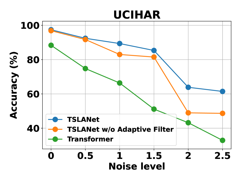
(a) Robustness against noise levels on UCIHAR dataset.

(b) Robustness against noise levels on NATOPS dataset.

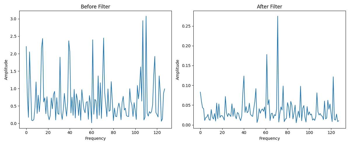
(c) The features before and after the local adaptive filter on the UEA Handwriting dataset.

Figure 3: Effectiveness of the Adaptive Filter in noise reduction.

5.3 Scaling Efficiency

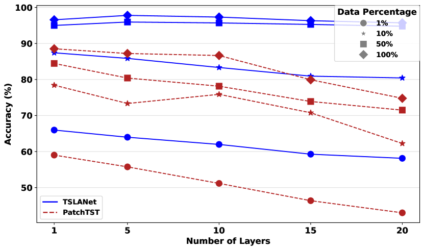
Figure 4: A comparison between TSLANet vs. PatchTST in terms of accuracy with varying the number of layers in both for different data percentages from the uWaveGestureLibraryAll dataset.

We compare the scalability of our TSLANet with one of the best-performing Transformer models in the classification task, i.e., PatchTST (Nie et al., 2023), by observing their performance across various dataset sizes and layer counts. Specifically, we experiment with variable data sizes from the uWaveGestureLibraryAll dataset, as shown in Figure 4. Notably, in smaller data sizes, TSLANet demonstrates a consistent accuracy level, subtly decreasing as the number of layers increases. In contrast, the PatchTST shows a marked decline in accuracy with additional layers, suggesting a potential overfitting issue or inefficiency in handling limited data with increased model complexity.

As dataset sizes grow, TSLANet performance remains robust, showing slight variations in accuracy with more layers. This stability contrasts with the PatchTST performance, which tends to decrease notably at higher layer counts. This trend in PatchTST could be attributed to their inherent design, which might lead to diminishing returns or optimization challenges as the model depth increases. Lastly, we notice that TSLANet effectively leverages larger dataset samples, as its performance improves with an increase in the number of layers, highlighting its capacity to capitalize on more extensive data for enhanced accuracy.

5.4 Complexity Analysis

We compare the complexity of our TSLANet with TimesNet and Transformer-based models, e.g., PatchTST, FEDFormer, AutoFormer, Informer, and Reformer in terms of the number of parameters, FLOPs, and accuracy on the UEA Heartbeat dataset, as shown in Figure 5. TSLANet demonstrates superior efficiency and accuracy in time series analysis, achieving the highest accuracy of 77.56% with the lowest computational and parameter footprint among the compared models. It requires 93% fewer FLOPs and 84% fewer parameters than the PatchTST, yet outperforms it by over 8% in accuracy. Compared to TimesNet, TSLANet operates with more than 99% fewer FLOPs and parameters while still delivering a 3% higher accuracy.

This considerable reduction in computational demand confirms the lightweight nature of TSLANet compared to Transformer-based alternatives, underscoring its capacity to make time series analysis more efficient.

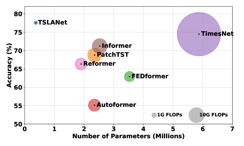
Figure 5: TSLANet vs. baselines in terms of the number of parameters and FLOPS count against the classification accuracy of the UEA Heartbeat dataset.

6 Conclusions

In this paper, we introduced TSLANet, a novel lightweight model for time series analysis that revisits the convolution approach as a potent replacement to Transformers, with an innovative combination of convolution operations and adaptive spectral analysis. Our comprehensive experiments across various datasets in classification, forecasting, and anomaly detection have demonstrated its superior performance over traditional Transformer models, particularly in its ability to maintain high accuracy levels in noisy conditions and across different data sizes. Furthermore, our in-depth layer-wise performance analysis revealed that TSLANet not only outperforms Transformers in smaller datasets but also exhibits improved scalability with increasing layers, particularly in larger datasets. TSLANet is a step towards a foundation model for time series analysis.

Impact Statement

Our proposed work TSLANet aims to advance the field of Machine Learning by providing a more efficient, scalable, and robust foundation model for analyzing time series data across various applications. It has the potential to impact various sectors, including healthcare, finance, and environmental monitoring, by enhancing forecasting accuracy and anomaly detection capabilities. Such improvements could lead to better patient outcomes, more informed financial decisions, and greater preparedness for natural disasters.

Appendix A Circular Convolutions

The convolution theorem suggests that the multiplication in the frequency domain is equivalent to the circular convolution process.

Let $x[n]$ and $h[n]$ be two length $N$ sequences. Their DFTs are $X[k]$ and $H[k]$, respectively. Consider the circular convolution $y[n]=(x\circledast h)[n]$. The DFT of $y[n]$ is $Y[k]$.

First, the DFT of the Convolution can be formulated as:

$$Y[k]=\sum_{n=0}^{N-1}\left(\sum_{m=0}^{N-1}x[m]\cdot h[(n-m)\mod N]\right)\cdot e^{-i2\pi kn/N}$$

However, if we changed the order of summation, it becomes:

$$Y[k]=\sum_{m=0}^{N-1}x[m]\cdot\sum_{n=0}^{N-1}h[(n-m)\mod N]\cdot e^{-i2\pi kn/N}$$

By substituting $n-m$ with $r$:

$$Y[k]=\sum_{m=0}^{N-1}x[m]\cdot e^{-i2\pi km/N}\cdot\sum_{r=0}^{N-1}h[r]\cdot e^{-i2\pi kr/N}$$

Therefore, we recognize the DFTs of $x[n]$ and $h[n]$:

$$Y[k]=\left(\sum_{m=0}^{N-1}x[m]\cdot e^{-i2\pi km/N}\right)\cdot\left(\sum_{r=0}^{N-1}h[r]\cdot e^{-i2\pi kr/N}\right)$$

$$Y[k]=X[k]\cdot H[k]$$

Thus, we have shown that the DFT of the circular convolution of two sequences $x[n]$ and $h[n]$ is the product of their individual DFTs, i.e., $Y[k]=X[k]\cdot H[k]$.

Appendix B Frequency Domain Processing Role to Learn Long-Range Dependencies

Fourier transforms, used in our Adaptive Spectral Block (ASB), can learn long-range and short-range dependencies in time series. The Fourier Transform (FT) of a time series $x(t)$ is given by:

$$X(f)=\int_{-\infty}^{\infty}x(t)e^{-j2\pi ft}dt$$

where $X(f)$ represents the signal in the frequency domain, $f$ is the frequency, and $t$ represents time.

The FT decomposes $x(t)$ into its constituent frequencies, where each frequency component represents a pattern in the time series. Low-frequency components correspond to long-range dependencies (slowly changing trends), and high-frequency components correspond to short-range dependencies (rapid fluctuations). Let’s consider a simplified model where the ASB applies a filter $H(f)$ to the Fourier transform $X(f)$ of the input signal, enhancing certain frequencies while attenuating others:

$$Y(f)=H(f)\cdot X(f)$$

where $Y(f)$ is the output signal in the frequency domain.

The adaptiveness comes from adjusting $H(f)$ based on the data, which can be modeled as a learning process where $H(f)$ is updated to minimize a loss function $L$ that measures the discrepancy between the model output and the true data characteristics:

$$\min_{H(f)}L(Y(f),\text{True Data})$$

Through this process, $H(f)$ learns to emphasize the frequency components that are most relevant for predicting the target, whether they capture long-range or short-range dependencies.

After filtering in the frequency domain, the inverse Fourier transform (IFT) is applied to convert $Y(f)$ back into the time domain, yielding the modified signal $y(t)$:

$$y(t)=\int_{-\infty}^{\infty}Y(f)e^{j2\pi ft}df$$

This signal now encapsulates the learned dependencies, ready for further processing or as an input to subsequent model layers.

Appendix C Algorithm of Adaptive Spectral Block

Algorithm 1 Pseudocode of the Adaptive Spectral Block.

⬇

def adaptive_high_freq_mask(x, threshold):

# Calculate energy

energy = torch.abs(x_fft).pow(2).sum(dim=-1)

# Compute the adaptive threshold

threshold = torch.quantile(energy, threshold)

# Identify the dominant frequencies

dominant_freq = normalized_energy > threshold

# Set adaptive mask values

adaptive_mask[dominant_freq] = 1

return adaptive_mask

# Transform input x_in to frequency domain

X_fft = fft(x_in)

# Create an adaptive mask for high-freq. components

freq_mask = adaptive_high_freq_mask(X_fft, threshold)

# Apply adaptive high-frequency mask

X_masked = X_fft * freq_mask

# Apply global and local learnable weights

X_L = X_masked * local_weight

X_G = X_fft * global_weight

# Transform data back into the time domain

x_out = ifft(X_L + X_G)

Appendix D Experimental Setup

D.1 Training Protocol

To train the classification experiments, we optimized TSLANet using AdamW with a learning rate of 1e-3 and a weight decay of 1e-4, applied during both training and pretraining phases. The experiments ran for 50 epochs for pretraining and 100 epochs for fine-tuning. For the forecasting and anomaly detection experiments, we utilized a learning rate of 1e-4 and a weight decay of 1e-6, with both phases running for 10 epochs.

For all experiments, the patch size was set to 8 and the stride to 4. Each experiment was repeated three times, with the average performance reported. TSLANet was implemented using PyTorch and conducted on NVIDIA RTX A6000 GPUs.

D.2 Objective Functions

For the classification task, we employ a categorical cross-entropy loss function with label smoothing, defined as $\mathcal{L}_{\text{clf}}=-\sum_{i=1}^{C}y_{i}^{\text{smooth}}\cdot\log(\hat{y}_{i})$. Here, $y_{i}^{\text{smooth}}$ is the true class label in one-hot encoded form adjusted via label smoothing, $\hat{y}_{i}$ is the predicted probability for each class, and $C$ is the total number of classes. Label smoothing reduces model confidence by adjusting the true labels with a smoothing parameter $\epsilon$, making the distribution more uniform, where each $y_{i}$ is transformed to $y_{i}^{\text{smooth}}=(1-\epsilon)\cdot y_{i}+\frac{\epsilon}{C}$.

In forecasting and anomaly detection, we use the Mean Squared Error (MSE) to measure discrepancies between predicted values and actual observations, expressed as $\mathcal{L}_{\text{MSE}}=\frac{1}{N}\sum_{i=1}^{N}(y_{i}-\hat{y}_{i})^{2}$. Here, $y_{i}$ represents the actual value at time $i$, $\hat{y}_{i}$ denotes the forecasted value, and $N$ is the number of predictions. This MSE loss is also utilized in self-supervised learning tasks to reconstruct masked patches.

D.3 Evaluation Metrics

Model performance was evaluated using standard metrics appropriate to each task. For classification, we reported accuracy; for forecasting, Mean Squared Error (MSE) and Mean Absolute Error (MAE) were used; for anomaly detection, the F1-score was our primary metric due to the imbalanced nature of the datasets.

Appendix E Datasets Details

E.1 Data Preprocessing

For the classification task, the UCR and UEA datasets are already split into train/test splits. A validation set was picked from each dataset in the training set with a ratio of 80/20. The selection of the hyperparameters was based on the average results on the validation sets across each collection of datasets, i.e., UCR and UEA. For biomedical and human activity recognition datasets, which are not split by default, we split the data into a 60/20/20 ratio for train/validation/test splits. For forecasting and anomaly detection datasets, these are split into a ratio of 70/10/20 following a line of previous works, towards a fair comparison with these works (Zhou et al., 2022; Kitaev et al., 2020; Li et al., 2021; Wu et al., 2023). All datasets are normalized during training.

For the self-supervised task, we deploy the unlabeled version of the training set in each dataset for pretraining, then use the same set again with labels for fine-tuning.

E.2 Classification

In our evaluation, we extensively utilize four categories of datasets:

• UCR datasets: The UCR Time Series Classification Archive is one of the most comprehensive collections of univariate datasets tailored for time series analysis. This archive encompasses 85 diverse datasets, each presenting unique challenges and characteristics that span a wide array of domains, from healthcare and finance to environmental monitoring and beyond. The variety within the UCR archive allows for a robust assessment of TSLANet across different contexts, showcasing its versatility and performance.

• UEA datasets: We also incorporate datasets from the University of East Anglia (UEA) Time Series Classification repository, which is renowned for its rich collection of multivariate time series datasets. We were able to preprocess 26 datasets, each offering a multidimensional perspective on time series analysis across various real-world scenarios, such as human activity recognition, sensor data interpretation, and complex system monitoring. More details about the UCR and UEA datasets can be found in https://www.timeseriesclassification.com/.

• Biomedical datasets: The biomedical domain presents unique challenges and opportunities for time series analysis. In this context, we utilized two pivotal datasets for our evaluation: the Sleep-EDF dataset and the MIT-BIH Arrhythmia dataset.

  • Sleep-EDF Dataset: This dataset consists of polysomnography recordings intended for sleep stage classification. It is part of the PhysioNet database and includes polysomnographic sleep recordings that have been widely used to analyze sleep patterns and stages. For our analysis, we extracted the brain EEG signals.

  • MIT-BIH Arrhythmia Dataset: Another significant dataset from PhysioNet, the MIT-BIH Arrhythmia Dataset, is composed of electrocardiogram (ECG) recordings used primarily for arrhythmia detection and classification. It is one of the most extensively used datasets for validating arrhythmia detection algorithms, offering a comprehensive collection of annotated heartbeats and arrhythmia examples.

  A summary of the characteristics of these two datasets is presented in Table 6.

• Human Activity Recognition datasets: Human activity recognition (HAR) using sensor data is a vital application of time series analysis, with implications for health monitoring, elder care, and fitness tracking. In this study, we evaluate our model using three prominent HAR datasets: UCIHAR, WISDM, and HHAR.

  • UCI Human Activity Recognition Using Smartphones (UCIHAR): This dataset is collected from experiments that were carried out with a group of 30 volunteers performing six activities (walking, walking upstairs, walking downstairs, sitting, standing, and laying) while wearing a smartphone on the waist. The smartphone’s embedded accelerometer and gyroscope captured 3-axial linear acceleration and 3-axial angular velocity, respectively.

  • Wireless Sensor Data Mining (WISDM): The WISDM dataset includes time series data from smartphone sensors and wearable devices, capturing various human activities such as walking, jogging, sitting, and standing. It provides a diverse set of user-generated activity data, making it suitable for testing the robustness of HAR models across different motion patterns and sensor placements.

  • Heterogeneity Human Activity Recognition (HHAR): HHAR dataset stands out due to its collection from multiple device types, including smartphones and smartwatches, across different individuals performing activities like biking, sitting, standing, walking, stair climbing, and more. Its heterogeneity in terms of device types and positions offers a challenging benchmark for assessing a model’s ability to generalize across various sensor configurations and activity types. Here, we utilized the data from the Samsung devices.

  A summary of the characteristics of these three datasets is presented in Table 7.

Table 6: A description of characteristics of the biomedical datasets used in our experiments.

Dataset	# Train	# Test	Length	# Channel	# Class
Sleep EEG	25,612	8,910	3,000	2	5
Arrhythmia ECG	70,043	21,892	187	1	2

Table 7: A description of characteristics of the Human Activity Recognition datasets used in our experiments.

Dataset	# Train	# Test	Length	# Channel	# Class
UCIHAR	7,352	2,947	128	9	6
WISDM	4,731	2,561	128	3	6
HHAR	10,336	4,436	128	3	6

E.3 Forecasting

Our study leverages a diverse set of forecasting datasets to evaluate the effectiveness of our model across various domains:

• Electricity: This dataset contains electricity consumption records from 321 clients, offering insights into usage patterns and enabling demand forecasting, crucial for optimizing power generation and distribution.

• ETT (Electricity Transformer Temperature) datasets: The ETTh1, ETTh2, ETTm1, and ETTm2 datasets provide data on the temperature of electricity transformers and the load, facilitating the prediction of future temperatures and loads based on past patterns. These datasets vary in granularity, with ”h” indicating hourly data and ”m” indicating 15-minute intervals, offering a range of temporal resolutions for forecasting challenges.

• Exchange Rate: Featuring daily exchange rates of different currencies against the US dollar, this dataset is vital for financial forecasting, enabling models to anticipate currency fluctuations based on historical data.

• Traffic: Traffic dataset consists of hourly interstate 94 Westbound traffic volume for the Twin Cities (Minneapolis-St. Paul) metropolitan area, allowing for the prediction of traffic flow patterns, essential for urban planning and congestion management.

• Weather: This dataset includes hourly weather conditions and atmospheric measurements from a weather station, supporting forecasts of various weather phenomena, crucial for agriculture, transportation, and daily life planning.

We describe the characteristics of these datasets in Table 8.

Table 8: Descriptions of the forecasting datasets. Dim shows the variate number of each dataset. Dataset Size indicates the size of the (Train, Validation, Test) split respectively. Frequency denotes the sampling interval of time points.

Dataset	Dim	Dataset Size	Frequency	Information
ECL	321	(18317, 2633, 5261)	Hourly	Electricity
ETTh1, ETTh2	7	(8545, 2881, 2881)	Hourly	Electricity
ETTm1, ETTm2	7	(34465, 11521, 11521)	15min	Electricity
Exchange	8	(5120, 665, 1422)	Daily	Economy
Traffic	862	(12185, 1757, 3509)	Hourly	Transportation
Weather	21	(36792, 5271, 10540)	10min	Weather

E.4 Anomaly Detection

Anomaly detection plays a pivotal role across various domains, enabling the identification of unusual patterns that may indicate critical incidents, such as system failures, security breaches, or environmental changes. In our study, we assess the performance of our model using five benchmark datasets, each representing a distinct application area, to demonstrate its effectiveness in detecting anomalies in diverse settings:

• SMD (Server Machine Dataset): Utilized for server monitoring, the SMD dataset comprises multivariate time series data collected from servers and aims to identify unusual server behaviors that could indicate failures or security issues.

• MSL (Mars Science Laboratory): This dataset contains telemetry data from the Mars Science Laboratory rover, focusing on space exploration applications. Anomaly detection in this context is crucial for identifying potential issues with spacecraft systems based on their operational data.

• SMAP (Soil Moisture Active Passive): Related to earth observations, the SMAP dataset includes soil moisture measurements intended for environmental monitoring. Detecting anomalies in soil moisture can provide insights into environmental conditions and potential agricultural impacts.

• SWaT (Secure Water Treatment): In the domain of water treatment security, the SWaT dataset consists of data from a water treatment testbed, simulating the operational data of water treatment plants. Anomaly detection here is vital for ensuring the safety and security of water treatment processes.

• PSM (Pump Sensor Monitoring): Focused on industrial pump sensors, the PSM dataset gathers sensor data from pumps in industrial settings. Anomalies in this dataset can indicate equipment malfunctions or the need for maintenance, critical for preventing industrial accidents.

The detailed characteristics of these datasets is presented in Table 9.

Table 9: Descriptions of the Anomaly detection datasets. Dim shows the variate number of each dataset. Dataset Size indicates the size of the (Train, Validation, Test) split respectively. Frequency denotes the sampling interval of time points.

Dataset	Dim	Length	Dataset Size	Information
SMD	38	100	(566724, 141681, 708420)	Server Machine
MSL	55	100	(44653, 11664, 73729)	Spacecraft
SMAP	25	100	(108146, 27037, 427617)	Spacecraft
SWaT	51	100	(396000, 99000, 449919)	Infrastructure
PSM	25	100	(105984, 26497, 87841)	Server Machine

Appendix F Full Results

F.1 Classification

Table 10: Full classification results on the UCR datasets in terms of accuracy (as %).

Dataset	TSLANet	GPT4TS	TimesNet	ROCKET	CrossF.	Pat.TST	MLP	TS-TCC	TS2VEC
Adiac	80.56	52.69	24.04	78.52	58.31	34.78	61.38	76.57	72.89
ArrowHead	80.57	66.29	49.71	77.31	73.71	72.57	75.43	62.20	77.71
Beef	90.00	66.67	60.00	67.33	73.33	76.67	73.33	47.32	76.67
BeetleFly	90.00	85.00	80.00	88.00	85.00	80.00	80.00	31.25	85.00
BirdChicken	100.00	85.00	60.00	84.50	85.00	80.00	75.00	75.00	80.00
CBF	97.56	92.00	92.22	89.67	89.56	85.11	83.44	90.79	88.33
Car	88.33	76.67	30.00	99.52	86.67	75.00	86.67	71.88	99.22
ChlorineConcentration	85.94	61.25	55.21	69.40	61.72	56.56	61.72	57.40	71.85
CinC_ECG_torso	85.51	23.99	51.74	84.96	84.93	66.88	46.67	95.55	79.28
Coffee	100.00	100.00	53.57	100.00	100.00	100.00	100.00	95.83	100.00
Computers	68.40	52.00	62.40	66.48	63.20	69.60	58.00	61.95	60.40
Cricket_X	76.15	6.41	55.64	77.31	41.79	45.38	32.56	77.25	76.15
Cricket_Y	78.72	49.74	55.90	79.15	47.69	43.59	42.31	75.75	73.08
Cricket_Z	80.00	8.21	57.44	79.33	41.79	47.95	32.56	75.83	76.92
DiatomSizeReduction	92.16	88.89	48.69	97.68	95.75	91.18	93.14	95.94	97.71
DistalPhalanxOutlineAgeGroup	86.50	86.50	80.25	76.12	80.75	82.00	80.50	85.25	81.25
DistalPhalanxOutlineCorrect	80.67	75.67	73.67	75.68	76.17	78.50	75.50	80.76	81.17
DistalPhalanxTW	80.50	78.25	77.25	70.07	79.25	79.00	79.50	79.50	78.00
Earthquakes	82.30	38.82	23.60	75.32	82.30	80.75	59.94	75.89	72.36
ECG200	88.00	85.00	90.00	84.90	86.00	89.00	84.00	87.50	87.00
ECG5000	94.62	93.40	93.47	94.72	94.36	93.87	94.18	94.19	93.33
ECGFiveDays	99.30	94.77	83.74	100.00	98.49	86.41	96.63	90.71	100.00
ElectricDevices	68.28	56.36	68.58	66.84	61.87	74.66	48.22	69.31	68.10
FaceAll	82.31	37.22	73.61	93.33	90.53	79.94	78.64	76.99	79.17
FaceFour	94.32	7.95	52.27	77.39	93.18	86.36	82.95	85.42	94.32
FacesUCR	92.39	82.88	46.00	94.81	83.07	77.46	74.39	92.93	94.24
FiftyWords	80.00	36.48	61.32	76.92	62.86	55.16	58.90	77.62	79.12
FISH	94.29	71.43	59.43	96.86	84.57	71.43	87.43	61.29	93.14
FordA	93.06	50.49	66.20	90.61	70.62	50.90	51.32	92.35	89.28
FordB	91.39	61.99	54.43	77.53	52.70	52.20	51.16	91.72	83.50
Gun_Point	99.33	90.00	87.33	99.33	89.33	94.00	85.33	93.33	98.00
Ham	80.00	51.43	65.71	69.43	78.10	73.33	77.14	75.00	72.38
HandOutlines	88.90	36.20	86.30	94.35	86.00	85.20	86.40	85.81	85.70
Haptics	47.73	26.95	37.01	50.84	43.83	41.23	46.10	44.06	43.51
Herring	67.19	40.63	59.38	64.38	68.75	64.06	70.31	60.94	64.06
InlineSkate	36.73	18.91	25.82	39.64	30.91	29.45	27.82	29.76	38.55
InsectWingbeatSound	66.36	63.23	60.00	63.92	64.29	57.83	64.75	66.52	63.79
ItalyPowerDemand	97.08	96.89	97.08	97.17	97.28	96.60	96.89	96.44	95.63
LargeKitchenAppliances	81.87	33.33	47.20	81.47	53.87	63.20	42.13	76.08	86.40
Lighting2	83.61	54.10	72.13	73.61	75.41	75.41	67.21	73.56	86.89
Lighting7	83.56	53.42	72.60	68.63	72.60	67.12	64.38	81.53	83.56
MALLAT	94.71	91.86	54.50	94.12	93.48	84.01	95.05	91.11	89.13
Meat	93.33	50.00	33.33	93.33	88.33	91.67	80.00	31.25	91.67
MedicalImages	72.76	61.18	58.95	75.42	65.79	63.03	59.61	74.35	75.79
MiddlePhalanxOutlineAgeGroup	81.25	74.50	78.75	83.64	80.75	79.75	80.75	78.25	75.25
MiddlePhalanxOutlineCorrect	84.00	64.67	64.67	61.36	64.50	64.83	64.50	52.47	71.67
MiddlePhalanxTW	65.91	64.91	64.66	53.77	64.66	64.16	65.16	56.10	61.65
MoteStrain	93.13	87.14	88.34	83.49	87.22	89.54	86.74	85.28	87.86
NonInvasiveFatalECG_Thorax1	93.44	72.98	81.58	95.65	86.97	78.73	92.98	84.58	90.48
NonInvasiveFatalECG_Thorax2	93.74	88.04	84.38	95.59	90.53	85.24	93.49	82.50	93.74
OliveOil	40.00	40.00	40.00	80.33	60.00	83.33	70.00	42.86	90.00
OSULeaf	74.79	9.50	43.39	82.89	49.59	42.15	45.04	63.28	76.86
PhalangesOutlinesCorrect	82.40	77.04	68.30	83.11	69.35	65.97	66.90	78.73	80.77
Phoneme	27.27	3.22	9.70	20.92	11.23	9.12	8.60	30.04	26.79
Plane	100.00	97.14	98.10	100.00	98.10	99.05	97.14	96.43	100.00
ProximalPhalanxOutlineAgeGroup	88.29	83.90	86.34	90.17	86.34	86.34	85.85	73.34	81.95
ProximalPhalanxOutlineCorrect	91.75	81.79	77.66	86.59	84.54	78.01	81.79	87.17	87.29
ProximalPhalanxTW	83.00	81.50	81.75	78.98	80.00	80.25	82.75	72.75	79.00
RefrigerationDevices	55.47	33.60	33.60	50.40	42.40	45.87	38.67	49.74	51.20
ScreenType	44.80	37.07	44.00	41.55	45.07	44.80	40.27	39.99	40.00
ShapeletSim	90.00	49.44	50.00	65.72	57.22	56.67	56.67	61.98	87.78
ShapesAll	85.17	61.17	64.33	86.63	68.17	61.00	61.83	79.11	88.00
SmallKitchenAppliances	76.27	33.33	45.60	62.13	55.47	61.60	41.33	74.74	71.20
SonyAIBORobotSurface	85.86	42.93	70.55	93.16	81.03	83.69	70.38	68.46	89.18
SonyAIBORobotSurfaceII	92.44	70.30	85.62	91.26	85.73	85.73	85.10	86.15	90.66
StarLightCurves	97.41	92.70	89.22	97.63	92.74	86.09	91.96	96.80	96.28
Strawberry	98.37	94.94	93.15	97.84	94.45	93.15	95.76	93.59	96.57
SwedishLeaf	96.16	88.32	83.40	96.10	82.08	76.64	80.96	92.31	93.60
Symbols	94.07	16.98	86.43	96.71	86.13	82.21	84.72	86.08	96.58
Synthetic_control	100.00	97.67	99.67	99.53	93.67	99.67	87.00	99.67	99.67
ToeSegmentation1	87.72	52.63	61.40	94.21	62.28	66.23	60.09	78.75	92.11
ToeSegmentation2	90.00	75.38	86.15	91.00	81.54	76.92	58.46	59.72	87.69
Trace	100.00	68.00	66.00	100.00	74.00	100.00	67.00	97.32	100.00
TwoLeadECG	93.85	76.56	68.74	100.00	86.65	84.55	91.48	81.63	99.78
Two_Patterns	100.00	99.58	98.00	100.00	79.90	93.23	84.13	100.00	99.21
uWaveGestureLibrary_X	82.80	69.65	69.37	82.64	66.78	65.02	64.77	80.97	77.89
uWaveGestureLibrary_Y	73.53	54.22	62.67	73.83	61.33	55.11	60.19	71.22	67.87
uWaveGestureLibrary_Z	75.15	59.27	60.44	75.05	59.35	55.05	56.98	72.92	72.67
uWaveGestureLibraryAll	97.57	85.54	90.28	97.20	88.02	87.58	88.22	96.54	91.99
wafer	99.81	99.58	99.71	99.84	98.39	99.63	94.78	99.69	99.85
Wine	66.67	53.70	50.00	71.30	68.52	77.78	72.22	57.81	85.19
WordsSynonyms	69.28	7.37	50.16	71.30	56.90	49.06	44.83	66.12	68.81
Worms	60.77	17.68	43.65	65.97	34.25	34.81	31.49	51.98	55.80
WormsTwoClass	77.35	58.01	62.98	76.62	62.43	60.77	58.01	64.48	69.61
yoga	85.83	71.83	67.77	90.49	73.87	68.43	65.13	77.46	84.23
Average	83.18	61.58	65.27	81.42	73.47	71.84	69.68	75.07	81.42
1st count	38	0	1	27	2	2	2	4	9

Table 11: Full classification results on the UEA datasets in terms of accuracy (as %).

l—c—c—c—c—c—c—c—c—c Dataset TSLANet GPT4TS TimesNet ROCKET CrossF. PatchTST MLP TS-TCC TS2VEC

ArticularyWordRecognition 99.00 93.33 96.18 99.33 98.00 97.67 97.33 98.00 87.33
AtrialFibrillation 40.00 33.33 33.33 20.00 46.66 53.33 46.66 33.33 53.33
BasicMotions 100.00 92.50 100.00 100.00 90.00 92.50 85.00 100.00 92.50
Cricket 98.61 8.33 87.50 98.61 84.72 84.72 91.67 93.06 65.28
Epilepsy 98.55 85.51 78.13 98.55 73.19 65.94 60.14 97.10 62.32
EthanolConcentration 30.42 25.48 27.73 42.58 34.98 28.90 33.46 32.32 40.68
FaceDetection 66.77 65.58 67.47 64.70 66.17 68.96 67.42 63.05 50.96
FingerMovements 61.00 57.00 59.38 61.00 64.00 62.00 64.00 44.00 51.00
HandMovementDirection 52.70 18.92 50.00 50.00 58.11 58.11 58.11 64.86 32.43
Handwriting 57.88 3.76 26.18 48.47 26.24 26.00 22.47 47.76 15.53
Heartbeat 77.56 36.59 74.48 69.76 76.59 76.59 73.17 77.07 69.76
InsectWingbeat 10.00 10.00 10.00 10.00 10.00 10.00 10.00 10.00 10.00
JapaneseVowels 99.19 98.11 97.83 95.68 98.92 98.65 97.84 97.30 90.00
Libras 92.78 79.44 77.84 83.89 76.11 81.11 73.33 86.67 85.56
LSST 66.34 46.39 59.21 54.10 42.82 67.80 35.77 49.23 39.01
MotorImagery 62.00 50.00 51.04 53.00 61.00 61.00 61.00 47.00 47.00
NATOPS 95.56 91.67 81.82 83.33 88.33 96.67 93.89 96.11 82.22
PEMS-SF 83.82 87.28 88.13 75.10 82.08 88.44 82.08 86.71 72.25
PenDigits 98.94 97.74 98.19 97.34 93.65 99.23 92.94 98.51 97.40
PhonemeSpectra 17.75 3.01 18.24 17.60 7.55 11.69 7.10 25.92 8.23
RacketSports 90.79 76.97 82.64 86.18 81.58 84.21 78.95 84.87 74.34
SelfRegulationSCP1 91.81 91.47 77.43 84.64 92.49 89.76 88.40 91.13 77.13
SelfRegulationSCP2 61.67 51.67 52.84 54.44 53.33 54.44 51.67 53.89 51.11
SpokenArabicDigits 99.91 99.36 98.36 99.20 96.41 99.68 96.68 99.77 85.27
StandWalkJump 46.67 33.33 53.33 46.67 53.33 60.00 60.00 40.00 46.67
UWaveGestureLibrary 91.25 84.38 83.13 94.40 81.56 80.00 81.88 86.25 62.81
Average 72.73 58.51 66.55 68.79 66.84 69.13 65.81 69.38 59.62
1st count 12 0 0 3 2 7 0 2 0

Table 12: Full classification results on the human activity recognition and biomedical signal datasets in terms of accuracy (as %).

Dataset	TSLANet	GPT4TS	TimesNet	ROCKET	CrossF.	PatchTST	MLP	TS-TCC	TS2VEC
UCIHAR	96.06	91.24	91.34	94.37	76.59	92.70	63.49	95.95	96.19
WISDM	97.77	89.49	89.61	97.03	77.31	95.94	58.88	97.05	93.87
HHAR	98.53	97.40	93.59	97.93	78.74	95.96	47.70	98.49	97.05
Average	97.46	92.71	91.51	96.44	77.55	94.87	56.69	97.16	95.70
EEG	82.10	76.37	75.86	76.69	53.30	69.69	49.70	86.06	75.13
ECG	98.37	97.70	98.33	97.72	88.33	98.06	91.57	98.44	97.48
Average	90.24	87.04	87.10	87.20	70.82	83.87	70.63	92.25	86.31

F.2 Forecasting

Table 13: Full forecasting results on different prediction lengths $\in\{96,192,336,720\}$. Lower MSE indicates better performance.

Methods		TSLANet		Time-LLM		iTransformer		PatchTST		Crossformer		FEDformer		Autoformer		RLinear		Dlinear		TimesNet		GPT4TS		SCINet
Metric		MSE	MAE	MSE	MAE	MSE	MAE	MSE	MAE	MSE	MAE	MSE	MAE	MSE	MAE	MSE	MAE	MSE	MAE	MSE	MAE	MSE	MAE	MSE	MAE
$ECL$	96	0.136	0.229	0.131	0.224	0.148	0.240	0.138	0.230	0.219	0.314	0.193	0.308	0.201	0.317	0.201	0.281	0.140	0.237	0.168	0.272	0.139	0.238	0.247	0.345
	192	0.152	0.244	0.152	0.241	0.162	0.253	0.149	0.243	0.231	0.322	0.201	0.315	0.222	0.334	0.201	0.283	0.153	0.249	0.184	0.289	0.153	0.251	0.257	0.355
	336	0.168	0.262	0.160	0.248	0.178	0.269	0.169	0.262	0.246	0.337	0.214	0.329	0.231	0.338	0.215	0.298	0.169	0.267	0.198	0.300	0.169	0.266	0.269	0.369
	720	0.205	0.293	0.192	0.298	0.225	0.317	0.211	0.299	0.280	0.363	0.246	0.355	0.254	0.361	0.257	0.331	0.203	0.301	0.220	0.320	0.206	0.297	0.299	0.390
	Avg	0.165	0.257	0.158	0.252	0.178	0.270	0.167	0.259	0.244	0.334	0.214	0.327	0.227	0.338	0.219	0.298	0.166	0.264	0.193	0.295	0.167	0.263	0.268	0.365
$ETTh1$	96	0.370	0.394	0.362	0.392	0.386	0.405	0.382	0.401	0.423	0.448	0.376	0.419	0.449	0.459	0.386	0.395	0.375	0.399	0.384	0.402	0.376	0.397	0.654	0.599
	192	0.412	0.417	0.398	0.418	0.441	0.436	0.428	0.425	0.471	0.474	0.420	0.448	0.500	0.482	0.437	0.424	0.405	0.416	0.436	0.429	0.416	0.418	0.719	0.631
	336	0.399	0.416	0.430	0.427	0.487	0.458	0.451	0.436	0.570	0.546	0.459	0.465	0.521	0.496	0.479	0.446	0.439	0.443	0.491	0.469	0.442	0.433	0.778	0.659
	720	0.472	0.475	0.442	0.457	0.503	0.491	0.452	0.459	0.653	0.621	0.506	0.507	0.514	0.512	0.481	0.470	0.472	0.490	0.521	0.500	0.477	0.456	0.836	0.699
	Avg	0.413	0.426	0.408	0.423	0.454	0.448	0.428	0.430	0.529	0.522	0.440	0.460	0.496	0.487	0.446	0.434	0.423	0.437	0.458	0.450	0.428	0.426	0.747	0.647
$ETTh2$	96	0.280	0.341	0.268	0.328	0.297	0.349	0.285	0.340	0.745	0.584	0.358	0.397	0.346	0.388	0.288	0.338	0.289	0.353	0.340	0.374	0.285	0.342	0.707	0.621
	192	0.330	0.375	0.329	0.375	0.380	0.400	0.356	0.386	0.877	0.656	0.429	0.439	0.456	0.452	0.374	0.390	0.383	0.418	0.402	0.414	0.354	0.389	0.860	0.689
	336	0.317	0.374	0.368	0.409	0.428	0.432	0.350	0.395	1.043	0.731	0.496	0.487	0.482	0.486	0.415	0.426	0.448	0.465	0.452	0.452	0.373	0.407	1.000	0.744
	720	0.404	0.440	0.372	0.420	0.427	0.445	0.395	0.427	1.104	0.763	0.463	0.474	0.515	0.511	0.420	0.440	0.605	0.551	0.462	0.468	0.406	0.441	1.249	0.838
	Avg	0.333	0.383	0.334	0.383	0.383	0.407	0.347	0.387	0.942	0.684	0.437	0.449	0.450	0.459	0.374	0.399	0.431	0.447	0.414	0.427	0.355	0.395	0.954	0.723
$ETTm1$	96	0.289	0.349	0.272	0.334	0.334	0.368	0.291	0.340	0.404	0.426	0.379	0.419	0.505	0.475	0.355	0.376	0.299	0.343	0.338	0.375	0.292	0.346	0.418	0.438
	192	0.328	0.370	0.310	0.358	0.377	0.391	0.328	0.365	0.450	0.451	0.426	0.441	0.553	0.496	0.391	0.392	0.335	0.365	0.374	0.387	0.332	0.372	0.439	0.450
	336	0.355	0.389	0.352	0.384	0.426	0.420	0.365	0.389	0.532	0.515	0.445	0.459	0.621	0.537	0.424	0.415	0.369	0.386	0.410	0.411	0.366	0.394	0.490	0.485
	720	0.421	0.425	0.383	0.411	0.491	0.459	0.422	0.423	0.666	0.589	0.543	0.490	0.671	0.561	0.487	0.450	0.425	0.421	0.478	0.450	0.417	0.421	0.595	0.550
	Avg	0.348	0.383	0.329	0.372	0.407	0.410	0.352	0.379	0.513	0.495	0.448	0.452	0.588	0.517	0.414	0.408	0.357	0.379	0.400	0.406	0.352	0.383	0.486	0.481
$ETTm2$	96	0.169	0.259	0.161	0.253	0.180	0.264	0.169	0.254	0.287	0.366	0.203	0.287	0.255	0.339	0.182	0.265	0.167	0.260	0.187	0.267	0.173	0.262	0.286	0.377
	192	0.224	0.297	0.219	0.293	0.250	0.309	0.230	0.294	0.414	0.492	0.269	0.328	0.281	0.340	0.246	0.304	0.224	0.303	0.249	0.309	0.229	0.301	0.399	0.445
	336	0.275	0.329	0.271	0.329	0.311	0.348	0.280	0.329	0.597	0.542	0.325	0.366	0.339	0.372	0.307	0.342	0.281	0.342	0.321	0.351	0.286	0.341	0.637	0.591
	720	0.354	0.380	0.352	0.379	0.412	0.407	0.378	0.386	1.730	1.042	0.421	0.415	0.433	0.432	0.407	0.398	0.397	0.421	0.408	0.403	0.378	0.401	0.960	0.735
	Avg	0.256	0.316	0.251	0.313	0.288	0.332	0.264	0.316	0.757	0.611	0.305	0.349	0.327	0.371	0.286	0.327	0.267	0.332	0.291	0.333	0.267	0.326	0.571	0.537
$Exchange$	96	0.083	0.201	-	-	0.086	0.206	0.088	0.205	0.256	0.367	0.148	0.278	0.197	0.323	0.093	0.217	0.081	0.203	0.107	0.234	0.082	0.199	0.267	0.396
	192	0.177	0.299	-	-	0.177	0.299	0.176	0.299	0.470	0.509	0.271	0.315	0.300	0.369	0.184	0.307	0.157	0.293	0.226	0.344	0.171	0.293	0.351	0.459
	336	0.331	0.417	-	-	0.331	0.417	0.301	0.397	1.268	0.883	0.460	0.427	0.509	0.524	0.351	0.432	0.305	0.414	0.367	0.448	0.354	0.428	1.324	0.853
	720	0.888	0.739	-	-	0.847	0.691	0.901	0.714	1.767	1.068	1.195	0.695	1.447	0.941	0.886	0.714	0.643	0.601	0.964	0.746	0.877	0.704	1.058	0.797
	Avg	0.370	0.414	-	-	0.360	0.403	0.367	0.404	0.940	0.707	0.519	0.429	0.613	0.539	0.379	0.418	0.297	0.378	0.416	0.443	0.371	0.406	0.750	0.626
$Traffic$	96	0.372	0.261	0.362	0.248	0.395	0.268	0.401	0.267	0.522	0.290	0.587	0.366	0.613	0.388	0.649	0.389	0.410	0.282	0.593	0.321	0.388	0.282	0.788	0.499
	192	0.388	0.266	0.374	0.247	0.417	0.276	0.406	0.268	0.530	0.293	0.604	0.373	0.616	0.382	0.601	0.366	0.423	0.287	0.617	0.336	0.407	0.290	0.789	0.505
	336	0.394	0.269	0.385	0.271	0.433	0.283	0.421	0.277	0.558	0.305	0.621	0.383	0.622	0.337	0.609	0.369	0.436	0.296	0.629	0.336	0.412	0.294	0.797	0.508
	720	0.430	0.289	0.43	0.288	0.467	0.302	0.452	0.297	0.589	0.328	0.626	0.382	0.660	0.408	0.647	0.387	0.466	0.315	0.640	0.350	0.450	0.312	0.841	0.523
	Avg	0.396	0.271	0.388	0.264	0.428	0.282	0.420	0.277	0.550	0.304	0.610	0.376	0.628	0.379	0.627	0.378	0.434	0.295	0.620	0.336	0.414	0.295	0.804	0.509
$Weather$	96	0.148	0.197	0.147	0.201	0.174	0.214	0.160	0.204	0.158	0.230	0.217	0.296	0.266	0.336	0.192	0.232	0.176	0.237	0.172	0.220	0.162	0.212	0.221	0.306
	192	0.193	0.241	0.189	0.234	0.221	0.254	0.204	0.245	0.206	0.277	0.276	0.336	0.307	0.367	0.240	0.271	0.220	0.282	0.219	0.261	0.204	0.248	0.261	0.340
	336	0.245	0.282	0.262	0.279	0.278	0.296	0.257	0.285	0.272	0.335	0.339	0.380	0.359	0.395	0.292	0.307	0.265	0.319	0.280	0.306	0.254	0.286	0.309	0.378
	720	0.325	0.337	0.304	0.316	0.358	0.349	0.329	0.338	0.398	0.418	0.403	0.428	0.419	0.428	0.364	0.353	0.323	0.362	0.365	0.359	0.326	0.337	0.377	0.427
	Avg	0.228	0.264	0.225	0.257	0.258	0.278	0.238	0.268	0.259	0.315	0.309	0.360	0.338	0.382	0.272	0.291	0.246	0.300	0.259	0.287	0.237	0.271	0.292	0.363

F.3 Anomaly Detection

Table 14: Full results for the anomaly detection.

[b] Methods SMD MSL SMAP SWaT PSM Avg F1 Metrics P R F1 P R F1 P R F1 P R F1 P R F1 % TSLANet (Ours) 85.58 90.37 87.91 77.46 90.12 83.32 92.45 64.47 75.96 91.50 94.14 92.80 98.36 98.55 97.73 87.54 GPT4TS 88.89 84.98 86.89 82.00 82.91 82.45 90.60 60.95 72.88 92.20 96.34 94.23 98.62 95.68 97.13 86.72 TimesNet 87.91 81.54 84.61 89.54 75.36 81.84 90.14 56.40 69.39 90.75 95.40 93.02 98.51 96.20 97.34 85.24 PatchTST 87.26 82.14 84.62 88.34 70.96 78.70 90.64 55.46 68.82 91.10 80.94 85.72 98.84 93.47 96.08 82.79 ETSformer 87.44 79.23 83.13 85.13 84.93 85.03 92.25 55.75 69.50 90.02 80.36 84.91 99.31 85.28 91.76 82.87 FEDformer 87.95 82.39 85.08 77.14 80.07 78.57 90.47 58.10 70.76 90.17 96.42 93.19 97.31 97.16 97.23 84.97 LightTS 87.10 78.42 82.53 82.40 75.78 78.95 92.58 55.27 69.21 91.98 94.72 93.33 98.37 95.97 97.15 84.23 DLinear 83.62 71.52 77.10 84.34 85.42 84.88 92.32 55.41 69.26 80.91 95.30 87.52 98.28 89.26 93.55 82.46 Stationary 88.33 81.21 84.62 68.55 89.14 77.50 89.37 59.02 71.09 68.03 96.75 79.88 97.82 96.76 97.29 82.08 Autoformer 88.06 82.35 85.11 77.27 80.92 79.05 90.40 58.62 71.12 89.85 95.81 92.74 99.08 88.15 93.29 84.26 Pyraformer 85.61 80.61 83.04 83.81 85.93 84.86 92.34 57.71 71.09 87.92 96.00 91.78 71.67 96.02 82.08 82.57 Anomaly Transformer 88.91 82.23 85.49 79.61 87.37 83.31 91.85 58.11 71.18 72.51 97.32 83.10 68.35 94.72 79.40 80.50 Informer 86.60 77.23 81.65 81.77 86.48 84.06 90.11 57.13 69.92 70.29 96.75 81.43 64.27 96.33 77.10 78.83 Reformer 82.58 69.24 75.32 85.51 83.31 84.40 90.91 57.44 70.40 72.50 96.53 82.80 59.93 95.38 73.61 77.31 LogTransformer 83.46 70.13 76.21 73.05 87.37 79.57 89.15 57.59 69.97 68.67 97.31 80.52 63.06 98.00 76.74 76.60 Transformer 83.58 76.13 79.56 71.57 87.37 78.68 89.37 57.12 69.70 68.84 96.53 80.37 62.75 96.56 76.07 76.88

Appendix G Future Work

TSLANet is aimed to be a foundation model for time series analysis. Therefore, we have some future directions toward achieving this goal. These are summarized as follows.

Large-Scale Pretraining

We aim to explore the potential of TSLANet when pretrained on a diverse and large cohort of datasets. This would enable us to assess the model’s generalization capabilities and its performance on few-shot and zero-shot learning tasks. In addition, this would give our model an advantage in competing against LLM-pretrained models in time series analysis.

Better Pretraining Task

We aim to develop other pretraining tasks beyond the current masking approach, which, while straightforward and effective for initial learning, presents limitations in fully capturing the complexity of time series data. Masking may not adequately challenge the model to learn the intricate temporal dependencies and patterns essential for advanced classification and forecasting. This exploration will contribute to evolving TSLANet into a more refined and capable foundation model for time series analysis.

Enhanced Noise Reduction Techniques

Building upon the adaptive spectral filtering capabilities of TSLANet, future work could explore more sophisticated noise reduction techniques that can adapt to a wider variety of noise patterns and distributions, as well as be adept to the quick fluctuations in short-term forecasting problems.

References

- Abdulaal et al. (2021) Abdulaal, A., Liu, Z., and Lancewicki, T. Practical approach to asynchronous multivariate time series anomaly detection and localization. In SIGKDD, 2021.
- Anguita et al. (2013) Anguita, D., Ghio, A., Oneto, L., Parra, X., and Reyes-Ortiz, J. L. A public domain dataset for human activity recognition using smartphones. In European Symposium on Artificial Neural Networks, 2013.
- Bagnall et al. (2018) Bagnall, A., Dau, H. A., Lines, J., Flynn, M., Large, J., Bostrom, A., Southam, P., and Keogh, E. The uea multivariate time series classification archive, 2018, 2018.
- D’Ascoli et al. (2021) D’Ascoli, S., Touvron, H., Leavitt, M. L., Morcos, A. S., Biroli, G., and Sagun, L. Convit: Improving vision transformers with soft convolutional inductive biases. In ICML, pp. 2286–2296, 2021.
- Dau et al. (2019) Dau, H. A., Bagnall, A., Kamgar, K., Yeh, C.-C. M., Zhu, Y., Gharghabi, S., Ratanamahatana, C. A., and Keogh, E. The ucr time series archive, 2019.
- Dempster et al. (2020) Dempster, A., Petitjean, F., and Webb, G. I. ROCKET: Exceptionally fast and accurate time series classification using random convolutional kernels. Data Mining and Knowledge Discovery, 34(5):1454–1495, 2020.
- Ekambaram et al. (2023) Ekambaram, V., Jati, A., Nguyen, N., Sinthong, P., and Kalagnanam, J. Tsmixer: Lightweight mlp-mixer model for multivariate time series forecasting. KDD, 2023.
- Eldele et al. (2021) Eldele, E., Ragab, M., Chen, Z., Wu, M., Kwoh, C. K., Li, X., and Guan, C. Time-series representation learning via temporal and contextual contrasting. In IJCAI, pp. 2352–2359, 2021.
- Goldberger et al. (2000) Goldberger, A. L., Amaral, L. A. N., Glass, L., Hausdorff, J. M., Ivanov, P. C., Mark, R. G., Mietus, J. E., Moody, G. B., Peng, C.-K., and Stanley, H. E. Physiobank, physiotoolkit, and physionet components of a new research resource for complex physiologic signals. Circulation, 2000.
- He et al. (2022) He, K., Chen, X., Xie, S., Li, Y., Dollár, P., and Girshick, R. Masked autoencoders are scalable vision learners. In CVPR, 2022.
- Hundman et al. (2018) Hundman, K., Constantinou, V., Laporte, C., Colwell, I., and Soderstrom, T. Detecting spacecraft anomalies using lstms and nonparametric dynamic thresholding. In SIGKDD, 2018.
- Jin et al. (2024) Jin, M., Wang, S., Ma, L., Chu, Z., Zhang, J. Y., Shi, X., Chen, P.-Y., Liang, Y., Li, Y.-F., Pan, S., and Wen, Q. Time-LLM: Time series forecasting by reprogramming large language models. In International Conference on Learning Representations (ICLR), 2024.
- Kim et al. (2021) Kim, T., Kim, J., Tae, Y., Park, C., Choi, J.-H., and Choo, J. Reversible instance normalization for accurate time-series forecasting against distribution shift. ICLR, 2021.
- Kitaev et al. (2020) Kitaev, N., Kaiser, L., and Levskaya, A. Reformer: The efficient transformer. In ICLR, 2020.
- Kwapisz et al. (2011) Kwapisz, J. R., Weiss, G. M., and Moore, S. A. Activity recognition using cell phone accelerometers. Sigkdd Explorations, 2011.
- Li et al. (2021) Li, J., Hui, X., and Zhang, W. Informer: Beyond efficient transformer for long sequence time-series forecasting. In AAAI, 2021.
- Li et al. (2022) Li, K., Wang, Y., Peng, G., Song, G., Liu, Y., Li, H., and Qiao, Y. Uniformer: Unified transformer for efficient spatial-temporal representation learning. In ICLR, 2022.
- Li et al. (2019) Li, S., Jin, X., Xuan, Y., Zhou, X., Chen, W., Wang, Y.-X., and Yan, X. Enhancing the locality and breaking the memory bottleneck of transformer on time series forecasting. In NeurIPS, volume 32, 2019.
- Li et al. (2023) Li, Z., Qi, S., Li, Y., and Xu, Z. Revisiting long-term time series forecasting: An investigation on linear mapping. arXiv preprint arXiv:2305.10721, 2023.
- Liu et al. (2022) Liu, M., Zeng, A., Chen, M., Xu, Z., Lai, Q., Ma, L., and Xu, Q. Scinet: time series modeling and forecasting with sample convolution and interaction. NeurIPS, 2022.
- LIU et al. (2022) LIU, M., Zeng, A., LAI, Q., Gao, R., Li, M., Qin, J., and Xu, Q. T-wavenet: A tree-structured wavelet neural network for time series signal analysis. In ICLR, 2022.
- Liu et al. (2023) Liu, P., Wu, B., Li, N., Dai, T., Lei, F., Bao, J., Jiang, Y., and Xia, S.-T. Wftnet: Exploiting global and local periodicity in long-term time series forecasting. ICASSP, 2023.
- Liu et al. (2021) Liu, S., Yu, H., Liao, C., Li, J., Lin, W., Liu, A. X., and Dustdar, S. Pyraformer: Low-complexity pyramidal attention for long-range time series modeling and forecasting. ICLR, 2021.
- Liu et al. (2022) Liu, Y., Wu, H., Wang, J., and Long, M. Non-stationary transformers: Rethinking the stationarity in time series forecasting. NeurIPS, 2022.
- Liu et al. (2024) Liu, Y., Hu, T., Zhang, H., Wu, H., Wang, S., Ma, L., and Long, M. itransformer: Inverted transformers are effective for time series forecasting. In ICLR, 2024.
- Mathur & Tippenhauer (2016) Mathur, A. P. and Tippenhauer, N. O. Swat: A water treatment testbed for research and training on ics security. In international workshop on cyber-physical systems for smart water networks (CySWater), 2016.
- Meng et al. (2023) Meng, Q., Qian, H., Liu, Y., Cui, L., Xu, Y., and Shen, Z. MHCCL: masked hierarchical cluster-wise contrastive learning for multivariate time series. In AAAI, 2023.
- Moody & Mark (2001) Moody, G. and Mark, R. The impact of the mit-bih arrhythmia database. IEEE Engineering in Medicine and Biology Magazine, 2001. doi: 10.1109/51.932724.
- Nie et al. (2023) Nie, Y., Nguyen, N. H., Sinthong, P., and Kalagnanam, J. A time series is worth 64 words: Long-term forecasting with transformers. ICLR, 2023.
- Rao et al. (2021) Rao, Y., Zhao, W., Zhu, Z., Lu, J., and Zhou, J. Global filter networks for image classification. In Beygelzimer, A., Dauphin, Y., Liang, P., and Vaughan, J. W. (eds.), NeurIPS, 2021.
- Rhif et al. (2019) Rhif, M., Ben Abbes, A., Farah, I. R., Martínez, B., and Sang, Y. Wavelet transform application for/in non-stationary time-series analysis: A review. Applied Sciences, 2019.
- Stisen et al. (2015) Stisen, A., Blunck, H., Bhattacharya, S., Prentow, T. S., Kjærgaard, M. B., Dey, A., Sonne, T., and Jensen, M. M. Smart devices are different: Assessing and mitigatingmobile sensing heterogeneities for activity recognition. In Proceedings of the 13th ACM Conference on Embedded Networked Sensor Systems, 2015.
- Su et al. (2019) Su, Y., Zhao, Y., Niu, C., Liu, R., Sun, W., and Pei, D. Robust anomaly detection for multivariate time series through stochastic recurrent neural network. In SIGKDD, 2019.
- Touvron et al. (2023) Touvron, H., Lavril, T., Izacard, G., Martinet, X., Lachaux, M.-A., Lacroix, T., Rozière, B., Goyal, N., Hambro, E., Azhar, F., Rodriguez, A., Joulin, A., Grave, E., and Lample, G. Llama: Open and efficient foundation language models. arXiv preprint arXiv:2302.13971, 2023.
- Vaswani et al. (2017) Vaswani, A., Shazeer, N., Parmar, N., Uszkoreit, J., Jones, L., Gomez, A. N., Kaiser, L., and Polosukhin, I. Attention is all you need. NeurIPS, 2017.
- Wen et al. (2023) Wen, Q., Zhou, T., Zhang, C., Chen, W., Ma, Z., Yan, J., and Sun, L. Transformers in time series: A survey. In IJCAI, pp. 6778–6786, 8 2023.
- Woo et al. (2022) Woo, G., Liu, C., Sahoo, D., Kumar, A., and Hoi, S. Etsformer: Exponential smoothing transformers for time-series forecasting. arXiv preprint arXiv:2202.01381, 2022.
- Wu et al. (2021a) Wu, H., Xiao, B., Codella, N., Liu, M., Dai, X., Yuan, L., and Zhang, L. Cvt: Introducing convolutions to vision transformers. In ICCV, 2021a.
- Wu et al. (2021b) Wu, H., Xu, J., Wang, J., and Long, M. Autoformer: Decomposition transformers with Auto-Correlation for long-term series forecasting. NeurIPS, 2021b.
- Wu et al. (2023) Wu, H., Hu, T., Liu, Y., Zhou, H., Wang, J., and Long, M. Timesnet: Temporal 2d-variation modeling for general time series analysis. ICLR, 2023.
- Xu et al. (2022) Xu, J., Wu, H., Wang, J., and Long, M. Anomaly transformer: Time series anomaly detection with association discrepancy. In ICLR, 2022.
- Yang & Hong (2022) Yang, L. and Hong, S. Unsupervised time-series representation learning with iterative bilinear temporal-spectral fusion. In ICML, 2022.
- Yue et al. (2022) Yue, Z., Wang, Y., Duan, J., Yang, T., Huang, C., Tong, Y., and Xu, B. Ts2vec: Towards universal representation of time series. In AAAI, 2022.
- Zeng et al. (2023) Zeng, A., Chen, M., Zhang, L., and Xu, Q. Are transformers effective for time series forecasting? AAAI, 2023.
- Zhang et al. (2023) Zhang, J., Feng, L., He, Y., Wu, Y., and Dong, Y. Temporal convolutional explorer helps understand 1d-cnn’s learning behavior in time series classification from frequency domain. In CIKM, 2023.
- Zhang et al. (2022) Zhang, T., Zhang, Y., Cao, W., Bian, J., Yi, X., Zheng, S., and Li, J. Less is more: Fast multivariate time series forecasting with light sampling-oriented mlp structures. arXiv preprint arXiv:2207.01186, 2022.
- Zhang & Yan (2023) Zhang, Y. and Yan, J. Crossformer: Transformer utilizing cross-dimension dependency for multivariate time series forecasting. ICLR, 2023.
- Zhou et al. (2022) Zhou, T., Ma, Z., Wen, Q., Wang, X., Sun, L., and Jin, R. FEDformer: Frequency enhanced decomposed transformer for long-term series forecasting. ICML, 2022.
- Zhou et al. (2023) Zhou, T., Niu, P., Wang, X., Sun, L., and Jin, R. One fits all: Power general time series analysis by pretrained LM. In NeurIPS, 2023.