Federated Optimization with Doubly Regularized Drift Correction

Abstract

Federated learning is a distributed optimization paradigm that allows training machine learning models across decentralized devices while keeping the data localized. The standard method, FedAvg, suffers from client drift which can hamper performance and increase communication costs over centralized methods. Previous works proposed various strategies to mitigate drift, yet none have shown uniformly improved communication-computation trade-offs over vanilla gradient descent.

In this work, we revisit DANE, an established method in distributed optimization. We show that (i) DANE can achieve the desired communication reduction under Hessian similarity constraints. Furthermore, (ii) we present an extension, DANE+, which supports arbitrary inexact local solvers and has more freedom to choose how to aggregate the local updates. We propose (iii) a novel method, FedRed, which has improved local computational complexity and retains the same communication complexity compared to DANE/DANE+. This is achieved by using doubly regularized drift correction.

Algorithm	$\mu$-strongly convex		General convex		Non-convex		Guarantee
	# comm rounds	# local steps at round $r$	# comm rounds	# local steps at round $r$	# comm rounds	# local steps at round $r$
Centralized GD (Nesterov, 2018)	$\mathcal{O}\bigl{(}\frac{L}{\mu}\log(\frac{R_{0}^{2}}{\varepsilon})\bigr{)}$	$1$	$\mathcal{O}\bigl{(}\frac{LR_{0}^{2}}{\varepsilon}\bigr{)}$	$1$	$\mathcal{O}\bigl{(}\frac{LF_{0}}{\varepsilon}\bigr{)}$	$1$	deterministic
Scaffold (Karimireddy et al., 2020)	$\mathcal{O}\bigl{(}\frac{L}{\mu}\log(\frac{R_{0}^{2}}{\varepsilon})\bigr{)}$	$\forall K\geq 1$	$\mathcal{O}\bigl{(}\frac{LR_{0}^{2}}{\varepsilon}\bigr{)}$	$\forall K\geq 1$	$\mathcal{O}\bigl{(}\frac{LF_{0}}{\varepsilon}\bigr{)}$	$\forall K\geq 1$	deterministic
FedDyn (Acar et al., 2021)	$\mathcal{O}\bigl{(}\frac{L}{\mu}\log(\frac{R_{0}^{2}+A^{2}/L}{\varepsilon})\bigr{)}$	-	$\mathcal{O}(\frac{LR_{0}^{2}+A^{2}}{\varepsilon})$	-	$\mathcal{O}(\frac{LF_{0}}{\varepsilon})$	-	deterministic
Scaffnew (Mishchenko et al., 2022)	$\mathcal{O}\bigl{(}\sqrt{\frac{L}{\mu}}\log(\frac{R_{0}^{2}+\frac{H_{0}^{2}}{\mu L}}{\varepsilon})\bigr{)}$	$\sqrt{\frac{L}{\mu}}$	$\mathcal{O}\bigl{(}\frac{pLR_{0}^{2}+\frac{H_{0}^{2}}{Lp}}{\varepsilon}\bigr{)}$	$\frac{1}{p}$	unknown	unknown	in expectation
MimeMVR (Karimireddy et al., 2021)	unknown	unknown	unknown	unknown	$\mathcal{O}\bigl{(}\frac{\delta_{B}GF_{0}}{\sqrt{n}\varepsilon^{3/2}}+\frac{G^{2}}{n\varepsilon}+\frac{\delta_{B}F_{0}}{\varepsilon}\bigr{)}$	$\frac{L}{\delta_{B}}$	deterministic
SONATA (Sun et al., 2022) 4	$\mathcal{O}\bigl{(}\frac{\delta_{B}}{\mu}\log(\frac{R_{0}^{2}}{\varepsilon})\bigr{)}$	-	unknown	unknown	unknown	unknown	deterministic
CE-LGD (Patel et al., 2022)	unknown	unknown	unknown	unknown	$\mathcal{O}(\frac{\delta_{B}F_{0}}{\varepsilon})$	$\frac{L}{\delta_{B}}$	in expectation
SVRP-GD (Khaled and Jin, 2023)	$\mathcal{O}\bigl{(}(n+\frac{\delta_{A}^{2}}{\mu^{2}})\log(\frac{R_{0}^{2}}{\varepsilon})\bigr{)}$	$\mathcal{O}\Bigl{(}\frac{L\delta_{A}^{2}+\mu}{\mu\delta_{A}^{2}+\mu}\log\bigl{(}\frac{\max\{\mu^{2}n/\delta_{A}^{2},1\}}{\varepsilon}\bigr{)}\Bigr{)}$	unknown	unknown	unknown	unknown	in expectation
DANE (Shamir et al., 2014) (this work)	$\mathcal{O}\bigl{(}\frac{\delta_{A}}{\mu}\log(\frac{R_{0}^{2}}{\varepsilon})\bigr{)}$	-	$\mathcal{O}(\frac{\delta_{A}R_{0}^{2}}{\varepsilon})$	-	-	-	deterministic
DANE+-GD (this work, Alg. 1)	$\mathcal{O}\bigl{(}\frac{\delta_{A}}{\mu}\log(\frac{R_{0}^{2}}{\varepsilon})\bigr{)}$	$\mathcal{O}\Bigl{(}\frac{L}{\mu+\delta_{A}}\log\bigl{(}\frac{L}{\mu+\delta_{A}}(r+1)\bigr{)}\Bigr{)}$	$\mathcal{O}(\frac{\delta_{A}R_{0}^{2}}{\varepsilon})$	$\mathcal{O}\Bigl{(}\frac{L}{\delta_{A}}\log\bigl{(}\frac{L}{\delta_{A}}(r+1)\bigr{)}\Bigr{)}$	$\mathcal{O}(\frac{\delta_{B}F_{0}}{\varepsilon})$	$\mathcal{O}\Bigl{(}\frac{L}{\delta_{B}}R\Bigr{)}$	deterministic
FedRed-GD (this work, Alg. 3) 5	$\mathcal{O}\bigl{(}\frac{\delta_{A}+\mu}{\mu}\log(\frac{R_{0}^{2}}{\varepsilon})\bigr{)}$	$\frac{L}{\delta_{A}}$	$\mathcal{O}(\frac{\delta_{A}R_{0}^{2}}{\varepsilon})$	$\frac{L}{\delta_{A}}$	$\mathcal{O}(\frac{\delta_{B}F_{0}}{\varepsilon})$	$\frac{L}{\delta_{B}}$	in expectation

Table 1: Summary of convergence behaviors of the considered non-accelerated distributed algorithms where $L$ and $\mu$ stand for the smoothness and strong-convexity parameters of each function $f_{i}$, $\delta_{A}$, $\delta_{B}$ are defined in (2) and (1), $R_{0}^{2}:=||\mathbf{x}^{0}-\mathbf{x}^{\star}||^{2}$, $F_{0}:=f(\mathbf{x}^{0})-f^{\star}$, $H_{0}^{2}:={\frac{1}{n}\sum_{i=1}^{n}}||\mathbf{h}_{i,0}-\nabla f_{i}(\mathbf{x}^{\star})||^{2}$, and $A^{2}:=\frac{1}{Ln}\sum_{i=1}^{n}||\nabla f_{i}(\mathbf{x}^{\star})||^{2}$. The suboptimality $\varepsilon$ is defined via $||\hat{\mathbf{x}}^{R}-\mathbf{x}^{\star}||^{2}$, $f(\hat{\mathbf{x}}^{R})-f^{\star}$ and $||\nabla f(\hat{\mathbf{x}}^{R})||^{2}$ respectively for strongly-convex, general convex, and non-convex functions ($\hat{\mathbf{x}}^{R}$ is a certain output produced by the algorithm after $R$ communications.)

1 Introduction

With the growing scale of datasets and the complexity of models, distributed optimization plays an increasingly important role in large-scale machine learning. Federated learning has emerged as an essential modern distributed learning paradigm where clients (e.g. phones and hospitals) collaboratively train a model without sharing their data, thereby ensuring a certain level of privacy (McMahan et al., 2017; Kairouz et al., 2021). However, privacy leaks can still occur (Nasr et al., 2019).

Tackling communication bottlenecks is one of the key challenges in modern federated optimization (Konečnỳ et al., 2016; McMahan et al., 2017). The relatively slow and unstable internet connections of participating clients often make communication highly expensive, which might impact the effectiveness of the overall training process. Therefore, a standard metric to evaluate the efficiency of a federated optimization algorithm is the total number of communication rounds required to reach a certain accuracy.

FedAvg (McMahan et al., 2017) as the pioneering algorithm improves the communication efficiency by doing multiple local stochastic gradient descent updates before communicating to the server. This strategy has demonstrated significant success in practice. However, when the data is heterogeneous, FedAvg suffers from client drift, which might result in slow and unstable convergence (Karimireddy et al., 2020). Subsequently, some advanced techniques, including drift correction and regularization, have been proposed to address this issue (Karimireddy et al., 2020; Li et al., 2020; Acar et al., 2021; Mitra et al., 2021; Mishchenko et al., 2022). The communication complexity established in these methods depends on the smoothness constant $L$ in general, which shows no advantage over the centralized gradient-based methods (see the first four rows in Table 1, Scaffnew has a similar complexity than the centralized fast gradient method under strong-convexity (Nesterov, 2018) ).

Instead of proving the dependency on $L$, a recent line of research tries to develop algorithms with guarantees that rely on a potentially smaller constant. Karimireddy et al. (2020) first demonstrated that when minimizing quadratics, Scaffold can exploit the hidden similarity to reduce communication. Specifically, the communication complexity only depends on a measure $\delta_{B}$, which measures the maximum dissimilarity of Hessians among individual functions. Notably, $\delta_{B}$ is always smaller than $L$ up to a constant and can be much smaller in practice. Subsequently, SONATA (Sun et al., 2022), its accelerated version (Tian et al., 2022), and Accelerated ExtraGradient sliding (Kovalev et al., 2022) show explicit communication reduction in terms of $\delta_{B}$ under strong convexity. For instance, the required communication rounds for SONATA to reach $\varepsilon$ accuracy is $\mathcal{O}\bigl{(}\frac{\delta_{B}}{\mu}\log(1/\varepsilon)\bigr{)}$ which is $\frac{L}{\delta_{B}}$ smaller than that achieved by centralized GD (see line 6 of Table 1). Later, CE-LGD (Patel et al., 2022) also achieves improved communication complexity for smooth non-convex functions.

More recently, Khaled and Jin (2023) introduced the averaged Hessian dissimilarity constant $\delta_{A}$, which can be even smaller than $\delta_{B}$. They established communication complexity with respect to $\delta_{A}$ for SVRP under strong-convexity. Compared to SONATA, the communication rounds turn into $\mathcal{O}\bigl{(}(n+\frac{\delta_{A}^{2}}{\mu^{2}})\log(1/\varepsilon))$ (see line 8 of Table 1). However, the aim of SVRP is to reduce the total amount of information transmitted between the server and clients rather than to reduce the total number of communication rounds. This is orthogonal to the focus of this work.

So far, there are no methods that achieve provably good communication complexity with respect to $\delta_{A}$ for solving strongly-convex and general convex problems. In this work, we revisit DANE, an established method in distributed optimization. Previously, its communication efficiency has only been proved when minimizing quadratic functions with a high probability (Shamir et al., 2014).

We show that this historically first foundational algorithm already achieves good theoretical bounds in terms of $\delta_{A}$ under function similarity. We further utilize this fact to design simple algorithms that are efficient in terms of both local computation and total communication complexity for minimizing more general functions.

Contributions.

We make the following contributions:

• We identify the key mechanism that allows communication reduction for arbitrary functions when they share certain similarities. This technique, which we call regularized drift correction, has already been implicitly used in DANE (Shamir et al., 2014) and other algorithms.

• We establish improved communication complexity for DANE in terms of $\delta_{A}$ under both general convexity and strong convexity.

• We present a slightly extended framework DANE+ for DANE. DANE+ allows the use of inexact local solvers and arbitrary control variates. In addition, it has more freedom to choose how to aggregate the local updates. We provide a tighter analysis of the communication and local computation complexity for this framework, for arbitrary continuously differentiable functions. We show that DANE+ achieves deterministic communication reduction across all the cases.

• We propose a novel framework FedRed which employs doubly regularized drift correction. We prove that FedRed enjoys the same communication reduction as DANE+ but has improved local computational complexity. Specifically, when specifying GD as a local solver, FedRed may require fewer communication rounds than vanilla GD without incurring additional computational overhead. Consequently, FedRed demonstrates the effectiveness of taking standard local gradient steps for the minimization of smooth functions.

Table 1 summarizes our main complexity results. Compared with the first 7 algorithms, DANE, DANE+ and FedRed achieve communication complexity that depends on $\delta_{A}$ instead of $L$ and $\delta_{B}$ for minimizing convex problems. Compared with SVRP, our rates for strongly-convex problems is $\mathcal{O}(\frac{\delta_{A}}{\mu})$ instead of $\mathcal{O}(\frac{\delta_{A}^{2}}{\mu^{2}}+n)$. Moreover, DANE+ and FedRed also achieve the rate of $\mathcal{O}(\frac{\delta_{B}F_{0}}{\varepsilon})$ for solving non-convex problems, which is the same as CE-LGD and is better than all the other methods. Furthermore, when specifying GD as a local solver, FedRed-GD is strictly better than DANE+-GD in terms of total local computations.

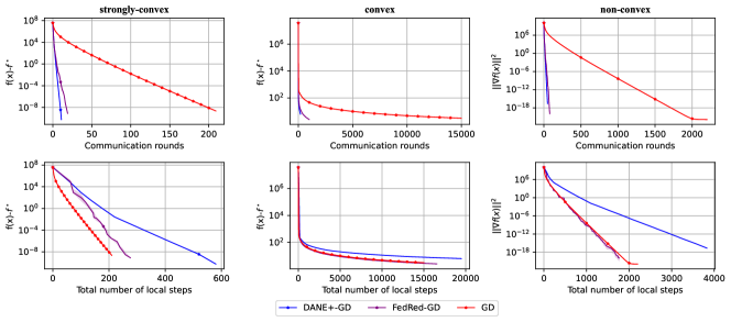
Figure 1: Illustrating communication reduction for DANE+-GD and FedRed-GD on synthetic dataset using quadratic loss with $\frac{L}{\delta_{A}}\approx\frac{L}{\delta_{B}}\gtrsim 20$. DANE+-GD and FedRed-GD require roughly $20$ times fewer communication rounds to reach the same suboptimality as GD while the total number of local computations of FedRed-GD is at the same scale as GD. (Repeated 3 times for FedRed-GD. The solid lines and the shaded area represent the mean and the region between the minimum and the maximum values.)

Related work.

The seminal work DANE (Shamir et al., 2014) is the first distributed algorithm that shows communication reduction for minimizing quadratics when the number of clients is large. Follow-up works interpret DANE as a preconditioning method. They provide better analysis and derive faster rates for quadratic losses (Zhang and Lin, 2015; Yuan and Li, 2019; Wang et al., 2018). Hendrikx et al. (2020) propose SPAG, an accelerated method, and prove a better uniform concentration bound of the conditioning number when solving strongly-convex problems. All these methods assume the iteration-subproblems can be solved exactly. (In this work, we study inexact local solvers for DANE).

On the other hand, federated optimization algorithms lean towards solving the subproblems inexactly by taking local updates. The standard FL method FedAvg has been shown ineffectiveness for convex optimization in the heterogeneous setting  (Woodworth et al., 2020). The celebrated Scaffold (Karimireddy et al., 2020) adds control variate to cope with the client drift issues in heterogeneous networks. It is also the first work to quantify the usefulness of local-steps for quadratics. Afterwards, drift correction is employed in many other works such as FedDC (Gao et al., 2022) and Adabest (Varno et al., 2022). FedPVR (Li et al., 2023) propose to apply drift correction only to the last layers of neural networks. Scaffnew (Mishchenko et al., 2022) first illustrates the usefulness of taking standard local gradient steps under strongy-convexity by using a special choice of control variate. More advanced methods with refined analysis and features such as client sampling and compression have been proposed (Hu and Huang, 2023; Condat et al., 2023; Grudzień et al., 2023; Condat and Richtárik, 2022). FedProx (Li et al., 2020) adds a proximal regularization term to the local functions to control the deviation between client and server models. FedDyn (Acar et al., 2021) proposes dynamic regularization to improve the convergence of FedProx. FedPD (Zhang et al., 2021) applies both drift correction and regularization and design the algorithm from the primal-dual perspective.

A more closely related line of research focuses on the study of convergence guarantee under relaxed function similarity conditions. SONATA (Sun et al., 2022) and Accelerated SONATA (Tian et al., 2022) provide better communication guarantee than vanilla GD under strong convexity. Accelerated ExtraGradient sliding improves the rate of (Tian et al., 2022) and allows the use of inexact local solvers. Khaled and Jin (2023) work with a more relaxed similarity assumption and propose a centralized stochastic proximal point variance-reduced method called SVRP. Mime combines drift correction with momentum for solving non-convex problems. Recently, CE-LGD (Patel et al., 2022) proposed to use recursive gradients together with momentum for non-convex distributed optimization.

2 Problem formulation and background

In this work, we consider the following distributed optimization problem:

$$\min_{\mathbf{x}\in\mathbb{R}^{d}}\biggl{[}f(\mathbf{x})=\frac{1}{n}\sum_{i=1}^{n}f_{i}(\mathbf{x})\biggr{]}\;.$$

We focus on the standard federated learning setting where $n$ clients jointly train a model and a central server coordinates the global learning procedure. Specifically, during each communication round $r=0,1,2...$,

1. the server broadcasts $\mathbf{x}^{r}$ to the clients;

2. each client $i\in[n]$ calls a local solver to compute the next iterate $\mathbf{x}_{i,r+1}$;

3. the server aggregates $\mathbf{x}^{r+1}$ using $(\mathbf{x}_{i,r+1})_{i=1}^{n}$.

Goal: We assume that establishing the connection between the server and the clients is expensive. Therefore, the main goal is to reduce the total number of communication rounds required to reach a desired accuracy.

Notations: We use $\mathbf{x}_{i}^{\star}$ and $\mathbf{x}^{\star}$ to denote $\operatorname*{arg\,min}_{x}\{f_{i}(\mathbf{x})\}$ and $\operatorname*{arg\,min}_{x}\{f(\mathbf{x})\}$ if they exist. We assume $f$ is lower bounded and denote the infimum of $f$ by $f^{\star}$.

Vanilla/Centralized GD. Gradient descent is a standard method that solves the problem. At each communication round $r$, each device computes its gradient $\nabla f_{i}(\mathbf{x}^{r})$, and performs one local gradient descent step: $\mathbf{x}_{i,r+1}=\mathbf{x}^{r}-\eta\nabla f_{i}(\mathbf{x}^{r})$. Then the server updates the global model by: $\mathbf{x}^{r+1}=\frac{1}{n}\sum_{i=1}^{n}\mathbf{x}_{i,r+1}$. The update rule can thus be written as: $\mathbf{x}^{r+1}=\mathbf{x}^{r}-\eta\nabla f(\mathbf{x}^{r})$. The convergence of this method is well understood (Nesterov, 2018).

Client drift. FedAvg or Local-(S)GD approximate the global function $f$ by $f_{i}$ on each device. Each device $i$ runs multiple (stochastic) gradient descent steps initialized at $\mathbf{x}^{r}$, i.e. $\mathbf{x}_{i,r+1}\approx\operatorname*{arg\,min}_{x}f_{i}(\mathbf{x})$. Then $\mathbf{x}^{r+1}={\frac{1}{n}\sum_{i=1}^{n}}\mathbf{x}_{i,r+1}$ is aggregated by the server.

This method suffers from client drift when $\{f_{i}\}$ are heterogeneous (Karimireddy et al., 2020; Khaled et al., 2019) because the local updates move towards the minimizers of each $f_{i}$. However, in general, ${\frac{1}{n}\sum_{i=1}^{n}}\mathbf{x}_{i}^{\star}\neq\mathbf{x}^{\star}$.

Regularization. To address the issue of client drift, FedProx (Li et al., 2020) proposes to add regularization to each local function $f_{i}$ to control the local iterates from deviating from the current global state, i.e. $\mathbf{x}_{i,r+1}\approx\operatorname*{arg\,min}_{x}\{f_{i}(\mathbf{x})+\frac{\lambda}{2}||\mathbf{x}-\mathbf{x}^{r}||^{2}\}$. However, the non-convergence issue still exists. Suppose we initialize at $\mathbf{x}^{\star}$ ($\mathbf{x}^{0}=\mathbf{x}^{\star}$), and local solvers return the exact minimizers. We have $\nabla f_{i}(\mathbf{x}_{i,1})+\lambda(\mathbf{x}_{i,1}-\mathbf{x}^{\star})=0$, which implies that $\mathbf{x}^{1}=\mathbf{x}^{\star}-\frac{1}{\lambda}{\frac{1}{n}\sum_{i=1}^{n}}\nabla f_{i}(\mathbf{x}_{i,1})$. Since $\mathbf{x}^{1}$ is typically not equal to $\mathbf{x}^{\star}$, $\mathbf{x}^{\star}$ is not a stationary point for FedProx.

Drift correction. Scaffold (Karimireddy et al., 2020) addresses the non-convergence issues by using drift correction. It approximates the global function by shifting each $f_{i}$ based on the current difference of gradients, i.e. $\mathbf{x}_{i,r+1}\approx\operatorname*{arg\,min}_{x}\{f_{i}(\mathbf{x})+\left\langle\nabla f(\mathbf{x}^{r})-\nabla f_{i}(\mathbf{x}^{r}),\mathbf{x}\right\rangle\}$, and uses (S)GD to solve the subproblem. However, Scaffold requires much smaller stepsize than GD to ensure convergence. Consequently, the overall communication complexity is no better than GD. Moreover, the subproblem itself is not well-defined. For instance, if some $f_{i}$ is a linear function, then the subproblem has no solution. Indeed, Scaffold can be viewed as a composite gradient descent method with stepsize set to be infinity, which we state as below.

Regularized drift correction. The appropriate solution to the previously mentioned issues is to incorporate both drift correction and regularization, a strategy already applied in DANE. Here, we provide a more intuitive explanation and cast it as a composite optimization method. Note that $f$ can be written as $f=f_{i}+\psi$ where $\psi:=f-f_{i}$. As each client has no access to $\psi$, the standard approach is to linearize $\psi$ at $\mathbf{x}^{r}$ and perform the composite gradient method: $\mathbf{x}_{i,r+1}\approx\operatorname*{arg\,min}\{f_{i}(\mathbf{x})+\left\langle\nabla\psi(\mathbf{x}^{r}),\mathbf{x}-\mathbf{x}^{r}\right\rangle+\frac{\lambda}{2}||\mathbf{x}-\mathbf{x}^{r}||^{2}\}$, where $\lambda>0$ should approximately be set to $||\nabla\psi^{2}(\mathbf{x}^{r})||$. If $||\nabla\psi^{2}(\mathbf{x}^{r})||$ is much smaller than the smoothness parameter of $f$, or equivalently if $f_{i}$ and $f$ have similar Hessians, then this approach can provably converge faster than GD. This motivates us to study the following algorithms which incorporate regularized drift correction to distributed optimization settings.

3 DANE+ with regularized drift correction

In this section, we first describe a framework that generalizes DANE (Algorithm 1) for distributed optimization with regularized drift correction. We then discuss how it achieves communication reduction when the functions of clients exhibit certain second-order similarities.

1:  Input: $\lambda\geq 0$, $\mathbf{x}^{0}\in\mathbb{R}^{d}$

2:  for $r=0,1,2...$ do

3:     for each client $i\in[n]$ in parallel do

4:        Update $\mathbf{h}_{i,r}$

5:        Set $\mathbf{x}_{i,r+1}\approx\operatorname*{arg\,min}_{\mathbf{x}\in\mathbb{R}^{d}}\bigl{\{}F_{i,r}(\mathbf{x})\bigr{\}}$, where

6:        $F_{i,r}(\mathbf{x}):=f_{i}(\mathbf{x})-\langle\mathbf{x},\mathbf{h}_{i,r}\rangle+\frac{\lambda}{2}||\mathbf{x}-\mathbf{x}^{r}||^{2}\;.$

7:     end for

8:     Set $\mathbf{x}^{r+1}=\text{Average}(\mathbf{x}_{i,r+1})_{i=1}^{n}$,

9:     where $\text{Average}(\cdot)$ denotes an averaging strategy.

10:  end for

Algorithm 1 DANE+

1:  Input: $p\in[0,1]$, $\lambda,\eta\geq 0$, $\mathbf{x}^{0}\in\mathbb{R}^{d}$

2:  Set $\mathbf{x}_{i,0}=\tilde{\mathbf{x}}_{0}=\mathbf{x}^{0}$, $\forall i\in[n]$.

3:  for $k=0,1,2...$ do

4:     for each client $i\in[n]$ in parallel do

5:        Update $\mathbf{h}_{i,k}$

6:                                                   $\mathbf{x}_{i,k+1}=\operatorname*{arg\,min}_{\mathbf{x}\in\mathbb{R}^{d}}\bigl{\{}F_{i,k}(\mathbf{x})\bigr{\}}\;.$

7:        where

$$F_{i,k}(\mathbf{x}):=f_{i}(\mathbf{x})-\left\langle\mathbf{x},\mathbf{h}_{i,k}\right\rangle+\frac{\eta}{2}||\mathbf{x}-\mathbf{x}_{i,k}||^{2}+\frac{\lambda}{2}||\mathbf{x}-\tilde{\mathbf{x}}_{k}||^{2}\;.$$

8:        Sample $\theta_{k}\in\{0,1\}$ where $\text{Prob}(\theta_{k}=1)=p$

9:                                           $\tilde{\mathbf{x}}_{k+1}=\begin{cases}\text{Average}(\mathbf{x}_{i,k+1})_{i=1}^{n}&\text{if }\theta_{k}=1\\ \tilde{\mathbf{x}}_{k}&\text{otherwise}\end{cases}\;.$

10:     end for

11:  end for

Algorithm 2 FedRed: Federated optimization framework with doubly Regularized drift correction

1:  The same as Algorithm 2, except on line 6

$$F_{i,k}(\mathbf{x}):=f_{i}(\mathbf{x}_{i,k})+\left\langle\mathbf{g}_{i}(\mathbf{x}_{i,k}),\mathbf{x}-\mathbf{x}_{i,k}\right\rangle-\left\langle\mathbf{x},\mathbf{h}_{i,k}\right\rangle+\frac{\eta}{2}||\mathbf{x}-\mathbf{x}_{i,k}||^{2}+\frac{\lambda}{2}||\mathbf{x}-\tilde{\mathbf{x}}_{k}||^{2}\;,$$

where $\mathbf{g}_{i}(\mathbf{x},\xi_{i})$ is a stochastic estimator of $\nabla f_{i}(\mathbf{x})$ for any $\mathbf{x}\in\mathbb{R}^{d}$.

Algorithm 3 FedRed-(S)GD

Method. During each communication round $r$ of DANE+, each client $i$ is assigned a local objective function $F_{i,r}$ and returns an approximate solution for it by running a local solver. The function $F_{i,r}$ has three standard components: i) the individual loss function $f_{i}$, ii) an inner product term for drift correction, and iii) a regularizer that controls the deviation of the local iterates from the current global model. After that, the server applies an averaging strategy to aggregate all the iterates returned by the clients.

To run the algorithm, we need to choose a control variate $\mathbf{h}_{i,r}$ and an averaging method.

Karimireddy et al. (2020) proposed two choices of control variates for drift correction. In this work, we study the properties of the standard one which is defined as follows:

$$\mathbf{h}_{i,r}:=\nabla f_{i}(\mathbf{x}^{r})-\nabla f(\mathbf{x}^{r})\;.$$ (1)

Another choice of control variate is also used in Scaffnew. In this work, we focus on Hessian Dissimilarity and defer the studies of that one for DANE+ to Appendix B.3.

There exist various ways of averaging vectors. Let $(\mathbf{x}_{i})_{i=1}^{n}$ be a set of vectors where $\mathbf{x}_{i}\in\mathbb{R}^{d}$. The standard averaging is defined as follows.

$$\text{Avg}(\mathbf{x}_{i})_{i=1}^{n}:=\textstyle{\frac{1}{n}\sum_{i=1}^{n}}\mathbf{x}_{i}\;.$$

In this work, we also work on randomized averaging:

$$\text{Rand}(\mathbf{x}_{i})_{i=1}^{n}:=\mathbf{x}_{\hat{j}}\;.$$

where $\hat{j}$ denotes a random variable that follows a fixed probability distribution at each iteration.

Suppose that control variate (1) is used, each local solver provides the exact solution, and that standard averaging is applied, then DANE+ is equivalent to DANE.

Communication Reduction. As discussed in Section 2, regularized drift correction can reduce the communication given that the functions $\{f_{i}\}$ are similar. A reasonable measure is to look at the second-order Hessian dissimilarity (Karimireddy et al., 2021, 2020; Zindari et al., 2023), which is defined as follows:

Definition 1 (Bounded Hessian Dissimilarity (Karimireddy et al., 2020)).

Let $f_{i}:\mathbb{R}^{d}\to\mathbb{R}$ be continuously differentiable for any $i\in[n]$, then $\{f_{i}\}$ have $\delta_{B}$-BHD if for any $\mathbf{x},\mathbf{y}\in\mathbb{R}^{d}$ and any $i\in[n]$,

$$||\nabla h_{i}(\mathbf{x})-\nabla h_{i}(\mathbf{y})||\leq\delta_{B}\;.$$ (2)

where $h_{i}:=f_{i}-f$, and $f:=\frac{1}{n}\sum_{i=1}^{n}f_{i}$.

The standard Bounded Hessian Dissimilarity defined in (Karimireddy et al., 2020) assumes $||\nabla h_{i}^{2}(\mathbf{x})||\leq\delta_{B}$ for any $\mathbf{x}\in\mathbb{R}^{d}$, which implies Definition 1 and is thus slightly stronger. Here, we only need first-order differentiability.

We also work on a weaker Hessian Dissimilarity definition.

Definition 2 (Averaged Hessian Dissimilarity (Khaled and Jin, 2023)).

Let $f_{i}:\mathbb{R}^{d}\to\mathbb{R}$ be continuously differentiable for any $i\in[n]$, then $\{f_{i}\}$ have $\delta_{A}$-AHD if for any $\mathbf{x},\mathbf{y}\in\mathbb{R}^{d}$,

$$\frac{1}{n}\sum_{i=1}^{n}||\nabla h_{i}(\mathbf{x})-\nabla h_{i}(\mathbf{y})||^{2}\leq\delta_{A}^{2}||\mathbf{x}-\mathbf{y}||^{2}\;.$$ (3)

where $h_{i}:=f_{i}-f$ and $f:=\frac{1}{n}\sum_{i=1}^{n}f_{i}$.

Even if each $f_{i}$ is twice-continuously differentiable, Definition 2 is still weaker than assuming ${\frac{1}{n}\sum_{i=1}^{n}}||\nabla h_{i}^{2}(\mathbf{x})||\leq\delta_{A}^{2}$ for any $\mathbf{x}\in\mathbb{R}^{d}$. The details can be found in Remark 18.

Suppose each $f_{i}$ is $L$-smooth, then $\delta_{A}\leq 2L$ and $\delta_{B}\leq 2L$. If further assuming each $f_{i}$ is convex, then $\delta_{A}\leq L$ and $\delta_{B}\leq L$. In practice, we expect the clients to be similar and thus $\delta_{A}\ll L$ and $\delta_{B}\ll L$ (Karimireddy et al., 2021). In principle, if each $h_{i}$ is $\delta_{i}$-smooth, then $\delta_{A}=(\frac{1}{n}\sum_{i}\delta_{i}^{2})^{1/2}$ can potentially be much smaller (up to $\sqrt{n}$ times) than $\delta_{B}=\max_{i}\{\delta_{i}\}$.

3.1 Theory

We state the convergence rates of DANE+ in this section. All the proofs can be found in Appendix B.

Nonconvex. When the local functions $\{f_{i}\}$ are non-convex, it becomes difficult to obtain an approximate minimizer of $F_{i,r}$. Instead, it is more realistic to assume that each local solver can converge to an approximate stationary point. In this case, the standard averaging may be less effective than randomized averaging, especially when $\{f_{i}\}$ are similar. The intuition is as follows.

Suppose that $f_{i}=f$ for any $i\in[n]$ . Then $F_{i,r}(\mathbf{x})\equiv f(\mathbf{x})$ if we set $\lambda=0$. Assume that each local solver can compute an exact stationary point. Then it is more reasonable to update the global model by selecting an update $\mathbf{x}_{i,r+1}$ rather than the standardally averaging all the iterates, as the averaged stationary points can be even worse. That being said, the standard averaging can still be effective and more stable if each client uses the same local solver. We leave this possibility in the future work.

In the following, we show that it is sufficient to arbitrarily choose a model from $(\mathbf{x}_{i,r+1})_{i=1}^{n}$ to update the global model. For instance, $\mathbf{x}^{r+1}=\text{Rand}(\mathbf{x}_{i,r+1})_{i=1}^{n}$. In practice, this index set can be predetermined and during each round, only a single client is required to do local updates.

Theorem 1.

Consider Algorithm 1 with control variate (1). Let the global model be updated by choosing an arbitrary local model for each communication round. Let $f_{i}:\mathbb{R}^{d}\to\mathbb{R}$ be continuously differentiable for any $i\in[n]$. Assume that $\{f_{i}\}$ have $\delta_{B}$-BHD. Suppose that the solutions returned by local solvers satisfy $F_{i,r}(\mathbf{x}_{i,r+1})\leq F_{i,r}(\mathbf{x}^{r})$ and $||\nabla F_{i,r}(\mathbf{x}_{i,r+1})||\leq e_{r+1}$ with $e_{r+1}\geq 0$ for any $r\geq 0$ and any $i\in[n]$. Let $\lambda=a\delta_{B}$ with $a>1$ Then after $R$ communication rounds, we have:

$$||\nabla f(\bar{\mathbf{x}}^{R})||^{2}\leq\frac{4(a+1)^{2}}{(a-1)}\frac{\delta_{B}(f(\mathbf{x}^{0})-f^{\star})}{R}+2\frac{1}{R}\sum_{r=1}^{R}e_{r}^{2}\;.$$

where $\bar{\mathbf{x}}^{R}=\arg\min_{\mathbf{x}\in\{\mathbf{x}^{r}\}_{r=0}^{R}}\{||\nabla f(\mathbf{x})||\}$.

Theorem 1 gives a convergence guarantee of DANE+ for arbitrary functions (not necessarily with Lipschitz gradient) with any local solvers. The minimal squared gradient norm decreases at a rate of $\mathcal{O}(\frac{\delta_{B}(f(\mathbf{x}^{0})-f^{\star})}{R})$. To reach arbitrary accuracy $\varepsilon$, the average errors should be at most $\varepsilon$. We next establish the local computational complexity assuming that the gradient of each $f_{i}$ is Lipschitz.

Corollary 2.

Consider Algorithm 1 with control variate (1). Let the global model be updated by choosing an arbitrary local model for each communication round. Let $f_{i}:\mathbb{R}^{d}\to\mathbb{R}$ be continuously differentiable and $L$-smooth for any $i\in[n]$. Assume that $\{f_{i}\}$ have $\delta_{B}$-BHD. Suppose each local solver runs the standard gradient descent starting from $\mathbf{x}^{r}$ for $\Theta\Bigl{(}\frac{L}{\delta_{B}}R\Bigr{)}$ local steps, for any $r\geq 0$, and returns the point with the minimum gradient norm. Let $\lambda=2\delta_{B}$. After $R$ communication rounds, we have:

$$||\nabla f(\bar{\mathbf{x}}^{R})||^{2}\leq\frac{72\delta_{B}(f(\mathbf{x}^{0})-f^{\star})}{R}\;.$$

where $\bar{\mathbf{x}}^{R}=\arg\min_{\mathbf{x}\in\{\mathbf{x}^{r}\}_{r=0}^{R}}\{||\nabla f(\mathbf{x})||\}$.

The communication complexity of DANE+-GD is reduced by a factor of $\frac{L}{\delta_{B}}$ compared with GD. However, the total gradient computations to reach $\varepsilon$ accuracy is $R=\Theta\bigl{(}\frac{\delta_{B}(f(\mathbf{x}^{0})-f^{\star})}{\varepsilon}\bigr{)}$ times worse than GD.

Convex. In contrast to non-convex problems, convex optimization can benefit from the standard averaging. This allows us to obtain the following convergence guarantee depending on the Averaged Hessian Dissimilarity.

Theorem 3.

Consider Algorithm 1 with control variate (1) and the standard averaging. Let $f_{i}:\mathbb{R}^{d}\to\mathbb{R}$ be continuously differentiable and $\mu$-convex with $\mu\geq 0$ for any $i\in[n]$. Assume that $\{f_{i}\}$ have $\delta_{A}$-AHD. In general, suppose that the solutions returned by local solvers satisfy ${\frac{1}{n}\sum_{i=1}^{n}}||\nabla F_{i,r}(\mathbf{x}_{i,r+1})||^{2}\leq e_{r+1}^{2}$ for any $r\geq 0$ with $e_{r+1}\geq 0$. Let $\lambda\geq 2\delta_{A}$. After $R$ communication rounds, we have:

$$\begin{split}f(\bar{\mathbf{x}}^{R})&-f(\mathbf{x}^{\star})+\frac{\mu}{2}{\frac{1}{n}\sum_{i=1}^{n}}||\mathbf{x}_{i,R}-\mathbf{x}^{\star}||^{2}\leq\\ &\frac{\mu}{(1+\frac{\mu}{\lambda})^{R}-1}||\mathbf{x}^{0}-\mathbf{x}^{\star}||^{2}+\frac{2}{\mu+\lambda}\sum_{r=1}^{R}e_{r}^{2}\;.\end{split}$$

where $\bar{\mathbf{x}}^{R}:=\operatorname*{arg\,min}_{\mathbf{x}\in\{\mathbf{x}^{r}\}_{r=1}^{R}}f(\mathbf{x})$.

Theorem 3 provides the convergence guarantee for DANE+ when the local functions are convex (and not necessarily smooth). Each local solver can be chosen arbitrarily, provided that it can return a solution that satisfies a specific accuracy condition. The convergence rate is a continuous estimate both in $\mu$ and $\lambda$, since $\frac{\mu}{(1+\frac{\mu}{\lambda})^{R}-1}\leq\frac{\lambda}{R}$. To reach a certain accuracy $\varepsilon$, the errors should satisfy $\sum_{r=1}^{R}e_{r}^{2}\leq\frac{\varepsilon(\mu+\lambda)}{2}$. We next show that if the solutions returned by local solvers satisfy more specific conditions, then the additional error term $\sum_{r=1}^{R}e_{r}^{2}$ can be removed.

Theorem 4.

Under the same conditions as Theorem 3, suppose that the solutions returned by local solvers satisfy $\sum_{i=1}^{n}||\nabla F_{i,r}(\mathbf{x}_{i,r+1})||^{2}\leq e_{r}^{2}\sum_{i=1}^{n}||\mathbf{x}_{i,r+1}-\mathbf{x}^{r}||^{2}$ for any $r\geq 0$ and $e_{r}\geq 0$. Let $\lambda\geq 2\delta_{A}$ and let $\sum_{r=0}^{+\infty}e_{r}^{2}\leq\frac{\lambda(\mu+\lambda)}{8}$. After $R$ communication rounds:

$$f(\bar{\mathbf{x}}^{R}) -f(\mathbf{x}^{\star})+\frac{\mu}{2}{\frac{1}{n}\sum_{i=1}^{n}}||\mathbf{x}_{i,R}-\mathbf{x}^{\star}||^{2}\leq$$

$$\frac{\mu}{[(1+\frac{\mu}{\lambda})^{R}-1]}||\mathbf{x}^{0}-\mathbf{x}^{\star}||^{2}\leq\frac{\lambda}{R}||\mathbf{x}^{0}-\mathbf{x}^{\star}||^{2}\;.$$

where $\bar{\mathbf{x}}^{R}:=\operatorname*{arg\,min}_{\mathbf{x}\in\{\mathbf{x}^{r}\}_{r=1}^{R}}f(\mathbf{x})$.

In practice, it is sufficient to stop running the local solver on each device once the solutions satisfy $||\nabla F_{i,r}(\mathbf{x}_{i,r+1})||\leq e_{r}||\mathbf{x}_{i,r+1}-\mathbf{x}^{r}||$ with $e_{r}^{2}:=\frac{\lambda(\mu+\lambda)}{8(r+1)(r+2)}.$ As a direct corollary of Theorem 4, we can estimate the required number of local iterations for standard first-order methods assuming that each function $f_{i}$ is $L$-smooth.

Corollary 5.

Consider Algorithm 1 with control variate (1) and standard averaging. Let $f_{i}:\mathbb{R}^{d}\to\mathbb{R}$ be continuously differentiable, $\mu$-convex with $\mu\geq 0$, and $L$-smooth for any $i\in[n]$. Assume that $\{f_{i}\}$ have $\delta_{A}$-AHD with $L\geq\delta_{A}+\mu$. Suppose for any $r\geq 0$, each device uses the standard (fast) gradient descent initialized at $\mathbf{x}^{r}$ until $||\nabla F_{i,r}(\mathbf{x}_{i,r+1})||^{2}\leq\frac{\lambda(\mu+\lambda)}{8(r+1)(r+2)}||\mathbf{x}_{i,r+1}-\mathbf{x}^{r}||^{2}$ is satisfied. Let $\lambda=2\delta_{A}$. To have the same convergence guarantee as in Theorem 4, the total number of local steps $K_{r}$ required at each round $r$ is no more than:

DANE+-GD:

$$K_{r}\leq\Theta\Biggl{(}\frac{L}{\delta_{A}+\mu}\ln\biggl{(}\frac{L}{\delta_{A}+\mu}(r+1)\biggr{)}\Biggr{)}\;.$$

DANE+-FGD:

$$K_{r}\leq\Theta\Biggl{(}\sqrt{\frac{L}{\delta_{A}+\mu}}\ln\biggl{(}\frac{L}{\delta_{A}+\mu}(r+1)\biggr{)}\Biggr{)}\;.$$

The total computational complexity of DANE+-GD is equivalent to that of the centralized gradient descent method, up to a logarithmic factor that depends on $r$.

4 FedRed: an optimization framework with Doubly Regularized Drift Correction

While DANE+ can achieve communication speed-up, the local computations are inefficient. This is because, for every communication round, a difficult subproblem has to be approximately solved. In this section, we present a general framework that improves the overall computational efficiency while maintaining the communication reduction.

Key idea: Let us add an additional regularizer to improve the conditioning of the subproblem. FedRed 2 retains two sequences throughout the iteration: $\{\mathbf{x}_{i,k}\}$ denote the iterates stored on each device, and $\{\tilde{\mathbf{x}}_{k}\}$ are the reference points. At each iteration $k$, FedRed adds an additional regularizer to the proxy function defined in DANE+. By setting $\eta$ to be a large number (e.g. $2L$ where $L$ is the Lipschitz constant), $F_{i,k}$ can become a function with a good condition number (an absolute constant) and thus can be solved efficiently in a constant (up to the logarithmic factor) number of steps.

However, strong regularization prevents aggressive progress of the algorithm. Therefore, the communication is only triggered with probability $p$, with the reference points being adjusted to the averaged $(\mathbf{x}_{i,k+1})_{i=1}^{n}$. Lastly, the control variates $\{\mathbf{h}_{i,k}\}$ are updated accordingly. We study the same control variate as defined in (1):

$$\mathbf{h}_{i,k}:=\nabla f_{i}(\tilde{\mathbf{x}}_{k})-\nabla f(\tilde{\mathbf{x}}_{k})\;.$$ (4)

Note that DANE+ becomes a special case of FedRed when $p=1$ and $\eta=0$. We next show the convergence rates for FedRed using exact local solvers.

4.1 FedRed with Exact Solvers

Theorem 6.

Consider Algorithm 2 with control variate (4) and randomized averaging with random index set $\{i_{k}\}_{k=0}^{+\infty}$. Let $f_{i}:\mathbb{R}^{d}\to\mathbb{R}$ be continuously differentiable for any $i\in[n]$. Assume that $\{f_{i}\}$ have $\delta_{B}$-BHD. Let $\lambda=\delta_{B}$, $p=\frac{\lambda}{\eta}$ and $\eta\geq 4\delta_{B}$. For any $K\geq 1$, it holds that:

$$\operatorname{{\mathbb{E}}}\Bigl{[}||\nabla f(\bar{\mathbf{x}}_{K})||^{2}\Bigr{]}\leq\frac{150\eta(f(\mathbf{x}^{0})-f^{\star})}{K}\;,$$

where $\bar{\mathbf{x}}_{K}$ is uniformly sampled from $(\mathbf{x}_{i_{k},k})_{k=0}^{K-1}$.

To reach $\varepsilon$-accuracy, the communication complexity is $p\mathcal{O}(\frac{\eta}{K})=\mathcal{O}(\frac{\delta_{B}}{\varepsilon})$ in expectation, which is the same as DANE+. However, due to the additional regularization, the subproblem becomes easier to solve. The same conclusion can also be derived for the convex settings.

Theorem 7.

Consider Algorithm 2 with control variate (4) and the standard averaging. Let $f_{i}:\mathbb{R}^{d}\to\mathbb{R}$ be continuously differentiable, $\mu$-convex with $\mu\geq 0$ for any $i\in[n]$. Assume that $\{f_{i}\}$ have $\delta_{A}$-AHD. By choosing $p=\frac{\lambda+\mu/2}{\eta+\mu/2}$ and $\eta\geq\lambda\geq\delta_{A}$, for any $K\geq 1$, it holds that:

$$\begin{split}&\operatorname{{\mathbb{E}}}[f(\bar{\bar{\mathbf{x}}}_{K})-f^{\star}]+\frac{\mu}{4}\operatorname{{\mathbb{E}}}\biggl{[}||\tilde{\mathbf{x}}_{K}-\mathbf{x}^{\star}||^{2}+\frac{1}{n}\sum_{i=1}^{n}||\mathbf{x}_{i,K}\\ &-\mathbf{x}^{\star}||^{2}\biggr{]}\leq\frac{\mu}{2}\frac{||\mathbf{x}_{0}-\mathbf{x}^{\star}||^{2}}{(1+\frac{\mu}{2\eta})^{K}-1}\leq\frac{\eta||\mathbf{x}_{0}-\mathbf{x}^{\star}||^{2}}{K}\;.\end{split}$$

where $\bar{\bar{\mathbf{x}}}_{K}:=\sum_{k=1}^{K}\frac{1}{q^{k}}\bar{\mathbf{x}}_{k}/\sum_{k=1}^{K}\frac{1}{q^{k}}$, $\bar{\mathbf{x}}_{k}:={\frac{1}{n}\sum_{i=1}^{n}}\mathbf{x}_{i,k}$, and $q:=1-\frac{\mu}{2\eta+\mu}$.

4.2 Comparison to existing algorithms.

In this section, we compare FedRed with two similar algorithms. SVRP (Khaled and Jin, 2023) is a stochastic proximal point variance-reduced method. As discussed in the introduction, the main focus of SVRP is different in this paper. The main algorithmic differences between SVRP and FedRed are that: 1) FedRed uses double regularization and thus the regularized centering points are different 2) For SVRP, communication happens at each iteration , while FedRed skips communication with probability $1-p$, and 3) FedRed allows standard averaging for convex optimization. Another similar algorithm is FedPD (Zhang et al., 2021) where regularized drift correction and the strategy of skipping communication with probability are used. However, due to the different regularizations, FedPD is less efficient in local computations.

4.3 FedRed-(S)GD

Previous theorems assume that the exact minimizers (or stationary points) of the subproblems are returned at each iteration. In this section, we show that, in fact, it suffices to make only one local step for minimizing smooth functions.

Note the derivation of Algorithm 3 is to simply linearize $f_{i}$ at $\mathbf{x}_{i,k}$. Therefore, the solution of the subproblem has a closed form: $\mathbf{x}_{i,k+1}=\frac{\eta}{\eta+\lambda}\mathbf{x}_{i,k}+\frac{\lambda}{\eta+\lambda}\tilde{\mathbf{x}}_{k}-\frac{1}{\eta+\lambda}(\mathbf{g}_{i}(\mathbf{x}_{i,k})-\mathbf{h}_{i,k})$, which is a convex combination of $\mathbf{x}_{i,k}$ and $\tilde{\mathbf{x}}_{k}$ followed by a gradient descent step.

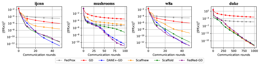
Figure 2: Comparison of DANE+-GD and FedRed-GD against four other distributed optimizers on four LIBSVM datasets using regularized logistic loss.

Here we allow the use of a stochastic gradient $\mathbf{g}_{i}(\mathbf{x},\xi_{i})$ instead of the full gradient $\nabla f_{i}(\mathbf{x})$. While more extensions could be made such as approximating $\mathbf{h}_{i,k}$ using stochastic gradients, we do not attempt to be exhaustive here as the goal is to illustrate the communication reduction. We make the following standard assumptions for $\mathbf{g}_{i}(\mathbf{x},\xi_{i})$.

Assumption 1.

For any $i\in[n]$, $\mathbf{g}_{i}(\mathbf{x},\xi_{i})$ is an unbiased stochastic estimator of $\nabla f_{i}(\mathbf{x})$ with bounded variance $\sigma^{2}$ such that for any $\mathbf{x}\in\mathbb{R}^{d}$, it holds that:

$$\operatorname{{\mathbb{E}}}[\mathbf{g}_{i}(\mathbf{x})]=\nabla f_{i}(\mathbf{x}),\quad\operatorname{{\mathbb{E}}}[||\mathbf{g}_{i}(\mathbf{x})-\nabla f_{i}(\mathbf{x})||^{2}]\leq\sigma^{2}.$$ (5)

Theorem 8.

Consider Algorithm 3 with control variate (4) and randomized averaging with random index set $\{i_{k}\}_{k=0}^{+\infty}$. Let $f_{i}:\mathbb{R}^{d}\to\mathbb{R}$ be continuously differentiable and $L$-smooth for any $i\in[n]$. Assume that $\{f_{i}\}$ have $\delta_{B}$-BHD with $\delta_{B}\leq L$ and that Assumption 1 holds. By choosing $\eta=3L+\sqrt{9L^{2}+\frac{L\sigma^{2}K}{f(\mathbf{x}^{0})-f^{\star}}}$, $\lambda=\delta_{B}$ and $p=\frac{\delta_{B}}{L}$, for any $K\geq 1$, it holds that:

$$\operatorname{{\mathbb{E}}}\bigl{[}||\nabla f(\bar{\mathbf{x}}_{K})||^{2}\bigr{]} \leq\frac{96L(f(\mathbf{x}^{0})-f^{\star})}{K}$$ (6)

$$+24\sqrt{\frac{L(f(\mathbf{x}^{0})-f^{\star})}{K}}\sigma\;.$$ (7)

where $\bar{\mathbf{x}}_{K}$ is uniformly sampled from $(\mathbf{x}_{i_{k},k})_{k=0}^{K-1}$.

According to Theorem 8, FedRed-GD (using full-batch gradient) requires the same total gradient computations as gradient descent to reach a certain accuracy. However, in expectation, it can skip communication for every $\Theta(\frac{L}{\delta_{B}})$ steps without additional cost.

Theorem 9.

Consider Algorithm 3 with control variate (4) and the standard averaging. Let $f_{i}:\mathbb{R}^{d}\to\mathbb{R}$ be continuously differentiable, $\mu$-convex with $\mu\geq 0$ and $L$-smooth for any $i\in[n]$. Assume that $\{f_{i}\}$ have $\delta_{A}$-AHD with $\delta_{A}+\mu\leq L$ and that Assumption 1 holds. Let $\lambda=\delta_{A}$, $p=\frac{\lambda+\mu/2}{\eta-\mu/2}$, and $\eta>L$. To reach $\varepsilon$-accuracy, i.e. $\operatorname{{\mathbb{E}}}[f(\bar{\bar{\mathbf{x}}}_{K})-f^{\star}]\leq\varepsilon$, by choosing $\eta=\frac{\sigma^{2}}{\varepsilon}+L$, the total number of iterations is no more than:

$$K\leq\Biggl{\lceil}\Bigl{(}\frac{2L}{\mu}+\frac{2\sigma^{2}}{\mu\varepsilon}\Bigr{)}\ln\Bigl{(}1+\frac{\mu||\mathbf{x}^{0}-\mathbf{x}^{\star}||^{2}}{\varepsilon}\Bigr{)}\Biggr{\rceil}\;.$$

where $\bar{\bar{\mathbf{x}}}_{K}:=\sum_{k=1}^{K}\frac{1}{q^{k}}\bar{\mathbf{x}}_{k}/\sum_{k=1}^{K}\frac{1}{q^{k}}$, $\bar{\mathbf{x}}_{k}:={\frac{1}{n}\sum_{i=1}^{n}}\mathbf{x}_{i,k}$, and $q:=1-\frac{\mu}{2\eta-\mu}$.

Since $\Bigl{(}\frac{2L}{\mu}+\frac{2\sigma^{2}}{\mu\varepsilon}\Bigr{)}\ln\Bigl{(}1+\frac{\mu||\mathbf{x}^{0}-\mathbf{x}^{\star}||^{2}}{\varepsilon}\Bigr{)}\leq\frac{2L||\mathbf{x}^{0}-\mathbf{x}^{\star}||^{2}}{\varepsilon}+\frac{2\sigma^{2}||\mathbf{x}^{0}-\mathbf{x}^{\star}||^{2}}{\varepsilon^{2}}$, the estimate of $K$ is continuous in $\mu$. Let us suppose $\sigma=0$ and $\mu=0$ for simplicity. FedRed-GD achieves the same computational complexity $K=\mathcal{O}(\frac{L}{\varepsilon})$ as GD. However, the communication complexity is $pK=\mathcal{O}(\frac{\delta_{A}}{\varepsilon})$ which is $\frac{L}{\delta_{A}}$ times faster than GD. The same conclusion remains effective where $\mu>0$.

Discussion. Corollary 5 shows DANE+-FGD achieves a faster local convergence rate than DANE+-GD. We suspect the fast gradient method can also improve complexity for FedRed. We leave this potential as a future work.

5 Experiments

In this section, we illustrate the main theoretical properties of our studied methods in numerical experiments on both simulated and real datasets.

Synthetic data. We consider the minimization problem of the form: $f(\mathbf{x})={\frac{1}{n}\sum_{i=1}^{n}}f_{i}(\mathbf{x})$ where $f_{i}(\mathbf{x}):=\frac{1}{m}\sum_{j=1}^{m}\frac{1}{2}(\mathbf{x}-\mathbf{b}_{i,j})^{T}A_{i,j}(\mathbf{x}-\mathbf{b}_{i,j})+\beta\sum_{k=1}^{d}\frac{[\mathbf{x}]_{k}^{2}}{1+[\mathbf{x}]_{k}^{2}}$, $\mathbf{b}_{i,j}\in\mathbb{R}^{d}$, $A_{i,j}\in\mathbb{R}^{d\times d}$, and $[\cdot]_{k}$ is an indexing operation of a vector. We set $\beta=0$ for convex problems and $\beta=400$ for the non-convex case. We further use $n=5$, $m=10$, and $d=1000$. Note that $\delta_{A}=\sqrt{{\frac{1}{n}\sum_{i=1}^{n}}||\bar{A}_{i}-\bar{A}||^{2}}$ and $\delta_{B}=\max_{i}\{||\bar{A}_{i}-\bar{A}||\}$ where $\bar{A}_{i}:=\frac{1}{m}\sum_{j=1}^{m}A_{i,j}$, and $\bar{A}:={\frac{1}{n}\sum_{i=1}^{n}}\bar{A}_{i}$. We generate $\{A_{i,j}\}$ such that $\max_{i,j}\{||A_{i,j}||\}=100$ and $\delta_{A}\approx\delta_{B}\approx 5$. We generate a strongly-convex instance by further controlling the minimum eigenvalue of $A_{i,j}$ to be $1$, and a general convex instance by setting some of the eigenvalues to small values close to zero (while ensuring that each $A_{i,j}$ is positive semi-definite). For the non-convex instance, we leave each $A_{i,j}$ as an indefinite matrix. By these constructions, we have that $\frac{L}{\delta_{A}}\approx\frac{L}{\delta_{B}}\gtrsim 20$.

We compare DANE+-GD and FedRed-GD against the vanilla gradient descent method. We compute approximate solutions for DANE+-GD by running local gradient descent until certain stopping criteria are reached. We use the constant probability ($\approx 0.05$) schedule for FedRed-GD. Lastly, we set the same step size for all three methods. In Figure 1, we can observe that both DANE+-GD and FedRed-GD require approximately $20$ times fewer communication rounds than GD to reach the same accuracy. More importantly, the total cost of gradient computation for FedRed-GD is at the same scale as GD, demonstrating the usefulness of local steps and validating the theory.

Binary classification on LIBSVM datasets. We experiment with the binary classification task on four real-world LIBSVM datasets (Chang and Lin, 2011). We use the standard regularized logistic loss: $f(\mathbf{x})={\frac{1}{n}\sum_{i=1}^{n}}f_{i}(\mathbf{x})$ with $f_{i}(\mathbf{x}):=\frac{n}{M}\sum_{j=1}^{m_{i}}\log(1+\exp(-y_{i,j}\mathbf{a}_{i,j}^{T}\mathbf{x}))+\frac{1}{2M}||\mathbf{x}||^{2}$ where $(\mathbf{a}_{i,j},y_{i,j})\in\mathbb{R}^{d+1}$ are feature and labels and $M:=\sum_{i=1}^{n}{m_{i}}$ is the total number of data points in the training dataset. We use $n=5$ and split the dataset according to the Dirichlet distribution. We benchmark against popular distributed algorithms including Scaffold (Karimireddy et al., 2020), Scaffnew (Mishchenko et al., 2022), Fedprox (Li et al., 2020), and GD. We use control variate (4) for Scaffold. We perform grid search to find the best hyper-parameters for each algorithm including the number of local steps and the stepsizes. From Figure 2, we observe that DANE+-GD and FedRed-GD consistently achieve fast convergence due to the implicit similarities of the objective functions among the workers.

Deep learning tasks. We defer the study of our proposed algorithms for image classification tasks using ResNet-18 (He et al., 2016) to Appendix C. More experiments with different neural network structures on various datasets need to be further investigated.

Practical choices of hyper-parameters. For FedRed, the main theories suggest that $p\sim\frac{\delta_{A}}{L}$ for convex problems and $p\sim\frac{\delta_{B}}{L}$ for non-convex instances. The stepsize $\eta$ should be of order $L$. Hence, we can always fix $\lambda=p\eta$ which has the same order as the similarity constant.

6 Conclusion

We propose a new federated optimization framework that simultaneously achieves both communication reduction and efficient local computations. Interesting future directions may include: theoretical analysis for client sampling and inexact control variates, extensions to the decentralized settings, accelerated version of FedRed, a more comprehensive study of FedRed and DANE+ for deep learning.

Appendix

Appendix A Technical Preliminaries

A.1 Basic Definitions

We use the following definitions throughout the paper.

Definition 3 (Convexity).

A differentiable function $f:\mathbb{R}^{d}\to\mathbb{R}$ is $\mu$-convex with $\mu\geq 0$ if $\forall\;\mathbf{x},\mathbf{y}\in\mathbb{R}^{d}$,

$$f(\mathbf{y})\geq f(\mathbf{x})+\left\langle\nabla f(\mathbf{x}),\mathbf{y}-\mathbf{x}\right\rangle+\frac{\mu}{2}||\mathbf{x}-\mathbf{y}||^{2}\;.$$ (A.1)

Definition 4 ($L$-smooth).

Let function $f:\mathbb{R}^{d}\to\mathbb{R}$ be differentiable. $f$ is smooth if there exists $L\geq 0$ such that $\forall\;\mathbf{x},\mathbf{y}\in\mathbb{R}^{d}$,

$$||\nabla f(\mathbf{x})-\nabla f(\mathbf{y})||\leq L||\mathbf{x}-\mathbf{y}||\;.$$ (A.2)

A.2 Useful Lemmas

We frequently use the following helpful lemmas for the proofs.

Lemma 10.

Let $\mathbf{x},\mathbf{y}\in\mathbb{R}^{d}$. For any $\gamma>0$, we have:

$$-\frac{1}{2\gamma}||\mathbf{x}||^{2}-\frac{\gamma}{2}||\mathbf{y}||^{2}\leq\left\langle\mathbf{x},\mathbf{y}\right\rangle\leq\frac{1}{2\gamma}||\mathbf{x}||^{2}+\frac{\gamma}{2}||\mathbf{y}||^{2}\;,$$ (A.3)

$$||\mathbf{x}+\mathbf{y}||^{2}\leq(1+\gamma)||\mathbf{x}||^{2}+\Bigl{(}1+\frac{1}{\gamma}\Bigr{)}||\mathbf{y}||^{2}\;.$$ (A.4)

Lemma 11.

Let $\mathbf{x}\in\mathbb{R}^{d}$ and $a>0$. For any $\mathbf{y}\in\mathbb{R}^{d}$, we have:

$$\left\langle\mathbf{x},\mathbf{y}\right\rangle+\frac{a}{2}||\mathbf{y}||^{2}\geq-\frac{||\mathbf{x}||^{2}}{2a}\;.$$ (A.5)

Proof.

The claim follows from the first-order optimality condition. ∎

Lemma 12.

Let $\{x_{r}\}_{r=0}^{+\infty}$ be a non-negative sequence such that $x_{r+1}-x_{r}\leq a_{r+1}\sqrt{x_{r+1}}$ for any $r\geq 0$, where $a_{i}\geq 0$ for any $i\geq 1$. Then for any $R\geq 1$, we have:

$$x_{R}\leq\Bigl{(}\sqrt{x_{0}}+\sum_{r=1}^{R}a_{r}\Bigr{)}^{2}\leq 2x_{0}+2\Bigl{(}\sum_{r=1}^{R}a_{r}\Bigr{)}^{2}\;.$$ (A.6)

Proof.

Indeed, for any $r\geq 0$, we have:

$$x_{r+1}-x_{r}=(\sqrt{x_{r+1}}-\sqrt{x_{r}})(\sqrt{x_{r+1}}+\sqrt{x_{r}})\geq(\sqrt{x_{r+1}}-\sqrt{x_{r}})\sqrt{x_{r+1}}\;.$$ (A.7)

It follows that:

$$\sqrt{x_{r+1}}\leq\sqrt{x_{r}}+a_{r+1}\;.$$ (A.8)

Summing up from $r=0$ to $R-1$, we get:

$$\sqrt{x_{R}}\leq\sqrt{x_{0}}+\sum_{r=1}^{R}a_{r}\;.$$ (A.9)

Taking the square on both sides, we have:

$$x_{R}\leq\Bigl{(}\sqrt{x_{0}}+\sum_{r=1}^{R}a_{r}\Bigr{)}^{2}\leq 2x_{0}+2\Bigl{(}\sum_{r=1}^{R}a_{r}\Bigr{)}^{2}\;.\qed$$ (A.10)

Lemma 13.

Let $q>0$ and let $(F_{k})_{k=1}^{+\infty}$, $(D_{k})_{k=1}^{+\infty}$ be two non-negative sequences such that: $F_{k+1}+D_{k+1}\leq qD_{k}$ for any $k\geq 0$. Then for any $K\geq 1$, it holds that:

$$\frac{1}{S_{k}}\sum_{k=1}^{K}\frac{F_{k}}{q^{k}}+\frac{1-q}{1-q^{K}}D_{K}\leq\frac{1-q}{\frac{1}{q^{K}}-1}D_{0}\;,$$ (A.11)

where $S_{k}:=\sum_{k=1}^{K}\frac{1}{q^{k}}$.

Proof.

Indeed, for any $k\geq 0$, we have:

$$\frac{F_{k+1}}{q^{k+1}}+\frac{D_{k+1}}{q^{k+1}}\leq\frac{D_{k}}{q^{k}}\;.$$ (A.12)

Summing up from $k=0$ to $K-1$, we get:

$$\sum_{k=1}^{K}\frac{F_{k}}{q^{k}}+\frac{D_{K}}{q^{K}}\leq D_{0}\;.$$ (A.13)

Dividing both sides by $\sum_{k=1}^{K}\frac{1}{q^{k}}$ and using the fact that $\sum_{k=1}^{K}\frac{1}{q^{k}}=\frac{\frac{1}{q^{K}}-1}{1-q}$, we obtain:

$$\frac{1-q}{\frac{1}{q^{K}}-1}\sum_{k=1}^{K}\frac{F_{k}}{q^{k}}+\frac{1-q}{1-q^{K}}D_{K}\leq\frac{1-q}{\frac{1}{q^{K}}-1}D_{0}\;.$$ (A.14)

∎

Lemma 14.

Let $\{x_{i}\}_{i=1}^{n}$ be a set of vectors in $\mathbb{R}^{d}$ and let $\mathbf{v}\in\mathbb{R}^{d}$ be an arbitrary vector. It holds that:

$${\frac{1}{n}\sum_{i=1}^{n}}||\mathbf{x}_{i}-\mathbf{v}||^{2}\ =||\mathbf{x}-\mathbf{v}||^{2}+{\frac{1}{n}\sum_{i=1}^{n}}||\mathbf{x}_{i}-\mathbf{x}||^{2},\quad\text{with}\quad\mathbf{x}:={\frac{1}{n}\sum_{i=1}^{n}}\mathbf{x}_{i}\;.$$ (A.15)

Proof.

Indeed,

$${\frac{1}{n}\sum_{i=1}^{n}}||\mathbf{x}_{i}-\mathbf{v}||^{2} ={\frac{1}{n}\sum_{i=1}^{n}}||\mathbf{x}_{i}-\mathbf{x}+\mathbf{x}-\mathbf{v}||^{2}$$ (A.16)

$$={\frac{1}{n}\sum_{i=1}^{n}}\Bigl{[}||\mathbf{x}_{i}-\mathbf{x}||^{2}+2\left\langle\mathbf{x}_{i}-\mathbf{x},\mathbf{x}-\mathbf{v}\right\rangle+||\mathbf{x}-\mathbf{v}||^{2}\Bigr{]}$$ (A.17)

$$=||\mathbf{x}-\mathbf{v}||^{2}+{\frac{1}{n}\sum_{i=1}^{n}}||\mathbf{x}_{i}-\mathbf{x}||^{2}\;.\qed$$ (A.18)

Lemma 15 (Nesterov (2018), Lemma 1.2.3).

Smoothness (A.2) implies that there exists a quadratic upper bound on f:

$$f(\mathbf{y})\leq f(\mathbf{x})+\left\langle\nabla f(\mathbf{x}),\mathbf{y}-\mathbf{x}\right\rangle|+\frac{L}{2}||\mathbf{y}-\mathbf{x}||^{2},\;\forall\mathbf{x},\mathbf{y}\in\mathbb{R}^{d}\;.$$ (A.19)

Lemma 16 (Nesterov (2018), Theorem 2.1.12).

Suppose a function $f$ is $L$-smooth and $\mu$-convex, then it holds that:

$$\left\langle\nabla f(\mathbf{x})-\nabla f(\mathbf{y}),\mathbf{x}-\mathbf{y}\right\rangle\geq\frac{\mu L}{\mu+L}||\mathbf{x}-\mathbf{y}||^{2}+\frac{1}{\mu+L}||\nabla f(\mathbf{x})-\nabla f(\mathbf{y})||^{2},\qquad\forall\mathbf{x},\mathbf{y}\in\mathbb{R}^{d}.$$ (A.20)

Lemma 17 (Hessian Dissimilarity).

Let $h_{i}:\mathbb{R}^{d}\to\mathbb{R}$ be twice continuously differentiable for any $i\in[n]$. Suppose for any $\mathbf{x}\in\mathbb{R}^{d}$ and any $p\geq 1$, it holds that:

$$\frac{1}{n}\sum_{i=1}^{n}||\nabla^{2}h_{i}(\mathbf{x})||^{p}\leq\delta^{p}\;.$$ (A.21)

Then for any $\mathbf{x},\mathbf{y}\in\mathbb{R}^{d}$, we have:

$$\frac{1}{n}\sum_{i=1}^{n}||\nabla h_{i}(\mathbf{x})-\nabla h_{i}(\mathbf{y})||^{p}\leq\delta^{p}||\mathbf{x}-\mathbf{y}||^{p}\;.$$ (A.22)

Proof.

Since $h_{i}$ is twice continuously differentiable, by Taylor’s Theorem, we have:

$$\nabla h_{i}(\mathbf{y})=\nabla h_{i}(\mathbf{x})+\int_{0}^{1}\nabla^{2}h_{i}(\mathbf{x}+t(\mathbf{y}-\mathbf{x}))[\mathbf{y}-\mathbf{x}]dt\;.$$ (A.23)

It follows that:

$$||\nabla h_{i}(\mathbf{y})-\nabla h_{i}(\mathbf{x})||^{p} =\Bigl{|}\Bigl{|}\int_{0}^{1}\nabla^{2}h_{i}(\mathbf{x}+t(\mathbf{y}-\mathbf{x}))[\mathbf{y}-\mathbf{x}]dt\Bigl{|}\Bigl{|}^{p}$$ (A.24)

$$\leq\biggl{[}\int_{0}^{1}||\nabla^{2}h_{i}(\mathbf{x}+t(\mathbf{y}-\mathbf{x}))||||\mathbf{y}-\mathbf{x}||dt\biggr{]}^{p}$$ (A.25)

$$=||\mathbf{y}-\mathbf{x}||^{p}\biggl{[}\int_{0}^{1}||\nabla^{2}h_{i}(\mathbf{x}+t(\mathbf{y}-\mathbf{x}))||dt\biggr{]}^{p}$$ (A.26)

$$\leq||\mathbf{y}-\mathbf{x}||^{p}\int_{0}^{1}||\nabla^{2}h_{i}(\mathbf{x}+t(\mathbf{y}-\mathbf{x}))||^{p}dt\;.$$ (A.27)

where in the last inequality, we use the Jensen’s inequality and the fact that $\tau\mapsto\tau^{p}$ is a convex function for $p\geq 1$.

By our assumption that $\frac{1}{n}\sum_{i=1}^{n}||\nabla^{2}h_{i}(\mathbf{z})||^{p}\leq\delta^{p}$ for any $\mathbf{z}\in\mathbb{R}^{d}$, we get:

$${\frac{1}{n}\sum_{i=1}^{n}}||\nabla h_{i}(\mathbf{y})-\nabla h_{i}(\mathbf{x})||^{p} \leq||\mathbf{y}-\mathbf{x}||^{p}\int_{0}^{1}{\frac{1}{n}\sum_{i=1}^{n}}||\nabla^{2}h_{i}(\mathbf{x}+t(\mathbf{y}-\mathbf{x}))||^{p}dt$$ (A.28)

$$\leq\delta^{p}||\mathbf{y}-\mathbf{x}||^{p}\;.\qed$$ (A.29)

Remark 18.

According to Lemma 17, if each $f_{i}$ is twice continuously differentiable and satisfies: ${\frac{1}{n}\sum_{i=1}^{n}}||\nabla^{2}f_{i}(\mathbf{x})-\nabla f^{2}(\mathbf{x})||^{2}\leq\delta_{A}^{2}$, for any $\mathbf{x}\in\mathbb{R}^{d}$, then $\{f_{i}\}$ have $\delta_{A}$-AHD. However the reverse does not hold. Let $n=3$ and $h_{i}:=f_{i}-f:=\frac{1}{2}\mathbf{x}^{T}\mathbf{A}_{i}\mathbf{x}$, where $\mathbf{x}\in\mathbb{R}^{2}$ and

$$\mathbf{A}_{1}=\begin{pmatrix}3&0\\ 0&2\end{pmatrix}\quad\mathbf{A}_{2}=\begin{pmatrix}-1&0\\ 0&1\end{pmatrix}\quad\mathbf{A}_{3}=\begin{pmatrix}-2&0\\ 0&-3\end{pmatrix}\quad\;.$$ (A.30)

It holds that:

$${\frac{1}{n}\sum_{i=1}^{n}}||\nabla h_{i}(\mathbf{x})-\nabla h_{i}(\mathbf{y})||^{2}=\frac{9+1+4}{3}||\mathbf{x}-\mathbf{y}||^{2}=\frac{14}{3}||\mathbf{x}-\mathbf{y}||^{2}\;,\forall\mathbf{x},\mathbf{y}\in\mathbb{R}^{2}\;.$$ (A.31)

On the other hand,

$${\frac{1}{n}\sum_{i=1}^{n}}||\nabla^{2}h_{i}(\mathbf{x})||^{2}=\frac{9+1+9}{3}=\frac{19}{3},\quad\forall\mathbf{x}\in\mathbb{R}^{2}\;.$$ (A.32)

Appendix B Proofs of main results

B.1 Convex results and proofs for Algorithm 1 with control variate (1)

Lemma 19.

Consider Algorithm 1. Let $f_{i}:\mathbb{R}^{d}\to\mathbb{R}$ be $\mu$-convex with $\mu\geq 0$ for any $i\in[n]$. Then for any $r\geq 0$, and any $\mathbf{x}\in\mathbb{R}^{d}$, we have:

$$f_{i}(\mathbf{x})-\left\langle\mathbf{x},\mathbf{h}_{i,r}\right\rangle+\frac{\lambda}{2}||\mathbf{x}-\mathbf{x}^{r}||^{2}\geq f_{i}(\mathbf{x}_{i,r+1}) -\left\langle\mathbf{x}_{i,r+1},\mathbf{h}_{i,r}\right\rangle+\frac{\lambda}{2}||\mathbf{x}_{i,r+1}-\mathbf{x}^{r}||^{2}$$ (B.1)

$$+\left\langle\nabla F_{i,r}(\mathbf{x}_{i,r+1}),\mathbf{x}-\mathbf{x}_{i,r+1}\right\rangle+\frac{\mu+\lambda}{2}||\mathbf{x}_{i,r+1}-\mathbf{x}||^{2}\;.$$ (B.2)

Proof.

Let $F_{i,r}(\mathbf{x}):=f_{i}(\mathbf{x})-\left\langle\mathbf{x},\mathbf{h}_{i,r}\right\rangle+\frac{\lambda}{2}||\mathbf{x}-\mathbf{x}^{r}||^{2}$. Since $F_{i,r}$ is $(\mu+\lambda)$-convex, we have:

$$F_{i,r}(\mathbf{x}) \stackrel{{\scriptstyle\eqref{df:stconvex}}}{{\geq}}F_{i,r}(\mathbf{x}_{i,r+1})+\left\langle\nabla F_{i,r}(\mathbf{x}_{i,r+1}),\mathbf{x}-\mathbf{x}_{i,r+1}\right\rangle+\frac{\mu+\lambda}{2}||\mathbf{x}_{i,r+1}-\mathbf{x}||^{2}\;.$$ (B.3)

Plugging in the definition of $F_{i,r}$, we get the claim. ∎

Lemma 20.

Consider Algorithm 1 with control variate (1) and the standard averaging. Let $f_{i}:\mathbb{R}^{d}\to\mathbb{R}$ be continuously differentiable and $\mu$-convex with $\mu\geq 0$ for any $i\in[n]$. Assume that $\{f_{i}\}$ have $\delta_{A}$-AHD. Let $\lambda\geq\frac{\delta_{A}}{1-c}$ for some $c\in[0,1)$. Then for any $\mathbf{x}\in\mathbb{R}^{d}$ and any $r\geq 0$, we have:

$$\begin{split}f(\mathbf{x}^{r+1})-f(\mathbf{x})+\frac{\mu+\lambda}{2}{\frac{1}{n}\sum_{i=1}^{n}}||\mathbf{x}_{i,r+1}-\mathbf{x}||^{2}&+\frac{c\lambda}{2}{\frac{1}{n}\sum_{i=1}^{n}}||\mathbf{x}_{i,r+1}-\mathbf{x}^{r}||^{2}\\ &\leq\frac{\lambda}{2}||\mathbf{x}^{r}-\mathbf{x}||^{2}+{\frac{1}{n}\sum_{i=1}^{n}}\left\langle\nabla F_{i,r}(\mathbf{x}_{i,r+1}),\mathbf{x}_{i,r+1}-\mathbf{x}\right\rangle\;.\end{split}$$ (B.4)

Proof.

According to Lemma 19, we have:

$$f_{i}(\mathbf{x})+\left\langle\mathbf{x},\nabla f(\mathbf{x}^{r})-\nabla f_{i}(\mathbf{x}^{r})\right\rangle +\frac{\lambda}{2}||\mathbf{x}-\mathbf{x}^{r}||^{2}\geq f_{i}(\mathbf{x}_{i,r+1})+\left\langle\mathbf{x}_{i,r+1},\nabla f(\mathbf{x}^{r})-\nabla f_{i}(\mathbf{x}^{r})\right\rangle$$ (B.5)

$$+\frac{\lambda}{2}||\mathbf{x}_{i,r+1}-\mathbf{x}^{r}||^{2}+\left\langle\nabla F_{i,r}(\mathbf{x}_{i,r+1}),\mathbf{x}-\mathbf{x}_{i,r+1}\right\rangle+\frac{\mu+\lambda}{2}||\mathbf{x}_{i,r+1}-\mathbf{x}||^{2}\;.$$ (B.6)

By $\mu$-convexity of $f_{i}$, we further get:

$$f_{i}(\mathbf{x})+\left\langle\mathbf{x},\nabla f(\mathbf{x}^{r})-\nabla f_{i}(\mathbf{x}^{r})\right\rangle +\frac{\lambda}{2}||\mathbf{x}-\mathbf{x}^{r}||^{2}\stackrel{{\scriptstyle\eqref{df:stconvex}}}{{\geq}}f_{i}(\mathbf{x}^{r+1})+\left\langle\nabla f_{i}(\mathbf{x}^{r+1}),\mathbf{x}_{i,r+1}-\mathbf{x}^{r+1}\right\rangle$$ (B.7)

$$+\frac{\mu}{2}||\mathbf{x}_{i,r+1}-\mathbf{x}^{r+1}||^{2}+\left\langle\mathbf{x}_{i,r+1},\nabla f(\mathbf{x}^{r})-\nabla f_{i}(\mathbf{x}^{r})\right\rangle+\frac{\lambda}{2}||\mathbf{x}_{i,r+1}-\mathbf{x}^{r}||^{2}$$ (B.8)

$$+\left\langle\nabla F_{i,r}(\mathbf{x}_{i,r+1}),\mathbf{x}-\mathbf{x}_{i,r+1}\right\rangle+\frac{\mu+\lambda}{2}||\mathbf{x}_{i,r+1}-\mathbf{x}||^{2}\;.$$ (B.9)

Taking the average on both sides over $i=1$ to $n$, we get:

$$\begin{split}f(\mathbf{x})&+\frac{\lambda}{2}||\mathbf{x}-\mathbf{x}^{r}||^{2}\geq f(\mathbf{x}^{r+1})+{\frac{1}{n}\sum_{i=1}^{n}}\Big{[}\left\langle\nabla f_{i}(\mathbf{x}^{r+1}),\mathbf{x}_{i,r+1}-\mathbf{x}^{r+1}\right\rangle+\left\langle\mathbf{x}_{i,r+1},\nabla f(\mathbf{x}^{r})-\nabla f_{i}(\mathbf{x}^{r})\right\rangle\Bigr{]}\\ &+\frac{\mu}{2}{\frac{1}{n}\sum_{i=1}^{n}}||\mathbf{x}_{i,r+1}-\mathbf{x}^{r+1}||^{2}+\frac{\lambda}{2}{\frac{1}{n}\sum_{i=1}^{n}}||\mathbf{x}_{i,r+1}-\mathbf{x}^{r}||^{2}+\frac{\mu+\lambda}{2}{\frac{1}{n}\sum_{i=1}^{n}}||\mathbf{x}_{i,r+1}-\mathbf{x}||^{2}\\ &\qquad+{\frac{1}{n}\sum_{i=1}^{n}}\left\langle\nabla F_{i,r}(\mathbf{x}_{i,r+1}),\mathbf{x}-\mathbf{x}_{i,r+1}\right\rangle\;.\end{split}$$ (B.10)

Let $h_{i}=f_{i}-f$. Note that ${\frac{1}{n}\sum_{i=1}^{n}}\left\langle\nabla f(\mathbf{x}^{r+1}),\mathbf{x}_{i,r+1}-\mathbf{x}^{r+1}\right\rangle={\frac{1}{n}\sum_{i=1}^{n}}\left\langle\nabla f(\mathbf{x}^{r})-\nabla f_{i}(\mathbf{x}^{r}),\mathbf{x}^{r+1}\right\rangle=0$. It follows that:

$$\;\quad{\frac{1}{n}\sum_{i=1}^{n}}\Bigl{[}\left\langle\nabla f_{i}(\mathbf{x}^{r+1}),\mathbf{x}_{i,r+1}-\mathbf{x}^{r+1}\right\rangle+\left\langle\mathbf{x}_{i,r+1},\nabla f(\mathbf{x}^{r})-\nabla f_{i}(\mathbf{x}^{r})\right\rangle\Bigr{]}$$ (B.11)

$$={\frac{1}{n}\sum_{i=1}^{n}}\left\langle\nabla f_{i}(\mathbf{x}^{r+1})-\nabla f(\mathbf{x}^{r+1})-\nabla f_{i}(\mathbf{x}^{r})+\nabla f(\mathbf{x}^{r}),\mathbf{x}_{i,r+1}-\mathbf{x}^{r+1}\right\rangle$$ (B.12)

$$={\frac{1}{n}\sum_{i=1}^{n}}\left\langle\nabla h_{i}(\mathbf{x}^{r+1})-\nabla h_{i}(\mathbf{x}^{r}),\mathbf{x}_{i,r+1}-\mathbf{x}^{r+1}\right\rangle\;.$$ (B.13)

We next split $\frac{\lambda}{2}{\frac{1}{n}\sum_{i=1}^{n}}||\mathbf{x}_{i,r+1}-\mathbf{x}^{r}||^{2}$ into $\frac{c\lambda}{2}{\frac{1}{n}\sum_{i=1}^{n}}||\mathbf{x}_{i,r+1}-\mathbf{x}^{r}||^{2}+\frac{(1-c)\lambda}{2}{\frac{1}{n}\sum_{i=1}^{n}}||\mathbf{x}_{i,r+1}-\mathbf{x}^{r}||^{2}$ with $0\leq c\leq 1$. We combine the second part with ${\frac{1}{n}\sum_{i=1}^{n}}\left\langle\nabla h_{i}(\mathbf{x}^{r+1})-\nabla h_{i}(\mathbf{x}^{r}),\mathbf{x}_{i,r+1}-\mathbf{x}^{r+1}\right\rangle$ to get:

$$\qquad\frac{(1-c)\lambda}{2}{\frac{1}{n}\sum_{i=1}^{n}}||\mathbf{x}_{i,r+1}-\mathbf{x}^{r}||^{2}+{\frac{1}{n}\sum_{i=1}^{n}}\left\langle\nabla h_{i}(\mathbf{x}^{r+1})-\nabla h_{i}(\mathbf{x}^{r}),\mathbf{x}_{i,r+1}-\mathbf{x}^{r+1}\right\rangle$$

$$\stackrel{{\scriptstyle\eqref{eq:AverageOfSquaredDifference}}}{{=}}\frac{(1-c)\lambda}{2}||\mathbf{x}^{r+1}-\mathbf{x}^{r}||^{2}+{\frac{1}{n}\sum_{i=1}^{n}}\biggl{[}\frac{(1-c)\lambda}{2}||\mathbf{x}_{i,r+1}-\mathbf{x}^{r+1}||^{2}+\left\langle\nabla h_{i}(\mathbf{x}^{r+1})-\nabla h_{i}(\mathbf{x}^{r}),\mathbf{x}_{i,r+1}-\mathbf{x}^{r+1}\right\rangle\biggr{]}$$

$$\stackrel{{\scriptstyle\eqref{eq:QuadraticLowerBound}}}{{\geq}}\frac{(1-c)\lambda}{2}||\mathbf{x}^{r+1}-\mathbf{x}^{r}||^{2}-\frac{1}{2(1-c)\lambda}{\frac{1}{n}\sum_{i=1}^{n}}||\nabla h_{i}(\mathbf{x}^{r+1})-\nabla h_{i}(\mathbf{x}^{r})||^{2}$$

$$\stackrel{{\scriptstyle\eqref{eq:HessianSimilarity}}}{{\geq}}\frac{(1-c)\lambda}{2}||\mathbf{x}^{r+1}-\mathbf{x}^{r}||^{2}-\frac{\delta_{A}^{2}}{2(1-c)\lambda}||\mathbf{x}^{r+1}-\mathbf{x}^{r}||^{2}\geq 0.$$

where in the last inequality, we use the assumption that $\lambda\geq\frac{\delta_{A}}{1-c}$.

Plugging this inequality into (B.10), and dropping the non-negative $\frac{\mu}{2}{\frac{1}{n}\sum_{i=1}^{n}}||\mathbf{x}_{i,r+1}-\mathbf{x}^{r+1}||^{2}$, we get the claim. ∎

Corollary 21.

Consider Algorithm 1 with control variate (1) and the standard averaging. Let $f_{i}:\mathbb{R}^{d}\to\mathbb{R}$ be continuously differentiable and $\mu$-convex with $\mu\geq 0$ for any $i\in[n]$. Assume that $\{f_{i}\}$ have $\delta$-AHD. Let $\lambda\geq\delta_{A}$ and suppose that each local solver provides the exact solution. Then for any $r\geq 0$, we have:

$$f(\mathbf{x}^{r+1})-f(\mathbf{x}^{r})\leq-\frac{\mu+\lambda}{2}||\mathbf{x}^{r+1}-\mathbf{x}^{r}||^{2}\;,$$ (B.14)

and after $R$ communication rounds, it holds that:

$$f(\mathbf{x}^{R})-f(\mathbf{x}^{\star})+\frac{\mu}{2}||\mathbf{x}^{R}-\mathbf{x}^{\star}||^{2}\leq\frac{\mu}{2[(1+\frac{\mu}{\lambda})^{R}-1]}||\mathbf{x}^{0}-\mathbf{x}^{\star}||^{2}\leq\frac{\lambda}{2R}||\mathbf{x}^{0}-\mathbf{x}^{\star}||^{2}.$$ (B.15)

Proof.

By the assumption that the subproblem is solved exactly, we have $||\nabla F_{i,r}(\mathbf{x}_{i,r+1})||=0$ for any $i\in[n]$ and $r\geq 0$. According to Lemma B.4 with $c=1$, we have:

$$f(\mathbf{x}^{r+1})-f(\mathbf{x})+\frac{\mu+\lambda}{2}{\frac{1}{n}\sum_{i=1}^{n}}||\mathbf{x}_{i,r+1}-\mathbf{x}||^{2}\leq\frac{\lambda}{2}||\mathbf{x}^{r}-\mathbf{x}||^{2}\;.$$ (B.16)

with $\lambda\geq\delta_{A}$. It follows that:

$$f(\mathbf{x}^{r+1})-f(\mathbf{x})\stackrel{{\scriptstyle\eqref{eq:AverageOfSquaredDifference}}}{{\leq}}\frac{\lambda}{2}||\mathbf{x}^{r}-\mathbf{x}||^{2}-\frac{\lambda+\mu}{2}||\mathbf{x}^{r+1}-\mathbf{x}||^{2}\;.$$ (B.17)

Let $\mathbf{x}=\mathbf{x}_{r}$. The function value gap monotonically decreases as:

$$f(\mathbf{x}^{r+1})-f(\mathbf{x}^{r})\leq-\frac{\mu+\lambda}{2}||\mathbf{x}^{r+1}-\mathbf{x}^{r}||^{2}\;.$$ (B.18)

Let $\mathbf{x}=\mathbf{x}^{\star}$. We have:

$$\frac{2}{\mu+\lambda}\bigl{(}f(\mathbf{x}^{r+1})-f(\mathbf{x}^{\star})\bigr{)}\leq\underbrace{\Bigl{(}1-\frac{\mu}{\mu+\lambda}\Bigr{)}}_{:=q}||\mathbf{x}^{r}-\mathbf{x}^{\star}||^{2}-||\mathbf{x}^{r+1}-\mathbf{x}^{\star}||^{2}\;.$$ (B.19)

Dividing both sides by $q^{r+1}$, we get:

$$\frac{2}{\mu+\lambda}\frac{1}{q^{r+1}}\bigl{(}f(\mathbf{x}^{r+1})-f(\mathbf{x}^{\star})\bigr{)}\leq\frac{||\mathbf{x}^{r}-\mathbf{x}^{\star}||^{2}}{q^{r}}-\frac{||\mathbf{x}^{r+1}-\mathbf{x}^{\star}||^{2}}{q^{r+1}}\;.$$ (B.20)

Summing up from $r=0$ to $R-1$, we have:

$$\biggl{[}\frac{2}{\mu+\lambda}\sum_{r=1}^{R}\frac{1}{q^{r}}\biggr{]}\bigl{(}f(\mathbf{x}^{R})-f(\mathbf{x}^{\star})\bigr{)}\stackrel{{\scriptstyle\eqref{eq:SufficientDecreaseControlVariate2}}}{{\leq}}\frac{2}{\mu+\lambda}\sum_{r=1}^{R}\frac{1}{q^{r}}\bigl{(}f(\mathbf{x}^{r})-f(\mathbf{x}^{\star})\bigr{)}\leq||\mathbf{x}^{0}-\mathbf{x}^{\star}||^{2}-\frac{||\mathbf{x}^{R}-\mathbf{x}^{\star}||^{2}}{q^{R}}\;.$$ (B.21)

Using the fact that $\sum^{R}_{r=1}\frac{1}{q^{r}}=\frac{\frac{1}{q^{R}}-1}{1-q}$ and rearranging, we have:

$$f(\mathbf{x}^{R})-f^{\star} \leq\frac{\mu+\lambda}{2}\frac{\frac{\mu}{\mu+\lambda}}{(1+\frac{\mu}{\lambda})^{R}-1}||\mathbf{x}^{0}-\mathbf{x}^{\star}||^{2}-\frac{\mu+\lambda}{2}\frac{\frac{\mu}{\mu+\lambda}}{1-q^{R}}||\mathbf{x}^{R}-\mathbf{x}^{\star}||^{2}$$ (B.22)

$$\leq\frac{\mu}{2[(1+\frac{\mu}{\lambda})^{R}-1]}||\mathbf{x}^{0}-\mathbf{x}^{\star}||^{2}-\frac{\mu}{2}||\mathbf{x}^{R}-\mathbf{x}^{\star}||^{2}\;.\qed$$ (B.23)

Lemma 22.

Consider Algorithm 1 with control variate (1) and the standard averaging. Let $f_{i}:\mathbb{R}^{d}\to\mathbb{R}$ be continuously differentiable and $\mu$-convex with $\mu\geq 0$ for any $i\in[n]$. Assume that $\{f_{i}\}$ have $\delta_{A}$-AHD. After $R$ communication rounds, we have:

$$\frac{2}{\mu+\lambda}\sum_{r=1}^{R}\frac{f(\mathbf{x}^{r})-f^{\star}}{q^{r}}+\frac{A_{R}}{q^{R}}+\frac{\lambda}{2(\mu+\lambda)}\sum_{r=1}^{R}\frac{B_{r-1}}{q^{r}}\leq 2||\mathbf{x}^{0}-\mathbf{x}^{\star}||^{2}+\frac{4}{(\mu+\lambda)^{2}}\Biggl{(}\sum_{r=1}^{R}\sqrt{\frac{C_{r}}{q^{r}}}\Biggr{)}^{2}\;.$$ (B.24)

where $A_{r}:={\frac{1}{n}\sum_{i=1}^{n}}||\mathbf{x}_{i,r}-\mathbf{x}^{\star}||^{2}$, $B_{r}:={\frac{1}{n}\sum_{i=1}^{n}}||\mathbf{x}_{i,r+1}-\mathbf{x}^{r}||^{2}$, $C_{r}:={\frac{1}{n}\sum_{i=1}^{n}}||\nabla F_{i,r}(\mathbf{x}_{i,r})||^{2}$, and $q:=\frac{\lambda}{\lambda+\mu}$.

Proof.

According to Lemma B.4 with $\mathbf{x}=\mathbf{x}^{\star}$, for any $r\geq 0$, we have:

$$f(\mathbf{x}^{r+1})-f(\mathbf{x}^{\star}) +\frac{\mu+\lambda}{2}{\frac{1}{n}\sum_{i=1}^{n}}||\mathbf{x}_{i,r+1}-\mathbf{x}^{\star}||^{2}+\frac{\lambda}{4}{\frac{1}{n}\sum_{i=1}^{n}}||\mathbf{x}_{i,r+1}-\mathbf{x}^{r}||^{2}$$ (B.25)

$$\leq\frac{\lambda}{2}||\mathbf{x}^{r}-\mathbf{x}^{\star}||^{2}+{\frac{1}{n}\sum_{i=1}^{n}}||\nabla F_{i,r}(\mathbf{x}_{i,r+1})||||\mathbf{x}_{i,r+1}-\mathbf{x}^{\star}||$$ (B.26)

$$\stackrel{{\scriptstyle\eqref{eq:AverageOfSquaredDifference}}}{{\leq}}\frac{\lambda}{2}{\frac{1}{n}\sum_{i=1}^{n}}||\mathbf{x}_{i,r}-\mathbf{x}^{\star}||^{2}+{\frac{1}{n}\sum_{i=1}^{n}}||\nabla F_{i,r}(\mathbf{x}_{i,r+1})||||\mathbf{x}_{i,r+1}-\mathbf{x}^{\star}||$$ (B.27)

$$\leq\frac{\lambda}{2}{\frac{1}{n}\sum_{i=1}^{n}}||\mathbf{x}_{i,r}-\mathbf{x}^{\star}||^{2}+\sqrt{{\frac{1}{n}\sum_{i=1}^{n}}||\nabla F_{i,r}(\mathbf{x}_{i,r+1})||^{2}}\sqrt{{\frac{1}{n}\sum_{i=1}^{n}}||\mathbf{x}_{i,r+1}-\mathbf{x}^{\star}||^{2}}\;,$$ (B.28)

where in the last inequality, we use the standard Cauchy-Schwarz inequality. We now use the simplified notations and divide both sides by $\frac{\mu+\lambda}{2}$ to get:

$$\frac{2}{\mu+\lambda}\bigl{(}f(\mathbf{x}^{r+1})-f^{\star}\bigr{)}+A_{r+1}+\frac{\lambda}{2(\mu+\lambda)}B_{r}\leq\underbrace{(1-\frac{\mu}{\mu+\lambda})}_{:=q}A_{r}+\frac{2}{\mu+\lambda}\sqrt{C_{r+1}}\sqrt{A_{r+1}}\;.$$ (B.29)

Dividing both sides by $q^{r+1}$ and summing up from $r=0$ to $R-1$, we obtain:

$$\frac{2}{\mu+\lambda}\sum_{r=1}^{R}\frac{f(\mathbf{x}^{r})-f^{\star}}{q^{r}}+\frac{A_{R}}{q^{R}}+\frac{\lambda}{2(\mu+\lambda)}\sum_{r=1}^{R}\frac{B_{r-1}}{q^{r}}\leq\underbrace{A_{0}+\frac{2}{\mu+\lambda}\sum_{r=1}^{R}\frac{\sqrt{C_{r}}\sqrt{A_{r}}}{q^{r}}}_{:=Q_{R}}\;,$$ (B.30)

from which we can deduce that $\frac{A_{R}}{q^{R}}\leq Q_{R}$ for any $R\geq 1$.

We next upper bound $Q_{R}$. Let $Q_{0}:=A_{0}$. By definition, for any $R\geq 0$, it holds that:

$$Q_{R+1}-Q_{R} =\frac{2}{\mu+\lambda}\frac{\sqrt{C_{R+1}}\sqrt{A_{R+1}}}{q^{R+1}}$$ (B.31)

$$\leq\frac{2}{\mu+\lambda}\frac{\sqrt{C_{R+1}}\sqrt{Q_{R+1}q^{R+1}}}{q^{R+1}}$$ (B.32)

$$=\frac{2}{\mu+\lambda}\frac{\sqrt{C_{R+1}}\sqrt{Q_{R+1}}}{\sqrt{q^{R+1}}}\;.$$ (B.33)

We now apply Lemma 12 with $a_{r+1}=\frac{2}{\mu+\lambda}\sqrt{\frac{C_{r+1}}{q^{r+1}}}$. For any $R\geq 1$, we get:

$$Q_{R}\leq 2Q_{0}+\frac{4}{(\mu+\lambda)^{2}}\Biggl{(}\sum_{r=1}^{R}\sqrt{\frac{C_{r}}{q^{r}}}\Biggr{)}^{2}\;.$$ (B.34)

Plugging this upper bound into (B.30), we get the claim. ∎

Theorem 23.

Consider Algorithm 1 with control variate (1) and the standard averaging. Let $f_{i}:\mathbb{R}^{d}\to\mathbb{R}$ be continuously differentiable and $\mu$-convex with $\mu\geq 0$ for any $i\in[n]$. Assume that $\{f_{i}\}$ have $\delta_{A}$-AHD. In general, suppose that the solutions returned by local solvers satisfy ${\frac{1}{n}\sum_{i=1}^{n}}||\nabla F_{i,r}(\mathbf{x}_{i,r+1})||^{2}\leq e_{r+1}^{2}$ for any $r\geq 0$ and $e_{r+1}\geq 0$. Let $\lambda\geq 2\delta_{A}$. After $R$ communication rounds, we have:

$$f(\bar{\mathbf{x}}^{R})-f(\mathbf{x}^{\star})+\frac{\mu}{2}{\frac{1}{n}\sum_{i=1}^{n}}||\mathbf{x}_{i,R}-\mathbf{x}^{\star}||^{2}\leq\frac{\mu}{(1+\frac{\mu}{\lambda})^{R}-1}||\mathbf{x}^{0}-\mathbf{x}^{\star}||^{2}+\frac{2}{\mu+\lambda}\sum_{r=1}^{R}e_{r}^{2}\leq\frac{\lambda}{R}||\mathbf{x}^{0}-\mathbf{x}^{\star}||^{2}+\frac{2}{\mu+\lambda}\sum_{r=1}^{R}e_{r}^{2}\;.$$ (B.35)

where $\bar{\mathbf{x}}^{R}:=\operatorname*{arg\,min}_{\mathbf{x}\in\{\mathbf{x}^{r}\}_{r=1}^{R}}f(\mathbf{x})$.

Proof.

Applying Lemma 22, dropping the non-negative $\frac{\lambda}{2(\mu+\lambda)}\sum_{r=1}^{R}\frac{B_{r-1}}{q^{r}}$, and plugging $||\nabla F_{i,r}(\mathbf{x}_{i,r+1})||^{2}\leq e_{r+1}^{2}$ into the bound, we obtain:

$$\frac{2}{\mu+\lambda}\sum_{r=1}^{R}\frac{f(\mathbf{x}^{r})-f^{\star}}{q^{r}}+\frac{A_{R}}{q^{R}} \leq 2||\mathbf{x}^{0}-\mathbf{x}^{\star}||^{2}+\frac{4}{(\mu+\lambda)^{2}}\Biggl{(}\sum_{r=1}^{R}\frac{e_{r}}{(\sqrt{q})^{r}}\Biggr{)}^{2}$$ (B.36)

$$\leq 2||\mathbf{x}^{0}-\mathbf{x}^{\star}||^{2}+\frac{4}{(\mu+\lambda)^{2}}\sum_{r=1}^{R}e_{r}^{2}\sum_{r=1}^{R}\frac{1}{q^{r}}\;.$$ (B.37)

Define $\bar{\mathbf{x}}^{R}:=\operatorname*{arg\,min}_{\mathbf{x}\in\{\mathbf{x}^{r}\}_{r=1}^{R}}f(\mathbf{x})$. Dividing both sides by $\sum_{r=1}^{R}\frac{1}{q^{r}}=\frac{\frac{1}{q^{R}}-1}{1-q}$, we get:

$$\frac{2}{\mu+\lambda}\bigl{(}f(\bar{\mathbf{x}}^{R})-f^{\star}\bigr{)}+(1-q)A_{R}\leq\frac{2(1-q)}{\frac{1}{q^{R}}-1}||\mathbf{x}^{0}-\mathbf{x}^{\star}||^{2}+\frac{4}{(\mu+\lambda)^{2}}\sum_{r=1}^{R}e_{r}^{2}\;.$$ (B.38)

Plugging in the definition of $q$, we get the claim. ∎

Theorem 24.

Consider Algorithm 1 with control variate (1) and the standard averaging. Let $f_{i}:\mathbb{R}^{d}\to\mathbb{R}$ be continuously differentiable and $\mu$-convex with $\mu\geq 0$ for any $i\in[n]$. Assume that $\{f_{i}\}$ have $\delta_{A}$-AHD. Suppose that the solutions returned by local solvers satisfy $\sum_{i=1}^{n}||\nabla F_{i,r}(\mathbf{x}_{i,r+1})||^{2}\leq e_{r}^{2}\sum_{i=1}^{n}||\mathbf{x}_{i,r+1}-\mathbf{x}^{r}||^{2}$ for any $r\geq 0$ with $e_{r}\geq 0$. Let $\lambda\geq 2\delta_{A}$ and let $\sum_{r=0}^{+\infty}e_{r}^{2}\leq\frac{\lambda(\mu+\lambda)}{8}$. After $R$ communication rounds, we have:

$$f(\bar{\mathbf{x}}^{R})-f(\mathbf{x}^{\star})+\frac{\mu}{2}{\frac{1}{n}\sum_{i=1}^{n}}||\mathbf{x}_{i,R}-\mathbf{x}^{\star}||^{2}\leq\frac{\mu}{[(1+\frac{\mu}{\lambda})^{R}-1]}||\mathbf{x}^{0}-\mathbf{x}^{\star}||^{2}\leq\frac{\lambda}{R}||\mathbf{x}^{0}-\mathbf{x}^{\star}||^{2}\;.$$ (B.39)

where $\bar{\mathbf{x}}^{R}:=\operatorname*{arg\,min}_{\mathbf{x}\in\{\mathbf{x}^{r}\}_{r=1}^{R}}f(\mathbf{x})$.

Proof.

Applying Lemma 22, and plugging $\sum_{i=1}^{n}||\nabla F_{i,r}(\mathbf{x}_{i,r+1})||^{2}\leq e_{r}^{2}\sum_{i=1}^{n}||\mathbf{x}_{i,r+1}-\mathbf{x}^{r}||^{2}$ into the bound, we obtain:

$$\frac{2}{\mu+\lambda}\sum_{r=1}^{R}\frac{f(\mathbf{x}^{r})-f^{\star}}{q^{r}}+\frac{A_{R}}{q^{R}}+\frac{\lambda}{2(\mu+\lambda)}\sum_{r=1}^{R}\frac{B_{r-1}}{q^{r}} \leq 2||\mathbf{x}^{0}-\mathbf{x}^{\star}||^{2}+\frac{4}{(\mu+\lambda)^{2}}\Biggl{(}\sum_{r=1}^{R}e_{r-1}\sqrt{\frac{B_{r-1}}{q^{r}}}\Biggr{)}^{2}$$ (B.40)

$$\leq 2||\mathbf{x}^{0}-\mathbf{x}^{\star}||^{2}+\frac{4}{(\mu+\lambda)^{2}}\sum_{r=1}^{R}e_{r-1}^{2}\sum_{r=1}^{R}\frac{B_{r-1}}{q^{r}}\;.$$ (B.41)

Let $\frac{4}{(\mu+\lambda)^{2}}\sum_{r=1}^{R}e_{r-1}^{2}\leq\frac{\lambda}{2(\mu+\lambda)}$. We get:

$$\frac{2}{\mu+\lambda}\sum_{r=1}^{R}\frac{f(\mathbf{x}^{r})-f^{\star}}{q^{r}}+\frac{A_{R}}{q^{R}}\leq 2||\mathbf{x}^{0}-\mathbf{x}^{\star}||^{2}\;.$$ (B.42)

Dividing both sides by $\sum_{r=1}^{R}\frac{1}{q^{r}}=\frac{\frac{1}{q^{R}}-1}{1-q}$, we get:

$$\frac{2}{\mu+\lambda}\bigl{(}f(\bar{\mathbf{x}}^{R})-f^{\star}\bigr{)}+(1-q)A_{R}\leq\frac{2(1-q)}{\frac{1}{q^{R}}-1}||\mathbf{x}^{0}-\mathbf{x}^{\star}||^{2}\;.$$ (B.43)

Plugging in the definition of $q$, we get the claim. ∎

Corollary 25.

Consider Algorithm 1 with control variate (1) and the standard averaging. Let $f_{i}:\mathbb{R}^{d}\to\mathbb{R}$ be continuously differentiable, $\mu$-convex with $\mu\geq 0$ and $L$-smooth for any $i\in[n]$. Assume that $\{f_{i}\}$ have $\delta_{A}$-AHD. Suppose that each local solver returns a solution such that $\sum_{i=1}^{n}||\nabla F_{i,r}(\mathbf{x}_{i,r+1})||^{2}\leq\frac{\lambda(\mu+\lambda)}{8(r+1)(r+2)}\sum_{i=1}^{n}||\mathbf{x}_{i,r+1}-\mathbf{x}^{r}||^{2}$ for any $r\geq 0$. Let $\lambda=2\delta_{A}$. Then after $R$ communication rounds, we have:

$$f(\bar{\mathbf{x}}^{R})-f(\mathbf{x}^{\star})+\frac{\mu}{2}{\frac{1}{n}\sum_{i=1}^{n}}||\mathbf{x}_{i,R}-\mathbf{x}^{\star}||^{2}\leq\frac{\mu}{[(1+\frac{\mu}{2\delta_{A}})^{R}-1]}||\mathbf{x}^{0}-\mathbf{x}^{\star}||^{2}\leq\frac{2\delta_{A}}{R}||\mathbf{x}^{0}-\mathbf{x}^{\star}||^{2}\;.$$ (B.44)

where $\bar{\mathbf{x}}^{R}:=\operatorname*{arg\,min}_{\mathbf{x}\in\{\mathbf{x}^{r}\}_{r=1}^{R}}f(\mathbf{x})$.

Suppose each device uses the standard gradient descent initialized at $\mathbf{x}^{r}$, Then the total number of local steps required at each round $r$ is no more than:

$$K_{r}=\Theta\Biggl{(}\frac{L}{\mu+\lambda}\ln\biggl{(}\frac{L}{\sqrt{\lambda(\mu+\lambda)}}(r+2)\biggr{)}\Biggr{)}\qquad({\sf DICCO-GD})\;.$$ (B.45)

Suppose each device uses the fast gradient descent initialized at $\mathbf{x}^{r}$, Then the total number of local steps required at each round $r$ is no more than:

$$K_{r}=\Theta\Biggl{(}\sqrt{\frac{L}{\mu+\lambda}}\ln\biggl{(}\frac{L}{\sqrt{\lambda(\mu+\lambda)}}(r+2)\biggr{)}\Biggr{)}\qquad({\sf DICCO-FGD})\;.$$ (B.46)

Proof.

According to Theorem (24), to achieve the corresponding convergence rate, the solutions returned by local solvers should satisfy $\sum_{i=1}^{n}||\nabla F_{i,r}(\mathbf{x}_{i,r+1})||^{2}\leq e_{r}^{2}\sum_{i=1}^{n}||\mathbf{x}_{i,r+1}-\mathbf{x}^{r}||^{2}$ for any $r\geq 0$, with $\sum_{r=0}^{+\infty}e_{r}^{2}\leq\frac{\lambda(\mu+\lambda)}{8}$.

Let $\mathbf{x}_{i,r}^{\star}:=\operatorname*{arg\,min}_{\mathbf{x}}\{F_{i,r}(\mathbf{x})\}$. Note that $F_{i,r}$ is $(\mu+\lambda)$-strongly convex. This gives:

$$||\mathbf{x}_{i,r+1}-\mathbf{x}^{r}|| \geq||\mathbf{x}^{r}-\mathbf{x}_{i,r}^{\star}||-||\mathbf{x}_{i,r+1}-\mathbf{x}_{i,r}^{\star}||$$ (B.47)

$$\geq||\mathbf{x}^{r}-\mathbf{x}_{i,r}^{\star}||-\frac{1}{\mu+\lambda}||\nabla F_{i,r}(\mathbf{x}_{i,r+1})||\;.$$ (B.48)

Therefore, suppose we want to have $\sum_{i=1}^{n}||\nabla F_{i,r}(\mathbf{x}_{i,r+1})||^{2}\leq e_{r}^{2}\sum_{i=1}^{n}||\mathbf{x}_{i,r+1}-\mathbf{x}^{r}||^{2}$, it is sufficient to have:

$$||\nabla F_{i,r}(\mathbf{x}_{i,r+1})||\leq e_{r}\Bigl{[}||\mathbf{x}^{r}-\mathbf{x}_{i,r}^{\star}||-\frac{1}{\mu+\lambda}||\nabla F_{i,r}(\mathbf{x}_{i,r+1})||\Bigr{]},\qquad\forall i\in[n]\;,$$ (B.49)

or equivalently:

$$||\nabla F_{i,r}(\mathbf{x}_{i,r+1})||\leq\frac{e_{r}}{1+\frac{e_{r}}{\lambda+\mu}}||\mathbf{x}^{r}-\mathbf{x}_{i,r}^{\star}||,\qquad\forall i\in[n]\;.$$ (B.50)

By our choice of $e_{r}=\frac{\lambda(\mu+\lambda)}{8(r+1)(r+2)}$, we have:

$$e_{r}\geq\frac{\sqrt{\lambda(\mu+\lambda})}{4(r+2)},\quad\text{and}\quad 1+\frac{e_{r}}{\lambda+\mu}\leq 1+\frac{\mu+\lambda}{(r+1)(\mu+\lambda)}\leq 2\;.$$ (B.51)

Thus, the accuracy condition is sufficient to be:

$$||\nabla F_{i,r}(\mathbf{x}_{i,r+1})||^{2}\leq\frac{\lambda(\mu+\lambda)}{64(r+2)^{2}}||\mathbf{x}^{r}-\mathbf{x}_{i,r}^{\star}||^{2}\;.$$ (B.52)

DICCO-GD: Local Gradient Descent. Recall that for any $\nu_{1}$-convex and $\nu_{2}$-smooth function $g$, initial point $\mathbf{y}_{0}$ and any number of iteration steps $k$, the standard gradient method has the following convergence guarantee: $||\nabla g(\mathbf{y}_{k})||^{2}\leq\mathcal{O}\Bigl{(}\nu_{2}^{2}\exp\bigl{(}-(\nu_{1}/\nu_{2})k\bigr{)}||\mathbf{y}_{0}-\mathbf{y}^{\star}||^{2}\Bigr{)}$ where $\mathbf{y}^{\star}$ is the minimizer of $g$ (See Theorem 3.12 (Bubeck et al., 2015) and use the fact that $g(\mathbf{y}_{k})-g^{\star}\geq\frac{1}{2\nu_{2}}||\nabla g(\mathbf{y}_{k})||^{2}$). Now we use this result to compute the required local steps $K_{r}$ to satisfy (B.52). Recall that $F_{i,r}$ is $(\mu+\lambda)$-convex and $(L+\lambda)$-smooth. For any $r\geq 0$, we have that:

$$\Theta\Bigl{(}(L+\lambda)^{2}\exp(-\frac{\mu+\lambda}{L+\lambda}K_{r})\Bigr{)}\leq\Theta\Biggl{(}\frac{\lambda(\mu+\lambda)}{(r+2)^{2}}\Biggr{)}\;.$$ (B.53)

This gives:

$$K_{r}\geq\Theta\Biggl{(}\frac{L}{\mu+\lambda}\ln\biggl{(}\frac{L}{\sqrt{\lambda(\mu+\lambda)}}(r+2)\biggr{)}\Biggr{)}\;.$$ (B.54)

where we use the fact that $\lambda\lesssim L$.

DICCO-FGD: Local Fast Gradient Descent. Recall that for any $\nu_{1}$-convex and $\nu_{2}$-smooth function $g$, initial point $\mathbf{y}_{0}$ and any number of iteration steps $k$, the fast gradient method has the following convergence guarantee: $||\nabla g(\mathbf{y}_{k})||^{2}\leq\mathcal{O}\Bigl{(}\nu_{2}^{2}\exp\bigl{(}-\sqrt{\nu_{1}/\nu_{2}}k\bigr{)}||\mathbf{y}_{0}-\mathbf{y}^{\star}||^{2}\Bigr{)}$ where $\mathbf{y}^{\star}$ is the minimizer of $g$ (See Theorem 3.18 (Bubeck et al., 2015) and use the fact that $g(\mathbf{y}_{k})-g^{\star}\geq\frac{1}{2\nu_{2}}||\nabla g(\mathbf{y}_{k})||^{2}$) . Now we use this result to compute the required local steps $K_{r}$ to satisfy (B.52). Recall that $F_{i,r}$ is $(\mu+\lambda)$-convex and $(L+\lambda)$-smooth. For any $r\geq 0$, we have that:

$$\Theta\Bigl{(}(L+\lambda)^{2}\exp(-\sqrt{\frac{\mu+\lambda}{L+\lambda}}K_{r})\Bigr{)}\leq\Theta\Biggl{(}\frac{\lambda(\mu+\lambda)}{(r+2)^{2}}\Biggr{)}\;.$$ (B.55)

This gives:

$$K_{r}\geq\Theta\Biggl{(}\sqrt{\frac{L}{\mu+\lambda}}\ln\biggl{(}\frac{L}{\sqrt{\lambda(\mu+\lambda)}}(r+2)\biggr{)}\Biggr{)}\;.$$ (B.56)

where we use the fact that $\lambda\lesssim L$.

∎

B.2 Non-convex results and proofs for Algorithm 1 with control variate (1)

Lemma 26.

Consider Algorithm 1 with control variate (1). Let $f_{i}:\mathbb{R}^{d}\to\mathbb{R}$ be continuously differentiable for any $i\in[n]$. Assume that $\{f_{i}\}$ have $\delta_{B}$-BHD. For any $r\geq 0$, $i\in[n]$, and any $\mathbf{x}\in\mathbb{R}^{d}$, it holds that:

$$||\nabla F_{i,r}(\mathbf{x})-\nabla f(\mathbf{x})||\leq(\delta_{B}+\lambda)||\mathbf{x}^{r}-\mathbf{x}||\;.$$ (B.57)

Proof.

Let $h_{i}:=f-f_{i}$. Using the definition of $\nabla F_{i,r}(\mathbf{x})$, we get:

$$||\nabla F_{i,r}(\mathbf{x})-\nabla f(\mathbf{x})|| =||\nabla h_{i}(\mathbf{x}^{r})-\nabla h_{i}(\mathbf{x})+\lambda(\mathbf{x}-\mathbf{x}^{r})||$$ (B.58)

$$\leq||\nabla h_{i}(\mathbf{x})-\nabla h_{i}(\mathbf{x}^{r})||+\lambda||\mathbf{x}-\mathbf{x}^{r}||$$ (B.59)

$$\stackrel{{\scriptstyle\eqref{eq:MaxHessianSimilarity}}}{{\leq}}\delta_{B}||\mathbf{x}-\mathbf{x}^{r}||+\lambda||\mathbf{x}-\mathbf{x}^{r}||\;.\qed$$ (B.60)

Lemma 27.

Let $f_{i}:\mathbb{R}^{d}\to\mathbb{R}$ be continuously differentiable for any $i\in[n]$. Assume that $\{f_{i}\}$ have $\delta_{B}$-BHD. For any $i\in[n]$ and any $\mathbf{y}\in\mathbb{R}^{d}$, $\mathbf{x}^{r}\in\mathbb{R}^{d}$, we have:

$$f_{i}(\mathbf{x}^{r})+\left\langle\nabla h_{i}(\mathbf{x}^{r}),\mathbf{x}^{r}-\mathbf{y}\right\rangle-f_{i}(\mathbf{y})-\frac{\lambda}{2}||\mathbf{y}-\mathbf{x}^{r}||^{2}\leq f(\mathbf{x}^{r})-f(\mathbf{y})-\frac{\lambda-\delta_{B}}{2}||\mathbf{y}-\mathbf{x}^{r}||^{2}\;.$$ (B.61)

For Algorithm 1 with control variate 1, the left-hand side is equal to $F_{i,r}(\mathbf{x}^{r})-F_{i,r}(\mathbf{y})$.

Proof.

Let $h_{i}:=f-f_{i}$. Using the definition of $\nabla F_{i,r}(\mathbf{x})$, we get:

$$F_{i,r}(\mathbf{x}^{r})-F_{i,r}(\mathbf{y}) =f_{i}(\mathbf{x}^{r})+\left\langle\nabla h_{i}(\mathbf{x}^{r}),\mathbf{x}^{r}-\mathbf{y}\right\rangle-f_{i}(\mathbf{y})-\frac{\lambda}{2}||\mathbf{y}-\mathbf{x}^{r}||^{2}$$ (B.62)

$$=f(\mathbf{x}^{r})-f(\mathbf{y})+h_{i}(\mathbf{y})-h_{i}(\mathbf{x}^{r})-\left\langle\nabla h_{i}(\mathbf{x}^{r}),\mathbf{y}-\mathbf{x}^{r}\right\rangle-\frac{\lambda}{2}||\mathbf{y}-\mathbf{x}^{r}||^{2}$$ (B.63)

$$\stackrel{{\scriptstyle\eqref{eq:MaxHessianSimilarity}}}{{\leq}}f(\mathbf{x}^{r})-f(\mathbf{y})-\frac{\lambda-\delta_{B}}{2}||\mathbf{y}-\mathbf{x}^{r}||^{2}\;.$$ (B.64)

∎

Lemma 28.

Consider Algorithm 1 with control variate (1). Let the global model be updated by choosing an arbitrary local model with an index set $(i_{r})_{r=0}^{+\infty}$. Let $f_{i}:\mathbb{R}^{d}\to\mathbb{R}$ be continuously differentiable for any $i\in[n]$. Assume that $\{f_{i}\}$ have $\delta_{B}$-BHD. Suppose that the solutions returned by local solvers satisfy $F_{i,r}(\mathbf{x}_{i,r+1})\leq F_{i,r}(\mathbf{x}^{r})$ for any $i\in[n]$. Then for any $r\geq 0$, it holds that:

$$f(\mathbf{x}_{i,r+1})+\frac{\lambda-\delta_{B}}{2}||\mathbf{x}_{i,r+1}-\mathbf{x}^{r}||^{2}\leq f(\mathbf{x}^{r})\;.$$ (B.65)

and thus:

$$f(\mathbf{x}^{r+1})\leq f(\mathbf{x}^{r})\;.$$ (B.66)

Proof.

According to Lemma 27 with $\mathbf{y}=\mathbf{x}_{i,r+1}$, we get:

$$F_{i,r}(\mathbf{x}^{r})-F_{i,r}(\mathbf{x}_{i,r+1})\leq f(\mathbf{x}^{r})-f(\mathbf{x}_{i,r+1})-\frac{\lambda-\delta_{B}}{2}||\mathbf{x}_{i,r+1}-\mathbf{x}^{r}||^{2}\;.$$ (B.67)

By the assumption that the function value decreases locally, we have that:

$$f(\mathbf{x}_{i,r+1})+\frac{\lambda-\delta_{B}}{2}||\mathbf{x}_{i,r+1}-\mathbf{x}^{r}||^{2}\leq f(\mathbf{x}^{r})\;.\qed$$ (B.68)

Since the previous display holds for any $i\in[n]$ and $\mathbf{x}^{r+1}=\mathbf{x}_{i_{r},r+1}$, we have: $f(\mathbf{x}^{r+1})\leq f(\mathbf{x}^{r})$.

Theorem 29.

Consider Algorithm 1 with control variate (1). Let the global model be updated by choosing an arbitrary local model with an index set $(i_{r})_{r=0}^{+\infty}$. Let $f_{i}:\mathbb{R}^{d}\to\mathbb{R}$ be continuously differentiable for any $i\in[n]$. Assume that $\{f_{i}\}$ have $\delta_{B}$-BHD. Suppose that the solutions returned by local solvers satisfy $F_{i,r}(\mathbf{x}_{i,r+1})\leq F_{i,r}(\mathbf{x}^{r})$ and $||\nabla F_{i,r}(\mathbf{x}_{i,r+1})||\leq e_{r+1}$ for any $r\geq 0$ and any $i\in[n]$. Let $\lambda=a\delta_{B}$ with $a>1$. Then after $R$ communication rounds, we have:

$$||\nabla f(\bar{\mathbf{x}}^{R})||^{2}\leq\frac{4(a+1)^{2}}{(a-1)}\frac{\delta_{B}(f(\mathbf{x}^{0})-f^{\star})}{R}+2\frac{1}{R}\sum_{r=1}^{R}e_{r}^{2}\;.$$ (B.69)

where $\bar{\mathbf{x}}^{R}=\arg\min_{\mathbf{x}\in\{\mathbf{x}^{r}\}_{r=0}^{R}}\{||\nabla f(\mathbf{x})||\}$.

Proof.

According to Lemma 28, for any $r\geq 0$ and any $i\in[n]$, it holds that

$$f(\mathbf{x}_{i,r+1})+\frac{\lambda-\delta_{B}}{2}||\mathbf{x}_{i,r+1}-\mathbf{x}^{r}||^{2}\leq f(\mathbf{x}^{r})\;.$$ (B.70)

It remains to lower bound $||\mathbf{x}_{i,r+1}-\mathbf{x}^{r}||^{2}$. Recall that the solution returned by the local solver satisfies $||\nabla F_{i,r}(\mathbf{x}_{i,r+1})||\leq e_{r+1}$. Using Lemma 26 with $\mathbf{x}=\mathbf{x}_{i,r+1}$, we get:

$$e_{r+1}\geq||\nabla F_{i,r}(\mathbf{x}_{i,r+1})||\geq||\nabla f(\mathbf{x}_{i,r+1})||-\delta_{B}||\mathbf{x}^{r}-\mathbf{x}_{i,r+1}||-\lambda||\mathbf{x}_{i,r+1}-\mathbf{x}^{r}||\;.$$ (B.71)

It follows that:

$$||\mathbf{x}_{i,r+1}-\mathbf{x}^{r}||^{2}\geq\biggl{(}\frac{||\nabla f(\mathbf{x}_{i,r+1})||}{\delta_{B}+\lambda}-\frac{e_{r+1}}{\delta_{B}+\lambda}\biggr{)}^{2}\stackrel{{\scriptstyle\eqref{eq:BasicInequality1}}}{{\geq}}\frac{||\nabla f(\mathbf{x}_{i,r+1})||^{2}}{2(\lambda+\delta_{B})^{2}}-\frac{e_{r+1}^{2}}{(\lambda+\delta_{B})^{2}}\;.$$ (B.72)

Plugging this bound into the previous display, we get, for any $i\in[n]$:

$$\frac{\lambda-\delta_{B}}{4(\lambda+\delta_{B})^{2}}||\nabla f(\mathbf{x}_{i,r+1})||^{2}\leq f(\mathbf{x}^{r})-f(\mathbf{x}_{i,r+1})+\frac{\lambda-\delta_{B}}{2(\lambda+\delta_{B})^{2}}e_{r+1}^{2}\;.$$ (B.73)

Substituting $\lambda=a\delta_{B}$, using the fact that $\mathbf{x}^{r+1}=\mathbf{x}_{i_{r},r+1}$ and the fact that the previous display holds for any $i\in[n]$, we obtain:

$$\frac{a-1}{4(a+1)^{2}\delta_{B}}||\nabla f(\mathbf{x}^{r+1})||^{2}\leq f(\mathbf{x}^{r})-f(\mathbf{x}^{r+1})+\frac{a-1}{2(a+1)^{2}}e_{r+1}^{2}\;.$$ (B.74)

Summing up from $r=0$ to $r=R-1$, and dividing both sides by $R$, we get the claim. ∎

Corollary 30.

Consider Algorithm 1 with control variate (1). Let the global model be updated by choosing an arbitrary local model with an index set $(i_{r})_{r=0}^{+\infty}$. Let $f_{i}:\mathbb{R}^{d}\to\mathbb{R}$ be continuously differentiable and $L$-smooth for any $i\in[n]$. Assume that $\{f_{i}\}$ have $\delta_{B}$-BHD. Suppose for any $r\geq 0$, each local solver runs the standard gradient descent starting from $\mathbf{x}^{r}$ until $||\nabla F_{i,r}(\mathbf{x}_{i,r+1})||^{2}\leq\frac{18\delta_{B}(f(\mathbf{x}^{0})-f^{\star})}{R}$ is satisfied. Let $\lambda_{r}=2\delta_{B}$. After $R$ communication rounds, we have:

$$||\nabla f(\bar{\mathbf{x}}^{R})||^{2}\leq\frac{72\delta_{B}(f(\mathbf{x}^{0})-f^{\star})}{R}\;.$$ (B.75)

where $\bar{\mathbf{x}}^{R}=\arg\min_{\mathbf{x}\in\{\mathbf{x}^{r}\}_{r=0}^{R}}\{||\nabla f(\mathbf{x})||\}$. For any $r\geq 0$, the required number of local steps $K_{r}$ at round $r$ is no more than $\Theta\Bigl{(}\frac{L}{\delta_{B}}R\Bigr{)}$.

Proof.

According to Theorem 29, for any $R\geq 1$, we have:

$$||\nabla f(\bar{\mathbf{x}}^{R})||^{2}\leq\frac{36\delta_{B}(f(\mathbf{x}^{0})-f^{\star})}{R}+2\frac{1}{R}\sum_{r=1}^{R}e_{r}^{2}\;.$$ (B.76)

For any $1\leq r\leq R$, let $e_{r}^{2}\leq\frac{18\delta_{B}(f(\mathbf{x}^{0})-f^{\star})}{R}$. We further get:

$$||\nabla f(\bar{\mathbf{x}}^{R})||^{2}\leq\frac{72\delta_{B}(f(\mathbf{x}^{0})-f^{\star})}{R}\;.$$ (B.77)

We next estimate the number of local steps required to have $||\nabla F_{i,r}(\mathbf{x}_{i,r+1})||^{2}\leq\frac{18\delta_{B}(f(\mathbf{x}^{0})-f^{\star})}{R}$. By running standard gradient descent on $F_{i,r}$ at each round $r$ for $K_{i,r}$ steps and returning the point with the minimum gradient norm, we get:

$$||\nabla F_{i,r}(\mathbf{x}_{i,r+1})||^{2}\leq\frac{(\lambda+L)(F_{i,r}(\mathbf{x}^{r})-F_{i,r}^{\star})}{K_{i,r}}\;.$$ (B.78)

where $F_{i,r}^{\star}=\inf_{x}\{F_{i,r}(\mathbf{x})\}$. According to Lemma 27, for any $\mathbf{y}\in\mathbb{R}^{d}$, we have:

$$F_{i,r}(\mathbf{x}^{r})-F_{i,r}(\mathbf{y}) \leq f(\mathbf{x}^{r})-f(\mathbf{y})-\frac{\lambda-\delta_{B}}{2}||\mathbf{y}-\mathbf{x}^{r}||^{2}$$ (B.79)

$$\leq f(\mathbf{x}^{r})-f(\mathbf{y})\leq f(\mathbf{x}^{r})-f^{\star}\;.$$ (B.80)

It follows that:

$$F_{i,r}(\mathbf{x}^{r})-F_{i,r}^{\star}\leq f(\mathbf{x}^{r})-f^{\star}\;.$$ (B.81)

According to Lemma 28, the function value monotonically decreases. Hence, we get:

$$F_{i,r}(\mathbf{x}^{r})-F_{i,r}^{\star}\leq f(\mathbf{x}^{0})-f^{\star},\qquad\text{and}\qquad||\nabla F_{i,r}(\mathbf{x}_{i,r+1})||^{2}\leq\frac{(\lambda+L)(f(\mathbf{x}^{0})-f^{\star})}{K_{i,r}}\;.$$ (B.82)

Let $\frac{(\lambda+L)(f(\mathbf{x}^{0})-f^{\star}}{K_{i,r}}\leq\frac{18\delta_{B}(f(\mathbf{x}^{0})-f^{\star})}{R}$. We obtain, for any $i\in[n]$:

$$K_{i,r}\geq\frac{\lambda+L}{18\delta_{B}}R=\Theta\Bigl{(}\frac{L}{\delta_{B}}R\Bigr{)}\;.$$ (B.83)

This concludes the proof. ∎

B.3 Algorithm 1 with a special control variate under strong convexity

In this section, we consider the following choice of control variate:

$$\mathbf{h}_{i,r+1}:=m(\mathbf{x}^{r+1}-\mathbf{x}_{i,r+1})+\mathbf{h}_{i,r}\;.$$ (B.84)

with $m\geq 0$ and $\frac{1}{n}\sum_{i=1}^{n}\mathbf{h}_{i,0}=0$.

Lemma 31.

Consider Algorithm 1 with the standard averaging and control variate (B.84) with $m=\lambda$. Let $f_{i}:\mathbb{R}^{d}\to\mathbb{R}$ be $L$-smooth and $\mu$-convex with $\mu>0$. Suppose that $n\geq 2$ and that each local solver provides the exact solution, then for any $\mathbf{x}\in\mathbb{R}^{d}$, we have:

$$\begin{split}&||\mathbf{x}^{r+1}-\mathbf{x}^{\star}||^{2}+\frac{2\mu L}{\lambda(\mu+L)}{\frac{1}{n}\sum_{i=1}^{n}}||\mathbf{x}_{i,r+1}-\mathbf{x}^{\star}||^{2}+\frac{1}{\lambda^{2}}{\frac{1}{n}\sum_{i=1}^{n}}||\mathbf{h}_{i,r+1}-\nabla f_{i}(\mathbf{x}^{\star})||^{2}\leq||\mathbf{x}^{r}-\mathbf{x}^{\star}||^{2}\\ &\quad+\frac{1}{\lambda^{2}}{\frac{1}{n}\sum_{i=1}^{n}}||\mathbf{h}_{i,r}-\nabla f_{i}(\mathbf{x}^{\star})||^{2}-\frac{1}{\lambda^{2}}{\frac{1}{n}\sum_{i=1}^{n}}||\nabla f_{i}(\mathbf{x}_{i,r+1})-\mathbf{h}_{i,r}||^{2}-\frac{2}{\lambda(\mu+L)}{\frac{1}{n}\sum_{i=1}^{n}}||\nabla f_{i}(\mathbf{x}_{i,r+1})-\nabla f_{i}(\mathbf{x}^{\star})||^{2}\;.\end{split}$$ (B.85)

Proof.

Recall that $\mathbf{h}_{i,r+1}:=\lambda(\mathbf{x}^{r+1}-\mathbf{x}_{i,r+1})+\mathbf{h}_{i,r}$ and thus we have:

$$||\mathbf{x}^{r+1}-\mathbf{x}^{\star}||^{2}+\frac{1}{\lambda^{2}}{\frac{1}{n}\sum_{i=1}^{n}}||\mathbf{h}_{i,r+1}-\nabla f_{i}(\mathbf{x}^{\star})||^{2} \stackrel{{\scriptstyle\eqref{eq:ControlVariate1}}}{{=}}||\mathbf{x}^{r+1}-\mathbf{x}^{\star}||^{2}+{\frac{1}{n}\sum_{i=1}^{n}}||\mathbf{x}^{r+1}-\mathbf{x}_{i,r+1}+\frac{1}{\lambda}(\mathbf{h}_{i,r}-\nabla f_{i}(\mathbf{x}^{\star}))||^{2}$$ (B.86)

$$\stackrel{{\scriptstyle\eqref{eq:AverageOfSquaredDifference}}}{{=}}{\frac{1}{n}\sum_{i=1}^{n}}||\mathbf{x}_{i,r+1}-\mathbf{x}^{\star}-\frac{1}{\lambda}(\mathbf{h}_{i,r}-\nabla f_{i}(\mathbf{x}^{\star}))||^{2}\;.$$ (B.87)

where we use the fact that ${\frac{1}{n}\sum_{i=1}^{n}}[\mathbf{x}_{i.r+1}-\frac{1}{\lambda}(\mathbf{h}_{i,r}-\nabla f_{i}(\mathbf{x}^{\star}))]=\mathbf{x}^{r+1}$.

Note that $\nabla F_{i,r}(\mathbf{x}_{i,r+1})=\mathbf{0}=\nabla f_{i}(\mathbf{x}_{i,r+1})-\mathbf{h}_{i,r}+\lambda(\mathbf{x}_{i,r+1}-\mathbf{x}^{r})$, it follows that:

$$||\mathbf{x}^{r+1}-\mathbf{x}^{\star}||^{2} +\frac{1}{\lambda^{2}}{\frac{1}{n}\sum_{i=1}^{n}}||\mathbf{h}_{i,r+1}-\nabla f_{i}(\mathbf{x}^{\star})||^{2}$$ (B.88)

$$={\frac{1}{n}\sum_{i=1}^{n}}\Bigl{|}\Bigl{|}\mathbf{x}^{r}-\mathbf{x}^{\star}-\frac{1}{\lambda}\bigl{(}\nabla f_{i}(\mathbf{x}_{i,r+1})-\nabla f_{i}(\mathbf{x}^{\star})\bigr{)}\Bigr{|}\Bigr{|}^{2}$$ (B.89)

We now upper bound the last display. Unrolling it gives:

$$\quad\;{\frac{1}{n}\sum_{i=1}^{n}}\Bigl{|}\Bigl{|}\mathbf{x}^{r}-\mathbf{x}^{\star}-\frac{1}{\lambda}\bigl{(}\nabla f_{i}(\mathbf{x}_{i,r+1})-\nabla f_{i}(\mathbf{x}^{\star})\bigr{)}\Bigr{|}\Bigr{|}^{2}$$ (B.90)

$$=||\mathbf{x}^{r}-\mathbf{x}^{\star}||^{2}-\frac{2}{\lambda}{\frac{1}{n}\sum_{i=1}^{n}}\left\langle\mathbf{x}^{r}-\mathbf{x}^{\star},\nabla f_{i}(\mathbf{x}_{i,r+1})-\nabla f_{i}(\mathbf{x}^{\star})\right\rangle+\frac{1}{\lambda^{2}}{\frac{1}{n}\sum_{i=1}^{n}}||\nabla f_{i}(\mathbf{x}_{i,r+1})-\nabla f_{i}(\mathbf{x}^{\star})||^{2}$$ (B.91)

Note that the inner product can be lower bounded by:

$$\quad\;\left\langle\mathbf{x}^{r}-\mathbf{x}^{\star},\nabla f_{i}(\mathbf{x}_{i,r+1})-\nabla f_{i}(\mathbf{x}^{\star})\right\rangle$$ (B.92)

$$=\left\langle\mathbf{x}^{r}-\mathbf{x}_{i,r+1},\nabla f_{i}(\mathbf{x}_{i,r+1})-\nabla f_{i}(\mathbf{x}^{\star})\right\rangle+\left\langle\mathbf{x}_{i,r+1}-\mathbf{x}^{\star},\nabla f_{i}(\mathbf{x}_{i,r+1})-\nabla f_{i}(\mathbf{x}^{\star})\right\rangle$$ (B.93)

$$\stackrel{{\scriptstyle\eqref{eq:ConvexSmoothInnerProductLowerBound}}}{{\geq}}\frac{1}{\lambda}\left\langle\nabla f_{i}(\mathbf{x}_{i,r+1})-\mathbf{h}_{i,r},\nabla f_{i}(\mathbf{x}_{i,r+1})-\nabla f_{i}(\mathbf{x}^{\star})\right\rangle+\frac{\mu L}{\mu+L}||\mathbf{x}_{i,r+1}-\mathbf{x}^{\star}||^{2}+\frac{1}{\mu+L}||\nabla f_{i}(\mathbf{x}_{i,r+1})-\nabla f_{i}(\mathbf{x}^{\star})||^{2}$$ (B.94)

$$=\frac{1}{\lambda}||\nabla f_{i}(\mathbf{x}_{i,r+1})-\nabla f_{i}(\mathbf{x}^{\star})||^{2}+\frac{1}{\lambda}\left\langle\nabla f_{i}(\mathbf{x}^{\star})-\mathbf{h}_{i,r},\nabla f_{i}(\mathbf{x}_{i,r+1})-\nabla f_{i}(\mathbf{x}^{\star})\right\rangle+\frac{\mu L}{\mu+L}||\mathbf{x}_{i,r+1}-\mathbf{x}^{\star}||^{2}$$ (B.95)

$$\quad\;+\frac{1}{\mu+L}||\nabla f_{i}(\mathbf{x}_{i,r+1})-\nabla f_{i}(\mathbf{x}^{\star})||^{2}$$ (B.96)

$$=\frac{1}{\lambda}||\nabla f_{i}(\mathbf{x}_{i,r+1})-\nabla f_{i}(\mathbf{x}^{\star})||^{2}-\frac{1}{\lambda}||\mathbf{h}_{i,r}-\nabla f_{i}(\mathbf{x}^{\star})||^{2}+\frac{1}{\lambda}\left\langle\nabla f_{i}(\mathbf{x}^{\star})-\mathbf{h}_{i,r},\nabla f_{i}(\mathbf{x}_{i,r+1})-\mathbf{h}_{i,r}\right\rangle$$ (B.97)

$$\quad\;+\frac{\mu L}{\mu+L}||\mathbf{x}_{i,r+1}-\mathbf{x}^{\star}||^{2}+\frac{1}{\mu+L}||\nabla f_{i}(\mathbf{x}_{i,r+1})-\nabla f_{i}(\mathbf{x}^{\star})||^{2}\;.$$ (B.98)

Plugging (B.98) into (B.91), we obtain:

$$\quad\;{\frac{1}{n}\sum_{i=1}^{n}}\Bigl{|}\Bigl{|}\mathbf{x}^{r}-\mathbf{x}^{\star}-\frac{1}{\lambda}\bigl{(}\nabla f_{i}(\mathbf{x}_{i,r+1})-\nabla f_{i}(\mathbf{x}^{\star})\bigr{)}\Bigr{|}\Bigr{|}^{2}$$ (B.99)

$$\leq||\mathbf{x}^{r}-\mathbf{x}^{\star}||^{2}-\frac{2\mu L}{\lambda(\mu+L)}{\frac{1}{n}\sum_{i=1}^{n}}||\mathbf{x}_{i,r+1}-\mathbf{x}^{\star}||^{2}-\biggl{(}\frac{1}{\lambda^{2}}+\frac{2}{\lambda(\mu+L)}\biggr{)}{\frac{1}{n}\sum_{i=1}^{n}}||\nabla f_{i}(\mathbf{x}_{i,r+1})-\nabla f_{i}(\mathbf{x}^{\star})||^{2}$$ (B.100)

$$+\frac{2}{\lambda^{2}}{\frac{1}{n}\sum_{i=1}^{n}}||\mathbf{h}_{i,r}-\nabla f_{i}(\mathbf{x}^{\star})||^{2}+\frac{2}{\lambda^{2}}{\frac{1}{n}\sum_{i=1}^{n}}\left\langle\mathbf{h}_{i,r}-\nabla f_{i}(\mathbf{x}^{\star}),\nabla f_{i}(\mathbf{x}_{i,r+1})-\mathbf{h}_{i,r}\right\rangle\;.$$ (B.101)

Further note that:

$$\quad\;-||\nabla f_{i}(\mathbf{x}_{i,r+1})-\nabla f_{i}(\mathbf{x}^{\star})||^{2}+2\left\langle\mathbf{h}_{i,r}-\nabla f_{i}(\mathbf{x}^{\star}),\nabla f_{i}(\mathbf{x}_{i,r+1})-\mathbf{h}_{i,r}\right\rangle$$ (B.102)

$$=-\Bigl{(}||\mathbf{h}_{i,r}-\nabla f_{i}(\mathbf{x}^{\star})||^{2}+\left\langle\nabla f_{i}(\mathbf{x}_{i,r+1})-\mathbf{h}_{i,r},\nabla f_{i}(\mathbf{x}_{i,r+1})+\mathbf{h}_{i,r}-2\nabla f_{i}(\mathbf{x}^{\star})\right\rangle\Bigr{)}$$ (B.103)

$$\quad\;+2\left\langle\mathbf{h}_{i,r}-\nabla f_{i}(\mathbf{x}^{\star}),\nabla f_{i}(\mathbf{x}_{i,r+1})-\mathbf{h}_{i,r}\right\rangle$$ (B.104)

$$=-||\mathbf{h}_{i,r}-\nabla f_{i}(\mathbf{x}^{\star})||^{2}-||\nabla f_{i}(\mathbf{x}_{i,r+1})-\mathbf{h}_{i,r}||^{2}\;.$$ (B.105)

Hence (B.101) can be simplified to:

$$\quad\;{\frac{1}{n}\sum_{i=1}^{n}}\Bigl{|}\Bigl{|}\mathbf{x}^{r}-\mathbf{x}^{\star}-\frac{1}{\lambda}\bigl{(}\nabla f_{i}(\mathbf{x}_{i,r+1})-\nabla f_{i}(\mathbf{x}^{\star})\bigr{)}\Bigr{|}\Bigr{|}^{2}$$ (B.106)

$$\leq||\mathbf{x}^{r}-\mathbf{x}^{\star}||^{2}-\frac{2\mu L}{\lambda(\mu+L)}{\frac{1}{n}\sum_{i=1}^{n}}||\mathbf{x}_{i,r+1}-\mathbf{x}^{\star}||^{2}+\frac{1}{\lambda^{2}}{\frac{1}{n}\sum_{i=1}^{n}}||\mathbf{h}_{i,r}-\nabla f_{i}(\mathbf{x}^{\star})||^{2}-\frac{1}{\lambda^{2}}{\frac{1}{n}\sum_{i=1}^{n}}||\nabla f_{i}(\mathbf{x}_{i,r+1})-\mathbf{h}_{i,r}||^{2}$$ (B.107)

$$\quad\;-\frac{2}{\lambda(\mu+L)}{\frac{1}{n}\sum_{i=1}^{n}}||\nabla f_{i}(\mathbf{x}_{i,r+1})-\nabla f_{i}(\mathbf{x}^{\star})||^{2}\;.$$ (B.108)

Plugging this upper bound into (B.89) and rearranging give the claim. ∎

Corollary 32.

Consider Algorithm 1 with the standard averaging and control variate (B.84) with $m=\lambda=\sqrt{\mu L}$. Let $f_{i}:\mathbb{R}^{d}\to\mathbb{R}$ be $L$-smooth and $\mu$-strongly convex with $\mu>0$. Suppose that $n\geq 2$ and that each local solver provides the exact solution, then after $R$ communication rounds, we have:

$$\Phi^{R}\leq\biggl{(}1-\frac{2\sqrt{\mu}}{\sqrt{L}+\frac{\mu}{\sqrt{L}}+2\sqrt{\mu}}\biggr{)}^{R}\Phi^{0}\;,$$ (B.109)

where $\Phi^{r}:=||\mathbf{x}^{r}-\mathbf{x}^{\star}||^{2}+\frac{(\mu+L)}{\mu L(\mu+L)+2\mu L\sqrt{\mu L}}{\frac{1}{n}\sum_{i=1}^{n}}||\mathbf{h}_{i,r}-\nabla f_{i}(\mathbf{x}^{\star})||^{2}$.

Proof.

According to Lemma 31, for any $r\geq 0$, we have:

$$\begin{split}&||\mathbf{x}^{r+1}-\mathbf{x}^{\star}||^{2}+\frac{2\mu L}{\lambda(\mu+L)}{\frac{1}{n}\sum_{i=1}^{n}}||\mathbf{x}_{i,r+1}-\mathbf{x}^{\star}||^{2}+\frac{1}{\lambda^{2}}{\frac{1}{n}\sum_{i=1}^{n}}||\mathbf{h}_{i,r+1}-\nabla f_{i}(\mathbf{x}^{\star})||^{2}\leq||\mathbf{x}^{r}-\mathbf{x}^{\star}||^{2}\\ &\quad+\frac{1}{\lambda^{2}}{\frac{1}{n}\sum_{i=1}^{n}}||\mathbf{h}_{i,r}-\nabla f_{i}(\mathbf{x}^{\star})||^{2}-\frac{1}{\lambda^{2}}{\frac{1}{n}\sum_{i=1}^{n}}||\nabla f_{i}(\mathbf{x}_{i,r+1})-\mathbf{h}_{i,r}||^{2}-\frac{2}{\lambda(\mu+L)}{\frac{1}{n}\sum_{i=1}^{n}}||\nabla f_{i}(\mathbf{x}_{i,r+1})-\nabla f_{i}(\mathbf{x}^{\star})||^{2}\;.\end{split}$$ (B.110)

It remains to upper bound the last two terms. Note that:

$$\quad\;||\nabla f_{i}(\mathbf{x}_{i,r+1})-\nabla f_{i}(\mathbf{x}^{\star})||^{2}$$ (B.111)

$$=||\mathbf{h}_{i,r}-\nabla f_{i}(\mathbf{x}^{\star})||^{2}+2\left\langle\mathbf{h}_{i,r}-\nabla f_{i}(\mathbf{x}^{\star}),\nabla f_{i}(\mathbf{x}_{i,r+1})-\mathbf{h}_{i,r}\right\rangle+||\nabla f_{i}(\mathbf{x}_{i,r+1})-\mathbf{h}_{i,r}||^{2}$$ (B.112)

$$\stackrel{{\scriptstyle\eqref{eq:BasicInequality1}}}{{\geq}}(1-2\frac{1}{2\beta_{r}})||\mathbf{h}_{i,r}-\nabla f_{i}(\mathbf{x}^{\star})||^{2}+(1-2\frac{\beta_{r}}{2})||\nabla f_{i}(\mathbf{x}_{i,r+1})-\mathbf{h}_{i,r}||^{2}\;.$$ (B.113)

It follows that:

$$\quad\;-\frac{1}{\lambda^{2}}{\frac{1}{n}\sum_{i=1}^{n}}||\nabla f_{i}(\mathbf{x}_{i,r+1})-\mathbf{h}_{i,r}||^{2}-\frac{2}{\lambda(\mu+L)}{\frac{1}{n}\sum_{i=1}^{n}}||\nabla f_{i}(\mathbf{x}_{i,r+1})-\nabla f_{i}(\mathbf{x}^{\star})||^{2}$$ (B.114)

$$\leq-\frac{2}{\lambda(\mu+L)}(1-\frac{1}{\beta_{r}}){\frac{1}{n}\sum_{i=1}^{n}}||\mathbf{h}_{i,r}-\nabla f_{i}(\mathbf{x}^{\star})||^{2}+\biggl{[}\frac{2}{\lambda(\mu+L)}(\beta_{r}-1)-\frac{1}{\lambda^{2}}\biggr{]}{\frac{1}{n}\sum_{i=1}^{n}}||\nabla f_{i}(\mathbf{x}_{i,r+1})-\mathbf{h}_{i,r}||^{2}\;.$$ (B.115)

Let the second coefficient be zero. We get the largest possible $\beta_{r}=\frac{\mu+L}{2\lambda}+1$. We obtain the main recurrence:

$$||\mathbf{x}^{r+1}-\mathbf{x}^{\star}||^{2} +\frac{(\mu+L)}{\lambda^{2}(\mu+L)+2\mu L\lambda}{\frac{1}{n}\sum_{i=1}^{n}}||\mathbf{h}_{i,r+1}-\nabla f_{i}(\mathbf{x}^{\star})||^{2}\leq$$ (B.116)

$$\max\Bigl{\{}\frac{\lambda(\mu+L)}{\lambda(\mu+L)+2\mu L},1-\frac{2\lambda}{2\lambda+\mu+L}\Bigr{\}}\biggl{(}||\mathbf{x}^{r}-\mathbf{x}^{\star}||^{2}+\frac{(\mu+L)}{\lambda^{2}(\mu+L)+2\mu L\lambda}{\frac{1}{n}\sum_{i=1}^{n}}||\mathbf{h}_{i,r}-\nabla f_{i}(\mathbf{x}^{\star})||^{2}\biggr{)}\;.$$ (B.117)

The left component of the contraction factor is increasing in $\lambda$ while the right component is decreasing in $\lambda$. Therefore, it is clear that the best $\lambda$ is such that the left and the right components are equal. This gives us exactly $\lambda^{\star}=\sqrt{\mu L}$ and $\frac{\lambda^{\star}(\mu+L)}{\lambda^{\star}(\mu+L)+2\mu L}=1-\frac{2\sqrt{\mu}}{\sqrt{L}+\frac{\mu}{\sqrt{L}}+2\sqrt{\mu}}.$ ∎

In the context of Algorithm 3, control Variate (B.84) becomes:

$$\mathbf{h}_{i,k+1}:=m_{k}(\mathbf{x}_{i,k+1}-\mathbf{x}_{i,k+1})+\mathbf{h}_{i,k}\;.$$ (B.118)

with $m_{k}\geq 0$ and $\frac{1}{n}\sum_{i=1}^{n}\mathbf{h}_{i,0}=0$.

B.4 Convex result and proof for Algorithm 2 with control variate (4)

The proofs in this section are similar to the ones for Algorithm 3.

Theorem 33.

Consider Algorithm 2 with control variate (4) and the standard averaging. Let $f_{i}:\mathbb{R}^{d}\to\mathbb{R}$ be continuously differentiable, $\mu$-convex with $\mu\geq 0$ for any $i\in[n]$. Assume that $\{f_{i}\}$ have $\delta_{A}$-AHD. By choosing $p=\frac{\lambda+\mu/2}{\eta+\mu/2}$ and $\eta\geq\lambda\geq\delta_{A}$, for any $K\geq 1$, it holds that:

$$\operatorname{{\mathbb{E}}}[f(\bar{\bar{\mathbf{x}}}_{K})-f^{\star}]+\frac{\mu}{4}\operatorname{{\mathbb{E}}}\biggl{[}||\tilde{\mathbf{x}}_{K}-\mathbf{x}^{\star}||^{2}+\frac{1}{n}\sum_{i=1}^{n}||\mathbf{x}_{i,K}-\mathbf{x}^{\star}||^{2}\biggr{]}\leq\frac{\mu}{2}\frac{||\mathbf{x}_{0}-\mathbf{x}^{\star}||^{2}}{(1+\frac{\mu}{2\eta})^{K}-1}\leq\frac{\eta||\mathbf{x}_{0}-\mathbf{x}^{\star}||^{2}}{K}\;.$$ (B.119)

where $\bar{\bar{\mathbf{x}}}_{K}:=\sum_{k=1}^{K}\frac{1}{q^{k}}\bar{\mathbf{x}}_{k}/\sum_{k=1}^{K}\frac{1}{q^{k}}$, $\bar{\mathbf{x}}_{k}:={\frac{1}{n}\sum_{i=1}^{n}}\mathbf{x}_{i,k}$, and $q:=1-\frac{\mu}{2\eta+\mu}$.

Proof.

Recall that the updates of Algorithm 3 satisfies:

$$\mathbf{x}_{i,k+1}=\operatorname*{arg\,min}\{f_{i}(\mathbf{x})-\left\langle\mathbf{x},\mathbf{h}_{i,k}\right\rangle+\frac{\eta}{2}||\mathbf{x}-\mathbf{x}_{i,k}||^{2}+\frac{\lambda}{2}||\mathbf{x}-\tilde{\mathbf{x}}_{k}||^{2}\}\;.$$ (B.120)

Using strong convexity, we get:

$$f_{i}(\mathbf{x}^{\star})-\left\langle\mathbf{x}^{\star},\mathbf{h}_{i,k}\right\rangle+\frac{\eta}{2}||\mathbf{x}^{\star}-\mathbf{x}_{i,k}||^{2}+\frac{\lambda}{2}||\mathbf{x}^{\star}-\tilde{\mathbf{x}}_{k}||^{2}\stackrel{{\scriptstyle\eqref{df:stconvex}}}{{\geq}} f_{i}(\mathbf{x}_{i,k+1})-\left\langle\mathbf{x}_{i,k+1},\mathbf{h}_{i,k}\right\rangle+\frac{\eta}{2}||\mathbf{x}_{i,k+1}-\mathbf{x}_{i,k}||^{2}$$ (B.121)

$$+\frac{\lambda}{2}||\mathbf{x}_{i,k+1}-\tilde{\mathbf{x}}_{k}||^{2}+\frac{\eta+\lambda+\mu}{2}||\mathbf{x}_{i,k+1}-\mathbf{x}^{\star}||^{2}\;.$$ (B.122)

By convexity of $f_{i}$, we further get:

$$f_{i}(\mathbf{x}^{\star})-\left\langle\mathbf{x}^{\star},\mathbf{h}_{i,k}\right\rangle+\frac{\eta}{2}||\mathbf{x}^{\star}-\mathbf{x}_{i,k}||^{2} +\frac{\lambda}{2}||\mathbf{x}^{\star}-\tilde{\mathbf{x}}_{k}||^{2}\stackrel{{\scriptstyle\eqref{df:stconvex}}}{{\geq}}f_{i}(\bar{\mathbf{x}}_{k+1})+\left\langle\nabla f_{i}(\bar{\mathbf{x}}_{k+1}),\mathbf{x}_{i,k+1}-\bar{\mathbf{x}}_{k+1})\right\rangle-\left\langle\mathbf{x}_{i,k+1},\mathbf{h}_{i,k}\right\rangle$$ (B.123)

$$+\frac{\eta}{2}||\mathbf{x}_{i,k+1}-\mathbf{x}_{i,k}||^{2}+\frac{\lambda}{2}||\mathbf{x}_{i,k+1}-\tilde{\mathbf{x}}_{k}||^{2}+\frac{\eta+\lambda+\mu}{2}||\mathbf{x}_{i,k+1}-\mathbf{x}^{\star}||^{2}\;.$$ (B.124)

Taking the average on both sides over $i=1$ to $n$, we get:

$$\begin{split}f(\mathbf{x}^{\star})+\frac{\eta}{2}{\frac{1}{n}\sum_{i=1}^{n}}||\mathbf{x}_{i,k}&-\mathbf{x}^{\star}||^{2}+\frac{\lambda}{2}||\bar{\mathbf{x}}_{k}-\mathbf{x}^{\star}||^{2}\geq f(\bar{\mathbf{x}}_{k+1})+{\frac{1}{n}\sum_{i=1}^{n}}\biggl{[}\left\langle\nabla f_{i}(\bar{\mathbf{x}}_{k+1}),\mathbf{x}_{i,k+1}-\bar{\mathbf{x}}_{k+1}\right\rangle-\left\langle\mathbf{x}_{i,k+1},\mathbf{h}_{i,k}\right\rangle\biggr{]}\\ &+{\frac{1}{n}\sum_{i=1}^{n}}\frac{\eta}{2}||\mathbf{x}_{i,k+1}-\mathbf{x}_{i,k}||^{2}+{\frac{1}{n}\sum_{i=1}^{n}}\frac{\lambda}{2}||\mathbf{x}_{i,k+1}-\tilde{\mathbf{x}}_{k}||^{2}+{\frac{1}{n}\sum_{i=1}^{n}}\frac{\eta+\lambda+\mu}{2}||\mathbf{x}_{i,k+1}-\mathbf{x}^{\star}||^{2}\;.\end{split}$$ (B.125)

Note that: ${\frac{1}{n}\sum_{i=1}^{n}}\left\langle\nabla f(\bar{\mathbf{x}}_{k+1}),\mathbf{x}_{i,k+1}-\bar{\mathbf{x}}_{k+1}\right\rangle={\frac{1}{n}\sum_{i=1}^{n}}\left\langle\bar{\mathbf{x}}_{k+1},\mathbf{h}_{i,k}\right\rangle$. Let $h_{i}:=f_{i}-f$. It follows that:

$$\quad{\frac{1}{n}\sum_{i=1}^{n}}\biggl{[}\left\langle\nabla f_{i}(\bar{\mathbf{x}}_{k+1}),\mathbf{x}_{i,k+1}-\bar{\mathbf{x}}_{k+1}\right\rangle-\left\langle\mathbf{x}_{i,k+1},\mathbf{h}_{i,k}\right\rangle\biggr{]}+{\frac{1}{n}\sum_{i=1}^{n}}\frac{\lambda}{2}||\mathbf{x}_{i,k+1}-\tilde{\mathbf{x}}_{k}||^{2}$$ (B.126)

$$\stackrel{{\scriptstyle\eqref{eq:AverageOfSquaredDifference}}}{{=}}{\frac{1}{n}\sum_{i=1}^{n}}\biggl{[}\left\langle\nabla h_{i}(\bar{\mathbf{x}}_{k+1})-\nabla h_{i}(\tilde{\mathbf{x}}_{k}),\mathbf{x}_{i,k+1}-\bar{\mathbf{x}}_{k+1}\right\rangle+\frac{\lambda}{2}||\mathbf{x}_{i,k+1}-\bar{\mathbf{x}}_{k+1}||^{2}+\frac{\lambda}{2}||\bar{\mathbf{x}}_{k+1}-\tilde{\mathbf{x}}_{k}||^{2}\biggr{]}$$ (B.127)

$$\stackrel{{\scriptstyle\eqref{eq:QuadraticLowerBound}}}{{\geq}}{\frac{1}{n}\sum_{i=1}^{n}}\biggl{[}-\frac{1}{2\lambda}||\nabla h_{i}(\bar{\mathbf{x}}_{k+1})-\nabla h_{i}(\tilde{\mathbf{x}}_{k})||^{2}+\frac{\lambda}{2}||\bar{\mathbf{x}}_{k+1}-\tilde{\mathbf{x}}_{k}||^{2}\biggr{]}$$ (B.128)

$$\stackrel{{\scriptstyle\eqref{eq:HessianSimilarity}}}{{\geq}}{\frac{1}{n}\sum_{i=1}^{n}}\biggl{[}-\frac{\delta_{A}^{2}}{2\lambda}||\bar{\mathbf{x}}_{k+1}-\tilde{\mathbf{x}}_{k}||^{2}+\frac{\lambda}{2}||\bar{\mathbf{x}}_{k+1}-\tilde{\mathbf{x}}_{k}||^{2}\biggr{]}\geq 0\;.$$ (B.129)

where in the last inequality, we use the fact that $\lambda\geq\delta_{A}$.

The main recurrence is then simplified as (after dropping the non-negative $\frac{\eta}{2}{\frac{1}{n}\sum_{i=1}^{n}}||\mathbf{x}_{i,k+1}-\mathbf{x}_{i,k}||^{2}$):

$$f(\mathbf{x}^{\star})+\frac{\eta}{2}{\frac{1}{n}\sum_{i=1}^{n}}||\mathbf{x}_{i,k}-\mathbf{x}^{\star}||^{2}+\frac{\lambda}{2}||\bar{\mathbf{x}}_{k}-\mathbf{x}^{\star}||^{2} \geq f(\bar{\mathbf{x}}_{k+1})+{\frac{1}{n}\sum_{i=1}^{n}}\frac{\eta}{2}||\mathbf{x}_{i,k+1}-\mathbf{x}_{i,k}||^{2}+{\frac{1}{n}\sum_{i=1}^{n}}\frac{\eta+\lambda+\mu}{2}||\mathbf{x}_{i,k+1}-\mathbf{x}^{\star}||^{2}$$

$$\stackrel{{\scriptstyle\eqref{eq:AverageOfSquaredDifference}}}{{\geq}}f(\bar{\mathbf{x}}_{k+1})+\frac{\eta+\mu/2}{2}{\frac{1}{n}\sum_{i=1}^{n}}||\mathbf{x}_{i,k+1}-\mathbf{x}^{\star}||^{2}+\frac{\lambda+\mu/2}{2}||\bar{\mathbf{x}}_{k+1}-\mathbf{x}^{\star}||^{2}\;.$$ (B.130)

Taking expectation w.r.t $\theta_{k}$, we have:

$$\frac{\lambda+\mu/2}{2p}\operatorname{{\mathbb{E}}}_{\theta_{k}}[||\tilde{\mathbf{x}}_{k+1}-\mathbf{x}^{\star}||^{2}]=\frac{\lambda+\mu/2}{2}||\bar{\mathbf{x}}_{k+1}-\mathbf{x}^{\star}||^{2}+\frac{\lambda+\mu/2}{2}(\frac{1}{p}-1)||\tilde{\mathbf{x}}_{k}-\mathbf{x}^{\star}||^{2}\;,$$ (B.131)

Adding both sides by $\frac{\lambda+\mu/2}{2}(\frac{1}{p}-1)||\tilde{\mathbf{x}}_{k}-\mathbf{x}^{\star}||^{2}$ and taking the expectation w.r.t $\theta_{k}$, we get:

$$\begin{split}f(\mathbf{x}^{\star})+\frac{\eta}{2}{\frac{1}{n}\sum_{i=1}^{n}}||\mathbf{x}_{i,k}-\mathbf{x}^{\star}||^{2}+\Bigl{(}\frac{\lambda+\mu/2}{2p}-\frac{\mu}{4}\Bigr{)}||\bar{\mathbf{x}}_{k}-\mathbf{x}^{\star}||^{2}\geq\operatorname{{\mathbb{E}}}_{\theta_{k}}\Bigl{[}f(\bar{\mathbf{x}}_{k+1})&+\frac{\eta+\mu/2}{2}{\frac{1}{n}\sum_{i=1}^{n}}||\mathbf{x}_{i,k+1}-\mathbf{x}^{\star}||^{2}\\ &+\frac{\lambda+\mu/2}{2p}||\tilde{\mathbf{x}}_{k+1}-\mathbf{x}^{\star}||^{2}\Bigr{]}\;.\end{split}$$ (B.132)

By our choice of $p=\frac{\lambda+\mu/2}{\eta+\mu/2}$ with $\eta\geq\lambda$, we get:

$$\frac{\eta+\mu/2}{2}=\frac{\lambda+\mu/2}{2p},\quad\frac{\lambda+\mu/2}{2p}-\frac{\mu}{4}=\frac{\eta}{2}\;.$$ (B.133)

Taking the full expectation of the main recurrence, dividing both sides by $\frac{\eta+\mu/2}{2}$, applying Lemma 13, using the convexity of $f$, and multiplying both sides by $\frac{\eta+\mu/2}{2}$, we get:

$$\operatorname{{\mathbb{E}}}[f(\bar{\bar{\mathbf{x}}}_{K})-f^{\star}]+\frac{\mu}{4}\operatorname{{\mathbb{E}}}\biggl{[}||\tilde{\mathbf{x}}_{K}-\mathbf{x}^{\star}||^{2}+\frac{1}{n}\sum_{i=1}^{n}||\mathbf{x}_{i,K}-\mathbf{x}^{\star}||^{2}\biggr{]}\leq\frac{\mu}{2}\frac{||\mathbf{x}_{0}-\mathbf{x}^{\star}||^{2}}{(1+\frac{\mu}{2\eta})^{K}-1}\;.\qed$$ (B.134)

B.5 Non-convex result and proof for Algorithm 2 with control variate (4)

Theorem 34.

Consider Algorithm 2 with control variate (4) and randomized averaging with random index set $\{i_{k}\}_{k=0}^{+\infty}$. Let $f_{i}:\mathbb{R}^{d}\to\mathbb{R}$ be continuously differentiable for any $i\in[n]$. Assume that $\{f_{i}\}$ have $\delta_{B}$-BHD. Let $\lambda=\delta_{B}$, $p=\frac{\lambda}{\eta}$ and $\eta\geq 4\delta_{B}$. For any $K\geq 1$, it holds that:

$$\operatorname{{\mathbb{E}}}\Bigl{[}||\nabla f(\bar{\mathbf{x}}_{K})||^{2}\Bigr{]}\leq\frac{150\eta(f(\mathbf{x}^{0})-f^{\star})}{K}\;,$$ (B.135)

where $\bar{\mathbf{x}}_{K}$ is uniformly sampled from $(\mathbf{x}_{i_{k},k})_{k=0}^{K-1}$.

Proof.

Let $h_{i}:=f-f_{i}$. Recall that for any $i\in[n]$, the update of Algorithm 2 satisfies: $F_{i,k}(\mathbf{x}_{i,k+1})\leq F_{i,k}(\mathbf{x}_{i,k})$ where $F_{i,k}(\mathbf{x}):=f_{i}(\mathbf{x})+\left\langle\nabla h_{i}(\tilde{\mathbf{x}}_{k}),\mathbf{x}\right\rangle+\frac{\eta}{2}||\mathbf{x}-\mathbf{x}_{i,k}||^{2}+\frac{\lambda}{2}||\mathbf{x}-\tilde{\mathbf{x}}_{k}||^{2}$. This gives:

$$\begin{split}f_{i}(\mathbf{x}_{i,k})+\left\langle\nabla h_{i}(\tilde{\mathbf{x}}_{k}),\mathbf{x}_{i,k}\right\rangle+\frac{\lambda}{2}||\mathbf{x}_{i,k}-\tilde{\mathbf{x}}_{k}||^{2}\geq f_{i}(\mathbf{x}_{i,k+1})+&\left\langle\nabla h_{i}(\tilde{\mathbf{x}}_{k}),\mathbf{x}_{i,k+1}\right\rangle+\frac{\lambda}{2}||\mathbf{x}_{i,k+1}-\tilde{\mathbf{x}}_{k}||^{2}+\frac{\eta}{2}||\mathbf{x}_{i,k+1}-\mathbf{x}_{i,k}||^{2}\;.\end{split}$$ (B.136)

According to Lemma 27 with $\mathbf{x}^{r}=\mathbf{x}_{i,k}$ and $\mathbf{y}=\mathbf{x}_{i,k+1}$, we get:

$$f_{i}(\mathbf{x}_{i,k})+\left\langle\nabla h_{i}(\mathbf{x}_{i,k}),\mathbf{x}_{i,k}-\mathbf{x}_{i,k+1}\right\rangle-f_{i}(\mathbf{x}_{i,k+1})\leq f(\mathbf{x}_{i,k})-f(\mathbf{x}_{i,k+1})+\frac{\delta_{B}}{2}||\mathbf{x}_{i,k+1}-\mathbf{x}_{i,k}||^{2}\;.$$ (B.137)

Substituting this inequality into the previous display, we get:

$$\begin{split}f(\mathbf{x}_{i,k})+\frac{\lambda}{2}||\mathbf{x}_{i,k}-\tilde{\mathbf{x}}_{k}||^{2}\geq f(\mathbf{x}_{i,k+1})-&\left\langle\nabla h_{i}(\mathbf{x}_{i,k})-\nabla h_{i}(\tilde{\mathbf{x}}_{k}),\mathbf{x}_{i,k+1}-\mathbf{x}_{i,k}\right\rangle\\ &+\frac{\lambda}{2}||\mathbf{x}_{i,k+1}-\tilde{\mathbf{x}}_{k}||^{2}+\frac{\eta-\delta_{B}}{2}||\mathbf{x}_{i,k+1}-\mathbf{x}_{i,k}||^{2}\;.\end{split}$$ (B.138)

For any $\alpha>0$, we have that:

$$-\left\langle\nabla h_{i}(\mathbf{x}_{i,k})-\nabla h_{i}(\tilde{\mathbf{x}}_{k}),\mathbf{x}_{i,k+1}-\mathbf{x}_{i,k}\right\rangle =\left\langle\nabla h_{i}(\tilde{\mathbf{x}}_{k})-\nabla h_{i}(\mathbf{x}_{i,k}),\mathbf{x}_{i,k+1}-\mathbf{x}_{i,k}\right\rangle$$ (B.139)

$$\stackrel{{\scriptstyle\eqref{eq:BasicInequality1}}}{{\geq}}-\frac{||\nabla h_{i}(\tilde{\mathbf{x}}_{k})-\nabla h_{i}(\mathbf{x}_{i,k})||^{2}}{2\alpha}-\frac{\alpha||\mathbf{x}_{i,k+1}-\mathbf{x}_{i,k}||^{2}}{2}$$ (B.140)

$$\geq-\frac{\delta_{B}^{2}||\tilde{\mathbf{x}}_{k}-\mathbf{x}_{i,k}||^{2}}{2\alpha}-\frac{\alpha||\mathbf{x}_{i,k+1}-\mathbf{x}_{i,k}||^{2}}{2}\;.$$ (B.141)

It follows that:

$$f(\mathbf{x}_{i,k})+\Bigl{(}\frac{\lambda}{2}+\frac{\delta_{B}^{2}}{2\alpha}\Bigr{)}||\mathbf{x}_{i,k}-\tilde{\mathbf{x}}_{k}||^{2}\geq f(\mathbf{x}_{i,k+1})+\frac{\lambda}{2}||\mathbf{x}_{i,k+1}-\tilde{\mathbf{x}}_{k}||^{2}+\frac{\eta-\delta_{B}-\alpha}{2}||\mathbf{x}_{i,k+1}-\mathbf{x}_{i,k}||^{2}\;.$$ (B.142)

Suppose that $\eta-\delta_{B}-\alpha>0$. We lower bound the last term. Recall that $\mathbf{x}_{i,k+1}$ is a stationary point of $F_{i,k}$. We have:

$$\nabla f_{i}(\mathbf{x}_{i,k+1})+\nabla h_{i}(\tilde{\mathbf{x}}_{k})+\eta(\mathbf{x}_{i,k+1}-\mathbf{x}_{i,k})+\lambda(\mathbf{x}_{i,k+1}-\tilde{\mathbf{x}}_{k})=0\;,$$ (B.143)

which implies:

$$\mathbf{x}_{i,k+1}-\mathbf{x}_{i,k}=-\frac{1}{\eta+\lambda}\bigl{(}\nabla f_{i}(\mathbf{x}_{i,k+1})+\nabla h_{i}(\tilde{\mathbf{x}}_{k})+\lambda(\mathbf{x}_{i,k}-\tilde{\mathbf{x}}_{k})\bigr{)}\;.$$ (B.144)

It follows that:

$$(\eta+\lambda)||\mathbf{x}_{i,k+1}-\mathbf{x}_{i,k}|| =||\nabla f_{i}(\mathbf{x}_{i,k+1})+\nabla h_{i}(\tilde{\mathbf{x}}_{k})+\lambda(\mathbf{x}_{i,k}-\tilde{\mathbf{x}}_{k})||$$ (B.145)

$$\geq||\nabla f(\mathbf{x}_{i,k+1})||-||\nabla h_{i}(\tilde{\mathbf{x}}_{k})-\nabla h_{i}(\mathbf{x}_{i,k+1})||-\lambda||\mathbf{x}_{i,k}-\tilde{\mathbf{x}}_{k}||$$ (B.146)

$$\stackrel{{\scriptstyle\eqref{eq:MaxHessianSimilarity}}}{{\geq}}||\nabla f(\mathbf{x}_{i,k+1})||-\delta_{B}||\tilde{\mathbf{x}}_{k}-\mathbf{x}_{i,k+1}||-\lambda||\mathbf{x}_{i,k}-\tilde{\mathbf{x}}_{k}||\;.$$ (B.147)

This gives:

$$(\eta+\lambda)^{2}||\mathbf{x}_{i,k+1}-\mathbf{x}_{i,k}||^{2}\stackrel{{\scriptstyle\eqref{eq:BasicInequality1}}}{{\geq}}\frac{||\nabla f(\mathbf{x}_{i,k+1})||^{2}}{4}-\frac{\delta_{B}^{2}||\tilde{\mathbf{x}}_{k}-\mathbf{x}_{i,k+1}||^{2}}{2}-\lambda^{2}||\mathbf{x}_{i,k}-\tilde{\mathbf{x}}_{k}||^{2}\;.$$ (B.148)

Plugging this inequality into (B.142), we get, for any $i\in[n]$:

$$f(\mathbf{x}_{i,k})+A||\mathbf{x}_{i,k}-\tilde{\mathbf{x}}_{k}||^{2}\geq f(\mathbf{x}_{i,k+1})+B||\mathbf{x}_{i,k+1}-\tilde{\mathbf{x}}_{k}||^{2}+C||\nabla f(\mathbf{x}_{i,k+1})||^{2}\;.$$ (B.149)

where $A:=\frac{\lambda}{2}+\frac{\delta_{B}^{2}}{2\alpha}+\frac{\lambda^{2}(\eta-\delta_{B}-\alpha)}{2(\lambda+\eta)^{2}}$, $B:=\frac{\lambda}{2}-\frac{\delta_{B}^{2}(\eta-\delta_{B}-\alpha)}{4(\eta+\lambda)^{2}}$ and $C:=\frac{\eta-\delta_{B}-\alpha}{8(\eta+\lambda)^{2}}$.

Since the previous display holds for any $i\in[n]$, we can take the expectation w.r.t $\theta_{k}$ and $i_{k}$ to get:

$$\operatorname{{\mathbb{E}}}_{i_{k},\theta_{k}}[f(\mathbf{x}_{i_{k},k})+A||\mathbf{x}_{i_{k},k}-\tilde{\mathbf{x}}_{k}||^{2}]\geq\operatorname{{\mathbb{E}}}_{i_{k},\theta_{k}}[f(\mathbf{x}_{i_{k},k+1})+B||\mathbf{x}_{i_{k},k+1}-\tilde{\mathbf{x}}_{k}||^{2}+C||\nabla f(\mathbf{x}_{i_{k},k+1})||^{2}]\;.$$ (B.150)

Recall that with probability $p$, $\tilde{\mathbf{x}}_{k+1}=\mathbf{x}_{i_{k},k+1}$. It follows that:

$$\operatorname{{\mathbb{E}}}_{i_{k},\theta_{k}}[||\mathbf{x}_{i_{k},k+1}-\tilde{\mathbf{x}}_{k+1}||^{2}]=(1-p)\operatorname{{\mathbb{E}}}_{i_{k},\theta_{k}}[||\mathbf{x}_{i_{k},k+1}-\tilde{\mathbf{x}}_{k}||^{2}]\;.$$ (B.151)

Substituting this identity into the previous display, we get:

$$\operatorname{{\mathbb{E}}}_{i_{k},\theta_{k}}[f(\mathbf{x}_{i_{k},k})+A||\mathbf{x}_{i_{k},k}-\tilde{\mathbf{x}}_{k}||^{2}]\geq\operatorname{{\mathbb{E}}}_{i_{k},\theta_{k}}\bigg{[}f(\mathbf{x}_{i_{k},k+1})+\frac{B}{1-p}||\mathbf{x}_{i_{k},k+1}-\tilde{\mathbf{x}}_{k+1}||^{2}+C||\nabla f(\mathbf{x}_{i_{k},k+1})||^{2}\biggr{]}\;.$$ (B.152)

Note that $i_{k+1}$ and $i_{k}$ follow the same distribution and are independent of $(\theta_{k})_{k=0}^{+\infty}$. It follows that: $\operatorname{{\mathbb{E}}}_{i_{k},\theta_{k}}[f(\mathbf{x}_{i_{k},k+1})]=\operatorname{{\mathbb{E}}}_{i_{k+1},i_{k},\theta_{k}}[f(\mathbf{x}_{i_{k+1},k+1})]$ , $\operatorname{{\mathbb{E}}}_{i_{k},\theta_{k}}[||\mathbf{x}_{i_{k},k+1}-\tilde{\mathbf{x}}_{k+1}||^{2}]=\operatorname{{\mathbb{E}}}_{i_{k+1},i_{k},\theta_{k}}[||\mathbf{x}_{i_{k+1},k+1}-\tilde{\mathbf{x}}_{k+1}||^{2}]$, and $\operatorname{{\mathbb{E}}}_{i_{k},\theta_{k}}[||\nabla f(\mathbf{x}_{i_{k},k+1})||^{2}]=\operatorname{{\mathbb{E}}}_{i_{k+1},i_{k},\theta_{k}}[||\nabla f(\mathbf{x}_{i_{k+1},k+1})||^{2}]$,

Taking expectation w.r.t $i_{k+1}$ on both sides of the previous display, substituting these three identities, and then taking the full expectation, we obtain our main recurrence:

$$\operatorname{{\mathbb{E}}}[f(\mathbf{x}_{i_{k},k})+A||\mathbf{x}_{i_{k},k}-\tilde{\mathbf{x}}_{k}||^{2}]\geq\operatorname{{\mathbb{E}}}\bigg{[}f(\mathbf{x}_{i_{k+1},k+1})+\frac{B}{1-p}||\mathbf{x}_{i_{k+1},k+1}-\tilde{\mathbf{x}}_{k+1}||^{2}+C||\nabla f(\mathbf{x}_{i_{k+1},k+1})||^{2}\biggr{]}\;.$$ (B.153)

Suppose that $A\leq\frac{B}{1-p}$ and that $\eta-\delta_{B}-\alpha>0$. Summing up from $k=0$ to $K-1$ and dividing both sides by $K$, we get:

$$\frac{1}{K}\sum_{k=1}^{K}\operatorname{{\mathbb{E}}}\Bigl{[}||\nabla f(\mathbf{x}_{i_{k},k})||^{2}\Bigr{]}\leq\frac{f(\mathbf{x}^{0})-f^{\star}}{CK}\;,$$ (B.154)

where we use the fact that $\operatorname{{\mathbb{E}}}[||\mathbf{x}_{i_{0},0}-\tilde{\mathbf{x}}_{0}||^{2}]=0$.

We next choose the parameters to satisfy $A\leq\frac{B}{1-p}$ and $\eta-\delta_{B}-\alpha>0$. Plugging in the definitions of $A$ and $B$, we get:

$$\frac{\lambda}{2}+\frac{\delta_{B}^{2}}{2\alpha}+\frac{\lambda^{2}(\eta-\delta_{B}-\alpha)}{2(\lambda+\eta)^{2}}+\frac{\delta_{B}^{2}(\eta-\delta_{B}-\alpha)}{4(\eta+\lambda)^{2}(1-p)}\leq\frac{\lambda}{2(1-p)}\;.$$ (B.155)

This is equivalent to:

$$(1-p)\frac{\delta_{B}^{2}}{2\alpha}+\frac{\bigl{(}\delta_{B}^{2}+2(1-p)\lambda^{2}\bigr{)}(\eta-\delta_{B}-\alpha)}{4(\eta+\lambda)^{2}}\leq\lambda p\;.$$ (B.156)

Note that:

$$(1-p)\frac{\delta_{B}^{2}}{2\alpha}+\frac{\bigl{(}\delta_{B}^{2}+2(1-p)\lambda^{2}\bigr{)}(\eta-\delta_{B}-\alpha)}{4(\eta+\lambda)^{2}} \leq\frac{\delta_{B}^{2}}{2\alpha}+\frac{\bigl{(}\delta_{B}^{2}+2\lambda^{2}\bigr{)}(\eta-\delta_{B}-\alpha)}{4(\eta+\lambda)^{2}}$$ (B.157)

$$=\frac{\delta_{B}^{2}}{2\alpha}-\frac{\delta_{B}^{2}+2\lambda^{2}}{4(\eta+\lambda)^{2}}\alpha+\frac{\bigl{(}\delta_{B}^{2}+2\lambda^{2}\bigr{)}(\eta-\delta_{B})}{4(\eta+\lambda)^{2}}\;.$$ (B.158)

Let $\lambda=\delta_{B}$, $p=\frac{\lambda}{\eta}$, $\eta\geq\lambda$ and $\alpha=\frac{2}{3}\eta$. We have:

$$\frac{\delta_{B}^{2}}{2\alpha}-\frac{\delta_{B}^{2}+2\lambda^{2}}{4(\eta+\lambda)^{2}}\alpha+\frac{\bigl{(}\delta_{B}^{2}+2\lambda^{2}\bigr{)}(\eta-\delta_{B})}{4(\eta+\lambda)^{2}}\leq\lambda^{2}\biggl{[}\frac{1}{2\alpha}+\frac{3(\eta-\alpha)}{4(\eta+\lambda)^{2}}\biggr{]}\leq\lambda^{2}\Bigl{[}\frac{3}{4\eta}+\frac{1}{4\eta}\Bigr{]}=\lambda p\;.$$ (B.159)

At the same time, $\eta$ should satisfy $\eta>3\delta_{B}$ such that $\eta-\delta_{B}-\alpha>0$. Let $\eta\geq 4\delta_{B}$, we have:

$$C:=\frac{\eta-\delta_{B}-\alpha}{8(\eta+\lambda)^{2}}=\frac{\frac{\eta}{3}-\delta_{B}}{8(\eta+\delta_{B})^{2}}\geq\frac{\frac{\eta}{3}-\frac{\eta}{4}}{8(\eta+\frac{1}{4}\eta)^{2}}=\frac{\eta}{150}\;.$$ (B.160)

∎

B.6 Convex result and proof for Algorithm 3 with control variate (4)

Lemma 35.

Consider Algorithm 3 with control variate (4) and the standard averaging. Let $f_{i}:\mathbb{R}^{d}\to\mathbb{R}$ be continuously differentiable, $\mu$-convex with $\mu\geq 0$ and $L$-smooth for any $i\in[n]$. Assume that $\{f_{i}\}$ have $\delta_{A}$-AHD with $\delta_{A}\leq L$. Assume that $\operatorname{{\mathbb{E}}}[g_{i}(\mathbf{x})]=\nabla f_{i}(\mathbf{x})$ for any $\mathbf{x}\in\mathbb{R}^{d}$ and that $\operatorname{{\mathbb{E}}}[||g_{i}(\mathbf{x})-\nabla f_{i}(\mathbf{x})||^{2}]\leq\sigma^{2}$. Let $\lambda\geq\delta_{A}$ and $\eta\geq L$. Then for any $k\geq 0$, it holds that:

$$\begin{split}\operatorname{{\mathbb{E}}}\Biggl{[}f(\mathbf{x}^{\star})+\biggl{[}\frac{\lambda+\mu/2}{2p}-\frac{\mu}{4}\biggr{]}||\tilde{\mathbf{x}}_{k}-\mathbf{x}^{\star}||^{2}+\frac{\eta-\mu}{2}{\frac{1}{n}\sum_{i=1}^{n}}&||\mathbf{x}_{i,k}-\mathbf{x}^{\star}||^{2}\Biggr{]}\geq\operatorname{{\mathbb{E}}}\Biggl{[}f(\bar{\mathbf{x}}_{k+1})+\frac{\lambda+\mu/2}{2p}||\tilde{\mathbf{x}}_{k+1}-\mathbf{x}^{\star}||^{2}\\ &+\frac{\eta-\mu/2}{2}{\frac{1}{n}\sum_{i=1}^{n}}||\mathbf{x}_{i,k+1}-\mathbf{x}^{\star}||^{2}\Biggr{]}-\frac{\sigma^{2}}{2(\eta-L)}\;.\end{split}$$ (B.161)

Proof.

Let $G_{i,k}(\mathbf{x}):=f_{i}(\mathbf{x}_{i,k})+\left\langle g_{i}(\mathbf{x}_{i,k}),\mathbf{x}-\mathbf{x}_{i,k}\right\rangle+\frac{\eta}{2}||\mathbf{x}-\mathbf{x}_{i,k}||^{2}$. Recall that the update of Algorithm 3 satisfies:

$$\mathbf{x}_{i,k+1}=\operatorname*{arg\,min}_{\mathbf{x}\in\mathbb{R}^{d}}\{G_{i,k}(\mathbf{x})-\left\langle\mathbf{h}_{i,k},\mathbf{x}\right\rangle+\frac{\lambda}{2}||\mathbf{x}-\tilde{\mathbf{x}}_{k}||^{2}\}\;.$$ (B.162)

Using strong convexity, we get:

$$\begin{split}G_{i,k}(\mathbf{x}^{\star})-\left\langle\mathbf{h}_{i,k},\mathbf{x}^{\star}\right\rangle+\frac{\lambda}{2}||\mathbf{x}^{\star}-\tilde{\mathbf{x}}_{k}||^{2}\stackrel{{\scriptstyle\eqref{df:stconvex}}}{{\geq}}G_{i,k}(\mathbf{x}_{i,k+1})&-\left\langle\mathbf{h}_{i,k},\mathbf{x}_{i,k+1}\right\rangle\\ &+\frac{\lambda}{2}||\mathbf{x}_{i,k+1}-\tilde{\mathbf{x}}_{k}||^{2}+\frac{\lambda+\eta}{2}||\mathbf{x}_{i,k+1}-\mathbf{x}^{\star}||^{2}\;.\end{split}$$ (B.163)

Denote the randomness coming from $g_{i}(\mathbf{x}_{i,k})$ by $\xi_{i}$ and denote all the randomness $\{\xi_{i}\}_{i=1}^{n}$ by $\xi$.

Recall that $f_{i}$ is $\mu$-strongly convex and $L$-smooth. Suppose that $\eta\geq L$, we get:

$$\operatorname{{\mathbb{E}}}_{\xi}[G_{i,k}(\mathbf{x}^{\star})]\stackrel{{\scriptstyle\eqref{df:stconvex}}}{{\leq}}f_{i}(\mathbf{x}^{\star})+\frac{\eta-\mu}{2}||\mathbf{x}_{i,k}-\mathbf{x}^{\star}||^{2}\;,$$ (B.164)

and

$$\operatorname{{\mathbb{E}}}_{\xi}[G_{i,k}(\mathbf{x}_{i,k+1})] \stackrel{{\scriptstyle\eqref{eq:SmoothUpperBound}}}{{\geq}}\operatorname{{\mathbb{E}}}_{\xi}\Bigl{[}f_{i}(\mathbf{x}_{i,k+1})+\left\langle g_{i}(\mathbf{x}_{i,k})-\nabla f_{i}(\mathbf{x}_{i,k}),\mathbf{x}_{i.k+1}-\mathbf{x}_{i,k}\right\rangle+\frac{\eta-L}{2}||\mathbf{x}_{i,k+1}-\mathbf{x}_{i,k}||^{2}\Bigr{]}$$ (B.165)

$$\stackrel{{\scriptstyle\eqref{eq:QuadraticLowerBound}}}{{\geq}}\operatorname{{\mathbb{E}}}_{\xi}\Bigl{[}f_{i}(\mathbf{x}_{i,k+1})-\frac{||g_{i}(\mathbf{x}_{i,k})-\nabla f_{i}(\mathbf{x}_{i,k})||^{2}}{2(\eta-L)}\Bigr{]}$$ (B.166)

$$\geq\operatorname{{\mathbb{E}}}_{\xi}[f_{i}(\mathbf{x}_{i,k+1})]-\frac{\sigma^{2}}{2(\eta-L)}\;.$$ (B.167)

where in the last inequality, we use the assumption that $\operatorname{{\mathbb{E}}}_{\xi_{i}}[||g_{i}(\mathbf{x})-\nabla f_{i}(\mathbf{x})||^{2}]\leq\sigma^{2}$ for any $\mathbf{x}\in\mathbb{R}^{d}$.

Taking the expectation w.r.t $\xi$ on both sides of (B.163), plugging in these bounds and taking the average on both sides over $i=1$ to $n$, we get:

$$\quad\;f(\mathbf{x}^{\star})+\frac{\lambda}{2}||\tilde{\mathbf{x}}_{k}-\mathbf{x}^{\star}||^{2}+\frac{\eta-\mu}{2}{\frac{1}{n}\sum_{i=1}^{n}}||\mathbf{x}_{i,k}-\mathbf{x}^{\star}||^{2}$$ (B.168)

$$\geq\operatorname{{\mathbb{E}}}_{\xi}\biggl{[}{\frac{1}{n}\sum_{i=1}^{n}}f_{i}(\mathbf{x}_{i,k+1})+\frac{\lambda}{2}{\frac{1}{n}\sum_{i=1}^{n}}||\mathbf{x}_{i,k+1}-\tilde{\mathbf{x}}_{k}||^{2}+\frac{\lambda+\eta}{2}{\frac{1}{n}\sum_{i=1}^{n}}||\mathbf{x}_{i,k+1}-\mathbf{x}^{\star}||^{2}-{\frac{1}{n}\sum_{i=1}^{n}}\left\langle\mathbf{h}_{i,k},\mathbf{x}_{i,k+1}\right\rangle\biggr{]}-\frac{\sigma^{2}}{2(\eta-L)}$$ (B.169)

$$\stackrel{{\scriptstyle\eqref{df:stconvex}}}{{\geq}}\operatorname{{\mathbb{E}}}_{\xi}\biggl{[}f(\bar{\mathbf{x}}_{k+1})+\frac{\lambda}{2}{\frac{1}{n}\sum_{i=1}^{n}}||\mathbf{x}_{i,k+1}-\tilde{\mathbf{x}}_{k}||^{2}+\frac{\lambda+\eta}{2}{\frac{1}{n}\sum_{i=1}^{n}}||\mathbf{x}_{i,k+1}-\mathbf{x}^{\star}||^{2}+\frac{\mu}{2}{\frac{1}{n}\sum_{i=1}^{n}}||\mathbf{x}_{i,k+1}-\bar{\mathbf{x}}_{k+1}||^{2}$$ (B.170)

$$\quad+{\frac{1}{n}\sum_{i=1}^{n}}\left\langle\nabla f_{i}(\bar{\mathbf{x}}_{k+1})-\nabla f(\bar{\mathbf{x}}_{k+1})-\nabla f_{i}(\tilde{\mathbf{x}}_{k})+\nabla f(\tilde{\mathbf{x}}_{k}),\mathbf{x}_{i,k+1}-\bar{\mathbf{x}}_{k+1}\right\rangle\biggr{]}-\frac{\sigma^{2}}{2(\eta-L)}\;,$$ (B.171)

where in the last inequality, we use the strong convexity of $f_{i}$ and the fact that:

$${\frac{1}{n}\sum_{i=1}^{n}}\left\langle\mathbf{h}_{i,k},\bar{\mathbf{x}}_{k+1}\right\rangle={\frac{1}{n}\sum_{i=1}^{n}}\left\langle\nabla f(\bar{\mathbf{x}}_{k+1}),\mathbf{x}_{i,k+1}-\bar{\mathbf{x}}_{k+1}\right\rangle=0\;.$$ (B.172)

Let $h_{i}:=f_{i}-f$. By the assumption that $\{f_{i}\}$ have $\delta_{A}$-AHD, it follows that:

$$\quad{\frac{1}{n}\sum_{i=1}^{n}}\left\langle\nabla h_{i}(\bar{\mathbf{x}}_{k+1})-\nabla h_{i}(\tilde{\mathbf{x}}_{k}),\mathbf{x}_{i,k+1}-\bar{\mathbf{x}}_{k+1}\right\rangle+\frac{\lambda}{2}{\frac{1}{n}\sum_{i=1}^{n}}||\mathbf{x}_{i,k+1}-\tilde{\mathbf{x}}_{k}||^{2}$$ (B.173)

$$\stackrel{{\scriptstyle\eqref{eq:AverageOfSquaredDifference}}}{{=}}{\frac{1}{n}\sum_{i=1}^{n}}\left\langle\nabla h_{i}(\bar{\mathbf{x}}_{k+1})-\nabla h_{i}(\tilde{\mathbf{x}}_{k}),\mathbf{x}_{i,k+1}-\bar{\mathbf{x}}_{k+1}\right\rangle+\frac{\lambda}{2}{\frac{1}{n}\sum_{i=1}^{n}}||\mathbf{x}_{i,k+1}-\bar{\mathbf{x}}_{k+1}||^{2}+\frac{\lambda}{2}{\frac{1}{n}\sum_{i=1}^{n}}||\bar{\mathbf{x}}_{k+1}-\tilde{\mathbf{x}}_{k}||^{2}$$ (B.174)

$$\stackrel{{\scriptstyle\eqref{eq:QuadraticLowerBound}}}{{\geq}}-\frac{1}{2\lambda}{\frac{1}{n}\sum_{i=1}^{n}}||\nabla h_{i}(\bar{\mathbf{x}}_{k+1})-\nabla h_{i}(\tilde{\mathbf{x}}_{k})||^{2}+\frac{\lambda}{2}{\frac{1}{n}\sum_{i=1}^{n}}||\bar{\mathbf{x}}_{k+1}-\tilde{\mathbf{x}}_{k}||^{2}$$ (B.175)

$$\stackrel{{\scriptstyle\eqref{eq:HessianSimilarity}}}{{\geq}}-\frac{\delta_{A}^{2}}{2\lambda}||\bar{\mathbf{x}}_{k+1}-\tilde{\mathbf{x}}_{k}||^{2}+\frac{\lambda}{2}{\frac{1}{n}\sum_{i=1}^{n}}||\bar{\mathbf{x}}_{k+1}-\tilde{\mathbf{x}}_{k}||^{2}\geq 0\;.$$ (B.176)

where we use the assumption that $\lambda\geq\delta_{A}$ in the last inequality. We can then simplify the main recurrence as:

$$\begin{split}f(\mathbf{x}^{\star})+\frac{\lambda}{2}||\tilde{\mathbf{x}}_{k}-\mathbf{x}^{\star}||^{2}+\frac{\eta-\mu}{2}{\frac{1}{n}\sum_{i=1}^{n}}||\mathbf{x}_{i,k}-\mathbf{x}^{\star}||^{2}&\geq\operatorname{{\mathbb{E}}}_{\xi}\biggl{[}f(\bar{\mathbf{x}}_{k+1})+\frac{\lambda+\eta}{2}{\frac{1}{n}\sum_{i=1}^{n}}||\mathbf{x}_{i,k+1}-\mathbf{x}^{\star}||^{2}\biggr{]}-\frac{\sigma^{2}}{2(\eta-L)}\\ &\stackrel{{\scriptstyle\eqref{eq:AverageOfSquaredDifference}}}{{\geq}}\operatorname{{\mathbb{E}}}_{\xi}\biggl{[}f(\bar{\mathbf{x}}_{k+1})+\frac{\eta-\mu/2}{2}{\frac{1}{n}\sum_{i=1}^{n}}||\mathbf{x}_{i,k+1}-\mathbf{x}^{\star}||^{2}\\ &\qquad\qquad\qquad+\frac{\lambda+\mu/2}{2}||\bar{\mathbf{x}}_{k+1}-\mathbf{x}^{\star}||^{2}\biggr{]}-\frac{\sigma^{2}}{2(\eta-L)}\;.\end{split}$$ (B.177)

where we drop the non-negative $\frac{\mu}{2}{\frac{1}{n}\sum_{i=1}^{n}}||\mathbf{x}_{i,k+1}-\bar{\mathbf{x}}_{k+1}||^{2}$.

Taking expectation w.r.t $\theta_{k}$, we have:

$$\frac{\lambda+\mu/2}{2p}\operatorname{{\mathbb{E}}}_{\theta_{k},\xi}[||\tilde{\mathbf{x}}_{k+1}-\mathbf{x}^{\star}||^{2}]=\frac{\lambda+\mu/2}{2}\operatorname{{\mathbb{E}}}_{\xi}[||\bar{\mathbf{x}}_{k+1}-\mathbf{x}^{\star}||^{2}]+\frac{\lambda+\mu/2}{2}(\frac{1}{p}-1)||\tilde{\mathbf{x}}_{k}-\mathbf{x}^{\star}||^{2}\;,$$ (B.178)

Adding both sides by $\frac{\lambda+\mu/2}{2}(\frac{1}{p}-1)||\tilde{\mathbf{x}}_{k}-\mathbf{x}^{\star}||^{2}$ and taking the expectation over $\theta_{k}$ on both sides of the main recurrence, we get:

$$\begin{split}f(\mathbf{x}^{\star})+\biggl{[}\frac{\lambda+\mu/2}{2p}-\frac{\mu}{4}\biggr{]}||\tilde{\mathbf{x}}_{k}-\mathbf{x}^{\star}||^{2}+\frac{\eta-\mu}{2}{\frac{1}{n}\sum_{i=1}^{n}}||\mathbf{x}_{i,k}-\mathbf{x}^{\star}||^{2}&\geq\operatorname{{\mathbb{E}}}_{\theta_{k},\xi}\biggl{[}f(\bar{\mathbf{x}}_{k+1})+\frac{\lambda+\mu/2}{2p}||\tilde{\mathbf{x}}_{k+1}-\mathbf{x}^{\star}||^{2}\\ &+\frac{\eta-\mu/2}{2}{\frac{1}{n}\sum_{i=1}^{n}}||\mathbf{x}_{i,k+1}-\mathbf{x}^{\star}||^{2}\biggr{]}-\frac{\sigma^{2}}{2(\eta-L)}\;.\end{split}$$ (B.179)

Taking the full expectation on both sides, we get the claim. ∎

Theorem 36.

Consider Algorithm 3 with control variate (4) and the standard averaging. Let $f_{i}:\mathbb{R}^{d}\to\mathbb{R}$ be continuously differentiable, $\mu$-convex with $\mu\geq 0$ and $L$-smooth for any $i\in[n]$. Assume that $\{f_{i}\}$ have $\delta_{A}$-AHD with $\delta_{A}+\mu\leq L$. Assume that $\operatorname{{\mathbb{E}}}[g_{i}(\mathbf{x})]=\nabla f_{i}(\mathbf{x})$ for any $\mathbf{x}\in\mathbb{R}^{d}$ and that $\operatorname{{\mathbb{E}}}[||g_{i}(\mathbf{x})-\nabla f_{i}(\mathbf{x})||^{2}]\leq\sigma^{2}$. By choosing $\lambda=\delta_{A}$, $p=\frac{\lambda+\mu/2}{\eta-\mu/2}$, and $\eta>L$, for any $K\geq 1$, it holds that:

$$\begin{split}\operatorname{{\mathbb{E}}}[f(\bar{\bar{\mathbf{x}}}_{K})-f^{\star}]+\frac{\mu}{4}\operatorname{{\mathbb{E}}}\biggl{[}||\tilde{\mathbf{x}}_{K}-\mathbf{x}^{\star}||^{2}+\frac{1}{n}\sum_{i=1}^{n}||\mathbf{x}_{i,K}-\mathbf{x}^{\star}||^{2}\biggr{]}&\leq\frac{\mu}{2}\frac{1}{(1+\frac{\mu}{2\eta-2\mu})^{K}-1}||\mathbf{x}_{0}-\mathbf{x}^{\star}||^{2}+\frac{\sigma^{2}}{2(\eta-L)}\\ &\leq\frac{\eta}{K}||\mathbf{x}^{0}-\mathbf{x}^{\star}||^{2}+\frac{\sigma^{2}}{2(\eta-L)}\;.\end{split}$$ (B.180)

where $\bar{\bar{\mathbf{x}}}_{K}:=\sum_{k=1}^{K}\frac{1}{q^{k}}\bar{\mathbf{x}}_{k}/\sum_{k=1}^{K}\frac{1}{q^{k}}$, $\bar{\mathbf{x}}_{k}:={\frac{1}{n}\sum_{i=1}^{n}}\mathbf{x}_{i,k}$, and $q:=1-\frac{\mu}{2\eta-\mu}$.

To reach $\varepsilon$-accuracy, i.e. $\operatorname{{\mathbb{E}}}[f(\bar{\bar{\mathbf{x}}}_{K})-f^{\star}]\leq\varepsilon$, by choosing $\eta=\frac{\sigma^{2}}{\varepsilon}+L$, we get:

$$K\leq\Biggl{\lceil}\Bigl{(}\frac{2L}{\mu}+\frac{2\sigma^{2}}{\mu\varepsilon}\Bigr{)}\ln\Bigl{(}1+\frac{\mu||\mathbf{x}^{0}-\mathbf{x}^{\star}||^{2}}{\varepsilon}\Bigr{)}\Biggr{\rceil}\leq\Biggl{\lceil}\frac{2L||\mathbf{x}^{0}-\mathbf{x}^{\star}||^{2}}{\varepsilon}+\frac{2\sigma^{2}||\mathbf{x}^{0}-\mathbf{x}^{\star}||^{2}}{\varepsilon^{2}}\Biggr{\rceil}\;.$$ (B.181)

Proof.

According to Lemma 35, we have:

$$\begin{split}\operatorname{{\mathbb{E}}}\Biggl{[}f(\mathbf{x}^{\star})+\biggl{[}\frac{\lambda+\mu/2}{2p}-\frac{\mu}{4}\biggr{]}||\tilde{\mathbf{x}}_{k}-\mathbf{x}^{\star}||^{2}+\frac{\eta-\mu}{2}{\frac{1}{n}\sum_{i=1}^{n}}&||\mathbf{x}_{i,k}-\mathbf{x}^{\star}||^{2}\Biggr{]}\geq\operatorname{{\mathbb{E}}}\Biggl{[}f(\bar{\mathbf{x}}_{k+1})+\frac{\lambda+\mu/2}{2p}||\tilde{\mathbf{x}}_{k+1}-\mathbf{x}^{\star}||^{2}\\ &+\frac{\eta-\mu/2}{2}{\frac{1}{n}\sum_{i=1}^{n}}||\mathbf{x}_{i,k+1}-\mathbf{x}^{\star}||^{2}\Biggr{]}-\frac{\sigma^{2}}{2(\eta-L)}\;.\end{split}$$ (B.182)

By our choices of parameters: $\lambda=\delta_{A}$, and $p=\frac{\lambda+\mu/2}{\eta-\mu/2}$, we have:

$$\frac{\lambda+\mu/2}{2p}=\frac{\eta-\mu/2}{2},\quad\frac{\eta-\mu}{\eta-\mu/2}=\frac{\frac{\lambda+\mu/2}{2p}-\frac{\mu}{4}}{\frac{\lambda+\mu/2}{2p}}=1-\frac{\mu}{2\eta-\mu}\;.$$ (B.183)

Plugging these parameters into the main recurrence and dividing both sides by $\frac{\eta-\mu/2}{2}$ we get:

$$\begin{split}&\quad\operatorname{{\mathbb{E}}}\biggl{[}\frac{2}{\eta-\mu/2}[f(\bar{\mathbf{x}}_{k+1})-f^{\star}]+\Bigl{[}||\tilde{\mathbf{x}}_{k+1}-\mathbf{x}^{\star}||^{2}+{\frac{1}{n}\sum_{i=1}^{n}}||\mathbf{x}_{i,k+1}-\mathbf{x}^{\star}||^{2}\Bigr{]}\biggr{]}\\ &\leq\operatorname{{\mathbb{E}}}\biggl{[}\underbrace{\Bigl{(}1-\frac{\mu}{2\eta-\mu}\Bigr{)}}_{:=q}\Bigl{[}||\tilde{\mathbf{x}}_{k}-\mathbf{x}^{\star}||^{2}+{\frac{1}{n}\sum_{i=1}^{n}}||\mathbf{x}_{i,k}-\mathbf{x}^{\star}||^{2}\Bigr{]}\biggr{]}+\frac{2\sigma^{2}}{(\eta-L)(2\eta-\mu)}\;.\end{split}$$ (B.184)

Applying Lemma 13, using the convexity of $f$ and multiplying both sides by $\frac{\eta-\mu/2}{2}$, we get:

$$\operatorname{{\mathbb{E}}}[f(\bar{\bar{\mathbf{x}}}_{K})-f^{\star}]+\frac{\mu}{4}\operatorname{{\mathbb{E}}}\biggl{[}||\tilde{\mathbf{x}}_{K}-\mathbf{x}^{\star}||^{2}+\frac{1}{n}\sum_{i=1}^{n}||\mathbf{x}_{i,K}-\mathbf{x}^{\star}||^{2}\biggr{]}\leq\frac{\mu}{2}\frac{1}{(1+\frac{\mu}{2\eta-2\mu})^{K}-1}||\mathbf{x}_{0}-\mathbf{x}^{\star}||^{2}+\frac{\sigma^{2}}{2(\eta-L)}\;.$$ (B.185)

This concludes the proof for the first claim.

We next prove the second claim. To achieve $\operatorname{{\mathbb{E}}}[f(\bar{\bar{\mathbf{x}}}_{K})-f^{\star}]$, it is sufficient to let

$$\begin{cases}\frac{\mu}{2}\frac{1}{(1+\frac{\mu}{2\eta-2\mu})^{K}-1}||\mathbf{x}_{0}-\mathbf{x}^{\star}||^{2}\leq\frac{\varepsilon}{2}\\ \frac{\sigma^{2}}{2(\eta-L)}=\frac{\varepsilon}{2}\end{cases}\Rightarrow\begin{cases}K\geq\frac{2\eta-\mu}{\mu}\ln\Bigl{(}1+\frac{\mu||\mathbf{x}^{0}-\mathbf{x}^{\star}||^{2}}{\varepsilon}\Bigr{)}\\ \eta=\frac{\sigma^{2}}{\varepsilon}+L\end{cases}\;.$$ (B.186)

Plugging $\eta=\frac{\sigma^{2}}{\varepsilon}+L$ into the expression for $K$, we get:

$$K\geq\Bigl{(}\frac{2L}{\mu}+\frac{2\sigma^{2}}{\mu\varepsilon}\Bigr{)}\ln\Bigl{(}1+\frac{\mu||\mathbf{x}^{0}-\mathbf{x}^{\star}||^{2}}{\varepsilon}\Bigr{)}\;.\qed$$ (B.187)

B.7 Non-convex result and proof for Algorithm 3 with control variate (4)

Theorem 37.

Consider Algorithm 3 with control variate (4) and randomized averaging with random index set $\{i_{k}\}_{k=0}^{+\infty}$. Let $f_{i}:\mathbb{R}^{d}\to\mathbb{R}$ be continuously differentiable and $L$-smooth for any $i\in[n]$. Assume that $\{f_{i}\}$ have $\delta_{B}$-BHD with $\delta_{B}\leq L$. Assume that $\operatorname{{\mathbb{E}}}[g_{i}(\mathbf{x})]=\nabla f_{i}(\mathbf{x})$ for any $\mathbf{x}\in\mathbb{R}^{d}$ and that $\operatorname{{\mathbb{E}}}[||g_{i}(\mathbf{x})-\nabla f_{i}(\mathbf{x})||^{2}]\leq\sigma^{2}$. By choosing $\eta=3L+\sqrt{9L^{2}+\frac{L\sigma^{2}K}{f(\mathbf{x}^{0})-f^{\star}}}$, $\lambda=\delta_{B}$ and $p=\frac{\delta_{B}}{L}$, for any $K\geq 1$, it holds that:

$$\operatorname{{\mathbb{E}}}\bigl{[}||\nabla f(\bar{\mathbf{x}}_{K})||^{2}\bigr{]}\leq\frac{96L(f(\mathbf{x}^{0})-f^{\star})}{K}+24\sqrt{\frac{L(f(\mathbf{x}^{0})-f^{\star})}{K}}\sigma\;.$$ (B.188)

where $\bar{\mathbf{x}}_{K}$ is uniformly sampled from $(\mathbf{x}_{i_{k},k})_{k=0}^{K-1}$.

Proof.

Let $h_{i}:=f-f_{i}$. Let $G_{i,k}(\mathbf{x}):=f_{i}(\mathbf{x}_{i,k})+\left\langle g_{i}(\mathbf{x}_{i,k}),\mathbf{x}-\mathbf{x}_{i,k}\right\rangle+\frac{\eta}{2}||\mathbf{x}-\mathbf{x}_{i,k}||^{2}$. Recall that for any $i\in[n]$, the update of Algorithm 3 satisfies:

$$\mathbf{x}_{i,k+1}=\operatorname*{arg\,min}_{\mathbf{x}\in\mathbb{R}^{d}}\{G_{i,k}(\mathbf{x})+\left\langle\nabla h_{i}(\tilde{\mathbf{x}}_{k}),\mathbf{x}\right\rangle+\frac{\lambda}{2}||\mathbf{x}-\tilde{\mathbf{x}}_{k}||^{2}\}\;.$$ (B.189)

Using strong convexity, we have:

$$\begin{split}f_{i}(\mathbf{x}_{i,k})+\left\langle\nabla h_{i}(\tilde{\mathbf{x}}_{k}),\mathbf{x}_{i,k}\right\rangle+\frac{\lambda}{2}||\mathbf{x}_{i,k}-\tilde{\mathbf{x}}_{k}||^{2}\stackrel{{\scriptstyle\eqref{df:stconvex}}}{{\geq}}G_{i,k}(\mathbf{x}_{i,k+1})+&\left\langle\nabla h_{i}(\tilde{\mathbf{x}}_{k}),\mathbf{x}_{i,k+1}\right\rangle+\frac{\lambda}{2}||\mathbf{x}_{i,k+1}-\tilde{\mathbf{x}}_{k}||^{2}\\ &+\frac{\lambda+\eta}{2}||\mathbf{x}_{i,k+1}-\mathbf{x}_{i,k}||^{2}\;.\end{split}$$ (B.190)

Denote the randomness coming from $g_{i}(\mathbf{x}_{i,k})$ by $\xi_{i}$ and denote all the randomness $\{\xi_{i}\}_{i=1}^{n}$ by $\xi$. Denote the randomness from the random selection of the index at iteration $k$ by $i_{k}$.

Let $\eta\geq L$. We get:

$$\operatorname{{\mathbb{E}}}_{\xi}[G_{i,k}(\mathbf{x}_{i,k+1})] \stackrel{{\scriptstyle\eqref{eq:SmoothUpperBound}}}{{\geq}}\operatorname{{\mathbb{E}}}_{\xi}\Bigl{[}f_{i}(\mathbf{x}_{i,k+1})+\left\langle g_{i}(\mathbf{x}_{i,k})-\nabla f_{i}(\mathbf{x}_{i,k}),\mathbf{x}_{i.k+1}-\mathbf{x}_{i,k}\right\rangle+\frac{\eta-L}{2}||\mathbf{x}_{i,k+1}-\mathbf{x}_{i,k}||^{2}\Bigr{]}\;.$$ (B.191)

It follows that:

$$\begin{split}f_{i}(\mathbf{x}_{i,k})+\left\langle\nabla h_{i}(\tilde{\mathbf{x}}_{k}),\mathbf{x}_{i,k}\right\rangle+&\frac{\lambda}{2}||\mathbf{x}_{i,k}-\tilde{\mathbf{x}}_{k}||^{2}\geq\operatorname{{\mathbb{E}}}_{\xi}\biggl{[}f_{i}(\mathbf{x}_{i,k+1})+\left\langle\nabla h_{i}(\tilde{\mathbf{x}}_{k}),\mathbf{x}_{i,k+1}\right\rangle+\frac{\lambda}{2}||\mathbf{x}_{i,k+1}-\tilde{\mathbf{x}}_{k}||^{2}\\ &+\left\langle g_{i}(\mathbf{x}_{i,k})-\nabla f_{i}(\mathbf{x}_{i,k}),\mathbf{x}_{i.k+1}-\mathbf{x}_{i,k}\right\rangle+\frac{\lambda+2\eta-L}{2}||\mathbf{x}_{i,k+1}-\mathbf{x}_{i,k}||^{2}\biggr{]}\;.\end{split}$$ (B.192)

According to Lemma 27 with $\mathbf{x}^{r}=\mathbf{x}_{i,k}$ and $\mathbf{y}=\mathbf{x}_{i,k+1}$, we get:

$$f_{i}(\mathbf{x}_{i,k})+\left\langle\nabla h_{i}(\mathbf{x}_{i,k}),\mathbf{x}_{i,k}-\mathbf{x}_{i,k+1}\right\rangle-f_{i}(\mathbf{x}_{i,k+1})\leq f(\mathbf{x}_{i,k})-f(\mathbf{x}_{i,k+1})+\frac{\delta_{B}}{2}||\mathbf{x}_{i,k+1}-\mathbf{x}_{i,k}||^{2}\;.$$ (B.193)

Substituting this inequality into the previous display, we get:

$$\begin{split}f(\mathbf{x}_{i,k})&+\frac{\lambda}{2}||\mathbf{x}_{i,k}-\tilde{\mathbf{x}}_{k}||^{2}\geq\operatorname{{\mathbb{E}}}_{\xi}\biggl{[}f(\mathbf{x}_{i,k+1})-\left\langle\nabla h_{i}(\mathbf{x}_{i,k})-\nabla h_{i}(\tilde{\mathbf{x}}_{k}),\mathbf{x}_{i,k+1}-\mathbf{x}_{i,k}\right\rangle-\frac{\delta_{B}}{2}||\mathbf{x}_{i,k+1}-\mathbf{x}_{i,k}||^{2}\\ &+\left\langle g_{i}(\mathbf{x}_{i,k})-\nabla f_{i}(\mathbf{x}_{i,k}),\mathbf{x}_{i.k+1}-\mathbf{x}_{i,k}\right\rangle+\frac{\lambda}{2}||\mathbf{x}_{i,k+1}-\tilde{\mathbf{x}}_{k}||^{2}+\frac{\lambda+2\eta-L}{2}||\mathbf{x}_{i,k+1}-\mathbf{x}_{i,k}||^{2}\biggr{]}\;.\end{split}$$ (B.194)

For any $\alpha>0$, we have that:

$$-\left\langle\nabla h_{i}(\mathbf{x}_{i,k})-\nabla h_{i}(\tilde{\mathbf{x}}_{k}),\mathbf{x}_{i,k+1}-\mathbf{x}_{i,k}\right\rangle =\left\langle\nabla h_{i}(\tilde{\mathbf{x}}_{k})-\nabla h_{i}(\mathbf{x}_{i,k}),\mathbf{x}_{i,k+1}-\mathbf{x}_{i,k}\right\rangle$$ (B.195)

$$\stackrel{{\scriptstyle\eqref{eq:BasicInequality1}}}{{\geq}}-\frac{||\nabla h_{i}(\tilde{\mathbf{x}}_{k})-\nabla h_{i}(\mathbf{x}_{i,k})||^{2}}{2\alpha}-\frac{\alpha||\mathbf{x}_{i,k+1}-\mathbf{x}_{i,k}||^{2}}{2}$$ (B.196)

$$\geq-\frac{\delta_{B}^{2}||\tilde{\mathbf{x}}_{k}-\mathbf{x}_{i,k}||^{2}}{2\alpha}-\frac{\alpha||\mathbf{x}_{i,k+1}-\mathbf{x}_{i,k}||^{2}}{2}\;.$$ (B.197)

Plugging this inequality into (B.194), we obtain, for any $i\in[n]$:

$$\begin{split}f(\mathbf{x}_{i,k})+\Bigl{(}\frac{\lambda}{2}+\frac{\delta_{B}^{2}}{2\alpha}\Bigr{)}||\mathbf{x}_{i,k}-\tilde{\mathbf{x}}_{k}||^{2}\geq\operatorname{{\mathbb{E}}}_{\xi}\biggl{[}f(\mathbf{x}_{i,k+1})&+\frac{\lambda}{2}||\mathbf{x}_{i,k+1}-\tilde{\mathbf{x}}_{k}||^{2}+\frac{\lambda+2\eta-L-\delta_{B}-\alpha}{2}||\mathbf{x}_{i,k+1}-\mathbf{x}_{i,k}||^{2}\\ &+\left\langle g_{i}(\mathbf{x}_{i,k})-\nabla f_{i}(\mathbf{x}_{i,k}),\mathbf{x}_{i.k+1}-\mathbf{x}_{i,k}\right\rangle\biggr{]}\;.\end{split}$$ (B.198)

We now lower-bound the last two terms. Recall that $\mathbf{x}_{i,k+1}$ satisfies:

$$g_{i}(\mathbf{x}_{i,k})+\eta(\mathbf{x}_{i,k+1}-\mathbf{x}_{i,k})+\nabla h_{i}(\tilde{\mathbf{x}}_{k})+\lambda(\mathbf{x}_{i,k+1}-\tilde{\mathbf{x}}_{k})=0\;.$$ (B.199)

which implies:

$$\mathbf{x}_{i,k+1}-\mathbf{x}_{i,k}=-\frac{1}{\eta+\lambda}\bigl{(}g_{i}(\mathbf{x}_{i,k})+\nabla h_{i}(\tilde{\mathbf{x}}_{k})+\lambda(\mathbf{x}_{i,k}-\tilde{\mathbf{x}}_{k})\bigr{)}\;.$$ (B.200)

It follows that:

$$\quad\operatorname{{\mathbb{E}}}_{\xi}\Bigl{[}\left\langle g_{i}(\mathbf{x}_{i,k})-\nabla f_{i}(\mathbf{x}_{i,k}),\mathbf{x}_{i.k+1}-\mathbf{x}_{i,k}\right\rangle\Bigr{]}$$ (B.201)

$$=\operatorname{{\mathbb{E}}}_{\xi}\Biggl{[}\left\langle g_{i}(\mathbf{x}_{i,k})-\nabla f_{i}(\mathbf{x}_{i,k}),-\frac{1}{\eta+\lambda}\bigl{(}g_{i}(\mathbf{x}_{i,k})+\nabla h_{i}(\tilde{\mathbf{x}}_{k})+\lambda(\mathbf{x}_{i,k}-\tilde{\mathbf{x}}_{k})\right\rangle\Biggr{]}$$ (B.202)

$$=-\frac{1}{\eta+\lambda}\operatorname{{\mathbb{E}}}_{\xi}\Bigl{[}\left\langle g_{i}(\mathbf{x}_{i,k})-\nabla f_{i}(\mathbf{x}_{i,k}),g_{i}(\mathbf{x}_{i,k})-\nabla f_{i}(\mathbf{x}_{i,k})+\nabla f_{i}(\mathbf{x}_{i,k})\right\rangle\Bigr{]}$$ (B.203)

$$=-\frac{1}{\eta+\lambda}\operatorname{{\mathbb{E}}}_{\xi}\bigl{[}||g_{i}(\mathbf{x}_{i,k})-\nabla f_{i}(\mathbf{x}_{i,k})||^{2}\bigr{]}\;,$$ (B.204)

and that:

$$\operatorname{{\mathbb{E}}}_{\xi}[||\mathbf{x}_{i,k+1}-\mathbf{x}_{i,k}||^{2}] =\frac{1}{(\eta+\lambda)^{2}}\operatorname{{\mathbb{E}}}_{\xi}\Bigl{[}||g_{i}(\mathbf{x}_{i,k})-\nabla f_{i}(\mathbf{x}_{i,k})+\nabla f_{i}(\mathbf{x}_{i,k})+\nabla h_{i}(\tilde{\mathbf{x}}_{k})+\lambda(\mathbf{x}_{i,k}-\tilde{\mathbf{x}}_{k})||^{2}\Bigr{]}$$ (B.205)

$$=\frac{1}{(\eta+\lambda)^{2}}\Biggl{[}\operatorname{{\mathbb{E}}}_{\xi}\Bigl{[}||g_{i}(\mathbf{x}_{i,k})-\nabla f_{i}(\mathbf{x}_{i,k})||^{2}\Bigr{]}+\operatorname{{\mathbb{E}}}_{\xi}\Bigl{[}||\nabla f_{i}(\mathbf{x}_{i,k})+\nabla h_{i}(\tilde{\mathbf{x}}_{k})+\lambda(\mathbf{x}_{i,k}-\tilde{\mathbf{x}}_{k})||^{2}\Bigr{]}\Biggr{]}\;.$$ (B.206)

where we use the assumption that $g_{i}(\mathbf{x}_{i,k})$ is an unbiased estimator of $\nabla f_{i}(\mathbf{x}_{i,k})$. The last two terms of (B.198) can thus be lower bounded by:

$$\quad\operatorname{{\mathbb{E}}}_{\xi}\Biggl{[}\frac{\lambda+2\eta-L-\delta_{B}-\alpha}{2}||\mathbf{x}_{i,k+1}-\mathbf{x}_{i,k}||^{2}+\left\langle g_{i}(\mathbf{x}_{i,k})-\nabla f_{i}(\mathbf{x}_{i,k}),\mathbf{x}_{i.k+1}-\mathbf{x}_{i,k}\right\rangle\Biggr{]}$$ (B.207)

$$\geq A\operatorname{{\mathbb{E}}}_{\xi}\Bigl{[}||\nabla f_{i}(\mathbf{x}_{i,k})+\nabla h_{i}(\tilde{\mathbf{x}}_{k})+\lambda(\mathbf{x}_{i,k}-\tilde{\mathbf{x}}_{k})||^{2}\Bigr{]}-B\operatorname{{\mathbb{E}}}_{\xi}\Bigl{[}||g_{i}(\mathbf{x}_{i,k})-\nabla f_{i}(\mathbf{x}_{i,k})||^{2}\Bigr{]}$$ (B.208)

$$\geq A\operatorname{{\mathbb{E}}}_{\xi}\Bigl{[}||\nabla f_{i}(\mathbf{x}_{i,k})+\nabla h_{i}(\tilde{\mathbf{x}}_{k})+\lambda(\mathbf{x}_{i,k}-\tilde{\mathbf{x}}_{k})||^{2}\Bigr{]}-B\sigma^{2}\;.$$ (B.209)

where $A:=\frac{\lambda+2\eta-L-\delta_{B}-\alpha}{2(\eta+\lambda)^{2}}$ and $B:=\frac{\lambda+L+\delta_{B}+\alpha}{2(\eta+\lambda)^{2}}$.

Further note that:

$$||\nabla f_{i}(\mathbf{x}_{i,k})+\nabla h_{i}(\tilde{\mathbf{x}}_{k})+\lambda(\mathbf{x}_{i,k}-\tilde{\mathbf{x}}_{k})|| \geq||\nabla f_{i}(\mathbf{x}_{i,k})+\nabla h_{i}(\tilde{\mathbf{x}}_{k})||-\lambda||\tilde{\mathbf{x}}_{k}-\mathbf{x}_{i,k}||$$ (B.210)

$$\geq||\nabla f(\mathbf{x}_{i,k})||-||\nabla h_{i}(\tilde{\mathbf{x}}_{k})-\nabla h_{i}(\mathbf{x}_{i,k})||-\lambda||\tilde{\mathbf{x}}_{k}-\mathbf{x}_{i,k}||$$ (B.211)

$$\stackrel{{\scriptstyle\eqref{eq:MaxHessianSimilarity}}}{{\geq}}||\nabla f(\mathbf{x}_{i,k})||-\delta_{B}||\mathbf{x}_{i,k}-\tilde{\mathbf{x}}_{k}||-\lambda||\tilde{\mathbf{x}}_{k}-\mathbf{x}_{i,k}||$$ (B.212)

$$=||\nabla f(\mathbf{x}_{i,k})||-(\delta_{B}+\lambda)||\mathbf{x}_{i,k}-\tilde{\mathbf{x}}_{k}||\;.$$ (B.213)

This gives:

$$||\nabla f_{i}(\mathbf{x}_{i,k})+\nabla h_{i}(\tilde{\mathbf{x}}_{k})+\lambda(\mathbf{x}_{i,k}-\tilde{\mathbf{x}}_{k})||^{2}\stackrel{{\scriptstyle\eqref{eq:BasicInequality1}}}{{\geq}}\frac{||\nabla f(\mathbf{x}_{i,k})||^{2}}{2}-(\delta_{B}+\lambda)^{2}||\mathbf{x}_{i,k}-\tilde{\mathbf{x}}_{k}||^{2}\;.$$ (B.214)

Substituting all the previous displays into (B.198), we get:

$$f(\mathbf{x}_{i,k})+C||\mathbf{x}_{i,k}-\tilde{\mathbf{x}}_{k}||^{2}+B\sigma^{2}\geq\operatorname{{\mathbb{E}}}_{\xi}\biggl{[}f(\mathbf{x}_{i,k+1})+\frac{\lambda}{2}||\mathbf{x}_{i,k+1}-\tilde{\mathbf{x}}_{k}||^{2}+\frac{A}{2}||\nabla f(\mathbf{x}_{i,k})||^{2}\biggr{]}\;.$$ (B.215)

where $C:=\frac{\lambda}{2}+\frac{\delta_{B}^{2}}{2\alpha}+A(\delta_{B}+\lambda)^{2}$.

Since the previous display holds for any $i\in[n]$, we can take the expectation w.r.t. $\theta_{k}$ and $i_{k}$ and get:

$$\begin{split}\operatorname{{\mathbb{E}}}_{i_{k},\theta_{k}}\biggl{[}f(\mathbf{x}_{i_{k},k})+C||\mathbf{x}_{i_{k},k}-\tilde{\mathbf{x}}_{k}||^{2}+B\sigma^{2}\biggl{]}\geq\operatorname{{\mathbb{E}}}_{i_{k},\theta_{k},\xi}\biggl{[}f(\mathbf{x}_{i_{k},k+1})+\frac{\lambda}{2}||\mathbf{x}_{i_{k},k+1}-\tilde{\mathbf{x}}_{k}||^{2}+\frac{A}{2}||\nabla f(\mathbf{x}_{i_{k},k})||^{2}\biggr{]}\;,\end{split}$$ (B.216)

Recall that with probability $p$, $\tilde{\mathbf{x}}_{k+1}=\mathbf{x}_{i_{k},k+1}$. It follows that:

$$\operatorname{{\mathbb{E}}}_{i_{k},\theta_{k},\xi}[||\mathbf{x}_{i_{k},k+1}-\tilde{\mathbf{x}}_{k+1}||^{2}]=(1-p)\operatorname{{\mathbb{E}}}_{i_{k},\theta_{k},\xi}[||\mathbf{x}_{i_{k},k+1}-\tilde{\mathbf{x}}_{k}||^{2}]\;,$$ (B.217)

Substituting this identity into the previous display, we get:

$$\begin{split}\operatorname{{\mathbb{E}}}_{i_{k},\theta_{k}}\biggl{[}f(\mathbf{x}_{i_{k},k})+C||\mathbf{x}_{i_{k},k}-\tilde{\mathbf{x}}_{k}||^{2}+B\sigma^{2}\biggl{]}\geq\operatorname{{\mathbb{E}}}_{i_{k},\theta_{k},\xi}\biggl{[}f(\mathbf{x}_{i_{k},k+1})+\frac{\lambda}{2(1-p)}||\mathbf{x}_{i_{k},k+1}-\tilde{\mathbf{x}}_{k+1}||^{2}+\frac{A}{2}||\nabla f(\mathbf{x}_{i_{k},k})||^{2}\biggr{]}\;.\end{split}$$ (B.218)

Note that $i_{k}$ and $i_{k+1}$ follow the same distribution and are independent of $\{\theta_{k}\}_{k=0}^{+\infty}$. It follows that:

$$\operatorname{{\mathbb{E}}}_{i_{k},\theta_{k},\xi}\bigl{[}f(\mathbf{x}_{i_{k},k+1})\bigl{]}=\operatorname{{\mathbb{E}}}_{i_{k+1},i_{k},\theta_{k},\xi}\bigl{[}f(\mathbf{x}_{i_{k+1},k+1})\bigl{]},\;\text{and}\;\operatorname{{\mathbb{E}}}_{i_{k},\theta_{k},\xi}\bigl{[}||\mathbf{x}_{i_{k},k+1}-\tilde{\mathbf{x}}_{k+1}||^{2}\bigl{]}=\operatorname{{\mathbb{E}}}_{i_{k+1},i_{k},\theta_{k},\xi}\bigl{[}||\mathbf{x}_{i_{k+1},k+1}-\tilde{\mathbf{x}}_{k+1}||^{2}\bigl{]}\;.$$ (B.219)

Taking expectation w.r.t $i_{k+1}$ on both sides of the previous display, substituting these two identities, and then taking the full expectation, we obtain our main recurrence:

$$\begin{split}\operatorname{{\mathbb{E}}}[f(\mathbf{x}_{i_{k},k})]+C\operatorname{{\mathbb{E}}}[||\mathbf{x}_{i_{k},k}-\tilde{\mathbf{x}}_{k}||^{2}]+B\sigma^{2}\geq\operatorname{{\mathbb{E}}}[f(\mathbf{x}_{i_{k+1},k+1})]+&\frac{\lambda}{2(1-p)}\operatorname{{\mathbb{E}}}[||\mathbf{x}_{i_{k+1},k+1}-\tilde{\mathbf{x}}_{k+1}||^{2}]\\ &+\frac{A}{2}\operatorname{{\mathbb{E}}}[||\nabla f(\mathbf{x}_{i_{k},k})||^{2}]\;.\end{split}$$ (B.220)

It is clear now we need to choose parameters such that $C\leq\frac{\lambda}{2(1-p)}$, which is equivalent to:

$$\frac{\lambda}{2}+\frac{\delta_{B}^{2}}{2\alpha}+\frac{\lambda+2\eta-L-\delta_{B}-\alpha}{2(\eta+\lambda)^{2}}(\delta_{B}+\lambda)^{2}\leq\frac{\lambda}{2(1-p)}\;,$$ (B.221)

while at the same time keeping $A$ sufficiently large.

By choosing $p=\frac{\delta_{B}}{L}$, $\lambda=\delta_{B}$, $\eta\geq 3L$ and $\alpha=5L$, we obtain:

$$\frac{\lambda}{2}+\frac{\delta_{B}^{2}}{2\alpha}+\frac{\lambda+2\eta-L-\delta_{B}-\alpha}{2}\frac{(\delta_{B}+\lambda)^{2}}{(\eta+\lambda)^{2}}\leq\frac{\delta_{B}}{2}+\frac{\delta_{B}^{2}}{10L}+(\eta-3L)\frac{4\delta_{B}^{2}}{\eta^{2}}\leq\frac{\delta_{B}}{2}+\frac{\delta_{B}^{2}}{2L}\leq\frac{\lambda}{2(1-p)}\;,$$ (B.222)

where in the last second inequality, we use the fact that $\frac{\eta-3L}{\eta^{2}}\leq\frac{1}{12L}$ for any $\eta\geq 3L$.

Plugging in these parameters into (B.220) , summing up from $k=0$ to $K-1$ and dividing both sides by $K$, we obtain:

$$\frac{1}{K}\sum_{k=0}^{K-1}\operatorname{{\mathbb{E}}}\Bigl{[}||\nabla f(\mathbf{x}_{i_{k},k})||^{2}\Bigr{]}\leq\frac{2(f(\mathbf{x}^{0})-f^{\star})}{AK}+\frac{2B\sigma^{2}}{A}\;,$$ (B.223)

where we use the fact that $\operatorname{{\mathbb{E}}}[||\mathbf{x}_{i_{0},0}-\tilde{\mathbf{x}}_{0}||]=0$. Plugging the definition of $A$ and $B$, we obtain:

$$\frac{2(f(\mathbf{x}^{0})-f^{\star})}{AK}+\frac{2B\sigma^{2}}{A} =\frac{2(\eta+\delta_{A})^{2}}{\eta-3L}\frac{(f(\mathbf{x}^{0})-f^{\star})}{K}+\frac{2(\delta_{B}+3L)}{\eta-3L}\sigma^{2}$$ (B.224)

$$\leq\frac{8\eta^{2}}{\eta-3L}\frac{(f(\mathbf{x}^{0})-f^{\star})}{K}+\frac{8L}{\eta-3L}\sigma^{2}\;.$$ (B.225)

Let $v_{1}:=\frac{f(\mathbf{x}^{0})-f^{\star}}{K}$ and $v_{2}:=L\sigma^{2}$. The upper bound can be written as: $8\bigl{[}v_{1}(\eta-3L)+\frac{9v_{1}L^{2}+v_{2}}{\eta-3L}+6v_{1}L\bigr{]}$. Minimizing the bound w.r.t. $\eta$ over $\eta\geq 3L$, we get $\eta^{\star}=3L+\sqrt{9L^{2}+\frac{v_{2}}{v_{1}}}$. Plugging this choice into the upper bound and using the fact that $\eta^{\star}\geq 6L$, $\eta^{\star}\geq 3L+\sqrt{\frac{v_{2}}{v_{1}}}$, and $(\eta^{\star})^{2}\leq 18L^{2}+18L^{2}+2\frac{v_{2}}{v_{1}}$, we get:

$$\frac{8\eta^{2}}{\eta-3L}\frac{(f(\mathbf{x}^{0})-f^{\star})}{K}+\frac{8L}{\eta-3L}\sigma^{2} \leq\frac{96L(f(\mathbf{x}^{0})-f^{\star})}{K}+16\sqrt{\frac{v_{2}}{v_{1}}}\frac{f(\mathbf{x}^{0})-f^{\star}}{K}+8L\sigma^{2}\sqrt{\frac{v_{1}}{v_{2}}}$$ (B.226)

$$=\frac{96L(f(\mathbf{x}^{0})-f^{\star})}{K}+24\sqrt{\frac{L(f(\mathbf{x}^{0})-f^{\star})}{K}}\sigma\;.$$ (B.227)

∎

Appendix C Additional experiments

Deep learning task. We consider the multi-class classification tasks with CIFAR10 (Krizhevsky et al., a) and CIFAR100 (Krizhevsky et al., b) datasets using ResNet-18 (He et al., 2016). We use $n=10$ and partition the dataset according to the Dirichlet distribution following (Lin et al., 2020) with the concentration parameter $\alpha=0.5$ to simulate the heterogeneity scenario in the cross-silo setting. We compare DANE+-SGD and FedRed-SGD against Scaffold (Karimireddy et al., 2020), Scaffnew (Mishchenko et al., 2022) and Fedprox (Li et al., 2020). We use SGD with a mini-batch size of $512$ for all the methods as the local subsolver. For DANE+-SGD, FedProx, and Scaffold, we fix the number of local steps and select the best one among $\{10,20\}$. For FedRed-SGD and Scaffnew, we select the best $p$ from $\{0.1,0.05\}$. We use $\eta_{g}=1$ for Scaffold and choose the best local constant learning rate from $\{0.01,0.02,0.05,0.1\}$. For DANE+-SGD, FedRed-SGD, and FedProx, we select the best $\lambda$ from $\{10^{i}\}_{i=-3,-2,...,1}$. We use the exact control variate (1) for Scaffold, DANE+-SGD and FedRed-SGD. From Figure C.1, we surprisingly observe that FedProx consistently outperforms other methods and exhibits more stable convergence. The primary difference is that FedProx does not apply any drift correction. Given the reported ineffectiveness of variance reduction for training deep neural networks (Defazio and Bottou, 2019), there remains a need for deeper investigations into the effectiveness of drift correction in federated learning for the training of non-convex and non-smooth neural networks.

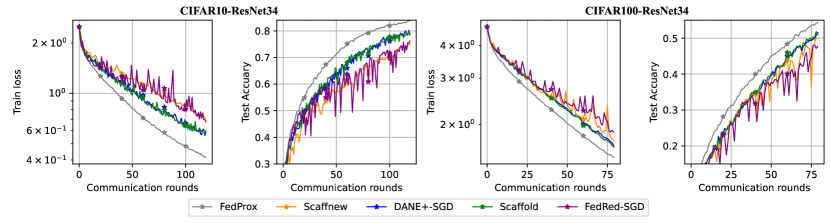
Figure C.1: Comparison of DANE+-SGD and FedRed-SGD against three other distributed optimizers on multi-class classification tasks with CIFAR10 and CIFAR100 datasets using ResNet18 with softmax loss. FedProx (without drift correction) exhibits faster and more stable convergence compared to the other methods.

References

- Acar et al. (2021) Durmus Alp Emre Acar, Yue Zhao, Ramon Matas, Matthew Mattina, Paul Whatmough, and Venkatesh Saligrama. Federated learning based on dynamic regularization. In International Conference on Learning Representations, 2021. URL https://openreview.net/forum?id=B7v4QMR6Z9w.
- Bubeck et al. (2015) Sébastien Bubeck et al. Convex optimization: Algorithms and complexity. Foundations and Trends® in Machine Learning, 8(3-4):231–357, 2015.
- Chang and Lin (2011) Chih-Chung Chang and Chih-Jen Lin. LIBSVM: A library for support vector machines. ACM Transactions on Intelligent Systems and Technology, 2:27:1–27:27, 2011. Software available at http://www.csie.ntu.edu.tw/~cjlin/libsvm.
- Condat and Richtárik (2022) Laurent Condat and Peter Richtárik. Randprox: Primal-dual optimization algorithms with randomized proximal updates. In OPT 2022: Optimization for Machine Learning (NeurIPS 2022 Workshop), 2022. URL https://openreview.net/forum?id=mejxBCu9EXc.
- Condat et al. (2023) Laurent Condat, Grigory Malinovsky, and Peter Richtárik. Tamuna: Accelerated federated learning with local training and partial participation. arXiv preprint arXiv:2302.09832, 2023.
- Defazio and Bottou (2019) Aaron Defazio and Léon Bottou. On the ineffectiveness of variance reduced optimization for deep learning. Advances in Neural Information Processing Systems, 32, 2019.
- Gao et al. (2022) Liang Gao, Huazhu Fu, Li Li, Yingwen Chen, Ming Xu, and Cheng-Zhong Xu. Feddc: Federated learning with non-iid data via local drift decoupling and correction. In Proceedings of the IEEE/CVF conference on computer vision and pattern recognition, pages 10112–10121, 2022.
- Grudzień et al. (2023) Michał Grudzień, Grigory Malinovsky, and Peter Richtárik. Can 5th generation local training methods support client sampling? yes! In International Conference on Artificial Intelligence and Statistics, pages 1055–1092. PMLR, 2023.
- He et al. (2016) Kaiming He, Xiangyu Zhang, Shaoqing Ren, and Jian Sun. Deep residual learning for image recognition. In 2016 IEEE Conference on Computer Vision and Pattern Recognition (CVPR), pages 770–778, 2016. doi: 10.1109/CVPR.2016.90.
- Hendrikx et al. (2020) Hadrien Hendrikx, Lin Xiao, Sebastien Bubeck, Francis Bach, and Laurent Massoulie. Statistically preconditioned accelerated gradient method for distributed optimization. In International conference on machine learning, pages 4203–4227. PMLR, 2020.
- Hu and Huang (2023) Zhengmian Hu and Heng Huang. Tighter analysis for ProxSkip. In Andreas Krause, Emma Brunskill, Kyunghyun Cho, Barbara Engelhardt, Sivan Sabato, and Jonathan Scarlett, editors, Proceedings of the 40th International Conference on Machine Learning, volume 202 of Proceedings of Machine Learning Research, pages 13469–13496. PMLR, 23–29 Jul 2023. URL https://proceedings.mlr.press/v202/hu23a.html.
- Kairouz et al. (2021) Peter Kairouz, H Brendan McMahan, Brendan Avent, Aurélien Bellet, Mehdi Bennis, Arjun Nitin Bhagoji, Kallista Bonawitz, Zachary Charles, Graham Cormode, Rachel Cummings, et al. Advances and open problems in federated learning. Foundations and Trends® in Machine Learning, 14(1–2):1–210, 2021.
- Karimireddy et al. (2020) Sai Praneeth Karimireddy, Satyen Kale, Mehryar Mohri, Sashank Reddi, Sebastian Stich, and Ananda Theertha Suresh. Scaffold: Stochastic controlled averaging for federated learning. In International conference on machine learning, pages 5132–5143. PMLR, 2020.
- Karimireddy et al. (2021) Sai Praneeth Karimireddy, Martin Jaggi, Satyen Kale, Mehryar Mohri, Sashank Reddi, Sebastian U. Stich, and Ananda Theertha Suresh. Breaking the centralized barrier for cross-device federated learning. In Advances in Neural Information Processing Systems, 2021.
- Khaled and Jin (2023) Ahmed Khaled and Chi Jin. Faster federated optimization under second-order similarity. In The Eleventh International Conference on Learning Representations, 2023. URL https://openreview.net/forum?id=ElC6LYO4MfD.
- Khaled et al. (2019) Ahmed Khaled, Konstantin Mishchenko, and Peter Richtárik. First analysis of local gd on heterogeneous data. arXiv preprint arXiv:1909.04715, 2019.
- Konečnỳ et al. (2016) Jakub Konečnỳ, H Brendan McMahan, Daniel Ramage, and Peter Richtárik. Federated optimization: Distributed machine learning for on-device intelligence. arXiv preprint arXiv:1610.02527, 2016.
- Kovalev et al. (2022) Dmitry Kovalev, Aleksandr Beznosikov, Ekaterina Borodich, Alexander Gasnikov, and Gesualdo Scutari. Optimal gradient sliding and its application to optimal distributed optimization under similarity. Advances in Neural Information Processing Systems, 35:33494–33507, 2022.
- Krizhevsky et al. (a) Alex Krizhevsky, Vinod Nair, and Geoffrey Hinton. Cifar-10 (canadian institute for advanced research). a. URL http://www.cs.toronto.edu/~kriz/cifar.html.
- Krizhevsky et al. (b) Alex Krizhevsky, Vinod Nair, and Geoffrey Hinton. Cifar-100 (canadian institute for advanced research). b. URL http://www.cs.toronto.edu/~kriz/cifar.html.
- Li et al. (2023) Bo Li, Mikkel N. Schmidt, Tommy S. Alstrøm, and Sebastian U. Stich. On the effectiveness of partial variance reduction in federated learning with heterogeneous data. In Proceedings of the IEEE/CVF Conference on Computer Vision and Pattern Recognition (CVPR), pages 3964–3973, June 2023.
- Li et al. (2020) Tian Li, Anit Kumar Sahu, Manzil Zaheer, Maziar Sanjabi, Ameet Talwalkar, and Virginia Smith. Federated optimization in heterogeneous networks. Proceedings of Machine learning and systems, 2:429–450, 2020.
- Lin et al. (2020) Tao Lin, Lingjing Kong, Sebastian U Stich, and Martin Jaggi. Ensemble distillation for robust model fusion in federated learning. Advances in Neural Information Processing Systems, 33:2351–2363, 2020.
- McMahan et al. (2017) Brendan McMahan, Eider Moore, Daniel Ramage, Seth Hampson, and Blaise Aguera y Arcas. Communication-efficient learning of deep networks from decentralized data. In Artificial intelligence and statistics, pages 1273–1282. PMLR, 2017.
- Mishchenko et al. (2022) Konstantin Mishchenko, Grigory Malinovsky, Sebastian Stich, and Peter Richtárik. Proxskip: Yes! local gradient steps provably lead to communication acceleration! finally! In International Conference on Machine Learning, pages 15750–15769. PMLR, 2022.
- Mitra et al. (2021) Aritra Mitra, Rayana Jaafar, George J. Pappas, and Hamed Hassani. Linear convergence in federated learning: Tackling client heterogeneity and sparse gradients. In A. Beygelzimer, Y. Dauphin, P. Liang, and J. Wortman Vaughan, editors, Advances in Neural Information Processing Systems, 2021. URL https://openreview.net/forum?id=h7FqQ6hCK18.
- Nasr et al. (2019) Milad Nasr, Reza Shokri, and Amir Houmansadr. Comprehensive privacy analysis of deep learning: Passive and active white-box inference attacks against centralized and federated learning. In 2019 IEEE symposium on security and privacy (SP), pages 739–753. IEEE, 2019.
- Nesterov (2018) Yurii Nesterov. Lectures on Convex Optimization. Springer Publishing Company, Incorporated, 2nd edition, 2018. ISBN 3319915770.
- Patel et al. (2022) Kumar Kshitij Patel, Lingxiao Wang, Blake Woodworth, Brian Bullins, and Nathan Srebro. Towards optimal communication complexity in distributed non-convex optimization. In Alice H. Oh, Alekh Agarwal, Danielle Belgrave, and Kyunghyun Cho, editors, Advances in Neural Information Processing Systems, 2022. URL https://openreview.net/forum?id=SNElc7QmMDe.
- Shamir et al. (2014) Ohad Shamir, Nati Srebro, and Tong Zhang. Communication-efficient distributed optimization using an approximate newton-type method. In Eric P. Xing and Tony Jebara, editors, Proceedings of the 31st International Conference on Machine Learning, volume 32 of Proceedings of Machine Learning Research, pages 1000–1008, Bejing, China, 22–24 Jun 2014. PMLR. URL https://proceedings.mlr.press/v32/shamir14.html.
- Sun et al. (2022) Ying Sun, Gesualdo Scutari, and Amir Daneshmand. Distributed optimization based on gradient tracking revisited: Enhancing convergence rate via surrogation. SIAM Journal on Optimization, 32(2):354–385, 2022.
- Tian et al. (2022) Ye Tian, Gesualdo Scutari, Tianyu Cao, and Alexander Gasnikov. Acceleration in distributed optimization under similarity. In International Conference on Artificial Intelligence and Statistics, pages 5721–5756. PMLR, 2022.
- Varno et al. (2022) Farshid Varno, Marzie Saghayi, Laya Rafiee Sevyeri, Sharut Gupta, Stan Matwin, and Mohammad Havaei. Adabest: Minimizing client drift in federated learning via adaptive bias estimation. In European Conference on Computer Vision, pages 710–726. Springer, 2022.
- Wang et al. (2018) Shusen Wang, Fred Roosta, Peng Xu, and Michael W Mahoney. Giant: Globally improved approximate newton method for distributed optimization. Advances in Neural Information Processing Systems, 31, 2018.
- Woodworth et al. (2020) Blake E Woodworth, Kumar Kshitij Patel, and Nati Srebro. Minibatch vs local sgd for heterogeneous distributed learning. Advances in Neural Information Processing Systems, 33:6281–6292, 2020.
- Yuan and Li (2019) Xiao-Tong Yuan and Ping Li. On convergence of distributed approximate newton methods: Globalization, sharper bounds and beyond. arXiv preprint arXiv:1908.02246, 2019.
- Zhang et al. (2021) Xinwei Zhang, Mingyi Hong, Sairaj Dhople, Wotao Yin, and Yang Liu. Fedpd: A federated learning framework with adaptivity to non-iid data. IEEE Transactions on Signal Processing, 69:6055–6070, 2021.
- Zhang and Lin (2015) Yuchen Zhang and Xiao Lin. Disco: Distributed optimization for self-concordant empirical loss. In Francis Bach and David Blei, editors, Proceedings of the 32nd International Conference on Machine Learning, volume 37 of Proceedings of Machine Learning Research, pages 362–370, Lille, France, 07–09 Jul 2015. PMLR. URL https://proceedings.mlr.press/v37/zhangb15.html.
- Zindari et al. (2023) Ali Zindari, Ruichen Luo, and Sebastian U Stich. On the convergence of local SGD under third-order smoothness and hessian similarity. In OPT 2023: Optimization for Machine Learning, 2023. URL https://openreview.net/forum?id=OnJa9N4VwY.