MSSTNet: A Multi-Scale Spatio-Temporal CNN-Transformer Network for Dynamic Facial Expression Recognition
Abstract
Unlike typical video action recognition, Dynamic Facial Expression Recognition (DFER) does not involve distinct moving targets but relies on localized changes in facial muscles. Addressing this distinctive attribute, we propose a Multi-Scale Spatio-temporal CNN-Transformer network (MSSTNet). Our approach takes spatial features of different scales extracted by CNN and feeds them into a Multi-scale Embedding Layer (MELayer). The MELayer extracts multi-scale spatial information and encodes these features before sending them into a Temporal Transformer (T-Former). The T-Former simultaneously extracts temporal information while continually integrating multi-scale spatial information. This process culminates in the generation of multi-scale spatio-temporal features that are utilized for the final classification. Our method achieves state-of-the-art results on two in-the-wild datasets. Furthermore, a series of ablation experiments and visualizations provide further validation of our approach’s proficiency in leveraging spatio-temporal information within DFER.
Index Terms— Dynamic facial expression recognition, Affective Computing, Transformer, Spatio-temporal dependencies
1 Introduction
Facial expression recognition (FER) finds extensive applications in daily life, such as affective computing, human-computer interaction, fatigue detection in driving, and emotional robots, among others [1]. Dynamic Facial Expression Recognition (DFER) aims to recognize emotions within a video segment, which typically yields more precise results than single static images.
Traditional DFER methods rely on manual feature extraction techniques, such as LBP-TOP [2], STLMBP [3], and HOG-TOP [4]. With the rise of deep learning, models based on deep learning have emerged as the mainstream approach in the DFER domain. These approaches utilize the Convolutional Neural Network (CNN) to extract image features, followed by modeling of the temporal sequences through models like Recurrent Neural Network (RNN) [5, 6], Long Short-Term Memory (LSTM) [7], or Gated Recurrent Unit (GRU) [8]. Additionally, 3D CNNs [9] are commonly employed for DFER as they can simultaneously capture spatial and temporal features. In recent years, the Transformer [10] architecture, which has achieved significant success in the Natural Language Processing (NLP) field, has gradually been introduced to computer vision. Its global attention mechanism and parallel computing capabilities are effective for modeling time sequences. Consequently, an increasing number of researchers are incorporating transformers into DFER [11, 12], and some even explore their use in methods designed for video action recognition [13, 14, 15].
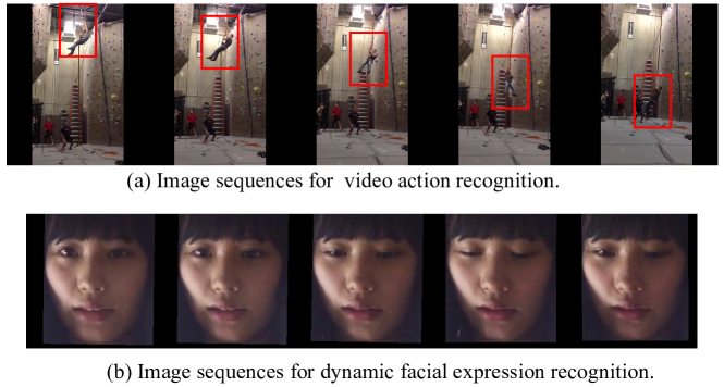
However, unlike typical video action recognition, DFER does not involve clearly moving targets. As depicted in Figure 1(a), video action recognition often deals with prominently shifting targets. In contrast, in the context of DFER, as illustrated in Figure 1(b), the image sequences typically undergo facial alignment preprocessing. Consequently, there are no moving targets; instead, the variations observed are in the state of facial muscles over time [16].
In response to these characteristics, we propose the Multi-Scale Spatio-temporal CNN-Transformer Network (MSSTNet). We introduce a novel Multi-scale Embedding Layer (MELayer), which encodes spatial features of varying sizes extracted by the CNN, and subsequently feeds them into the Temporal Transformer (T-Former). The T-Former, while extracting temporal information, simultaneously integrates spatial information of different scales, culminating in the generation of multi-scale spatio-temporal features. Our method achieves state-of-the-art performance on two widely-used in-the-wild DFER datasets. A series of ablation experiments and visualizations provide empirical evidence of the effectiveness of the spatio-temporal features generated by our approach.
2 The Proposed Method
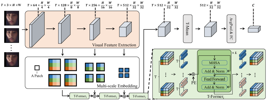
The overall architecture of our approach is depicted in Figure 2. Given an image sequence with RGB facial frames of size , we employ a CNN backbone to extract visual features of varying scales, including spatial positional information. The MELayer encodes these features and passes them to the T-Former. The T-Former utilizes the encoder architecture from the Transformer to extract temporal information while concurrently integrating multi-scale spatial information. The T-Former’s output is subjected to temporal and spatial dimension-wise averaging, followed by a fully connected network, to obtain the final classification result.
2.1 Multi-scale Embedding Layer (MELayer)
The MELayer takes feature maps of varying sizes and encodes each of them into patches. A particular input denoted as , comprising feature maps, with each feature map having channels and spatial dimensions . We decompose each feature map into non-overlapping patches, each of size , such that the patches span the entire frame, i.e., . We flatten these patches into vectors with denoting spatial locations and depicting an index over frames. We linearly map each patch into an embedding vector by means of a learnable matrix :
| (1) |
where represents a learnable temporal positional embedding. It’s worth noting that spatial positional embeddings are not included here. Since the T-Former treats the same region as tokens, spatial positional embedding is unnecessary. Consequently, in this context, only temporal position embeddings are introduced. The resulting sequence of embedding vectors represents the input to the T-Former.
2.2 Temporal Transformer (T-Former)
The T-Former consists of Transformer encoding blocks, designed to extract temporal features of the same region at different time points while progressively integrating multi-scale spatial information.
Query-Key-Value Computation. At each block , a query/key/value vector is computed for each patch from the representation encoded by the preceding block:
| (2) | ||||
| (3) | ||||
| (4) |
where denotes LayerNorm, is an index over multiple attention heads and denotes the total number of attention heads. The latent dimensionality for each attention head is set to .
Self-attention Computation. Self-attention weights are computed via dot-product. The self-attention weights for query patch are given by:
| (5) |
where denotes the softmax activation function. It’s worth noting that in our approach, we exclusively compute self-attention in the temporal dimension. This choice results in a significant reduction in computational cost compared to simultaneously computing attention in both spatial and temporal dimensions.
Encoding. The encoding at block is obtained by first computing the weighted sum of value vectors using self-attention coefficients from each attention head:
| (6) |
Then, the concatenation of these vectors from all heads is projected and passed through an MLP, using residual connections after each operation:
| (10) | ||||
| (11) |
All the features produced by the final block, denoted as are averaged across both the temporal and spatial dimensions to obtain , followed by further processing through a fully connected (FC) layer to obtain the final result.
| (12) |
where is the prediction distribution of facial expression classes.
| T-Former1 | T-Former2 | T-Former3 | WAR(%) | ||
| FERV39k | DFEW | ||||
| 4 | 46.89 | 65.91 | |||
| 47.83 | 66.68 | ||||
| 48.08 | 67.93 | ||||
| 48.42 | 68.37 | ||||
| 1 | 1 | 1 | 49.94 | 68.97 | |
| 2 | 2 | 2 | 49.89 | 69.71 | |
| 3 | 3 | 3 | 49.11 | 69.36 | |
| 8 | 1 | 1 | 1 | 49.66 | 69.89 |
| 2 | 2 | 2 | 50.25 | 70.16 | |
| 3 | 3 | 3 | 49.29 | 69.65 | |
| 12 | 1 | 1 | 1 | 49.97 | 70.53 |
| 2 | 2 | 2 | 50.43 | 70.85 | |
| 3 | 3 | 3 | 50.01 | 70.31 | |
| 16 | 1 | 1 | 1 | 50.17 | 70.81 |
| 2 | 2 | 2 | 51.02 | 71.42 | |
| 3 | 3 | 3 | 50.42 | 70.99 | |
| Method | Metrics(%) | |
|---|---|---|
| WAR | UAR | |
| R18-LSTM[17, 7, 18] | 42.59 | 30.92 |
| VGG13-LSTM[19, 7, 18] | 43.37 | 32.41 |
| C3D[20, 18] | 31.69 | 22.68 |
| 3D ResNet18[21, 18] | 37.57 | 26.67 |
| Former-DFER[11] | 45.72 | 36.88 |
| LOGO-Former[16] | 48.13 | 38.22 |
| MSSTNetT=4(Ours) | 49.89 | 39.80 |
| MSSTNetT=8(Ours) | 50.25 | 40.46 |
| MSSTNetT=12(Ours) | 50.43 | 40.70 |
| MSSTNetT=16(Ours) | 51.02 | 41.28 |
| Method | Accuracy of Each Emotion (%) | Metrics (%) | FLOPs | |||||||
| Happy | Sad | Neutral | Angry | Surprise | Disgust | Fear | UAR | WAR | (G) | |
| R(2+1)D18 [21] | 79.67 | 39.07 | 57.66 | 50.39 | 48.26 | 3.45 | 21.06 | 42.79 | 53.22 | 42.36 |
| 3D Resnet18 [22] | 73.13 | 48.26 | 50.51 | 64.75 | 50.10 | 0.00 | 26.39 | 44.73 | 54.98 | 8.32 |
| ResNet18+LSTM [7, 17] | 78.00 | 40.65 | 53.77 | 56.83 | 45.00 | 4.14 | 21.62 | 42.86 | 53.08 | 7.78 |
| Resnet18+GRU [17, 8] | 82.87 | 63.83 | 65.06 | 68.51 | 52.00 | 0.86 | 30.14 | 51.68 | 64.02 | 7.78 |
| Former-DFER [11] | 84.05 | 62.57 | 67.52 | 70.03 | 56.43 | 3.45 | 31.78 | 53.69 | 65.70 | 9.11 |
| DPCNet [23] | - | - | - | - | - | - | - | 57.11 | 66.32 | 9.52 |
| NR-DFERNet [12] | 86.42 | 65.10 | 70.40 | 72.88 | 50.10 | 0.00 | 45.44 | 55.77 | 68.01 | 6.33 |
| LOGO-Former [16] | 85.39 | 66.52 | 68.94 | 71.33 | 54.59 | 0.00 | 32.71 | 54.21 | 66.98 | 10.27 |
| MSSTNetT=4(Ours) | 89.57 | 71.28 | 69.01 | 70.92 | 55.89 | 11.03 | 43.68 | 58.77 | 69.71 | 5.05 |
| MSSTNetT=8(Ours) | 89.20 | 70.12 | 72.35 | 70.23 | 59.22 | 13.10 | 39.02 | 59.04 | 70.16 | 10.10 |
| MSSTNetT=12(Ours) | 90.22 | 70.22 | 70.93 | 74.60 | 59.50 | 10.34 | 38.58 | 59.20 | 70.85 | 15.15 |
| MSSTNetT=16(Ours) | 90.39 | 71.54 | 71.94 | 73.17 | 61.20 | 13.79 | 39.91 | 60.28 | 71.42 | 20.20 |
3 Experiments
We conducted experiments on two widely-used real-world datasets: DFEW [24] and FERV39k [18], both of which provide images that have undergone official facial alignment processing. We employed the Weighted Average Recall (WAR) and the Unweighted Average Recall (UAR) as evaluation metrics. Following prior research [11, 12, 16], we utilized ResNet-18 as the CNN backbone. In the T-Former architecture, we configured the feature dimension , number of patches and number of heads as 768, 16 and 8, respectively. All our models were implemented using PyTorch and trained on an NVIDIA TITAN RTX GPU. The training process employed the SGD optimizer with an initial learning rate of 0.1 for 40 epochs. Learning rate decay by a factor of 10 occurred at the 20th and 35th epochs.
Ablation Studies. We evaluated the impact of various components of MSSTNet, and the experimental results are presented in Table 1. Each stage of the T-Former contributes to an enhancement in model performance, affirming the T-Former’s proficiency in capturing temporal features. Notably, the combined interaction of all T-Former stages yields the greatest improvement in model performance, underscoring the effectiveness of multi-scale spatio-temporal features. Moreover, merely increasing the number of T-Former blocks does not lead to improved performance; instead, it introduces additional computational complexity. As a result, we set the number of blocks to 2 in subsequent experiments. Furthermore, the model’s performance improves with an increase in the number of input frames, validating the efficacy of our approach in modeling the temporal dimension.
Comparison with State-of-the-Art Methods. The comparative analysis between our method and others on the two datasets is presented in Tables 2 and 3. Our approach outperforms previous methods on both datasets, regardless of the number of input frames. On the DFEW dataset, MSSTNet outperforms the previous best method with significant improvements of 3.41% in WAR and 3.17% in UAR, with a notable 9.65% increase in accuracy for the disgust category. Furthermore, MSSTNet marks a pioneering achievement as the first method to attain a WAR of over 70%. On the FERV39k dataset, our method also establishes a new benchmark by achieving a WAR exceeding 50%. It surpasses the previous best method with improvements of 2.89% in WAR and 3.06% in UAR.
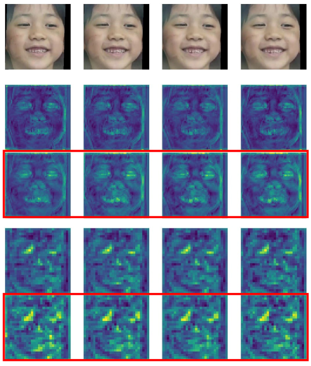
Visualization. To evaluate the effectiveness of the T-Former in our approach, we conducted feature map visualizations as shown in Figure 3. The visualized outcomes reveal that, compared to feature maps without the T-Former, those processed by the T-Former demonstrate a clear focus on regions that reflect facial muscles variations, such as the eyes, nose, and mouth. This observation underscores the robust global temporal feature extraction capability of the T-Former, contributing to the model’s enhanced performance.
4 Conclusion
In this paper, we address the dynamic variations within localized facial muscle regions in DFER by proposing a Multi-Scale Spatio-temporal CNN-Transformer network (MSSTNet). Our approach leverages CNN to capture spatial information, while Multi-scale Embedding Layer (MELayer) focuses on features within localized regions experiencing variations. Furthermore, a Temporal Transformer (T-Former) is employed to extract temporal information and integrate it with multi-scale spatial information, ultimately yielding multi-scale spatio-temporal features. Importantly, our method achieves state-of-the-art results on two commonly used in-the-wild datasets. Ablation experiments and visualizations further substantiate the effectiveness of our approach.
References
- [1] Linhuang Wang, Xin Kang, Satoshi Nakagawa, and Fuji Ren, “Centermatch: A center matching method for semi-supervised facial expression recognition,” in Chinese Conference on Pattern Recognition and Computer Vision. Springer, 2023, pp. 371–383.
- [2] Abhinav Dhall, Roland Goecke, Jyoti Joshi, Michael Wagner, and Tom Gedeon, “Emotion recognition in the wild challenge 2013,” in Proceedings of the 15th ACM on International conference on multimodal interaction, 2013, pp. 509–516.
- [3] Xiaohua Huang, Qiuhai He, Xiaopeng Hong, Guoying Zhao, and Matti Pietikainen, “Improved spatiotemporal local monogenic binary pattern for emotion recognition in the wild,” in Proceedings of the 16th International Conference on Multimodal Interaction, 2014, pp. 514–520.
- [4] JunKai Chen, Zenghai Chen, Zheru Chi, and Hong Fu, “Emotion recognition in the wild with feature fusion and multiple kernel learning,” in Proceedings of the 16th International Conference on Multimodal Interaction, 2014, pp. 508–513.
- [5] Yanan Wang, Jianming Wu, and Keiichiro Hoashi, “Multi-attention fusion network for video-based emotion recognition,” in 2019 International Conference on Multimodal Interaction, 2019, pp. 595–601.
- [6] Samira Ebrahimi Kahou, Vincent Michalski, Kishore Konda, Roland Memisevic, and Christopher Pal, “Recurrent neural networks for emotion recognition in video,” in Proceedings of the 2015 ACM on international conference on multimodal interaction, 2015, pp. 467–474.
- [7] Sepp Hochreiter and Jürgen Schmidhuber, “Long short-term memory,” Neural computation, vol. 9, no. 8, pp. 1735–1780, 1997.
- [8] Junyoung Chung, Caglar Gulcehre, KyungHyun Cho, and Yoshua Bengio, “Empirical evaluation of gated recurrent neural networks on sequence modeling,” arXiv preprint arXiv:1412.3555, 2014.
- [9] Yin Fan, Xiangju Lu, Dian Li, and Yuanliu Liu, “Video-based emotion recognition using cnn-rnn and c3d hybrid networks,” in Proceedings of the 18th ACM international conference on multimodal interaction, 2016, pp. 445–450.
- [10] Ashish Vaswani, Noam Shazeer, Niki Parmar, Jakob Uszkoreit, Llion Jones, Aidan N Gomez, Lukasz Kaiser, and Illia Polosukhin, “Attention is all you need,” Advances in neural information processing systems, vol. 30, 2017.
- [11] Zengqun Zhao and Qingshan Liu, “Former-dfer: Dynamic facial expression recognition transformer,” in Proceedings of the 29th ACM International Conference on Multimedia, 2021, pp. 1553–1561.
- [12] Hanting Li, Mingzhe Sui, Zhaoqing Zhu, et al., “Nr-dfernet: Noise-robust network for dynamic facial expression recognition,” arXiv preprint arXiv:2206.04975, 2022.
- [13] Gedas Bertasius, Heng Wang, and Lorenzo Torresani, “Is space-time attention all you need for video understanding?,” in ICML, 2021, vol. 2, p. 4.
- [14] Shuyan Li, Xiu Li, Jiwen Lu, and Jie Zhou, “Self-supervised video hashing via bidirectional transformers,” in Proceedings of the IEEE/CVF Conference on Computer Vision and Pattern Recognition, 2021, pp. 13549–13558.
- [15] Guangming Wang, Hanwen Liu, Muyao Chen, Yehui Yang, Zhe Liu, and Hesheng Wang, “Anchor-based spatio-temporal attention 3-d convolutional networks for dynamic 3-d point cloud sequences,” IEEE Transactions on Instrumentation and Measurement, vol. 70, pp. 1–11, 2021.
- [16] Fuyan Ma, Bin Sun, and Shutao Li, “Logo-former: Local-global spatio-temporal transformer for dynamic facial expression recognition,” in ICASSP 2023-2023 IEEE International Conference on Acoustics, Speech and Signal Processing (ICASSP). IEEE, 2023, pp. 1–5.
- [17] Kaiming He, Xiangyu Zhang, Shaoqing Ren, and Jian Sun, “Deep residual learning for image recognition,” in Proceedings of the IEEE conference on computer vision and pattern recognition, 2016, pp. 770–778.
- [18] Yan Wang, Yixuan Sun, Yiwen Huang, Zhongying Liu, Shuyong Gao, Wei Zhang, Weifeng Ge, and Wenqiang Zhang, “Ferv39k: A large-scale multi-scene dataset for facial expression recognition in videos,” in Proceedings of the IEEE/CVF conference on computer vision and pattern recognition, 2022, pp. 20922–20931.
- [19] Karen Simonyan and Andrew Zisserman, “Very deep convolutional networks for large-scale image recognition,” arXiv preprint arXiv:1409.1556, 2014.
- [20] Du Tran, Lubomir Bourdev, Rob Fergus, Lorenzo Torresani, and Manohar Paluri, “Learning spatiotemporal features with 3d convolutional networks,” in Proceedings of the IEEE international conference on computer vision, 2015, pp. 4489–4497.
- [21] Du Tran, Heng Wang, Lorenzo Torresani, Jamie Ray, Yann LeCun, and Manohar Paluri, “A closer look at spatiotemporal convolutions for action recognition,” in Proceedings of the IEEE conference on Computer Vision and Pattern Recognition, 2018, pp. 6450–6459.
- [22] Kensho Hara, Hirokatsu Kataoka, and Yutaka Satoh, “Can spatiotemporal 3d cnns retrace the history of 2d cnns and imagenet?,” in Proceedings of the IEEE conference on Computer Vision and Pattern Recognition, 2018, pp. 6546–6555.
- [23] Yan Wang, Yixuan Sun, Wei Song, Shuyong Gao, Yiwen Huang, Zhaoyu Chen, Weifeng Ge, and Wenqiang Zhang, “Dpcnet: Dual path multi-excitation collaborative network for facial expression representation learning in videos,” in Proceedings of the 30th ACM International Conference on Multimedia, 2022, pp. 101–110.
- [24] Xingxun Jiang, Yuan Zong, Wenming Zheng, Chuangao Tang, Wanchuang Xia, Cheng Lu, and Jiateng Liu, “Dfew: A large-scale database for recognizing dynamic facial expressions in the wild,” in Proceedings of the 28th ACM international conference on multimedia, 2020, pp. 2881–2889.