PiRD: Physics-informed Residual Diffusion
for Flow Field Reconstruction
Abstract
The use of machine learning in fluid dynamics is becoming more common to expedite the computation when solving forward and inverse problems of partial differential equations. Yet, a notable challenge with existing convolutional neural network (CNN)-based methods for data fidelity enhancement is their reliance on specific low-fidelity data patterns and distributions during the training phase. In addition, the CNN-based method essentially treats the flow reconstruction task as a computer vision task that prioritizes the element-wise precision which lacks a physical and mathematical explanation. This dependence can dramatically affect the models’ effectiveness in real-world scenarios, especially when the low-fidelity input deviates from the training data or contains noise not accounted for during training. The introduction of diffusion models in this context shows promise for improving performance and generalizability. Unlike direct mapping from a specific low-fidelity to a high-fidelity distribution, diffusion models learn to transition from any low-fidelity distribution towards a high-fidelity one. Our proposed model - Physics-informed Residual Diffusion, demonstrates the capability to elevate the quality of data from both standard low-fidelity inputs, to low-fidelity inputs with injected Gaussian noise, and randomly collected samples. By integrating physics-based insights into the objective function, it further refines the accuracy and the fidelity of the inferred high-quality data. Experimental results have shown that our approach can effectively reconstruct high-quality outcomes for two-dimensional turbulent flows from a range of low-fidelity input conditions without requiring retraining.
1 Introduction
As a typical inverse problem, reconstructing spatial fields from sparse sensor data is a highly challenging task, yet its applications are widespread, encompassing numerous fields such as medicine, industrial devices, remote sensing, fluid dynamics, and more [1, 2, 3, 4]. Efforts to improve traditional methodologies for effectively handling sparse input data have to face a balance between computational efficiency and effectiveness [5]. Meanwhile, due to the potential movement and loss of sparse sensors, the fidelity of experimental setups utilizing these collected data is inevitably affected, which leads to structural instability [6]. Moreover, the noise introduced by the sensor measurement process cannot be ignored. All these aspects lead to a complex challenge for reconstruction, which is difficult to meet by traditional methods.
In fluid dynamics, Direct Numerical Simulation (DNS) is a classic method that simulates fluid motion directly by solving the complete Navier-Stokes equations in all scales. To obtain high-fidelity flow field information, DNS requires significant computational resources, especially when solving ill-posed problems or inverse problems related to turbulent flows. Indeed, owing to computational efficiency challenges, several methods employing simplified turbulence models for approximate calculations have been devised, such as Large Eddy Simulation (LES) [7], Reynolds-Averaged Navier-Stokes (RANS) models [8] and hybrid RANS-LES approaches [9]. Nonetheless, these approaches require a trade-off between accuracy and computational expedience. In addition, data assimilation algorithms are proposed to integrate the measurements with the aforementioned numerical models. For example, Wang et al.[10, 11] introduced an adjoint-variational data-assimilation algorithm to reconstruct the flow fields from measurements and enhance traditional methods in the sparse condition. However, these methods also suffer from computational inefficiency, requiring iterative solutions to the Navier-Stokes equations. To mitigate the conflicts between computational cost and simulation accuracy, we aim to draw insights from end-to-end models designed for rapid inference to bridge the gap between simulations and real-world flow field environments, which have demonstrated success in diverse applications such as image processing.
In the field of image processing, the use of machine learning for super-resolution enhancement and data recovery techniques from low-resolution or sparse pixel points is developing rapidly, including algorithms based on convolutional neural networks (CNN) [12, 13], transformer architectures [14, 15, 16], and generative adversarial networks (GAN) [17, 18, 19]. While super-resolution is generally regarded as an image-based data recovery technique, these neural network frameworks have been widely applied to fluid mechanics [20, 21, 22, 23, 24], providing promising alternatives to traditional methods.
Despite the considerable achievements gained by CNN-based methodologies in enhancing the resolution of specific low-fidelity image distributions, they share a common limitation: these models are intricately designed and fine-tuned for a distinct class of under-resolved flow field data, heavily reliant on their training data characteristics. In contrast, real-world flow field scenarios present a far more complex and unpredictable landscape. Sensor placement is often sparse and varied, and the data acquired is frequently contaminated with noise. Such conditions inevitably result in discrepancies between training datasets and real-world testing scenarios. This limitation presents challenges in the generalization and robustness of CNN-based models, restricting their applicability in real-world environments.
Revisiting techniques from the field of image reconstruction, if we regard sparse low-resolution fluid flow data as noisy experimental measurements, then super-resolution flow field reconstruction can be considered as a natural denoising problem. Therefore, the diffusion model in the generation problem [25, 26, 27] also has the potential to reconstruct the sparse data flow field. In this context, Shu et al. [28] introduced a model based on the Diffusion Probabilistic Model (DDPM) for super-resolution tasks, demonstrating its versatility across various scenarios to overcome the limitations in the CNN-based model used in fluid dynamics.
However, due to the denoising nature of DDPM-based models, rather than incorporating physics-informed constraints directly into the objective function, a physics-conditioning embedding is applied during the training phase. This approach allows the model to correct physics deviations in the denoised flow field iteratively during the sampling phase. Although effective, the reliance on the number of sampling steps to achieve minimal partial differential equation loss may inadvertently compromise the efficiency of the algorithm. This introduces the need for fine-tuning certain hyperparameters for specific datasets to achieve accurate results, potentially straying from the original intent of developing such models. Moreover, despite the integration of physical condition embedding, the flow field reconstructed using DDPM occasionally fails to comply with the physical constraints on a localized scale.
To tackle these challenges, we propose a residual-based diffusion model for flow field super-resolution in this work, inspired by Yue et al.[29] where a diffusion model with residual shifting was presented. Unlike traditional DDPM-based methods, the residual-based diffusion model requires fewer sampling steps and predicts the original high-fidelity flow field directly. This approach enables the practical application of Physics-Informed Neural Networks (PINNs) by integrating the residuals of the governing equations within the objective function, leading to a brand new model called physics-informed residual diffusion (PiRD) model in this paper. Our model not only demonstrates robust performance in reconstructing low-fidelity data across a variety of conditions in the turbulence experiment, but also enhances both training and sampling efficiency—requiring approximately 20 epochs for training and 20 steps for sampling.
Contributions: We make the following key contributions: (i) We present a novel, effective and motivated approach that embeds physical information into the diffusion model to solve the problem of flow field reconstruction under sparse and noisy measurements. (ii) Due to the nature of the ResShift diffusion model, our proposed method can complete the training or inference in about 20 steps, which greatly improves the calculation speed compared with [28], and it is beneficial for future application to actual real-time flow field scenarios. (iii) Through some classical turbulence experiments, PiRD is proved to be more accurate and robust than the CNN-based model for flow field reconstruction on sparse data. Moreover, PiRD can handle various sensor placements and noisy measurements which are not considered in the training data.
2 Methods
2.1 Problem Setup
The primary objective of this research is to address the limitations of current CNN-based methods in reconstructing high-fidelity (HF) flow fields, denoted as , from low-fidelity (LF) observations, denoted as . Conventional CNN-based models like UNet, represented as , have shown proficiency in dealing with in-distribution low-fidelity data. This process can be described as:
where represents certain the down-sampling operation, or a certain method to degrade the high-fidelity flow field, the neural network is essentially trying to learn this operation to reserve this process, and in-distribution data means the high-fidelity data that was corrupted by this down-sampling operation , or in which operations that are highly similar to it. However, the learned model can only be applicable for the scenarios that are degraded by this specific learned , if the degraded flow field is not corrupted by it, the reconstruction process still trying to reverse which ultimately make the prediction inaccurate. Therefore, to address this problem, we build up a Markov chain between high-fidelity flow fields and low-fidelity flow fields that are independent of , such that we can reconstruct low-fidelity flow fields given any possible . In addition, physics-informed loss function can also be integrated into such a process to act as not only a physical constraint to make sure that the prediction follows the underlying physical law, but also a guide for the model to infer the information lost in the low-fidelity flow field and ensure robust performance across diverse and challenging scenarios.
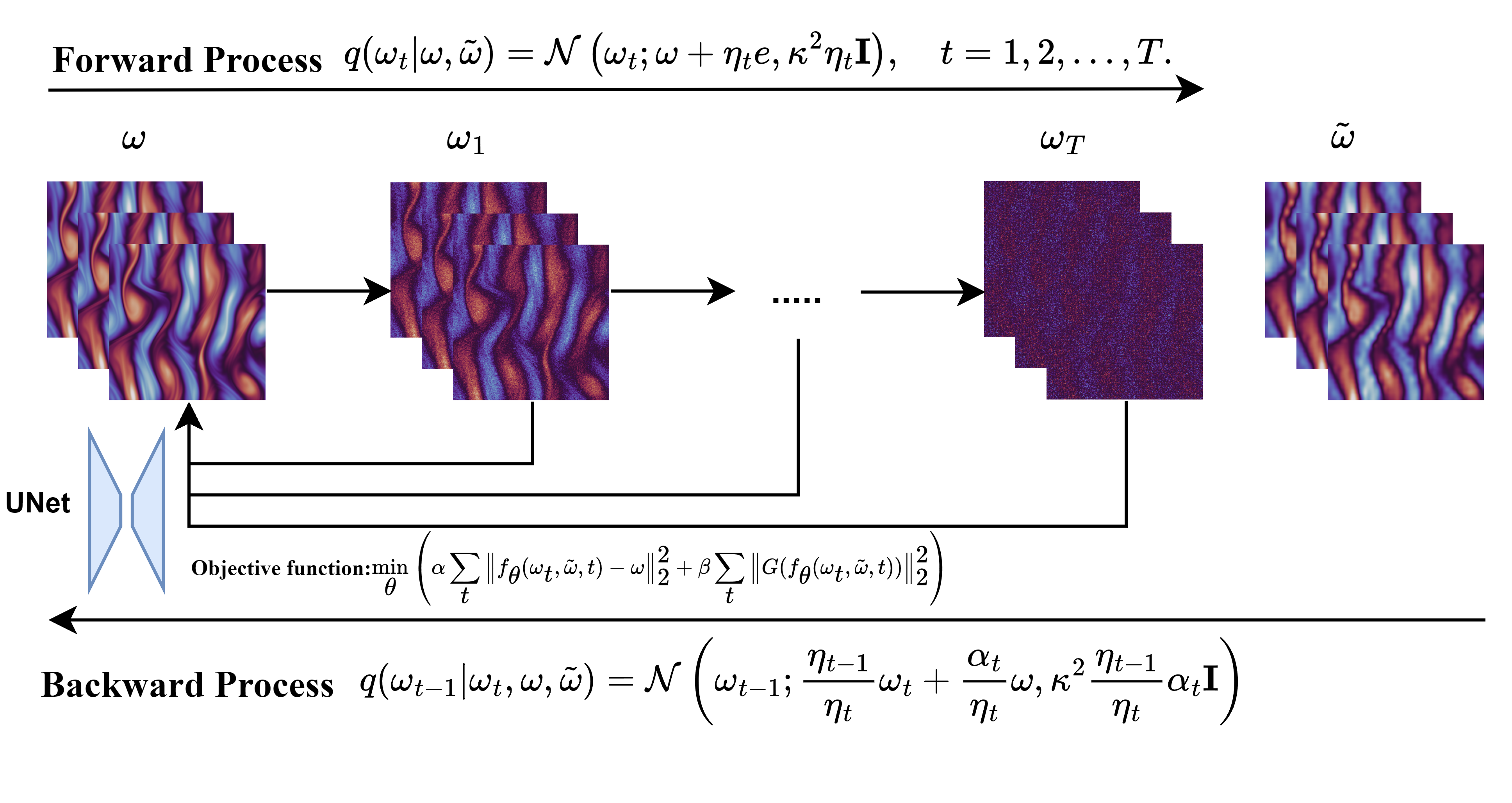
2.2 Physics-informed Residual Diffusion
This section introduces our proposed model used to map the low-fidelity distribution to the high-fidelity distribution through a learned Markov chain and to ensure that the entire process follows the underlying physical law such that we can eventually produce a high-fidelity prediction that also obeys the physical law. In the following, we present the architecture of Physics-informed Residual Diffusion (PiRD) which is composed of two essential modules: (i) Residual Shifting Diffusion Model that could build a Markov chain between LF distributions and HF distributions; (ii) Physics-informed neural networks(PINNs) for fluid mechanics that ensure the predictions obey the underlying physical law.
2.2.1 Residual Shifting Diffusion Model for Vorticity Field
Residual Shifting Diffusion Model was first proposed by Yue et al. [29] developed for the image super-resolution task. This method diverges from traditional approaches that transition high-fidelity images to Gaussian noise. Instead, it constructs a Markov chain between high-resolution images and low-resolution images, facilitated by adjusting the residual between them. We apply this method as the backbone of our task, expand this ideal and further develop this idea into the application of low-fidelity flow field super-resolution and sparse flow field reconstruction. Let denoted as the high-fidelity flow field, ad as its corresponding low-fidelity flow field, and let denoted the residual between them, this residual does not only contains the spatially related difference between them but also contains the physical related information lost between them. The forward diffusion Markov chain can be described as:
| (1) | ||||
| (2) |
where is a shifting schedule that increases with the time step such that a smooth transition of to over a sequence of steps can be built. for and , is the key parameter that controls the progression of noise variance. Therefore the reverse process estimates the posterior distribution using:
| (3) |
Since in the forward diffusion process we have defined , and 1 we can approximate where , consequently, we can also approximate ) by . is the reverse transition kernel. By minimizing the negative evidence lower bound to make tractable, we can get below representations:
| (4) |
| (5) |
The above reverse transition kernel shows that for each iterative backward process, we need the original high-fidelity flow field to infer from to , therefore the objective function can be designed as follows:
| (6) |
2.2.2 Physics-informed neural networks (PINNs) for fluid mechanics
Within the realm of fluid mechanics, the application of Physics-Informed Neural Networks (PINNs) to the vorticity transport equations exemplifies a sophisticated methodology for solving parametrized partial differential equations (PDEs) that describe complex fluid behaviours. The vorticity transport equation, pivotal for understanding fluid dynamics, models the evolution of vorticity , a vector field that characterizes the local spinning motion of the fluid. This equation is succinctly represented as
| (7) |
where denotes the velocity field, the kinematic viscosity.
This equation embodies the conservation of vorticity in the absence of external influences and lays the foundation for the application of PINNs in fluid mechanics.
The PINNs framework for solving the vorticity transport equation integrates the physics of the problem directly into the learning process of the neural network. By approximating the solution , the network is trained to comply with the governing PDE across the domain and throughout the time interval . This training process is facilitated by the formulation of a composite loss function , which encapsulates the adherence of the network’s output to the underlying physical laws and empirical data. The loss function is articulated as
| (8) |
where each term represents a different aspect of the learning criteria: penalizes deviations from the vorticity transport PDE, quantifies the discrepancies between the predictions and actual flow measurements, and ensure the model’s output matches the initial and boundary conditions, respectively, denotes the weighting coefficient for each term. To integrate the initial and boundary conditions crucial for accurately modeling fluid behaviour, PINNs incorporate these conditions directly into the loss function. Initial conditions set the stage for the fluid’s state at the beginning of the observation period, whereas boundary conditions dictate the fluid’s behaviour at the domain’s edges, influencing the evolution of the flow over time. The precise specification of these conditions is vital for capturing the physical scenario under investigation, such as the generation and dynamics of vorticity in flows past obstacles.
An adaptive optimization algorithm, typically ADAM, is employed to minimize the loss function. This optimization approach adjusts the learning rate dynamically, enabling efficient convergence towards a parameter set that best represents the solution to the vorticity transport equation while respecting both the fluid dynamics and the available empirical data.
2.2.3 Physics-informed Residual Diffusion
The traditional Residual Diffusion Model (RDM) operates by constructing a Markov chain, characterizing a residual, , that bridges the gap between the high-fidelity vorticity field, , and its low-fidelity counterpart, . This residual is dissected into two principal components: , which represents the element-wise discrepancies, and , which captures deviations from established physical laws. Consequently, the transformation process from to is encapsulated by the equation:
| (9) |
While plays a pivotal role in enhancing resolution, effectively addressing poses a significant challenge due to the complex nature of fluid dynamics, and flow field reconstruction cannot be simply seen as a mere computer vision task, which prioritizes the pixel-wise similarity. In many scenarios, it is possible that for a pair of predictions with the same pixel-wise mean relative error compared to the ground truth, their respective prediction has large differences in terms of physics property. Therefore, if the Markov chain could facilitate the inference of a high-fidelity (HF) vorticity field from a low-fidelity (LF) one while rigorously adhering to physical laws, the flow field reconstructed could make sure that it not only revert but also . Nonetheless, realizing this ideal scenario requires two often unattainable conditions in practical applications: (i) the presence of ample training data to thoroughly represent Markov chain transitions. (ii) LF distribution representations at the termination of the chain () that accurately reflect all conceivable LF situations, crucial for recovering .
To address these challenges, we introduce Physics-informed Residual Diffusion (PiRD). PiRD enriches the RDM framework by embedding physics-informed constraints within the model’s loss function, ensuring adherence to physical laws at every step of the Markov chain. This approach serves a dual purpose: it acts as a form of data augmentation, introducing crucial information for model learning, and it can also guarantee that each LF vorticity field is transitioned towards the HF distribution in compliance with physical principles without the concern that the physics-wise error will accumulate during the sampling process. Through this integration, PiRD can effectively map complex LF vorticity fields to HF fields, ensuring that subsequent transitions are physically coherent. As a result, the final predicted not only exhibits high fidelity but also aligns with the fundamental physical principles, surmounting the inherent limitations of conventional RDM in vorticity super-resolution and reconstruction tasks.
Figure 1 delineates the core architecture of the proposed PiRD model. It utilizes a Markov chain methodology to facilitate the reconstruction of high-fidelity flow fields from their low-fidelity counterparts, ensuring adherence to physical laws throughout the reconstruction process.
The loss function employed in PiRD comprises two components: the element-wise loss and the PDE loss. The element-wise is the L2 norm between the prediction and the true flow field , normalized by the L2 norm of , emphasizing the accuracy of individual elements. The PDE loss ensures that the predicted field complies with the governing physical equations, maintaining physical plausibility. Mathematically, the loss function is expressed as:
| (10) |
where and are the weighting parameters that balance the significance of data fidelity and physical consistency, respectively. The differential operator , employed in the loss function, succinctly represents the dynamics captured by the non-dimensional two-dimensional (2D) vorticity transport equation for incompressible fluid flow. This crucial equation is delineated as:
| (11) |
where is the vorticity field, denotes the velocity field, and is the Reynolds number, characterizing the flow’s inertial forces relative to its viscous forces. The term accounts for the diffusion of vorticity, with its magnitude scaled inversely by .
In 2D incompressible flows, the velocity field can be derived from the vorticity field using the stream function , where , and is obtained from the gradients of . This relationship allows the velocity field to be implicitly determined from the vorticity field, facilitating the calculation of as:
| (12) |
The ideal outcome, , indicates that the predicted vorticity field adheres to the dynamics governed by the vorticity transport equation. Hence, the PDE loss is defined as:
| (13) |
which penalizes predictions that deviate from expected fluid behavior, thereby enforcing compliance with fluid dynamics principles.
To effectively compute the time derivative of vorticity, the model utilizes three channels of input corresponding to vorticity fields at consecutive time frames, , , and , notice that the here is different with the in the diffusion model, instead of representing certain time step during the forward or backward process, the here means time frame within the whole time span of the dataset. This tri-channel approach enables the approximation of via finite difference methods.
The forward process models the diffusion of the flow field from a high-fidelity state to a noised low-fidelity state over discrete time steps . This diffusion is simulated as a Gaussian process, given by:
| (14) |
In the sampling process, the reverse Markov chain recovers the high-fidelity flow field starting from the low-fidelity observations . This process inverts the forward diffusion, iteratively reconstructing the previous time step from the noised version , until the original flow field is retrieved:
| (15) |
We choose UNet as the underlying neural network architecture because of its exceptional performance in capturing complex spatial hierarchies inherent in image-like data, which is analogous to flow fields. With its encoding and decoding pathways, the architecture’s design is well-suited to preserving high-resolution details crucial for reconstructing the intricate structures found in vorticity fields, rendering it an optimal choice for this superresolution task.
3 Experimental Setup
Experiments were designed to evaluate the effectiveness and robustness of the proposed method, referred to as Physics-informed Residual Diffusion(PiRD), in reconstructing high-fidelity flow fields across various complex and practical scenarios using a two-dimensional Kolmogorov flow dataset. The investigation encompassed multiple tasks under different low-fidelity conditions to simulate potential challenges. The initial set of conditions involved simple low-fidelity scenarios where the high-fidelity flow field, originally at pixels, was uniformly down-sampled by a scale of 4 and 8. This represented and up-sampling tasks, respectively. The second scenario focused on sparse and randomly-distributed data, where only a certain percentage of the data was randomly selected for reconstruction tasks. The sparsity levels considered were , and of the original data, aiming to test the capability of reconstructing the high-fidelity flow field from significantly reduced data points. The third scenario combined low-fidelity conditions with varying levels of injected Gaussian noise. For this set of experiments, the low-fidelity flow field was set down-sampled by a scale of 4, and a sparse flow field with of the original data. Gaussian noise was then introduced to these low-fidelity flow fields during the testing stage at densities ranging from to . This scenario was designed to assess the resilience of the PiRD method in handling noisy, low-fidelity inputs.
3.1 Evaluation Metrices
For a quantitative assessment of the reconstruction, we adopt the Mean Relative Error (MRE) which is the element-wise l2 norm between the prediction and ground truth data, and divided by a normalization factor which is the l2 norm of the ground truth. We also calculate the PDE loss to evaluate how much our prediction deviates from the underlying physical law. These two aforesaid evaluation matrices can be described as follows:
| (16) |
| (17) |
where represents the predicted flow field, represents the original high-fidelity flow field, represents a differential operator that is applied to the predicted flow field.
3.2 Dataset
The dataset we consider is a 2-dimensional Kolmogorov flow same with that in Shu et al.[28], which is governed by the Navier-Stokes equations for incompressible flow. The vorticity equation that characterizes this flow is given by:
| (18) | ||||
| (19) | ||||
| (20) |
where represents vorticity, is the velocity field, is the Reynolds number (set to 1000 for this dataset), and is a forcing term defined as , to mitigate energy accumulation at larger scales. The boundary condition of this dataset is periodic, which is also considered in the loss function in our model training. The dataset contains 40 simulations, each with a temporal span of 10 seconds partitioned into 320 frames, and it was down-sampled spatially to a grid from a grid for a more efficient training and less requirement for computational resources.
3.3 Model Training
The dataset was partitioned into training (), validation (), and testing () sets. Optimization strategies are based on a cosine annealing learning rate, the maximum number of epochs was set to 200, the maximum and minimum learning rate was set to and respectively, was set to 20, and was set to 2 to ensure the generalizability of . We set the weights for the data term and PDE term as 0.7 and , respectively. The entire training process was conducted on a single RTX3090 GPU over approximately 3 hours.
4 Results
4.1 Comparison with current super-resolution methods
In this section, we conduct a quantitative analysis comparing our Physics-informed Residual Diffusion (PiRD) model against two state-of-the-art super-resolution methods: a modified UNet with ResNet block and attention block which is similar to the model proposed by Pant et al.[30], and a physics-informed Denoising Diffusion Probabilistic Model (DDPM) as described by Shu et al. [28]. More specifically, two versions of UNet are trained, one is trained for a direct mapping for a super-resolution task scaling from to , while for the second version of UNet, Gaussian noises are first added to the input, then is trained to map to the output in order to mimic the process that a denoising diffusion model performs, we therefore denote this UNet as Noisy UNet, both UNet models are trained with the loss function including physical laws. To ensure a fair comparison, our PiRD is also trained for a super-resolution task scaling from to . Notice that, unlike the DDPM-based method—which requires only the high-fidelity vorticity field for training—our PiRD model necessitates prior knowledge of the residual between high-fidelity (HR) and low-fidelity (LR) fields.
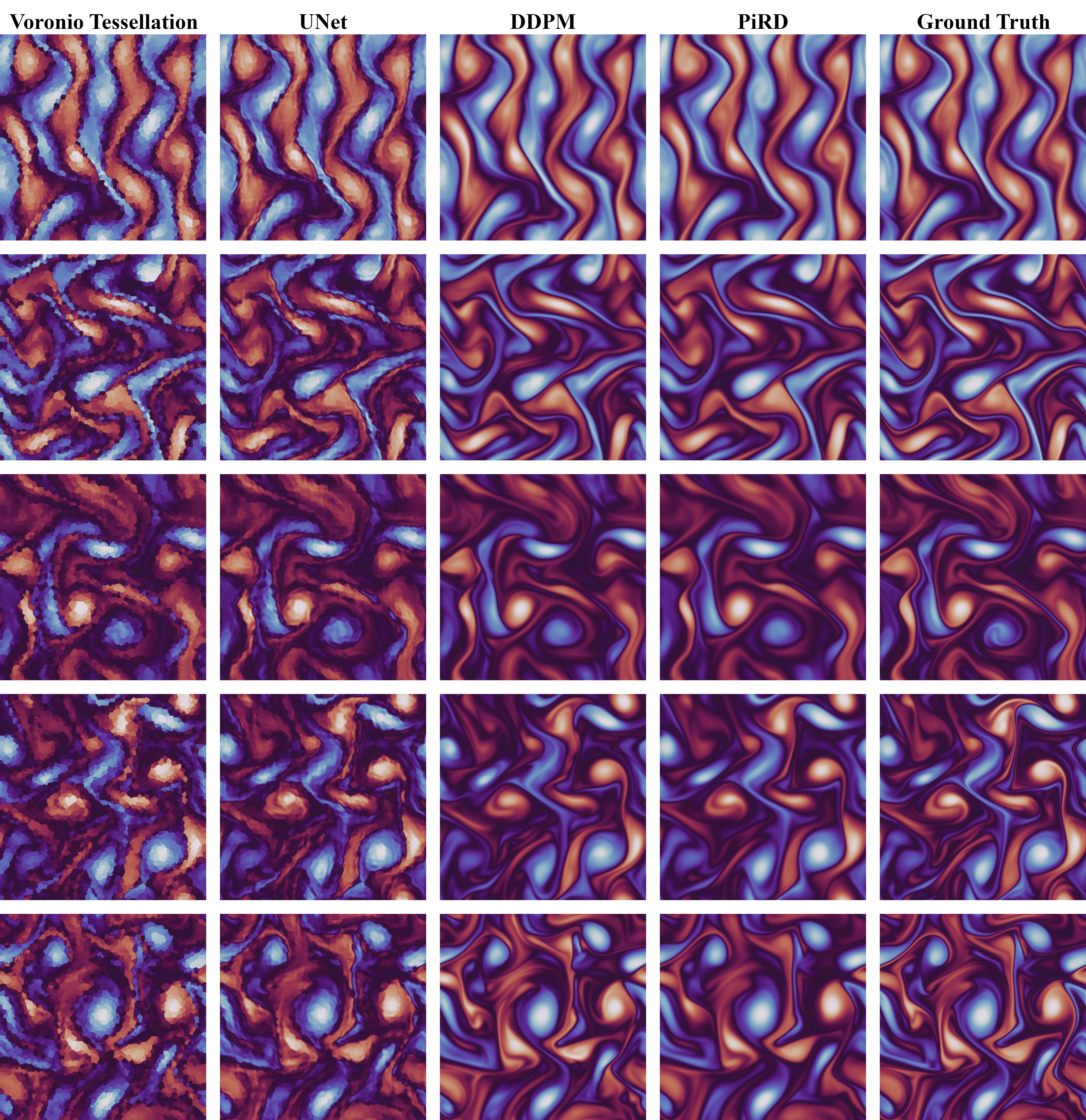
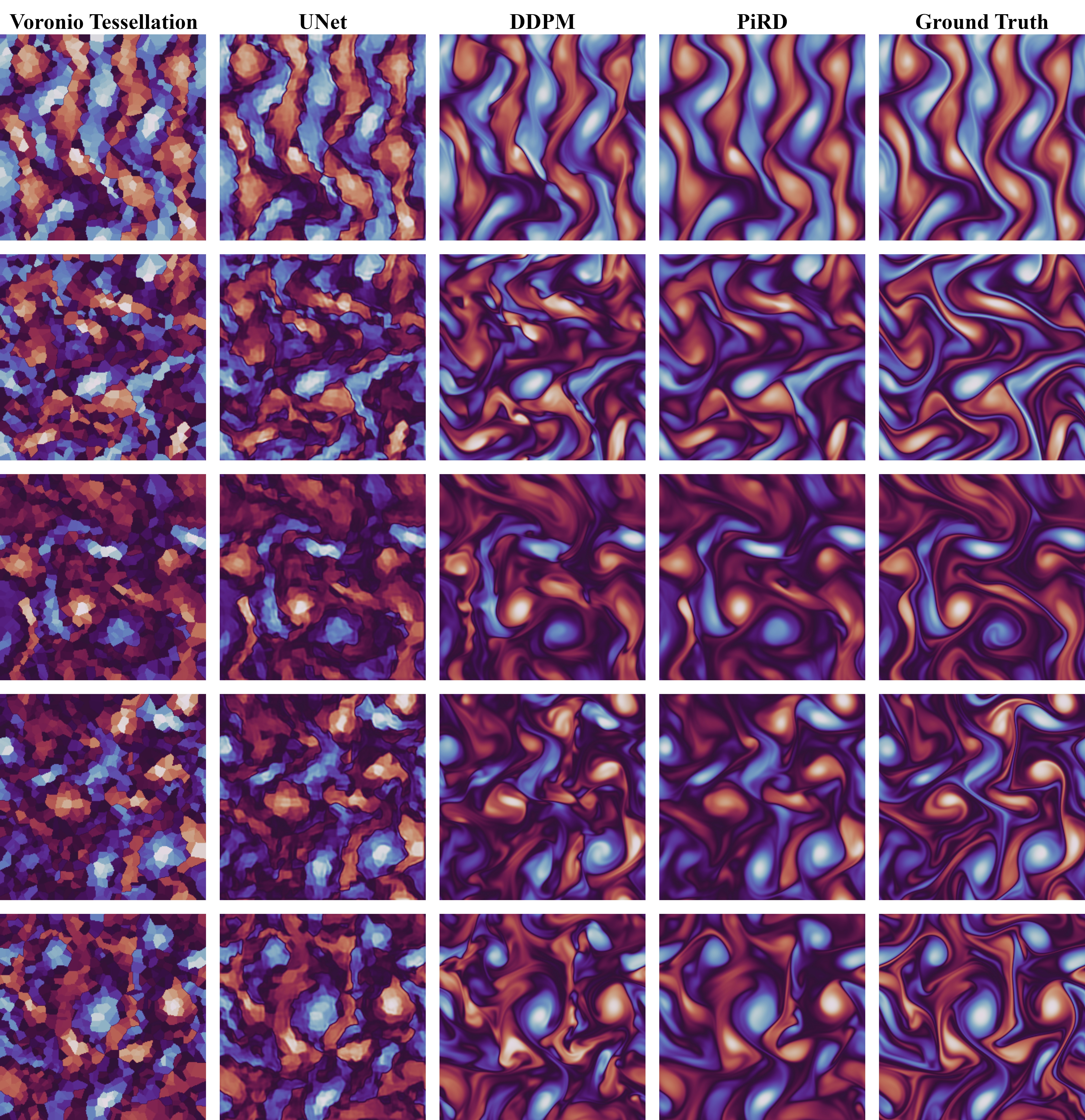
Subsequent tests evaluate the Mean Relative Error (MRE) and Partial Differential Equation (PDE) loss across four different tasks: up-sampling, up-sampling, , and reconstruction to resolution. For our training and testing, we first use bicubic interpolation on the up-sampling task and Voronoi tessellation on the reconstruction task to make the input matches the desired dimension of our output (), we then use nearest interpolation on the up-sampling tasks for testing the result, such that all the testing distributions and patterns are UNSEEN for PiRD, UNet, and Noisy Unet for fair comparison. We also iterate each batch 10 times and take the average of the flow fields as our final prediction. This approach is designed to reduce the influence of any randomness in the predictive outcomes. For training PiRD, steps for sampling in each iteration and was set to 2. In comparison, results for the physics-informed DDPM are generated using the hyper-parameters recommended by the original authors, with Discrete Denoising Implicit Models (DDIM) sampling steps set at 30 and 60 respectively.
| Methods | 4x | 8x | 5% | 1.5625% | ||||
| MRE | PDE | MRE | PDE | MRE | PDE | MRE | PDE | |
| PiRD(ours) | 0.1178 | 2.0663 | 0.3580 | 2.1594 | 0.2782 | 1.6939 | 0.3857 | 2.0917 |
| DDPM-based - 30 | 0.2832 | 8.0110 | 0.5251 | 7.4526 | 0.2811 | 3.7741 | 0.3912 | 14.7641 |
| DDPM-based - 60 | 0.2844 | 5.1598 | 0.5258 | 4.6567 | 0.2881 | 2.1297 | 0.4378 | 3.8925 |
| Noisy UNet | 0.2190 | 10.0515 | 0.4015 | 8.7777 | 0.3315 | 6.6934 | 0.4073 | 6.7641 |
| UNet | 0.1207 | 259.0664 | 0.3995 | 699.3475 | 0.3478 | 668.0065 | 0.4981 | 998.8791 |
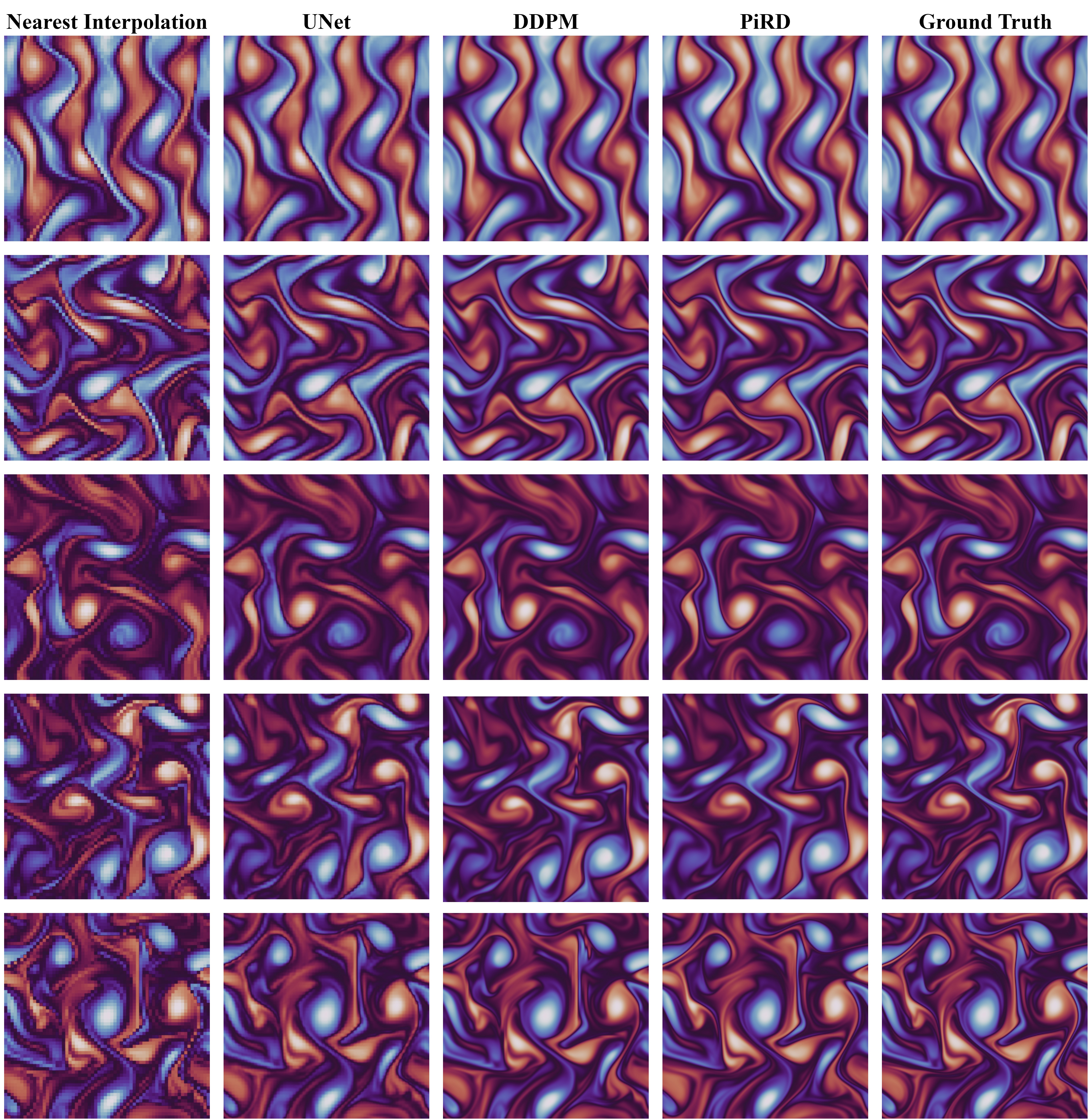
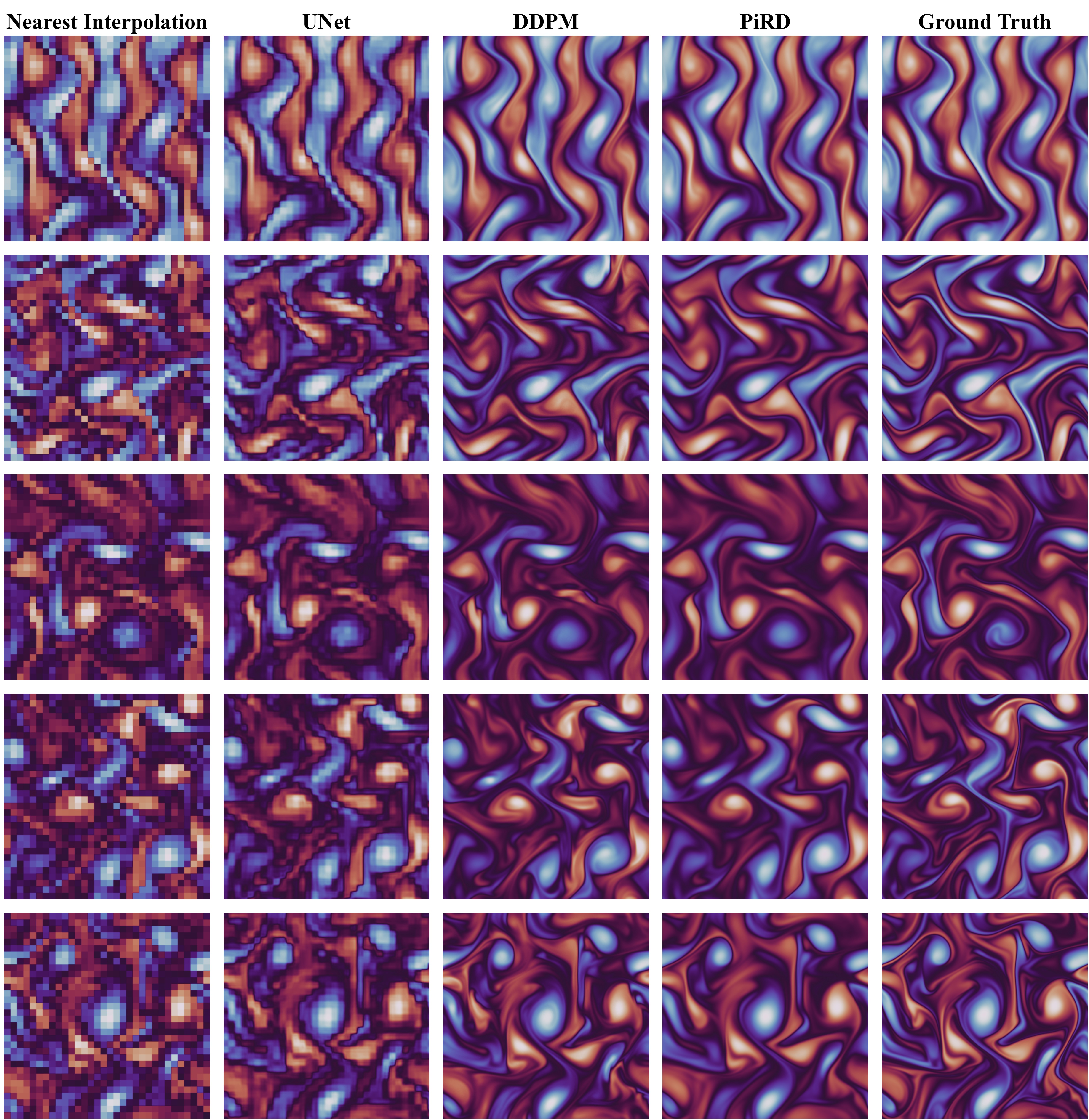
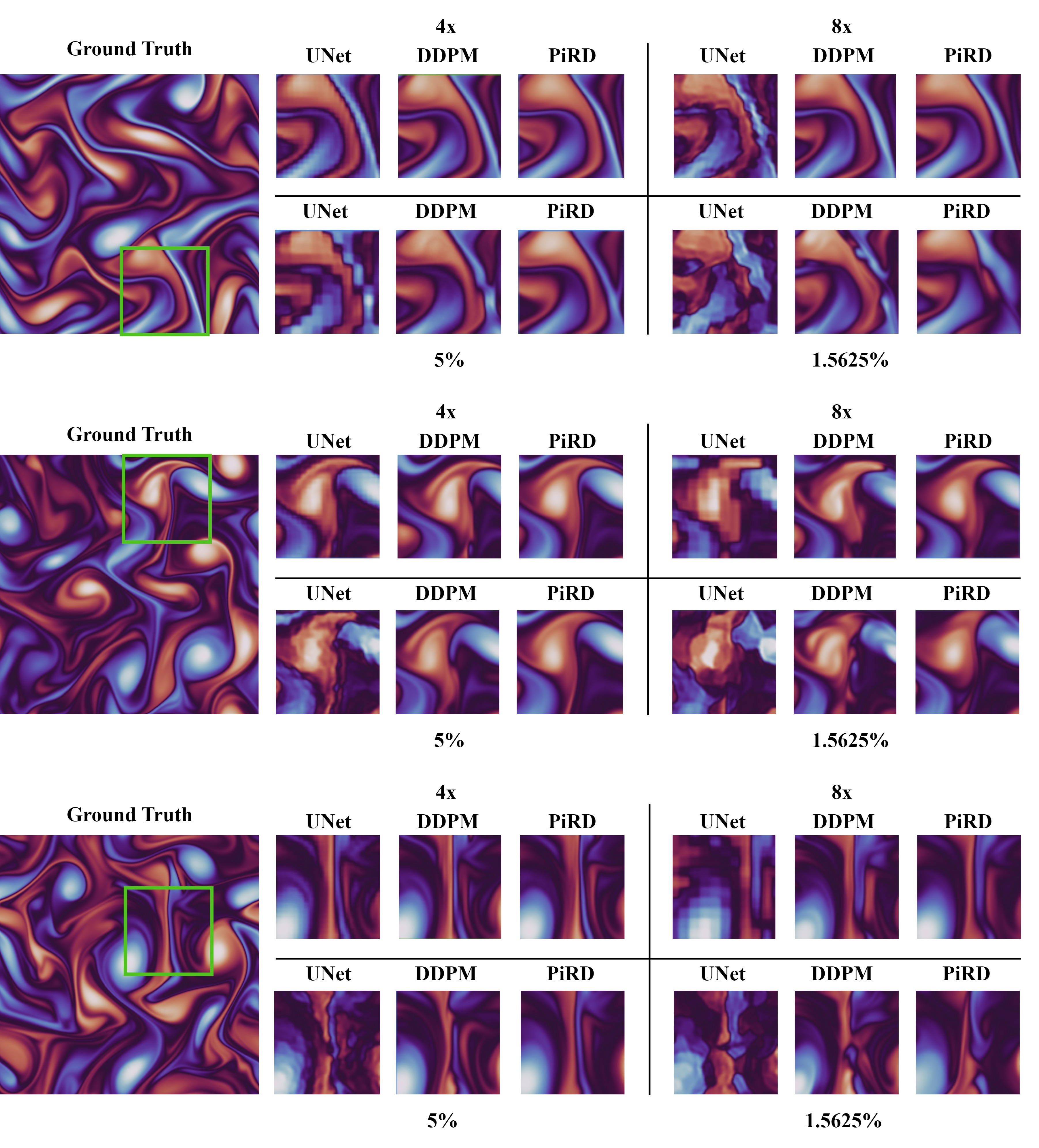
As illustrated in Table 1, UNet model struggles across all the tested scenarios particularly in terms of the PDE loss, reflecting its inability to generalize to unseen low-fidelity datasets encountered during training. Although it achieves the second lowest MRE on the 4x up-sampling task, it performs worst on recovering the underlying physical law. The extremely high PDE loss validates our opinion that the flow field reconstruction cannot be merely seen as a computer vision task, which may result in a successful recovery of element-wise information, but unacceptable physical-wise information. This can be further validated by visualizing the sampled flow fields in Figure 2. As shown, UNet model fails to generate reasonable or smooth flow fields, especially when the low-fidelity input contains randomly distributed measurements (e.g., the and reconstruction tasks).
Conversely, the PiRD, DDPM-based and Noisy UNet methods maintained low and reasonable PDE losses, indicating successful recovery of the underlying physical laws during the reconstruction process while containing a low mean relative error. Notably, PiRD performs best on all scenarios on both MRE and PDE loss, which validates our assumption that all different low-fidelity scenarios can first be mapped into a collective noisy LF distribution and then one can utilize the learned reverse Markov chain to sample the LF flow fields back to the HF distribution.
It is noteworthy that the DDPM-based method’s performance on PDE loss is dependent on the number of sampling steps employed; increasing the steps from 30 to 60 tends to reduce PDE loss but at the expense of higher MRE. This trade-off arises because the DDPM-based method involves subtracting the PDE deviation relative to the vorticity field at each sampling step — a process that is challenging to manage without potentially compromising MRE performance. In contrast, our PiRD model excels in predicting the high-fidelity field with both a remarkably low MRE and an exceptionally low PDE loss, showcasing its effectiveness and robustness in the flow field reconstruction task. For a comprehensive and varied examination of PiRD’s performance, we invite readers to consult the Appendix section, where the reconstructed flow fields with different inputs are presented.
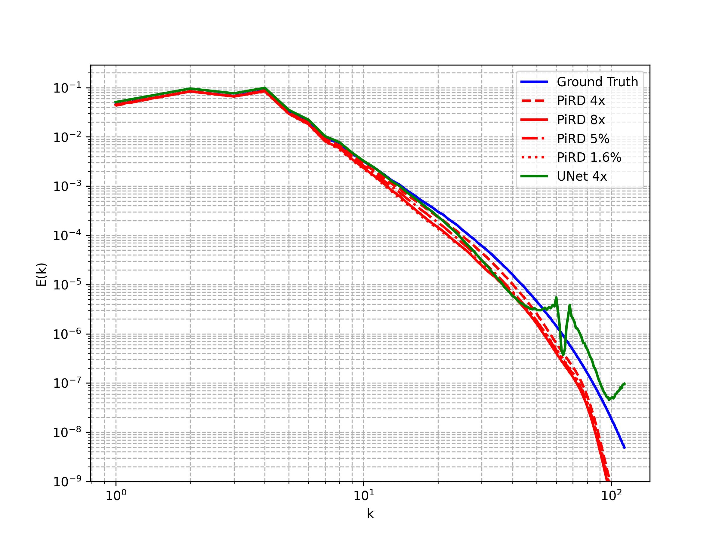
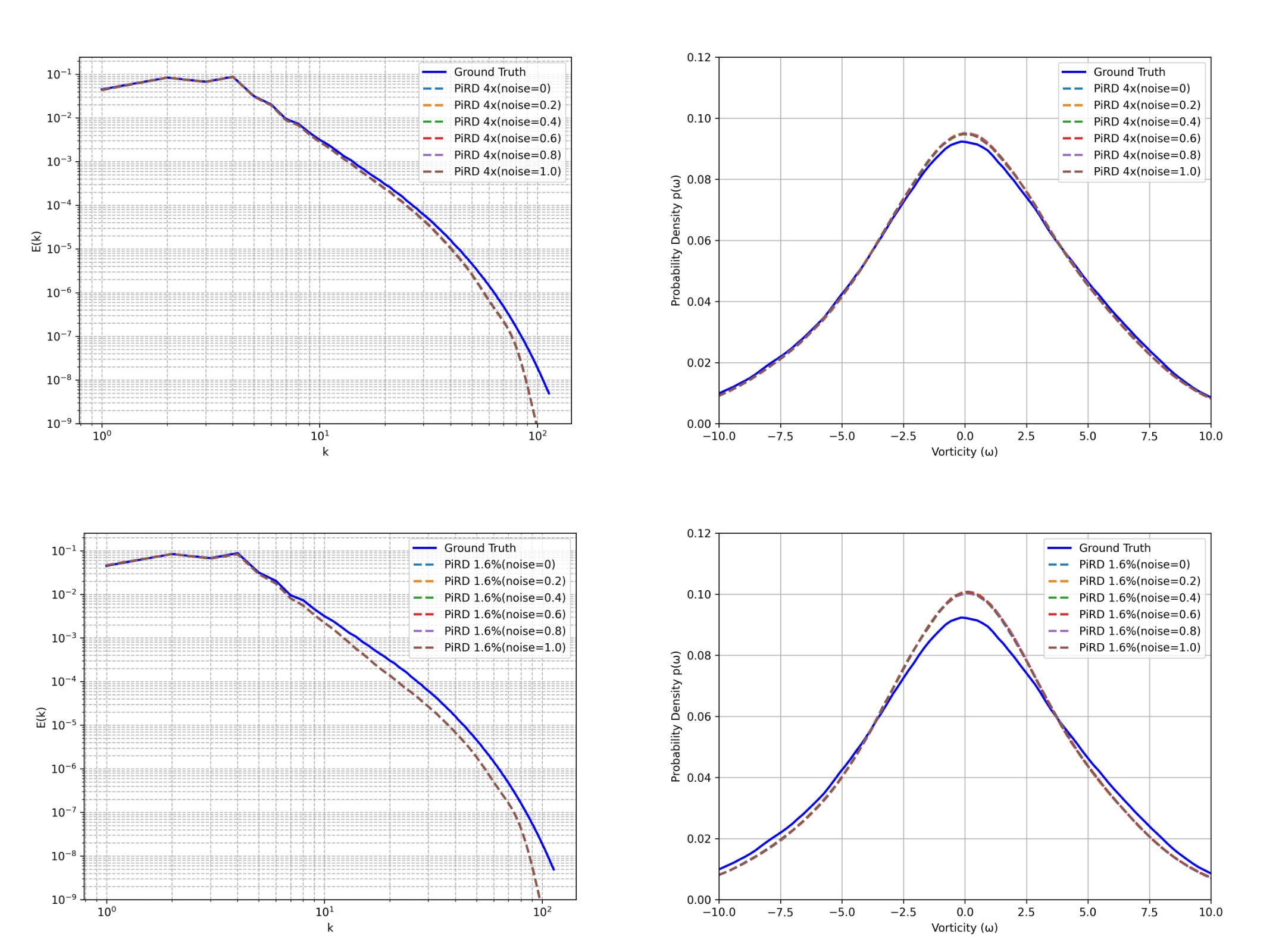
4.2 Evaluation on kinetic energy spectrum and vorticity distribution
The kinetic energy spectrum is a crucial metric in turbulence research and is used to understand the distribution of energy among different scales within the flow field. It characterizes how kinetic energy varies with the wavenumber, revealing the flow’s energy cascade from larger to smaller scales. It is important to highlight that despite UNet’s mean relative error (MRE) being comparable to that of PiRD for the task of 4x up-sampling, as indicated in Table 1, its performance on the kinetic energy spectrum is relatively poor, as shown in Figure 3(a). Although it performs well in recovering large-scale vortices, it fails to retrieve the vorticity at higher wavenumber. This discrepancy further validates our view that the accurate recovery of element-wise data does not necessarily translate to successfully retrieving physically meaningful information. On the contrary, our method demonstrates a robust capability to recover the energy distribution of the turbulent flow as shown in Figure 3(a). The spectrum obtained by our technique aligns closely with the ground truth across a range of wavenumbers, particularly in the inertial subrange, indicating that our method successfully captures the scale-dependent distribution of kinetic energy. The slight deviation at higher wavenumbers can be attributed to the inherent challenges in resolving the smallest scales of turbulence.
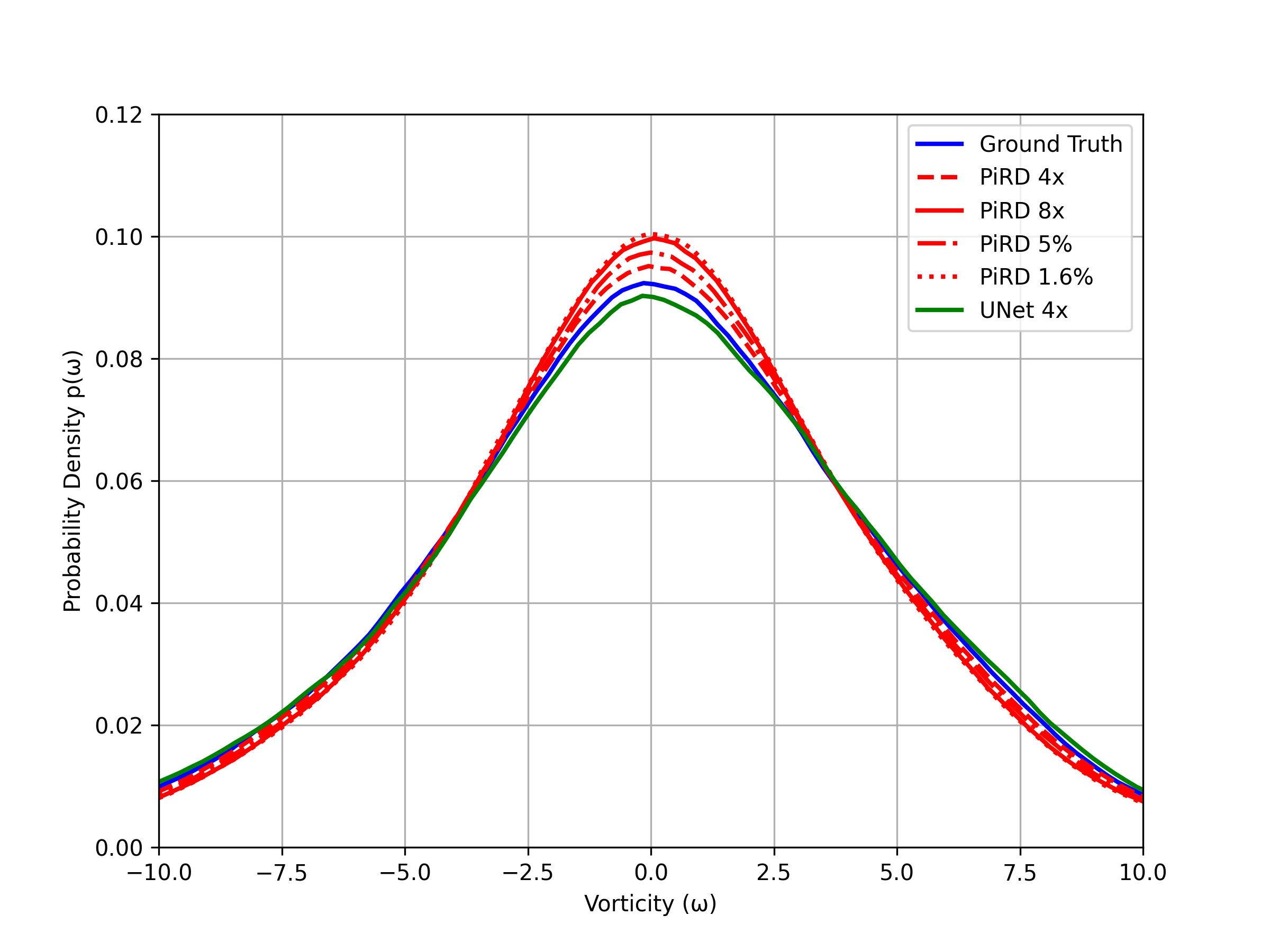
Moreover, the vorticity distribution provides insight into the probability of finding certain vorticity magnitudes within the flow. A method that accurately captures the vorticity distribution from coarse data suggests it can retain critical features of the turbulence structure, such as vortex stretching and tilting mechanisms. The vorticity distribution shown in Figure 3(b) further confirms the efficacy of our proposed approach. The recovered distribution exhibits a strong agreement with the ground truth, especially in capturing the peak and the tails of the distribution, which are indicative of the extreme vorticity events in the flow.
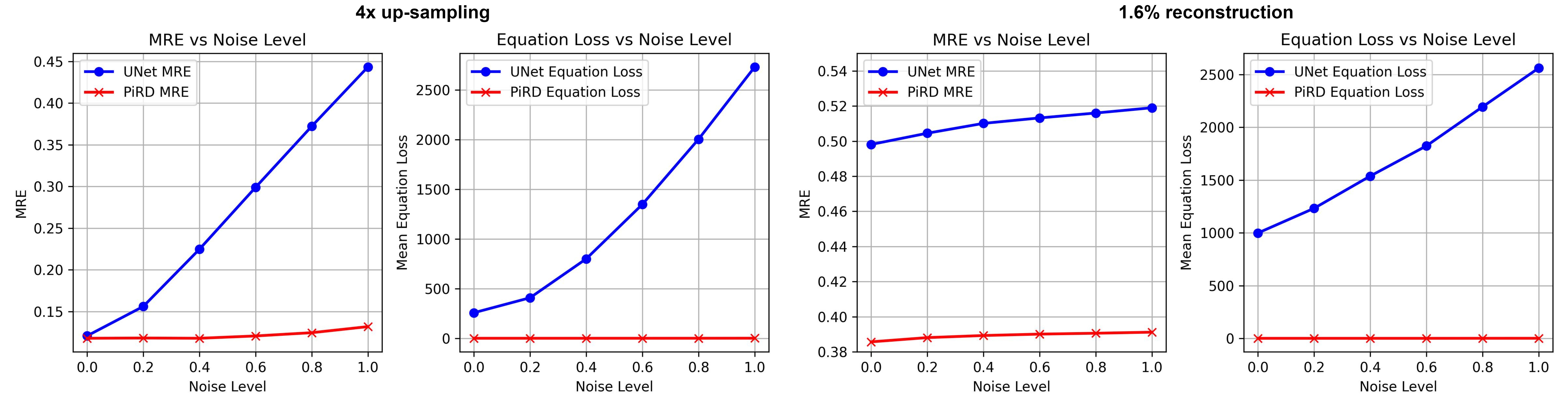
4.3 Evaluation on noisy low-fidelity vorticity field
In this section, we investigate the robustness of PiRD against a progressive density of Gaussian noise injected into the low-fidelity input, the noise injection and prediction process can be described below
| (21) |
where ranges from 0.2 to 1.0 by a step size of 0.2, the low-fidelity field is down-sampled from the high-fidelity one by a scale of 4, and randomly selected 1.5625% of the high-fidelity data respectively, and then normalized to Gaussian distribution before noise is injected. Table 2 illustrates the performance of MRE and PDE loss of PiRD and UNet under different noise levels for a 4x and a 1.5625% reconstruction task respectively. As shown in Figure 4, as the injected noise density increases, UNet’s performance degrades significantly. On the contrary, PiRD has stably and accurately predicted the HF field for both scenarios. In addition, as illustrated in Figure 5, the kinetic energy spectrum and vorticity distribution appear identical across all noise densities compared to the case where no noise is injected. This observation suggests that PiRD is highly robust to noise interference. Although there is a slight degradation in MRE as the noise density increases, the performance on PDE loss, vorticity distribution, and kinetic energy spectrum remains consistent.
| Noise Level | MRE | Equation Loss | ||||||
| 4x | 4x | |||||||
| UNet | PiRD | UNet | PiRD | UNet | PiRD | UNet | PiRD | |
| 0.0 | 0.1207 | 0.1178 | 0.4981 | 0.3857 | 259.0664 | 2.0663 | 998.8791 | 2.0917 |
| 0.2 | 0.1560 | 0.1181 | 0.5045 | 0.3881 | 409.8747 | 2.0563 | 1232.7024 | 2.0917 |
| 0.4 | 0.2247 | 0.1178 | 0.5101 | 0.3893 | 801.6868 | 2.1201 | 1537.9834 | 2.0837 |
| 0.6 | 0.2990 | 0.1206 | 0.5132 | 0.3901 | 1350.3967 | 2.1059 | 1823.7584 | 2.0946 |
| 0.8 | 0.3723 | 0.1245 | 0.5160 | 0.3903 | 2006.1515 | 2.3082 | 2093.8465 | 2.3822 |
| 1.0 | 0.4435 | 0.1318 | 0.5190 | 0.3912 | 2733.3027 | 2.7030 | 2560.6975 | 2.5433 |
5 Conclusion
This study highlights the inherent limitations of conventional CNN-based methods in reconstructing flow fields. Specifically, these methods tend to perform optimally only on data that mirrors the distribution or down-sampling processes they were originally trained on. A mere adaptation of computer vision techniques to flow field reconstruction tasks often leads to results that, while visually plausible, may not adhere strictly to the mathematical and physical principles governing the flow dynamics.
Our proposed model, PiRD, is expected to address these challenges by establishing a Markov chain that links low-fidelity and high-fidelity flow fields. This approach not only ensures the retention of physical laws throughout the training and sampling processes but also exhibits remarkable resilience to various down-sampling operations. By prioritizing both element-wise accuracy and adherence to physical laws, PiRD may set a new benchmark in performance across experimental datasets. PiRD is demonstrated to be promising for flow field reconstruction tasks, merging the realms of deep learning and fluid dynamics with unprecedented efficacy.
As the first attempt to apply the ResShift diffusion model for the flow field reconstruction problem, the proposed method still has some limitations. While PiRD demonstrates enhanced accuracy and robustness over CNN-based models when dealing with unseen sparse and noisy measurements, its performance can be further optimized when the training and testing sets are under the same distribution. In the near future, incorporating more controllable physical flow information into diffusion model training, as an alternative to the conventional stacking of Gaussian noises, may be a promising direction for developing a more accurate and generalizable flow generation model.
References
- [1] Kevin Course and Prasanth B Nair. State estimation of a physical system with unknown governing equations. Nature, 622(7982):261–267, 2023.
- [2] N Benjamin Erichson, Lionel Mathelin, Zhewei Yao, Steven L Brunton, Michael W Mahoney, and J Nathan Kutz. Shallow neural networks for fluid flow reconstruction with limited sensors. Proceedings of the Royal Society A, 476(2238):20200097, 2020.
- [3] Huanfeng Shen, Xinghua Li, Qing Cheng, Chao Zeng, Gang Yang, Huifang Li, and Liangpei Zhang. Missing information reconstruction of remote sensing data: A technical review. IEEE Geoscience and Remote Sensing Magazine, 3(3):61–85, 2015.
- [4] Saiprasad Ravishankar, Jong Chul Ye, and Jeffrey A Fessler. Image reconstruction: From sparsity to data-adaptive methods and machine learning. Proceedings of the IEEE, 108(1):86–109, 2019.
- [5] Steven L Brunton, Bernd R Noack, and Petros Koumoutsakos. Machine learning for fluid mechanics. Annual review of fluid mechanics, 52:477–508, 2020.
- [6] Keyi Wu, Peng Chen, and Omar Ghattas. A fast and scalable computational framework for large-scale high-dimensional bayesian optimal experimental design. SIAM/ASA Journal on Uncertainty Quantification, 11(1):235–261, 2023.
- [7] Ugo Piomelli. Large-eddy simulation: achievements and challenges. Progress in Aerospace Sciences, 35(4):335–362, 1999.
- [8] Giancarlo Alfonsi. Reynolds-averaged navier–stokes equations for turbulence modeling. 2009.
- [9] Stefan Heinz. A review of hybrid RANS-LES methods for turbulent flows: Concepts and applications. Progress in Aerospace Sciences, 114:100597, 2020.
- [10] Mengze Wang and Tamer A Zaki. State estimation in turbulent channel flow from limited observations. Journal of Fluid Mechanics, 917:A9, 2021.
- [11] Mengze Wang, Qi Wang, and Tamer A Zaki. Discrete adjoint of fractional-step incompressible Navier-Stokes solver in curvilinear coordinates and application to data assimilation. Journal of Computational Physics, 396:427–450, 2019.
- [12] Chao Dong, Chen Change Loy, Kaiming He, and Xiaoou Tang. Image super-resolution using deep convolutional networks. IEEE transactions on pattern analysis and machine intelligence, 38(2):295–307, 2015.
- [13] Chunwei Tian, Yong Xu, Wangmeng Zuo, Bob Zhang, Lunke Fei, and Chia-Wen Lin. Coarse-to-fine cnn for image super-resolution. IEEE Transactions on Multimedia, 23:1489–1502, 2020.
- [14] Xiangyu Chen, Xintao Wang, Jiantao Zhou, Yu Qiao, and Chao Dong. Activating more pixels in image super-resolution transformer. In Proceedings of the IEEE/CVF Conference on Computer Vision and Pattern Recognition, pages 22367–22377, 2023.
- [15] Fuzhi Yang, Huan Yang, Jianlong Fu, Hongtao Lu, and Baining Guo. Learning texture transformer network for image super-resolution. In Proceedings of the IEEE/CVF Conference on Computer Vision and Pattern Recognition, pages 5791–5800, 2020.
- [16] Ziwei Luo, Youwei Li, Shen Cheng, Lei Yu, Qi Wu, Zhihong Wen, Haoqiang Fan, Jian Sun, and Shuaicheng Liu. Bsrt: Improving burst super-resolution with swin transformer and flow-guided deformable alignment. In Proceedings of the IEEE/CVF Conference on Computer Vision and Pattern Recognition, pages 998–1008, 2022.
- [17] Chenyu You, Guang Li, Yi Zhang, Xiaoliu Zhang, Hongming Shan, Mengzhou Li, Shenghong Ju, Zhen Zhao, Zhuiyang Zhang, Wenxiang Cong, et al. Ct super-resolution GAN constrained by the identical, residual, and cycle learning ensemble (GAN-CIRCLE). IEEE Transactions on Medical Imaging, 39(1):188–203, 2019.
- [18] Sefi Bell-Kligler, Assaf Shocher, and Michal Irani. Blind super-resolution kernel estimation using an internal-GAN. Advances in Neural Information Processing Systems, 32, 2019.
- [19] Kui Jiang, Zhongyuan Wang, Peng Yi, Guangcheng Wang, Tao Lu, and Junjun Jiang. Edge-enhanced gan for remote sensing image superresolution. IEEE Transactions on Geoscience and Remote Sensing, 57(8):5799–5812, 2019.
- [20] Romit Maulik, Kai Fukami, Nesar Ramachandra, Koji Fukagata, and Kunihiko Taira. Probabilistic neural networks for fluid flow surrogate modeling and data recovery. Physical Review Fluids, 5(10):104401, 2020.
- [21] Han Gao, Luning Sun, and Jian-Xun Wang. Super-resolution and denoising of fluid flow using physics-informed convolutional neural networks without high-resolution labels. Physics of Fluids, 33(7), 2021.
- [22] Luning Sun and Jian-Xun Wang. Physics-constrained bayesian neural network for fluid flow reconstruction with sparse and noisy data. Theoretical and Applied Mechanics Letters, 10(3):161–169, 2020.
- [23] Amirhossein Arzani, Jian-Xun Wang, and Roshan M D’Souza. Uncovering near-wall blood flow from sparse data with physics-informed neural networks. Physics of Fluids, 33(7), 2021.
- [24] Tomoki Asaka, Katsunori Yoshimatsu, and Kai Schneider. Machine learning-based vorticity evolution and super-resolution of homogeneous isotropic turbulence using wavelet projection. Physics of Fluids, 36(2), 2024.
- [25] Roger Ratcliff, Philip L Smith, Scott D Brown, and Gail McKoon. Diffusion decision model: Current issues and history. Trends in cognitive sciences, 20(4):260–281, 2016.
- [26] Diederik Kingma, Tim Salimans, Ben Poole, and Jonathan Ho. Variational diffusion models. Advances in Neural Information Processing Systems, 34:21696–21707, 2021.
- [27] Jonathan Ho, Ajay Jain, and Pieter Abbeel. Denoising diffusion probabilistic models. Advances in Neural Information Processing Systems, 33:6840–6851, 2020.
- [28] Dule Shu, Zijie Li, and Amir Barati Farimani. A physics-informed diffusion model for high-fidelity flow field reconstruction. Journal of Computational Physics, 478:111972, 2023.
- [29] Zongsheng Yue, Jianyi Wang, and Chen Change Loy. Resshift: Efficient diffusion model for image super-resolution by residual shifting. Advances in Neural Information Processing Systems, 36, 2024.
- [30] Pranshu Pant and Amir Barati Farimani. Deep learning for efficient reconstruction of high-resolution turbulent dns data. arXiv preprint arXiv:2010.11348, 2020.
Appendix